anomaly detection in predictive maintenance - knime · anomaly detection in predictive maintenance...

Copyright © 2014 by KNIME.com AG all rights reserved page 1

Anomaly Detection in Predictive

Maintenance Anomaly Detection with Time Series Analysis

Phil Winters [email protected] Iris Adae [email protected] Rosaria Silipo [email protected]

mailto:[email protected]




Table of Contents Anomaly Detection in Predictive Maintenance Anomaly Detection with Time Series Analysis .................................................................................................................................................. 1

Summary ................................................................................................................................................. 3

Anomaly Detection as a Time Series Problem ........................................................................................ 3

Data and Pre-Processing ......................................................................................................................... 4

Anomaly Detection Based on Chart Control ........................................................................................... 5

Boundaries Calculation for “Normal” Values ...................................................................................... 5

Level 1 Alarm ....................................................................................................................................... 6

Level 2 Alarm ....................................................................................................................................... 6

Taking Action ....................................................................................................................................... 7

Anomaly Detection Based on Auto-Regressive Models .......................................................................... 8

Training: Learning the “normal” signal with an AR model .................................................................. 8

Deployment: Level 1 Alarm ................................................................................................................. 9

Deployment: Level 2 Alarm ............................................................................................................... 10

Deployment: Taking Action ............................................................................................................... 11

Conclusions ............................................................................................................................................ 12


Summary This whitepaper is the second of the series on anomaly detection for predictive maintenance (https://www.knime.org/white-papers under IoT/Anomaly Detection). The first whitepaper explained the basic work to prepare data, including data cleaning, data preparation and aggregation, and data visualization.

This whitepaper deals with the recognition of early signs of anomalies in the sensor signals monitoring a working rotor. We inherited the processed data set from the first whitepaper (IoT/Anomaly Detection I: Time Alignment and Visualization for Anomaly Detection), as 393 time series for different frequency bands and different sensor locations on the rotor. Our current goal is to be able to predict a breakdown episode without any previous examples.

We separate the time line into a training window, with the rotor working properly; a maintenance window, where we look for early anomaly signs before the breakdown episode; and a final window, where the rotor has been repaired and works again properly.

Signals in the training window describe a normally working rotor. We use this “normality” data to train a model for time series prediction. Given the nature of the training data, therefore, this model will only be able to predict sample values for a properly working rotor.

In the next time window, the maintenance window, we look for signs of disruption from this “normality” situation. If the model predictions start getting more and more distant from reality, this could be an alarming sign that the underlying system has changed. In this case a series of mechanical checkups must be triggered.

Here we investigate two techniques for anomaly detection using time series prediction: control chart and auto-regressive models. Workflows and data used for this whitepaper can be found on the KNIME EXAMPLES server under 050_Applications/050017_AnomalyDetection/Time Series Analysis.

Anomaly Detection as a Time Series Problem We are all witnessing the current explosion of data: social media data, clinical data, system data, CRM data, web data, and lately tons of sensor data! With the advent of the Internet of Things, systems and monitoring applications are producing humongous amounts of data which undergo evaluation to optimize costs and benefits, predict future events, classify behaviors, implement quality control, and more. All these use cases have been relatively well established by now: a goal is defined, a target class is selected, a model is trained to recognize/predict a target, and the same model is applied to new never-seen-before productive data.

The newest challenge now lies in predicting the “unknown”. The “unknown” is an event that is not part of the system past, an event that cannot be found in the system’s historical data. In the case of network data the “unknown” event can be an intrusion, in medicine a sudden pathological status, in sales or credit card businesses a fraudulent payment, and, finally, in machinery a mechanical piece breakdown. A high value, in terms of money, life expectancy, and/or time, is usually associated with the early discovery, warning, prediction, and/or prevention of the “unknown” and, most likely, undesirable event.

Specifically, prediction of “unknown” disruptive events in the field of mechanical maintenance takes the name of “anomaly detection”.

Moving away from supervised anomaly detection, where one class is just labeled as anomaly, but examples of that class exist in historical data, we concentrate here on dynamic unsupervised anomaly detection (see first whitepaper of this series: IoT/Anomaly Detection I: Time Alignment and Visualization for Anomaly Detection).

https://www.knime.org/white-papers






In dynamic unsupervised anomaly detection, the word “dynamic” means that we approach the problem from a time perspective. Attributes and their evolutions are observed over time before the catastrophic previously unseen event occurs. The word “unsupervised” means that we are trying to predict an event that has no examples in the data history. So, the strategy involves monitoring the attribute evolutions over time in the anomaly-free historical data. Indeed deviations from the historical attribute evolutions can be warning signs of a future anomaly; these warning signs can then be used to trigger a generic anomaly alarm, requiring further checkups.

For example, when a motor is slowly deteriorating, one of the measurements might change gradually until eventually the motor breaks. On the one hand we want to keep the motor running as long as possible – mechanical pieces are expensive! ‒ on the other, we want to avoid the motor breaking down completely, producing even more damage.

As we described already in the first whitepaper on pre-processing and visualization for anomaly detection (IoT/Anomaly Detection I: Time Alignment and Visualization for Anomaly Detection), there is a lot of data that lends itself to unsupervised anomaly detection use cases: turbines, rotors, chemical reactions, medical signals, spectroscopy, and so on. In this whitepaper series we deal with rotor data.

We investigated two techniques for dynamic unsupervised anomaly detection.

The first technique, named Chart Control, defines boundaries for an anomaly-free functioning rotor. The boundaries are usually centered on the average signal value and bounded by twice the standard deviation in both directions. If the signal is wandering off this anomaly free area, an alarm should occur.

The second approach, based on an Auto-Regressive (AR) model, is conceptually similar to the Control Chart, but more sophisticated in its implementation. An anomaly-free time window is defined and this time window is used to train an auto-regressive model. The boundaries for anomaly-free functioning are defined here on the prediction errors on the training set. During deployment on new data, if the prediction error wanders off such boundaries, an alarm is fired off requiring further checkups.

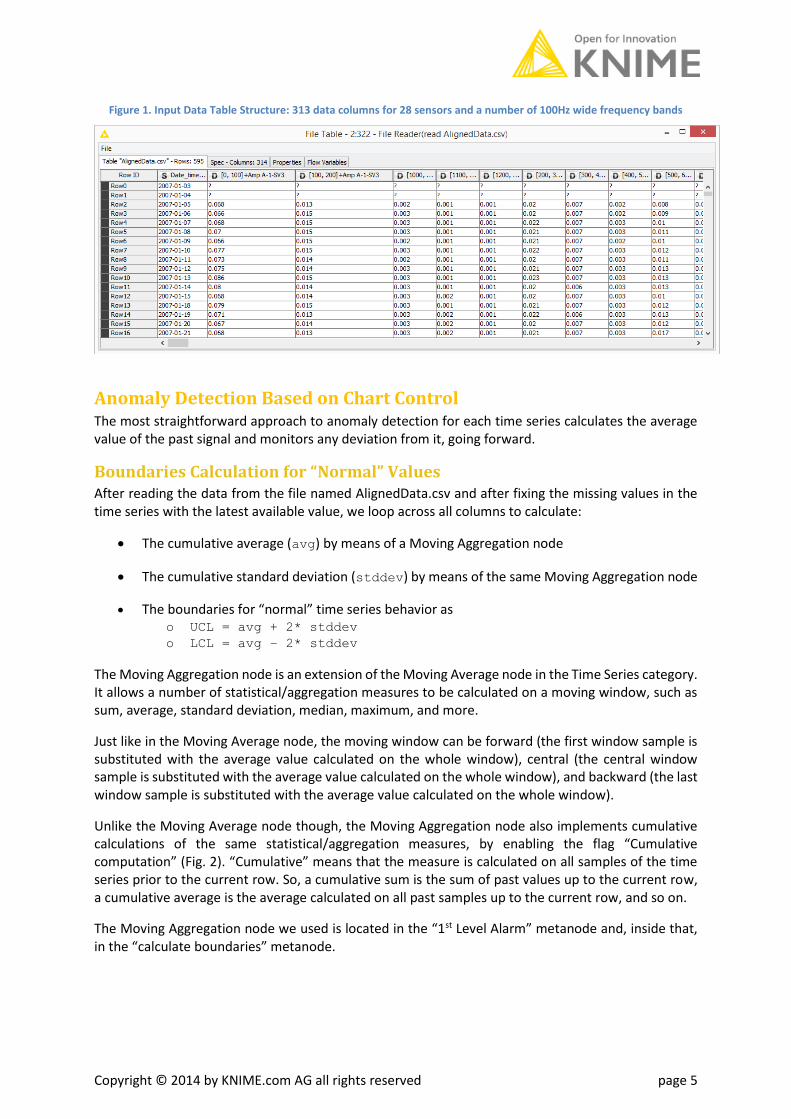
Data and Pre-Processing For a description of the original data, as time series of Fast Fourier Transform (FFT) spectral amplitudes and frequencies, we refer to the first whitepaper of the series (IoT/Anomaly Detection I: Time Alignment and Visualization for Anomaly Detection). Starting with 28 signals from 28 sensors, monitoring 8 different parts of the rotor, after FFT and aggregation into frequency bins and dates, we ended up with the data table in file AlignedData.csv.

This data table includes 313 spectral amplitude data columns and a date-time data column. Each spectral amplitude originates from one of the original 28 sensors and refers to one 100Hz-wide frequency band falling between 0Hz and 1200Hz.





Figure 1. Input Data Table Structure: 313 data columns for 28 sensors and a number of 100Hz wide frequency bands

Anomaly Detection Based on Chart Control The most straightforward approach to anomaly detection for each time series calculates the average value of the past signal and monitors any deviation from it, going forward.

Boundaries Calculation for “Normal” Values After reading the data from the file named AlignedData.csv and after fixing the missing values in the time series with the latest available value, we loop across all columns to calculate:

The cumulative average (avg) by means of a Moving Aggregation node

The cumulative standard deviation (stddev) by means of the same Moving Aggregation node

The boundaries for “normal” time series behavior as o UCL = avg + 2* stddev o LCL = avg – 2* stddev

The Moving Aggregation node is an extension of the Moving Average node in the Time Series category. It allows a number of statistical/aggregation measures to be calculated on a moving window, such as sum, average, standard deviation, median, maximum, and more.

Just like in the Moving Average node, the moving window can be forward (the first window sample is substituted with the average value calculated on the whole window), central (the central window sample is substituted with the average value calculated on the whole window), and backward (the last window sample is substituted with the average value calculated on the whole window).

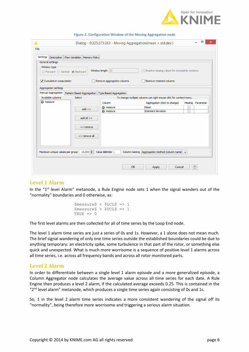
Unlike the Moving Average node though, the Moving Aggregation node also implements cumulative calculations of the same statistical/aggregation measures, by enabling the flag “Cumulative computation” (Fig. 2). “Cumulative” means that the measure is calculated on all samples of the time series prior to the current row. So, a cumulative sum is the sum of past values up to the current row, a cumulative average is the average calculated on all past samples up to the current row, and so on.

The Moving Aggregation node we used is located in the “1st Level Alarm” metanode and, inside that, in the “calculate boundaries” metanode.


Figure 2. Configuration Window of the Moving Aggregation node

Level 1 Alarm In the “1st level Alarm” metanode, a Rule Engine node sets 1 when the signal wanders out of the “normality” boundaries and 0 otherwise, as:

$messure$ < $LCL$ => 1

$messure$ > $UCL$ => 1

TRUE => 0

The first level alarms are then collected for all of time series by the Loop End node.

The level 1 alarm time series are just a series of 0s and 1s. However, a 1 alone does not mean much. The brief signal wandering of only one time series outside the established boundaries could be due to anything temporary: an electricity spike, some turbulence in that part of the rotor, or something else quick and unexpected. What is much more worrisome is a sequence of positive level 1 alarms across all time series, i.e. across all frequency bands and across all rotor monitored parts.

Level 2 Alarm In order to differentiate between a single level 1 alarm episode and a more generalized episode, a Column Aggregator node calculates the average value across all time series for each date. A Rule Engine then produces a level 2 alarm, if the calculated average exceeds 0.25. This is contained in the “2nd level alarm” metanode, which produces a single time series again consisting of 0s and 1s.

So, 1 in the level 2 alarm time series indicates a more consistent wandering of the signal off its “normality”, being therefore more worrisome and triggering a serious alarm situation.


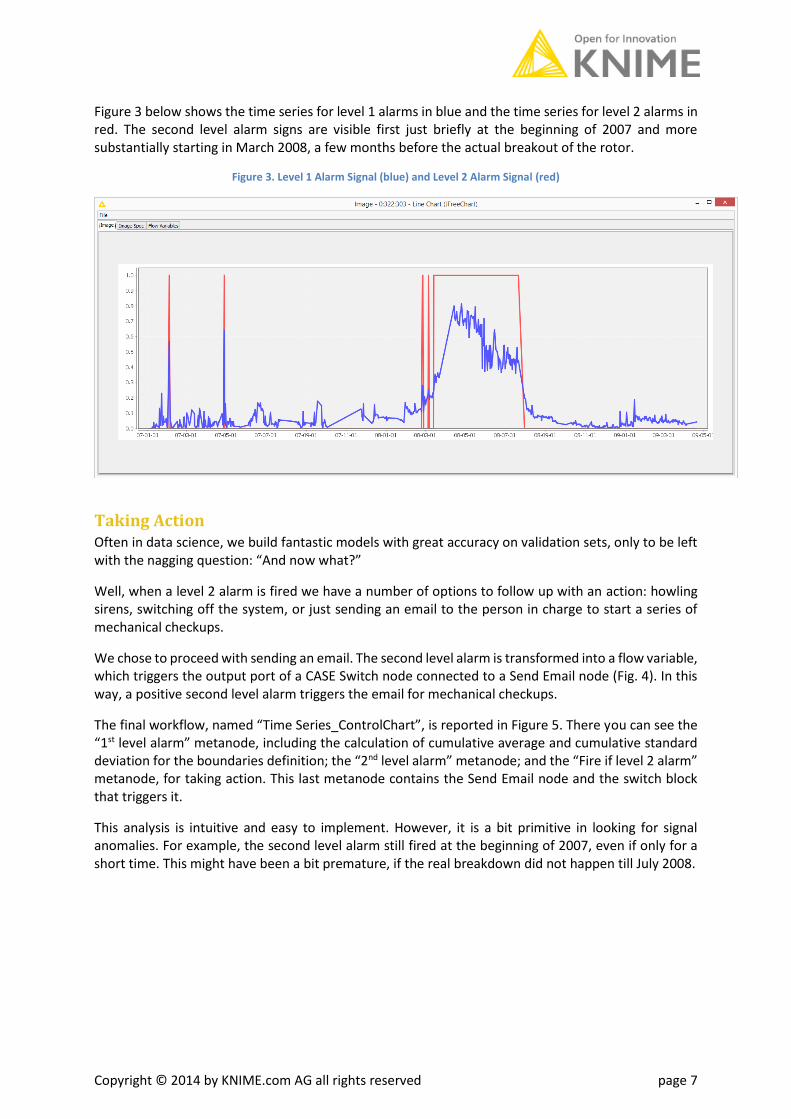
Figure 3 below shows the time series for level 1 alarms in blue and the time series for level 2 alarms in red. The second level alarm signs are visible first just briefly at the beginning of 2007 and more substantially starting in March 2008, a few months before the actual breakout of the rotor.

Figure 3. Level 1 Alarm Signal (blue) and Level 2 Alarm Signal (red)

Taking Action Often in data science, we build fantastic models with great accuracy on validation sets, only to be left with the nagging question: “And now what?”

Well, when a level 2 alarm is fired we have a number of options to follow up with an action: howling sirens, switching off the system, or just sending an email to the person in charge to start a series of mechanical checkups.

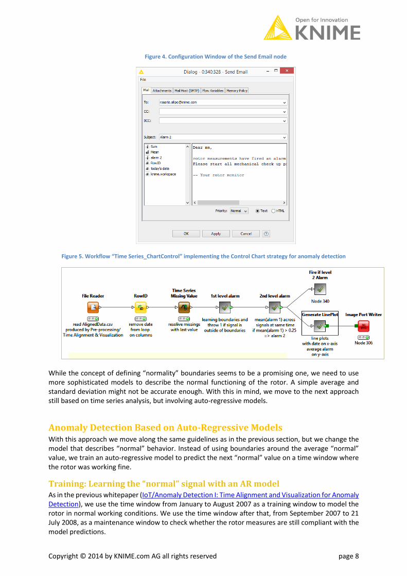
We chose to proceed with sending an email. The second level alarm is transformed into a flow variable, which triggers the output port of a CASE Switch node connected to a Send Email node (Fig. 4). In this way, a positive second level alarm triggers the email for mechanical checkups.

The final workflow, named “Time Series_ControlChart”, is reported in Figure 5. There you can see the “1st level alarm” metanode, including the calculation of cumulative average and cumulative standard deviation for the boundaries definition; the “2nd level alarm” metanode; and the “Fire if level 2 alarm” metanode, for taking action. This last metanode contains the Send Email node and the switch block that triggers it.

This analysis is intuitive and easy to implement. However, it is a bit primitive in looking for signal anomalies. For example, the second level alarm still fired at the beginning of 2007, even if only for a short time. This might have been a bit premature, if the real breakdown did not happen till July 2008.


Figure 4. Configuration Window of the Send Email node

Figure 5. Workflow “Time Series_ChartControl” implementing the Control Chart strategy for anomaly detection

While the concept of defining “normality” boundaries seems to be a promising one, we need to use more sophisticated models to describe the normal functioning of the rotor. A simple average and standard deviation might not be accurate enough. With this in mind, we move to the next approach still based on time series analysis, but involving auto-regressive models.

Anomaly Detection Based on Auto-Regressive Models With this approach we move along the same guidelines as in the previous section, but we change the model that describes “normal” behavior. Instead of using boundaries around the average “normal” value, we train an auto-regressive model to predict the next “normal” value on a time window where the rotor was working fine.

Training: Learning the “normal” signal with an AR model As in the previous whitepaper (IoT/Anomaly Detection I: Time Alignment and Visualization for Anomaly Detection), we use the time window from January to August 2007 as a training window to model the rotor in normal working conditions. We use the time window after that, from September 2007 to 21 July 2008, as a maintenance window to check whether the rotor measures are still compliant with the model predictions.




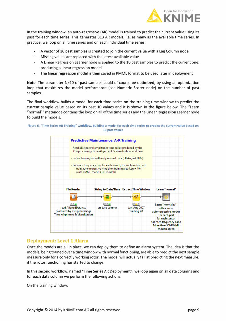
In the training window, an auto-regressive (AR) model is trained to predict the current value using its past for each time series. This generates 313 AR models, i.e. as many as the available time series. In practice, we loop on all time series and on each individual time series:

- A vector of 10 past samples is created to join the current value with a Lag Column node

- Missing values are replaced with the latest available value

- A Linear Regression Learner node is applied to the 10 past samples to predict the current one,

producing a linear regression model

- The linear regression model is then saved in PMML format to be used later in deployment

Note. The parameter N=10 of past samples could of course be optimized, by using an optimization loop that maximizes the model performance (see Numeric Scorer node) on the number of past samples.

The final workflow builds a model for each time series on the training time window to predict the current sample value based on its past 10 values and it is shown in the figure below. The “Learn “normal”“ metanode contains the loop on all of the time series and the Linear Regression Learner node to build the models.

Figure 6. “Time Series AR Training” workflow, building a model for each time series to predict the current value based on 10 past values

Deployment: Level 1 Alarm Once the models are all in place, we can deploy them to define an alarm system. The idea is that the models, being trained over a time window with normal functioning, are able to predict the next sample measure only for a correctly working rotor. The model will actually fail at predicting the next measure, if the rotor functioning has started to change.

In this second workflow, named “Time Series AR Deployment”, we loop again on all data columns and for each data column we perform the following actions.

On the training window:


- We apply the corresponding model to predict the current time series value based on its 10

past values

- We calculate the distance error between the original time series current value and the

predicted one

- We define: boundary = average(error) + 10*standard deviation(error)

On the maintenance window:

- We apply the corresponding model and we predict the current time series value based on the

10 past values

- We re-calculate the distance error between the original time series current value and the

predicted one

- We compare this distance error with the boundary defined on the training window as:

IF (distance *distance) > boundary THEN level 1 alarm = distance

Deployment: Level 2 Alarm Even here, a spike in the level 1 alarm time series does not really mean much. It could be due to an energy spike or turbulence in the rotor functioning. Thus, in order to make the alarm system more reliable, we use an aggregation of the level 1 alarm, like we did in the previous section. Here though, the aggregation is performed along the time dimension and not along the frequency dimension of the data set. With a Moving Aggregation node, the moving average of the level 1 alarm signal is calculated on a backward window of 21 samples. The backward window based moving average substitutes the last sample of the window with the average value of the previous samples in the same window. The backward window approach is necessary to simulate real life monitoring conditions, where past and current measures are available, but future measures are not.

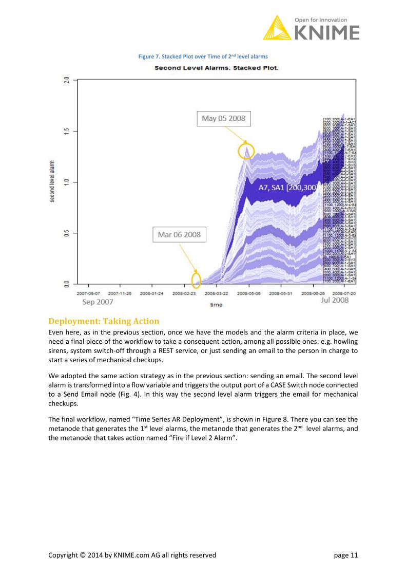
The moving average operation smooths out all random peaks in the level 1 alarm time series, and produces peaks in the 2nd level alarm time series, only if the level 1 alarm peaks persist over time. Figure 7 shows a stacked plot of the level 2 alarm time series obtained with an R View node over the maintenance time window. Here you can see that the early signs of the rotor malfunctioning can be tracked back as early as the beginning of March 2008. The definition of a sensitive threshold would allow the detection of these early malfunctioning episodes.

One might object that the optimization of a sensitive threshold is always a very difficult task and this is definitely true. However, even with a much less sensitive and far from perfect threshold, the stronger anomaly episodes starting on May 5, 2008 cannot be missed.

An optimization loop, maximizing the alarm performance, can help to define the optimal threshold on the 2nd level alarm values in terms of early anomaly detection.


Figure 7. Stacked Plot over Time of 2nd level alarms

Deployment: Taking Action Even here, as in the previous section, once we have the models and the alarm criteria in place, we need a final piece of the workflow to take a consequent action, among all possible ones: e.g. howling sirens, system switch-off through a REST service, or just sending an email to the person in charge to start a series of mechanical checkups.

We adopted the same action strategy as in the previous section: sending an email. The second level alarm is transformed into a flow variable and triggers the output port of a CASE Switch node connected to a Send Email node (Fig. 4). In this way the second level alarm triggers the email for mechanical checkups.

The final workflow, named “Time Series AR Deployment”, is shown in Figure 8. There you can see the metanode that generates the 1st level alarms, the metanode that generates the 2nd level alarms, and the metanode that takes action named “Fire if Level 2 Alarm”.


Figure 8. “Time Series AR Deployment” workflow, applying models and generating level 1 and level 2 alarms

Conclusions In this whitepaper we investigated two techniques based on time series prediction, in order to discover early signs of anomalies in a working rotor: control chart and auto-regressive models.

The idea was to train a model on signals from a normally working rotor, because that is all we have available, and then to compare the model predictions with the evolving signal to find possible early signs of system changes. Indeed, if the model predictions start getting more and more distant from reality, this could be an alarming sign that the underlying system has changed. In this case an email is triggered, setting in motion a series of mechanical checkups.

Workflows and data used for this whitepaper can be found on the KNIME EXAMPLES server under 050_Applications/050017_AnomalyDetection/Time Series Analysis

anomaly detection in predictive maintenance - knime · anomaly detection in predictive maintenance...

Documents