spatial statistics applied to commercial real estate statistics applied to commercial real estate...

J Real Estate Finan Econ (2010) 41:103–125DOI 10.1007/s11146-009-9190-2

Spatial Statistics Applied to Commercial Real Estate

Darren K. Hayunga · R. Kelley Pace

Published online: 21 May 2009© Springer Science + Business Media, LLC 2009

Abstract Portfolio theory shows that diversification can enhance the risk-return trade-off. This study uses the absolute location of commercial realestate property along with spatial statistics to address the inherent problemof determining geographical diversification based upon a set of economic andproperty-specific attributes, some of which are unobservable or must beproxied with noise. We find that commercial real estate portfolios exhibitstatistically significant spatial correlation at distances ranging from adjacentzip codes to neighboring metropolitan areas. Given the common structure

Research supported by a grant from the Real Estate Research Institute. We thankan anonymous referee, Richard Buttimer, the editor, Jeff Fisher, David Geltner,Marc Louargand, Glenn Mueller, Tony Sanders, C.F. Sirmans, and seminar participantsat the RERI conference, UNC-Charlotte, and UT-Arlington for their suggestions andguidance. Special thanks to Robert White of Real Capital Analytics for data.

D. K. Hayunga (B)Department of Finance and Real Estate,University of Texas at Arlington, Box 19449,Arlington, TX 76019, USAe-mail: [email protected]

R. K. PaceLREC Endowed Chair of Real Estate, Department of Finance,E.J. Ourso College of Business Administration,Louisiana State University, Baton Rouge, LA 70803-6308, USAe-mail: [email protected]: www.spatial-statistics.com

104 D.K. Hayunga, R.K. Pace

of dependence found in the data series, we discuss feasible strategies forobtaining diversification within direct-investment real estate portfolios.

Keywords Spatial statistics · Commercial real estate · Portfolio diversification

With the introduction of inefficiencies into the real estate market such as thosesuggested by Roulac (1976), diversification of portfolios that directly invest inreal estate assets is more complex than stock and bond portfolios. Specifically,the local or spatial nature of real estate markets introduces a trade-off betweenspecialization and spatial diversification.

On the one hand, specialization enables investors to continue learningand trading in previously researched and traded assets. To the extent suchinformation is costly, investors may be able to obtain a more precise under-standing of future payoffs at a lower price.1 In applying specialization to adirect-investment real estate portfolio, a manager may reduce information andmanagement costs as well as potentially increase returns from greater local-market information.

On the other hand, specialization in managing real estate portfolios impliesholding properties within a limited geographic area (e.g., neighborhood ormetropolitan area). Since neighboring properties experience similar supplyand demand functions, labor markets, and regulations, prices of these proper-ties within close proximity of each other will be positively correlated. However,traditional diversification theory advocates holding portfolio assets that areless-than-perfectly correlated. Moreover, using standard portfolio theory, weshow that spatial correlation between properties is an unsystematic risk. Thus,portfolios that directly invest in real estate and experience spatial correlationbetween properties may not be efficient.2

In addition to moving towards efficiency, a spatially-diverse portfolio maybenefit real estate portfolio managers in a different manner. Relative to well-established financial assets, distinguishing between unsystematic and system-atic risk is more difficult for direct real estate portfolios. First, most portfolios,as well as the indices, especially for individual real estate markets, may nothave a large number of observations. For example, the NCREIF index forBaton Rouge began in 1995 and observations occur only quarterly. Second,

1In support of this hypothesis, Radner and Stiglitz (1984) find that mutual fund managers withhigher asset concentrations by industry outperform diversified funds. Van Nieuwerburgh andVeldkamp (2007) develop a rational model of investors who choose to specialize in trading aset of highly-correlated assets because of asset costs. They find that returns to specialization ininformation acquisition can explain why investors do not hold fully-diversified portfolios.2A lack of spatial diversification may also cause a problem for those portfolio managers thatowe a fiduciary responsibility to plan participants and beneficiaries. Endowments, ERISA plans,and foundations may owe a fiduciary duty to decrease risk for a given return, which can lead togeographical diversification.

Spatial Statistics Applied to Commercial Real Estate 105

the returns depend upon appraisals, which complicates partitioning systematicand unsystematic risk. Potential clients may have difficulty discerning whichpart of a firm’s performance comes from systematic versus unsystematic risk.If clients use indices based on a large number of properties as benchmarks,firms may have an incentive to reduce unsystematic risk.

We examine the trade-off between specialization and spatial diversificationby joining portfolio theory with the tools of spatial statistics. While previousstudies have identified the importance of geographic diversification—with theregions of study advancing from four or eight U.S. zones to MetropolitanStatistical Areas (MSAs) to neighborhoods within a city—the literature doesnot use spatial tools for systematic examination of spatial dependence amongreal estate properties. It is not surprising to find that nearby properties exhibitsome degree of spatial interdependence, but research questions exist regarding(i) how much initial spatial correlation is present for juxtaposed properties,especially for different commercial property types since diversification byproperty type has been shown to be effective in other studies; (ii) how quicklydoes the spatial correlation decay; and (iii) at what distance does the spatialcorrelation decay to zero—a zero correlation allows real estate to be treatedlike other financial assets in terms of portfolio risk.

With respect to the initial correlation of nearby properties, we find thatbase commercial real estate returns and capitalization (cap) rates exhibitcorrelation values ranging from 0.31 to 0.39 over a separation distance from1/2 to 2 miles. As separation distances increase, spatial correlations decreasebut maintain magnitudes over 0.10 out to approximately 30 miles, dependingupon the dataset. In fact, for some metropolitan areas comprised of twoor more major cities, the spatial correlations between properties within thegreater metropolitan area can exhibit correlations of approximately 0.30 out to40 miles. Lastly, the average correlation drops to zero at separation distancesbeyond 45 miles.

Using the empirical results, we execute portfolio simulations involving threescenarios. The first simulation applies the empirical spatial correlations to aportfolio concentrated with one metropolitan area (MA).3 The results suggestthat inter-neighborhood diversification is helpful but that no amount of intra-MA diversification will produce an efficient portfolio. The next and mostaggressive strategy to remove spatial correlation is total inter-MA diversi-fication. This leads to an equally-weighted portfolio holding one propertyper MA. But while this portfolio composition mitigates spatial correlation,an equally-weighted portfolio strategy is not macro-consistent. Based upon2002 NCREIF property counts, 69% of the real estate held by institutionalinvestors is concentrated within the largest 16 MAs. There are simply not

3The term Metropolitan Area (MA) was adopted in 1990 by the U.S. Office of Budget andManagement and refers collectively to MSAs (urbanized place of over 50,000 people), PrimaryMetropolitan Statistical Areas (Contiguous MSAs of over 1,000,000 people), and ConsolidatedMetropolitan Statistical Areas (Combinations of PMSAs that form a larger, interrelated network).


enough qualifying properties to allow all direct-investment portfolios to holdone property per MA.

A different strategy is to hold a few properties per MA within a limitednumber of MAs. This will reduce idiosyncratic risk, but simulations demon-strate that no combination entirely removes spatial portfolio risk. Further, asmore MAs are added, the portfolio converges to an equally-weighted portfoliowith one property per MA. Again, the equally-weighted portfolio reintroducesmanagement costs and a lack of specialization. Other potential strategiesinclude adding international real estate assets and indirect investments suchas REITs and the S&P/GRA Commercial Real Estate Indices derivativecontracts.

Overall, this study demonstrates that spatial correlation in real estate yieldsunique results when compared to textbook finance models using nonspatialfinancial assets. Whereas unsystematic risk decreases as less-than-perfectly-correlated assets are added to a nonspatial portfolio (e.g., Fama 1976),direct-investment real estate portfolios are inefficient if managers add moreproperties within a localized market.

Geographical Diversification Literature

Diversification of real estate portfolios has been the subject of research forover two decades. The two predominant paths of analysis are diversificationeither by (1) property type or (2) geographic or economic regions. Initially,Miles and McCue (1982) find that diversification by property type generatesbetter characteristics than a strategy based upon geographic regions. Subse-quently, Hartzell et al. (1986) analyze commingled real estate fund returnsand find that geographic diversification is not as influential as diversificationby property type. One of the challenges in the Hartzell et al. (1986) studyis that four broad regional classifications form the basis for the geographicaldiversification. Hartzell et al. (1987) refine the geographical area to eight areasbased upon common regional economies. They contend that by using smallereconomic regions, geographical diversification plays a role in real estate port-folio diversification.

The next progression in geographical diversification is the replacement ofregional or political boundaries (e.g., state borders) with economic definitions.Wurtzebach (1988) removes geography boundaries and classifies cities basedupon their dominant industry employment type and employment growthpatterns. Subsequently, Mueller and Ziering (1992) test Wutzebach’s diver-sification strategy and find that economic diversification offers an improve-ment over geographic regions. Mueller (1993) also finds that a diversificationstrategy based upon nine SIC code categories provides superior diversificationcapabilities for a large real estate portfolio. Williams (1996) examines MSAsand finds that economic-base diversification by industry and governmentservices at the MSA level yields diversification benefits.


Because diversification across heterogeneous regions should help reduceidiosyncratic risk in a real estate portfolio, additional studies examineother ways to identify location-specific economic forces. At the MSA level,Goetzmann and Wachter (1995) identify families of cities based upon commoneconomic characteristics. Looking inside the MSA, Wolverton et al. (1998) findgains in real estate portfolio efficiency through intracity diversification. Nelsonand Nelson (2003) use over 50 socioeconomic measures, depending upon theyear, to find that regions are not always contiguous.

Overall, the extant literature establishes that geographic grouping basedupon economic characteristics dominates geographic division based uponpolitical boundaries, and smaller regions, such as MSAs or neighborhoods,are more appropriate for diversification than four or eight national regions.Our contribution in this paper extends the understanding of geographic diver-sification, not as a function of any type of preconceived political or economicdefinition, but as a direct function of the separation distance between actualproperties through the use of spatial statistics.

A challenge for any spatial-diversification study is the inherent problem incapturing all the socioeconomic variables in a model. Even with a detailed andextensive dataset, not every possible economic consideration will be modeleddue to a lack of prior understanding of economic boundaries, data availability,and the unobservability of certain aspects (e.g., investor sentiment). Alterna-tively, basing geographical diversification of real estate portfolios on spatialcorrelation factors as separation distance increases is a systematic method formeasuring idiosyncratic risk. As an example, Fik et al. (2003) demonstrate howthe use of Cartesian {x, y} coordinates and the unique location-value signatureof each real estate property increases a model’s ability to explain variability.

The application of separation distances and spatial statistics is new tocommercial real estate, however, prior use of spatial statistics is found in theresidential-market literature.4 Dubin (1998) models correlations betweenhouses as a function of distance in a hedonic pricing model using Baltimoredata. Basu and Thibodeau (1998) examine spatial correlation in Dallas houseprices and find spatial techniques generally improve ordinary least squares(OLS). Dubin et al. (1999) present an overview of modeling spatial depen-dence in real estate.

Spatial Dependence and Portfolio Theory

To apply spatial statistics to commercial real estate portfolios, we begin byexamining the spatial implications of portfolio theory. Using the moments ofmean and variance, modern portfolio theory identifies the relation betweenthe relevant risk of an investment and its expected return. When a risk-free

4See Cressie (1993) and LeSage and Pace (2009) for details regarding spatial statistics andeconometrics.


asset exists, the relation between the relevant risk of any portfolio holdingrisky assets (including a real estate portfolio) and its expected return can beexpressed directly as the capital asset pricing model (CAPM) of Lintner (1965)and Sharpe (1964). Hence, the CAPM quantifies and prices relevant risk. Sincethe CAPM assumes that all investors hold their entire wealth in the marketportfolio, the variance of the market portfolio quantifies the risk exposure forall investors. Mathematically, this is expressed as the familiar equation for riskyasset j as,

r j − rf = β j(Rm − rf

), (1)

where the price of risk or the expected risk premium on the right-hand sideof the equation is the covariance between the returns of the market portfolioand the risky asset j. In short, the risk premium demanded by investors isproportional to beta.

A main insight provided by CAPM is that every asset, in equilibrium, mustbe priced such that the risk-adjusted rate of return falls exactly on the securitymarket line. Thus, theory shows that investors can diversify away all risk exceptthe covariance of an asset with the market portfolio. In other words, a propertyof the CAPM is the irrelevance of specific asset or idiosyncratic risk. Any riskthat is in excess of its covariance with the market is diversifiable.

We can apply this last statement directly to a real estate portfolio thatexperiences spatial correlation between properties, and determine if thereexists any risk that is in excess of the covariance between the risky real estateasset and the market portfolio. We begin, similar to Sharpe’s (1963) diagonalmodel or Copeland et al. (2005, p. 152), with the simple return generatingequation of the market model,

R̃j = a j + bjR̃m + ε̃ j, (2)

where a j and bj are constants, R̃m is the market return, and ε̃j is a random errorterm. This general equation denotes that the return on any specific asset is alinear function of the market return plus a random error term.

Combining individual assets into a portfolio, Markowitz (1952) shows theexpected return and risk of that portfolio. The return is a function of the weightof each asset in the portfolio, wj, and its return as specified by Eq. 2. Takingexpectations leads to the portfolio return of

E(R̃p

) =N∑

j=1

wj a j +⎛

⎝N∑

j=1

wj bj

⎞

⎠ Rm. (3)

The variance of the return is used to express portfolio risk, which is the sumof the mean return differences squared. Thus, the portfolio variance is the sumof the variance and covariance terms weighted by the portion of an asset’s


value to the entire portfolio as VAR(Rp) =N∑

i=1

N∑

j=1wiwj COV

(R̃i, R̃j

), which can

also be expressed using correlations as in Eq. 4.

VAR(Rp) =N∑

i=1

N∑

j=1

wiwj σiσjCORR(R̃i, R̃j

), (4)

where N is the total number of risky assets, wi and wj are the proportionsinvested in each asset, σi and σj are the standard deviations of the two riskyassets, and CORR

(R̃i, R̃j

)is the correlation between the returns from asset

i and asset j. We show the correlation expression because we express ourempirical results in subsequent sections using correlations due to the wellknown range of values from +1 to −1.

Equipped with the general equation for portfolio risk in Eq. 4, we canexamine a real estate portfolio with at least two spatially dependent riskyassets. Using the standard definition of covariance, COV

(R̃i, R̃j

) = E(R̃i R̃j

) −E

(R̃i

)E

(R̃j

), and the standard assumptions (e.g., Blume 1971) where E

(ε̃q

)=0

and E(ε̃q Rm

) = 0 for q = i, j we can express portfolio risk as COV(R̃i, R̃j

) =bibj σ

2m + E

(ε̃iε̃j

)or as the correlation equivalent of

CORR(R̃i, R̃j

) = bibj σ2m

σiσj+ E

(ε̃iε̃j

)

σiσj. (5)

A standard assumption in portfolio theory is that the error term ε̃j in Eq. 2is independent of the market portfolio and independent of error terms inthe return-generating process of other risky portfolio assets, thus, E(ε̃iε̃j) = 0in Eq. 5. Substituting the remaining Eq. 5 into Eq. 4 yields VAR(Rp) =N∑

i=1

N∑

j=1wiwjbibj[σ 2

m].Since σ 2

m is a constant that depends neither on i nor j and there is not avariable that depends jointly on the indices i and j, we can regroup terms

such that VAR(Rp) =[

N∑

i=1wi bi

] [N∑

j=1wj bj

][σ 2

m

] =[

N∑

i=1wi bi

]2 [σ 2

m

]. And by

taking the square root of both sides, we see that portfolio risk expressed asstandard deviation in Eq. 6 depends upon the weighted average of the beta ofthe individual assets, which is the standard result of, for example, Equation 2in Blume (1971),

σRp =[

N∑

i=1

wi bi

]

σm. (6)

The problem with spatial correlation in a real estate portfolio is thatCOV(εi, εj) = 0 does not hold, thus, E(ε̃iε̃j) does not drop out as zero. Thequestion then becomes how far apart should properties be for COV(εi, εj) = 0


to hold? We put numbers to this question in the next section by applying spatialstatistics to multiple real estate datasets. Before examining the empirical re-sults one point worth emphasizing is that the above analysis does not show thateliminating the unsystematic spatial risk removes all portfolio risk. Obtainingspatial independence between the random error terms is not the same as totalportfolio independence. The systematic portion in Eq. 5 is still present.

Commercial Property Results

We empirically examine commercial real estate data in this section to de-termine the necessary separation distances between commercial real estateproperties needed for COV(εi, εj) = 0 to hold. We use the spatial correlo-gram for many of our tests, the mathematical foundation of which is in theappendix (found at spatial-statistics.com). In short, the correlogram computesa correlation for an attribute (e.g., asset return) for every two properties as afunction of the distance between the properties. Small separation distancesshould produce high correlations. As the separation distance increases, themagnitude of the correlations should decrease.

We compute the experimental correlograms using two data sources. TheNCREIF dataset provides returns for apartment, industrial, office, and retailproperties. In addition to providing analysis for multiple property types, afurther benefit of the NCREIF data is the ability to test within an MA at thezip code level. The other data source consists of apartment sale transactions,which were provided by Real Capital Analytics (RCA). From both datasets,we remove the observations from Alaska and Hawaii due to the spatialdiscontinuity with the rest of the sample.

Spatial Correlation of NCREIF Returns

Since our focus in this section is the spatial aspects of real estate returns, weinitially control for time-series impacts by modeling the geometric mean offour NCREIF quarterly returns from the second quarter of 2002 to the firstquarter of 2003. The resulting sample is 140 property returns. We computecorrelations for every observation pair and contrast them against the distancesof separation.5

In applying spatial statistics to real estate data, observations are not uni-formly separated by a certain distance. Instead, real estate data are irregularlyspaced sample points. Therefore, it is standard practice to use intervals or

5We project the locations using the Transverse Mercator map projection (Snyder and Voxland1989). This allows treating the points from a sphere (the Earth’s surface) as if they were on a plane(a map).


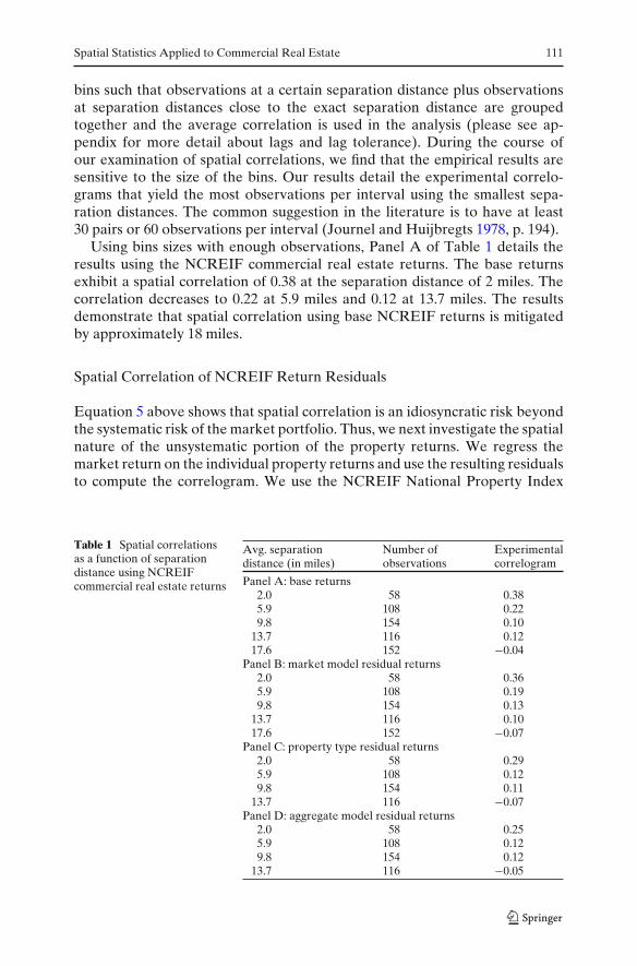
bins such that observations at a certain separation distance plus observationsat separation distances close to the exact separation distance are groupedtogether and the average correlation is used in the analysis (please see ap-pendix for more detail about lags and lag tolerance). During the course ofour examination of spatial correlations, we find that the empirical results aresensitive to the size of the bins. Our results detail the experimental correlo-grams that yield the most observations per interval using the smallest sepa-ration distances. The common suggestion in the literature is to have at least30 pairs or 60 observations per interval (Journel and Huijbregts 1978, p. 194).

Using bins sizes with enough observations, Panel A of Table 1 details theresults using the NCREIF commercial real estate returns. The base returnsexhibit a spatial correlation of 0.38 at the separation distance of 2 miles. Thecorrelation decreases to 0.22 at 5.9 miles and 0.12 at 13.7 miles. The resultsdemonstrate that spatial correlation using base NCREIF returns is mitigatedby approximately 18 miles.

Spatial Correlation of NCREIF Return Residuals

Equation 5 above shows that spatial correlation is an idiosyncratic risk beyondthe systematic risk of the market portfolio. Thus, we next investigate the spatialnature of the unsystematic portion of the property returns. We regress themarket return on the individual property returns and use the resulting residualsto compute the correlogram. We use the NCREIF National Property Index

Table 1 Spatial correlationsas a function of separationdistance using NCREIFcommercial real estate returns

Avg. separation Number of Experimentaldistance (in miles) observations correlogram

Panel A: base returns2.0 58 0.385.9 108 0.229.8 154 0.10

13.7 116 0.1217.6 152 −0.04

Panel B: market model residual returns2.0 58 0.365.9 108 0.199.8 154 0.13

13.7 116 0.1017.6 152 −0.07

Panel C: property type residual returns2.0 58 0.295.9 108 0.129.8 154 0.11

13.7 116 −0.07Panel D: aggregate model residual returns

2.0 58 0.255.9 108 0.129.8 154 0.12

13.7 116 −0.05


(NPI) as our proxy for the market portfolio.6 Both the overall model and theindividual beta estimate on the market portfolio are significant at the 5% level,however, the adjusted R2 is 0.01.

After controlling for the market return, we model the residual return corre-lations across separation distance. Panel B of Table 1 details the results. Thereis a slight reduction in the magnitude of the spatial correlations compared tothe base returns, however, the reduction is not dramatic.

Given that the market model is somewhat limited over the short sampleperiod, we investigate other determinants of real estate returns. The NCREIFdata include office, retail, multifamily, and industrial property types, therefore,we consider a model that controls for the four types since this variety of diversi-fication is well established in the literature. We also examine various economicvariables as well as proxies for size and quality. Insomuch as Wurtzebach(1988), Mueller and Ziering (1992), and Mueller (1993) find that economically-based diversification is preferable to purely geographic diversification, weincorporate the economic variables detailed by Mueller (1993) and Cheng andBlack (1998) in the following model.7

Ri,t = β0 + β1 · ln(AV ESQFT) + β2 · ln(NU MU NITS)

+ β3 · ln(MVLAST) + β4 · APT + β5 · IND + β6 · OFF ICE

+ β7 · RET AIL +12∑

j=8

β j · POP +20∑

k=13

βk · EMPLOY

+ β21 · RAT IO + β22 · MIG + εi,t

6In the spirit of Stambaugh (1982) we also examine using the global equity indices of RussellGlobal Index and MCSI World Index as a proxy for the market model. Despite the fact that theRussell Global Index is based upon approximately 10,000 global stocks or 98% of the investableglobal universe, we find that equities are not a significant fit for US commercial real estateproperties.7The economic variables control for aspects of the real estate demand curve (Miles et al. 2007,p. 26). Demand for retail space and apartments is a function of household composition andpopulation. Along with the overall population for a specific zip code, we break out populationby five age groups with breakpoints at 19, 34, 49, and 65, which is consistent with Cheng andBlack (1998). We execute the model with and without the breakpoints and find no differencein the results. We also include the demand-side variables of median income and average houseprice scaled by median household income. The demand for other commercial property—officebuildings, factories, and warehouses—is more closely tied to labor force and employment. Tocontrol for these effects along with the economically-based diversification noted in Mueller (1993)we use employment levels using the 2002 North American Industry Classification System codesof 1) mining and agriculture, 2) utilities and construction, 3) manufacturing, 4) wholesale andretail trade along with transportation and warehousing, 5) information, finance, insurance, realestate, and profession, scientific and technical services, 6) education and health care, and 7) arts,entertainment, and food services. Lastly, we account for changes in population and employmentusing the migration of persons into the zip code.


where

Ri,t the rate of return on the ith property for the tth quarter,AVESQFT average square feet,NUMUNITS average number of units, which is used by some apartment

complexes instead of the avesqft. measure,MVLAST average market value from t − 1 quarter,APT dichotomous variable equal to 1 if the property is an

apartment complex and 0 otherwise,IND dichotomous variable equal to 1 if the property is an industrial

building and 0 otherwise,OFFICE dichotomous variable equal to 1 if the property is an office

building and 0 otherwise,RETAIL dichotomous variable equal to 1 if the property is a retail

building and 0 otherwise,POP population as one continuous variable and divided into five

age groups,EMPLOY employment by industry,RATIO ratio of average house price to median household income, andMIG migration of persons into a zip code.

This specification explains more of the variation in property returns com-pared to the market model—the adjusted R2 is 0.15. Almost all of explanatorypower is due to the property-type variables. Each is significant with p-valuesless than 0.01. The only significant economic variable is migration with ap-value of 0.06.

As before, upon controlling for property type, employment, population,et cetera, we use the residuals to compute the correlogram. Panel C ofTable 1 details the results. Compared to the base returns in Panel A, thefindings in Panel C demonstrate a material reduction in residual correlationat most separation distances. Initial correlation decreases from 0.38 to 0.29.At 5.9 miles, residual correlation is 0.12 versus 0.22 using base returns. Also,the findings suggest that the point of randomness is found by 13.7 miles inseparation distance as compared to 17.6 miles using base returns.

Note that the residuals from a regression using returns as the dependentvariable can behave differently from a spatial perspective than just using theraw returns. As one extreme, if the correlations between property returns allstem from property type and economic variables, the resulting residuals willnot show any correlation over space. As another extreme, suppose that twocontiguous properties have almost perfect spatial dependence when control-ling for other factors, but each property has many other characteristics thatcause the returns to diverge. In this case, the raw returns will show a smallercorrelation than the residuals—which will display very high levels of spatialdependence. Consequently, controlling for various property characteristics canresult in residuals that display either lower or higher spatial dependence thanthe raw returns.


Given the success of property type to examine return correlation our lastspecification examines the market model along with property type and theeconomic variables. Modeling property returns using this aggregate model wefind that property-type variables are the main determinants of returns.

The results in Panel D of Table 1 detail the spatial correlations aftercontrolling for the various factors in the aggregate model. The findings inPanel D are similar to Panel C with a slight reduction in the initial residualcorrelation—from 0.29 to 0.25. As before, spatial correlation is mitigated ifproperties are separated by approximately 13 miles.

Apartment Cap Rates

The correlogram results thus far provide the benefits of examining diversifi-cation across property types and within a zip code submarket. However, aconcern of the NCREIF data is that the values are based on appraisals. Theuse of appraisals is a potential issue because empirical evidence suggests thatappraisals smooth changes in property values, which causes downward-biasedestimates of total return volatility (Geltner 1991).

To protect against the specific panel of data driving the results, we computecorrelograms based on cap rates of apartment complexes from January 2001 toDecember 2003. The cap rates offer another real estate measure using market-driven transaction prices. Further, the cap rates provide over one millionindividual pairs to compute the experimental correlogram, which allows us todetail smaller separation distances.

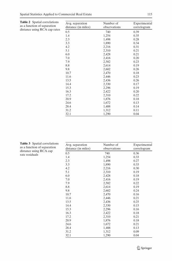
Table 2 presents the results of spatially modeling the base cap rates. Similarto the NCREIF results, the initial spatial correlation is 0.39. With more data,the results demonstrate a slower spatial correlation decay—correlation valuesof 0.18 extend out to approximately 21 miles. The results demonstrate that thebase cap rates obtain zero spatial correlation at approximately 32 miles.

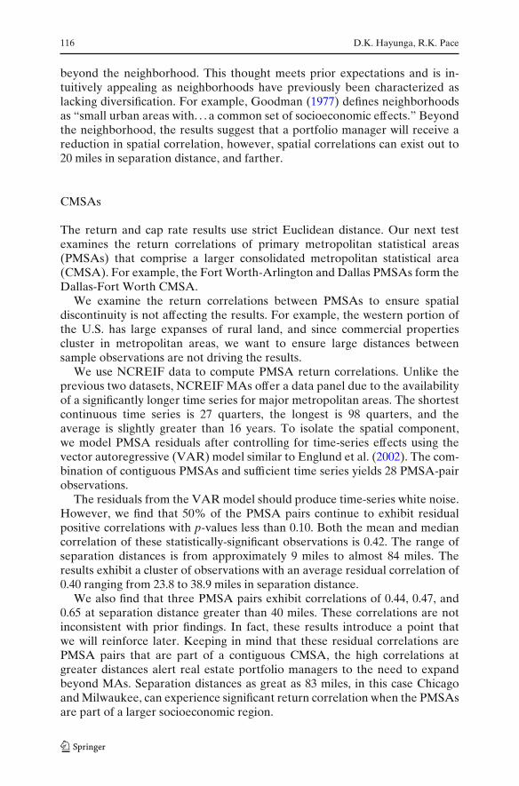
Similar to our treatment of the NCREIF returns, we next examine thespatial characteristics of cap rate residuals. We examine residual returns aftercontrolling for the building features of size, the number of units, and age.We do not examine the market model or economic variables with this datasetbecause the cap rates are a point-in-time measure resulting in insufficient datato estimate a market model for these returns.

Table 3 present the results after controlling for structural features. Overall,the residual results are quite similar to the base cap rates with slight reductionsin correlation at the same separation distances. The initial correlation is 0.36and the separation distance when spatial correlation is effectively mitigated isapproximately 32 miles.

To summarize the empirical results thus far, we find that for both NCREIFreturns and RCA cap rates the initial correlation is approximately 0.38. Addi-tionally, the greatest reduction in spatial correlation occurs at approximately5 miles. This distance is likely referencing the neighborhood submarket andsuggests a portfolio should realize diversification benefits by holding properties


Table 2 Spatial correlationsas a function of separationdistance using RCA cap rates


0.5 740 0.391.4 1,254 0.352.3 1,498 0.283.3 1,890 0.344.2 2,216 0.315.1 2,310 0.216.0 2,428 0.217.0 2,416 0.207.9 2,582 0.238.8 2,614 0.199.8 2,602 0.2610.7 2,470 0.1811.6 2,446 0.2313.5 2,436 0.2614.4 2,330 0.1715.3 2,296 0.1916.3 2,422 0.2017.2 2,310 0.2220.9 1,876 0.1824.6 1,672 0.1328.4 1,488 0.1431.2 1,312 0.1132.1 1,290 0.04

Table 3 Spatial correlationsas a function of separationdistance using RCA caprate residuals


0.5 740 0.361.4 1,254 0.332.3 1,498 0.273.3 1,890 0.334.2 2,216 0.305.1 2,310 0.196.0 2,428 0.187.0 2,416 0.197.9 2,582 0.228.8 2,614 0.199.8 2,602 0.2410.7 2,470 0.1611.6 2,446 0.2113.5 2,436 0.2514.4 2,330 0.1515.3 2,296 0.1616.3 2,422 0.1817.2 2,310 0.2120.9 1,876 0.1824.6 1,672 0.2128.4 1,488 0.1331.2 1,312 0.0932.1 1,290 0.04


beyond the neighborhood. This thought meets prior expectations and is in-tuitively appealing as neighborhoods have previously been characterized aslacking diversification. For example, Goodman (1977) defines neighborhoodsas “small urban areas with. . . a common set of socioeconomic effects.” Beyondthe neighborhood, the results suggest that a portfolio manager will receive areduction in spatial correlation, however, spatial correlations can exist out to20 miles in separation distance, and farther.

CMSAs

The return and cap rate results use strict Euclidean distance. Our next testexamines the return correlations of primary metropolitan statistical areas(PMSAs) that comprise a larger consolidated metropolitan statistical area(CMSA). For example, the Fort Worth-Arlington and Dallas PMSAs form theDallas-Fort Worth CMSA.

We examine the return correlations between PMSAs to ensure spatialdiscontinuity is not affecting the results. For example, the western portion ofthe U.S. has large expanses of rural land, and since commercial propertiescluster in metropolitan areas, we want to ensure large distances betweensample observations are not driving the results.

We use NCREIF data to compute PMSA return correlations. Unlike theprevious two datasets, NCREIF MAs offer a data panel due to the availabilityof a significantly longer time series for major metropolitan areas. The shortestcontinuous time series is 27 quarters, the longest is 98 quarters, and theaverage is slightly greater than 16 years. To isolate the spatial component,we model PMSA residuals after controlling for time-series effects using thevector autoregressive (VAR) model similar to Englund et al. (2002). The com-bination of contiguous PMSAs and sufficient time series yields 28 PMSA-pairobservations.

The residuals from the VAR model should produce time-series white noise.However, we find that 50% of the PMSA pairs continue to exhibit residualpositive correlations with p-values less than 0.10. Both the mean and mediancorrelation of these statistically-significant observations is 0.42. The range ofseparation distances is from approximately 9 miles to almost 84 miles. Theresults exhibit a cluster of observations with an average residual correlation of0.40 ranging from 23.8 to 38.9 miles in separation distance.

We also find that three PMSA pairs exhibit correlations of 0.44, 0.47, and0.65 at separation distance greater than 40 miles. These correlations are notinconsistent with prior findings. In fact, these results introduce a point thatwe will reinforce later. Keeping in mind that these residual correlations arePMSA pairs that are part of a contiguous CMSA, the high correlations atgreater distances alert real estate portfolio managers to the need to expandbeyond MAs. Separation distances as great as 83 miles, in this case Chicagoand Milwaukee, can experience significant return correlation when the PMSAsare part of a larger socioeconomic region.


Residential Property

In addition to multiple commercial property databases and attributes, weexamine the impact of residential property on the spatial aspects of commercialproperty. While most commercial real estate investment portfolios will notincorporate residential property, local housing markets can serve as a proxy forphenomena that also affect the behavior of commercial property. Additionally,residential returns can provide a better proxy for the market model thanthe NPI index in the previous section since residential returns are specificto the local market and are subject to similar real estate supply and demandfunctions. The standard spatial equilibrium model in urban economics predictssimilar longer-run movements in different real estate sectors because each isdriven by common fundamentals (Rosen 1979; Roback 1982). We examineresidential returns in this section and then combine commercial and residentialdata types in the next section.

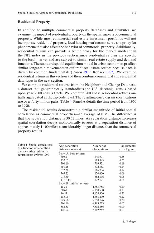
We compute residential returns from the Neighborhood Change Database,a dataset that geographically standardizes the U.S. decennial census basedupon year 2000 census tracts. We compute 9000 base residential returns ini-tially aggregated at the zip code level. The resulting correlogram specificationsuse over forty million pairs. Table 4, Panel A details the time period from 1970to 1990.

The residential results demonstrate a similar magnitude of initial spatialcorrelation as commercial properties—an average of 0.35. The difference isthat the separation distance is 30.61 miles. As separation distance increasesspatial correlation decays monotonically to zero at a separation distance ofapproximately 1,100 miles; a considerably longer distance than the commercialproperty results.

Table 4 Spatial correlationsas a function of separationdistance using residentialreturns from 1970 to 1990


Panel A: base returns30.61 345,901 0.35153.05 513,825 0.35306.10 709,321 0.19459.15 832,363 0.14612.20 816,794 0.12765.25 670,650 0.09918.30 652,836 0.061,010.13 722,171 0.01

Panel B: residual returns15.31 4,783,788 0.1930.61 6,198,538 0.1776.53 4,178,956 0.22153.05 4,888,290 0.22229.58 5,898,176 0.20306.10 6,483,273 0.07382.63 7,302,486 0.09428.54 7,112,267 0.03


Similar to commercial returns, it is reasonable to expect that there existobservable determinants that explain a portion of the correlation. Thus, weregress the base residential returns by some typical determinants of housingprices. As expected, all independent variables are statistically significant at the5% level. The specification is

Ri,t = β0 + β1 · ln(EDUC12) + β2 · ln(EDUC16) + β3 · ln(HOMEPOP)

+ β4 · ln(INCOME) + β5 · ln(SI Z E) + β6 · ln(BLT OC70)

+ β7 · ln(BLT OC59) + β8 · ln(BLT OC49) + β9 · ln(BLT OC39) + εi,t,

where

Ri the rate of return on the ith house,EDUC12 persons 25 years old or older who completed high school,EDUC16 persons 25 years old or older who completed college,HOMEPOP number of persons 25 years old or older,INCOME average family income,SIZE aggregate number of rooms in the home, andBLTOC total occupied housing units built up to the year specified in

the variable.

Using the residuals, we compute the return correlations for each observa-tion within census tracts. The residuals are not aggregated across zip codesbut left within census tracts since each observation is the remaining portionnot explained by the model, and, thus, is unique information. This methodproduces millions of observations within each bin.

Table 4, Panel B details the residential residual returns findings. At theshortest separation distance of 15.31 miles, the initial spatial correlation is 0.19.This magnitude of spatial correlation persists out to approximately 230 miles.While the degree of spatial correlation is not surprising, it is important tonote that, using on millions of observations, residential properties extending150–225 miles in separation distance demonstrate an empirical correlation ofroughly 0.20.

Combining Commercial and Residential Types

Given the voluminous amount of data available for residential real estate, weexamine the effect of including the residential property type in the commer-cial analysis. Inclusion in the correlogram is based upon the rationale thatcommercial and residential markets are affected by similar socioeconomicconditions at common locations. Another argument comes from the krigingspatial literature (see Goovaerts 1997, pp. 185–258). The reasoning follows thatif the secondary residential returns are correlated with the primary commercialreturns, then one can utilize observations at sites where they are both recordedto estimate this correlation. Hence, we match residential returns by locationand include them as an explanatory variable in the NCREIF commercial


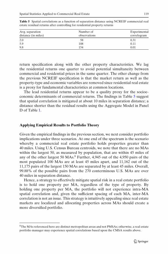
Table 5 Spatial correlations as a function of separation distance using NCREIF commercial realestate residual returns after controlling for residential property returns


2.0 58 0.315.9 108 0.119.8 154 0.01

return specification along with the other property characteristics. We lagthe residential returns one quarter to avoid potential simultaneity betweencommercial and residential prices in the same quarter. The other change fromthe previous NCREIF specification is that the market return as well as theproperty-type and economic variables are removed since residential real estateis a proxy for fundamental characteristics at common locations.

The lead residential returns appear to be a quality proxy for the socioe-conomic determinants of commercial returns. The findings in Table 5 suggestthat spatial correlation is mitigated at about 10 miles in separation distance; adistance shorter than the residual results using the Aggregate Model in PanelD of Table 1.

Applying Empirical Results to Portfolio Theory

Given the empirical findings in the previous section, we next consider portfolioimplications under three scenarios. At one end of the spectrum is the scenariowhereby a commercial real estate portfolio holds properties greater than40 miles. Using U.S. Census Bureau centroids, we note that there are no MAswithin the largest 50, as measured by population, that are within 45 miles ofany of the other largest 50 MAs.8 Further, 4,945 out of the 4,950 pairs of themost populated 100 MAs are at least 45 miles apart, and 11,162 out of the11,175 pairs of the largest 150 MAs are separated by at least 45 miles. Overall,99.88% of the possible pairs from the 270 conterminous U.S. MAs are over40 miles in separation distance.

Hence, a strategy to effectively mitigate spatial risk in a real estate portfoliois to hold one property per MA, regardless of the type of property. Byholding one property per MA, the portfolio will not experience intra-MAspatial correlation and, given the sufficient spacing of each MA, inter-MAcorrelation is not an issue. This strategy is intuitively appealing since real estatemarkets are localized and allocating properties across MAs should create amore diversified portfolio.

8The MAs referenced here are distinct metropolitan areas and not PMSAs; otherwise, a real estateportfolio manager may experience spatial correlations based upon the CMSA results above.


To examine this strategy further and based upon a reviewer’s comments,we execute another test using the NCREIF data from Table 1. Instead ofmodeling residuals after controlling the market return, property-type, ordemand variables, we spatially model residuals after controlling for the un-conditional average for an entire metro area. For continuity, we maintain thesame separation distances as in Table 1. The results (not tabled) demonstratethat properties within the first two bins and separated by 2 and 5.9 miles,respectively, yield spatial correlations of approximately 0.14. After 5.9 miles,the spatial correlation is mitigated. These results reinforce two main points ofthis paper: (i) adjacent or juxtaposed properties will experience neighborhoodand MA socioeconomic factors that are difficult to diversify, and (ii) uniqueMAs appear to be sufficient for portfolio diversification as the unconditionalMA average is effective in removing correlation for distances beyond a neigh-borhood submarket.

Note, however, that a strategy of one property per MA is not macro-consistent. The design implies an equal weighting across MAs and not alllarge-scale real estate portfolios can hold one property per MA due to a lackof acceptable properties in mid- to small-sized MAs. For example, the largest16 MAs in the third quarter of 2002 comprised 68.9% of the total propertiesreported to NCREIF. The largest 35 MAs held 85.0% of the NCREIF propertycounts.

Intra-MA portfolio

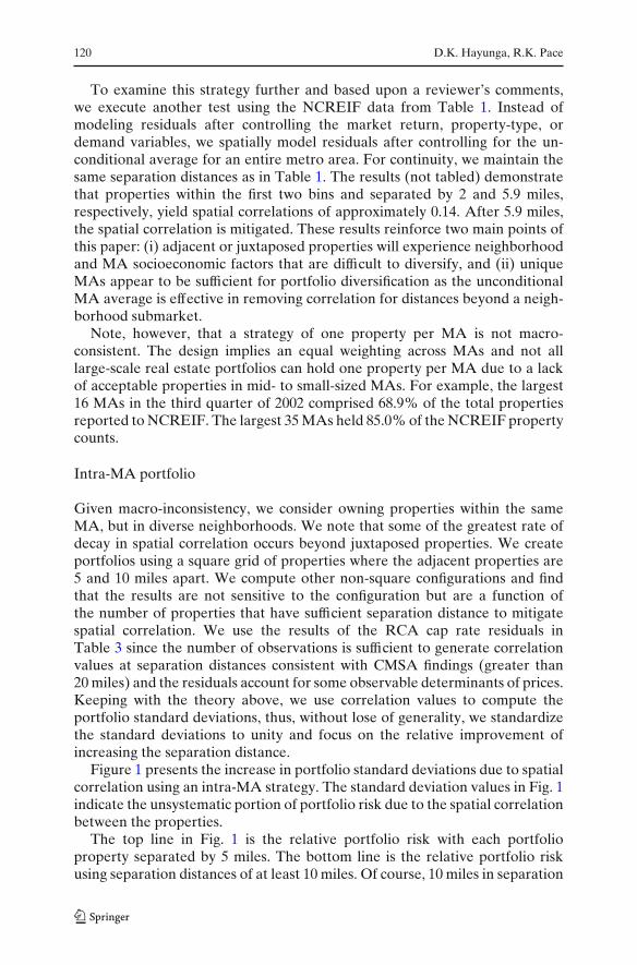
Given macro-inconsistency, we consider owning properties within the sameMA, but in diverse neighborhoods. We note that some of the greatest rate ofdecay in spatial correlation occurs beyond juxtaposed properties. We createportfolios using a square grid of properties where the adjacent properties are5 and 10 miles apart. We compute other non-square configurations and findthat the results are not sensitive to the configuration but are a function ofthe number of properties that have sufficient separation distance to mitigatespatial correlation. We use the results of the RCA cap rate residuals inTable 3 since the number of observations is sufficient to generate correlationvalues at separation distances consistent with CMSA findings (greater than20 miles) and the residuals account for some observable determinants of prices.Keeping with the theory above, we use correlation values to compute theportfolio standard deviations, thus, without lose of generality, we standardizethe standard deviations to unity and focus on the relative improvement ofincreasing the separation distance.

Figure 1 presents the increase in portfolio standard deviations due to spatialcorrelation using an intra-MA strategy. The standard deviation values in Fig. 1indicate the unsystematic portion of portfolio risk due to the spatial correlationbetween the properties.

The top line in Fig. 1 is the relative portfolio risk with each portfolioproperty separated by 5 miles. The bottom line is the relative portfolio riskusing separation distances of at least 10 miles. Of course, 10 miles in separation


4 9 16 25 36 49 64 81 100 121 1440

0.1

0.2

0.3

0.4

0.5

0.6

0.7

0.8

N

σp

Fig. 1 Portfolio standard deviation as a function of the number of real estate properties ifa portfolio holds intra-MA properties only. Values demonstrate the increase in unsystematicportfolio risk due to the average spatial correlation between portfolio properties. The top linemarked with stars represents a portfolio with at least 5 miles of separation distances betweenproperties. Using diamond markers, the bottom line is the additional unsystematic risk withproperties separated by at least 10 miles. The values not connected by a line use properties with10 miles of separation distance, which require MSAs larger than exist in the US

distance decreases unsystematic risk, although the reduction is not as greatfor smaller portfolios (i.e., 4 or 9 properties) as it is for portfolios of 25 or36 properties. We extend the values of the 10-mile portfolio (unconnecteddiamonds) for reference purposes. These portfolio are unfeasible as there areno MAs large enough to hold the number of properties each 10 miles apart.

Both graphed scenarios in Fig. 1 demonstrate that there is practical limitfor reducing intra-MA unsystematic risk—no matter the size of the portfolio,lingering spatial risk will be present since properties are not sufficiently sepa-rated.9 Although not graphed, we find that portfolios with properties separatedby 15 or 20 miles still experience unsystematic spatial risk. Thus, no amount ofintra-MA diversification will entirely mitigate spatial portfolio risk.

Value-weighted portfolio

As a final scenario, we envision holding a few properties within an MA overa small number of MAs. This strategy yields a value-weighted portfolio that

9Additionally, the values do not account for levered cash flows, which will increase portfolio risk.


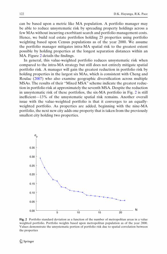
can be based upon a metric like MA population. A portfolio manager maybe able to reduce unsystematic risk by spreading property holdings across afew MAs without incurring exorbitant search and portfolio management costs.Hence, we build real estate portfolios holding 25 properties using portfolioweighting based upon Census populations as of the year 2000. We assumethe portfolio manager mitigates intra-MA spatial risk to the greatest extentpossible by holding properties at the longest separation distances within anMA. Figure 2 details the findings.

In general, this value-weighted portfolio reduces unsystematic risk whencompared to the intra-MA strategy but still does not entirely mitigate spatialportfolio risk. A manager will gain the greatest reduction in portfolio risk byholding properties in the largest six MAs, which is consistent with Cheng andRoulac (2007) who also examine geographic diversification across multipleMSAs. The results of their “Mixed MSA” scheme indicate the greatest reduc-tion in portfolio risk at approximately the seventh MSA. Despite the reductionin unsystematic risk of these portfolios, the six-MA portfolio in Fig. 2 is stillinefficient—13% of the unsystematic spatial risk remains. Another overallissue with the value-weighted portfolio is that it converges to an equally-weighted portfolio. As properties are added, beginning with the nine-MAportfolio, the next new city adds one property that is taken from the previouslysmallest city holding two properties.

5 10 15 200.00

0.05

0.10

0.15

0.20

0.25

0.30

0.35

N

Fig. 2 Portfolio standard deviation as a function of the number of metropolitan areas in a valueweighted portfolio. Portfolio weights based upon metropolitan population as of the year 2000.Values demonstrate the unsystematic portion of portfolio risk due to spatial correlation betweenthe properties


In summary, the three scenarios (one property per MSA, all properties inone MSA, and value weighted) demonstrate that spatial correlation in realestate portfolios is different than traditional finance models using nonspa-tial financial assets. Whereas unsystematic risk is reduced in the standardfinance textbook as more less-than-perfectly-correlated stocks are added toan equity portfolio, real estate portfolios are inefficient if they hold multipleproperties within a localized market such as a neighborhood or MA. Sinceno amount of intra-MA diversification will produce an efficient portfolio, aportfolio manager directly investing in real estate assets must look to inter-MA diversification.

Conclusion

Real estate is a field built on the notion of location, yet the literature has notemployed formal spatial techniques to examine the effects of geography oncommercial property portfolios. Consistent with the importance of locationon commercial property prices, we use spatial statistics to quantify the spatialcorrelation between commercial real estate properties. Understanding thespatial component within a commercial portfolio is essential since fundamentalportfolio theory shows that spatial correlation is an unsystematic risk thatshould not be compensated by the market.

Using return and cap rate data, this paper examines the magnitude of initialspatial correlation, spatial correlation as a function of separation distance,and the distances of separation between commercial properties needed toessentially eliminate spatial dependence. With respect to the initial correlationof nearby properties, we find that base commercial real estate returns and caprates exhibit correlation values ranging from 0.31 to 0.39 over a separationdistance from 1/2 to 2 miles. As separation distances increase, spatial cor-relations decrease but maintain magnitudes over 0.10 out to approximately30 miles, depending upon the dataset. The average correlation drops to zero atseparation distances generally beyond 45 miles.

These findings, combined with intra-MA simulations, suggest that inter-neighborhood diversification is helpful in moving towards efficient portfolios.However, no amount of intra-MA diversification will entirely dispose of spatialportfolio risk. To effectively diversify, real estate portfolios require inter-MAdiversification with the most beneficial diversification strategy being one prop-erty per MA regardless of the type of property. But inter-MA diversificationhas its limits as, by one NCREIF measure, 69% of the portfolio-quality realestate is concentrated in the largest 16 MAs. There are not enough qualifyingproperties for all real estate portfolios to hold an equally-weighted portfolio.

The results suggest that combining intra-MA and inter-MA properties is oneof the best strategies for reducing the unsystematic spatial risk while trading offthe portfolio management costs of holding geographically-diverse properties.The fact that this combination portfolio still does not eliminate spatial portfoliorisk provides motivation for using international direct-real estate holdings and


indirect real estate investments in portfolios. A further consideration of theresults of this study is to apply the correlations found here in a constrainedoptimization framework that determines the trade-off between diversificationand increased portfolio management costs.

References

Basu, S., & Thibodeau, T. (1998). Analysis of spatial autocorrelation in house prices. Journalof Real Estate Finance and Economics, 17, 61–85.

Blume, M. (1971). On the assessment of risk. Journal of Finance, 26(1), 1–10.Cheng, P., & Black, R. (1998). Geographic diversification and economic fundamentals in apart-

ment markets: A demand perspective. Journal of Real Estate Portfolio Management, 4(2),93–105.

Cheng, P., & Roulac, S. (2007). Measuring the effectiveness of geographical diversification. Journalof Real Estate Portfolio Management, 13(1), 29–44.

Copeland, T., Weston, J., & Shastri, K. (2005). Financial theory and corporate policy. Reading:Pearson Addison Wesley.

Cressie, N. (1993). Statistics for spatial data. New York: Wiley.Dubin, R. (1998). Predicting house prices using multiple listings data. Journal of Real Estate

Finance and Economics, 17, 35–59.Dubin, R., Pace, R. K., & Thibodeau, T. (1999). Spatial autoregression techniques for real estate

data. Journal of Real Estate Literature, 7, 79–95.Englund, P., Hwang, M., & Quigley, J. (2002). Hedging housing risk. The Journal of Real Estate

Finance and Economics, 24(1–2), 167–200.Fama, E. (1976). Foundations of finance. New York: Basic Books.Fik, T., Ling, D., & Mulligan, G. (2003) Modeling spatial variation in housing prices: A variable

interaction approach. Real Estate Economics, 31(4), 623–646.Geltner, D. (1991). Smoothing in appraisal-based returns. Journal of Real Estate Finance and

Economics, 4, 327–345.Goetzmann, W., & Wachter, S. (1995). Clustering methods for real estate portfolios. Real Estate

Economics, 23(3), 271–310.Goodman, A. (1977). Comparison of block group and census tract data in a hedonic housing price

model. Land Economics, 53, 483–487.Goovaerts, P. (1997). Geostatistics for natural resources evaluation. Oxford: Oxford University

Press.Hartzell, D., Hekman, J., & Miles, M. (1986). Diversification categories in investment real estate.

AREUEA Journal, 14(2), 230–254.Hartzell, D., Shulman, D., & Wurtzebach, C. (1987). Refining the analysis of regional diversifica-

tion for income-producing real estate. Journal of Real Estate Research, 2(2), 85–95.Journel, A., & Huijbregts, C. (1978). Mining geostatistics. New York: Academic.LeSage, J., & Pace, R. K. (2009). Introduction to spatial econometrics. Boca Raton: CRC.Lintner, J. (1965). The valuation of risk assets and the selection of risky investments in stock

portfolios and capital budgets. Review of Economics and Statistics, 47, 13–37.Markowitz, H. (1952). Portfolio selection. Journal of Finance, 7(1), 77–91.Miles, M., Berens, G., Eppli, M., & Weiss, M. (2007). Real estate development. Washington, DC:

Urban Land Institute.Miles, M., & McCue, T. (1982). Historic returns and institutional real estate portfolios. AREUEA

Journal, 10(2), 184–198.Mueller, G. (1993). Refining economic diversification strategies for real estate portfolios. Journal

of Real Estate Research, 8(1), 55–68.Mueller, G., & Ziering, B. (1992). Real estate portfolio diversification using economic diversifica-

tion. Journal of Real Estate Research, 7(4), 375–386.Nelson, T., & Nelson, S. (2003). Regional models for portfolio diversification. Journal of Real

Estate Portfolio Management, 9(1), 71–88.


Radner, R., & Stiglitz, J. (1984). A nonconcavity in the value of information. In M. Boyer, &R. Khilstrom (Eds.), Bayesian models in economic theory. New York: Elsevier.

Roback, J. (1982). Wages, rents, and the quality of life. Journal of Political Economy, 90(4), 1257–1278.

Rosen, S. (1979). Wage-based indexes of urban quality of life. In P. Mieszkowski, & M. Straszheim(Eds.), Current issues in urban economics. Baltimore: Johns Hopkins University Press.

Roulac, S. (1976). Can real estate returns outperform common stocks? Journal of PortfolioManagement, 2(2), 26–43.

Sharpe, W. (1963). A simplified model for portfolio analysis. Management Science, 9(2), 277–293.Sharpe, W. (1964). Capital asset prices: A theory of market equilibrium under conditions of risk.

Journal of Finance, 19(3), 425–442.Snyder, J., & Voxland, P. (1989). An album of map projections. Washington, DC: US Government

Printing Office.Stambaugh, R. (1982). On the exclusion of assets from tests of the two-parameter model: A

sensitivity analysis. Journal of Financial Economics, 10(3), 237–268.Van Nieuwerburgh, S., & Veldkamp, L. (2007). Information acquisition and under-diversification.

NYU working paper. New York: NYU.Williams, J. (1996). Real estate portfolio diversification and performance of the twenty largest

MSAs. Journal of Real Estate Portfolio Management, 2(1), 19–30.Wolverton, M., Cheng, P., & Hardin, W. (1998). Real estate risk reduction through intracity

diversification. Journal of Real Estate Portfolio Management, 4(1), 35–41.Wurtzebach, C. (1988). The portfolio construction process. Parsippany: Prudential Real Estate

Investors.

Copyright of Journal of Real Estate Finance & Economics is the property of Springer Science & Business

Media B.V. and its content may not be copied or emailed to multiple sites or posted to a listserv without the

copyright holder's express written permission. However, users may print, download, or email articles for

individual use.

spatial statistics applied to commercial real estate statistics applied to commercial real estate...

Documents