applied statistics lecture_4
TRANSCRIPT
Introduction to applied statistics
& applied statistical methods
Prof. Dr. Chang Zhu 1
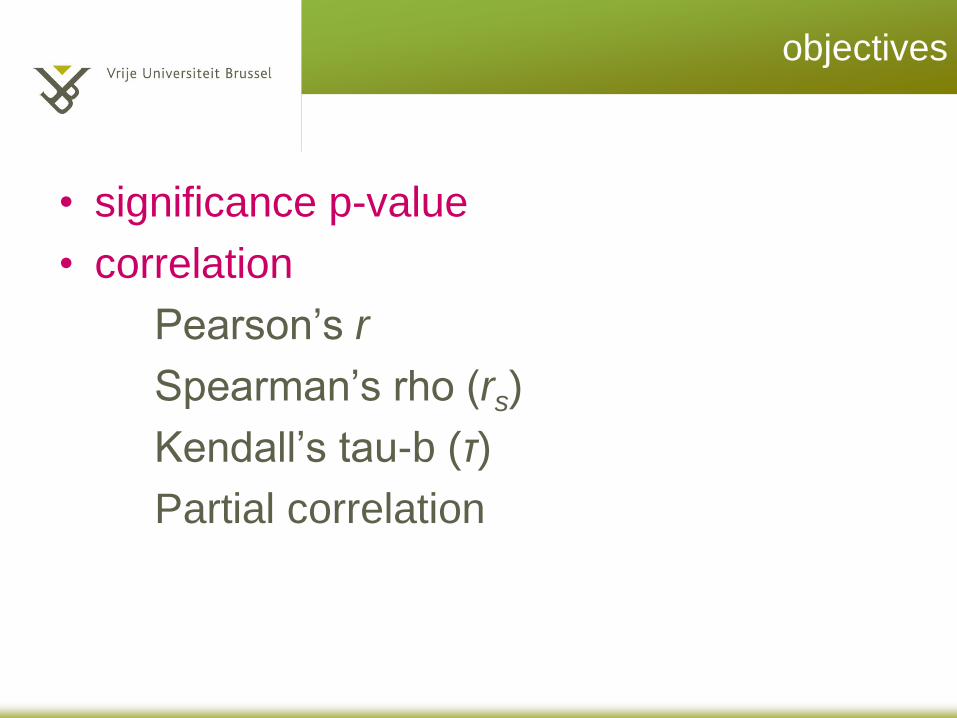
objectives
• significance p-value
• correlation
Pearson’s r
Spearman’s rho (rs)
Kendall’s tau-b (τ)
Partial correlation
significance – p value
• Read section 2.1 in the WIKI
• Open the section Assessment
• Work with your friends to do Revision 1
3
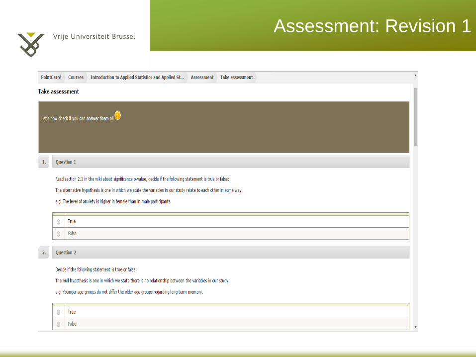
Assessment: Revision 1
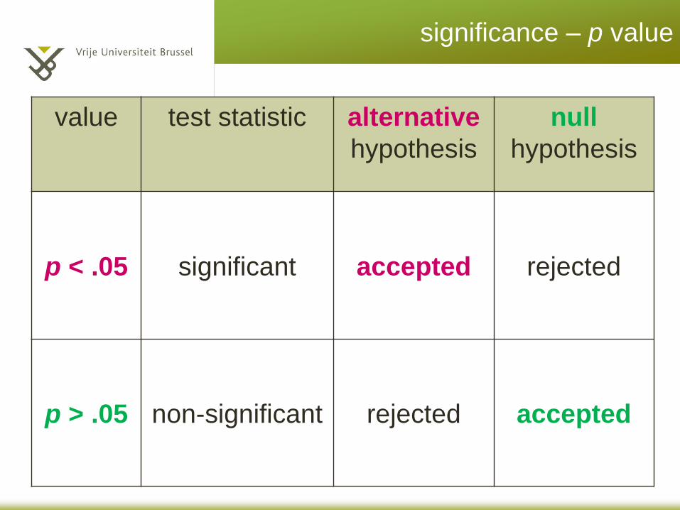
significance – p value
value test statistic alternative
hypothesis
null
hypothesis
p < .05
significant
accepted
rejected
p > .05
non-significant
rejected
accepted
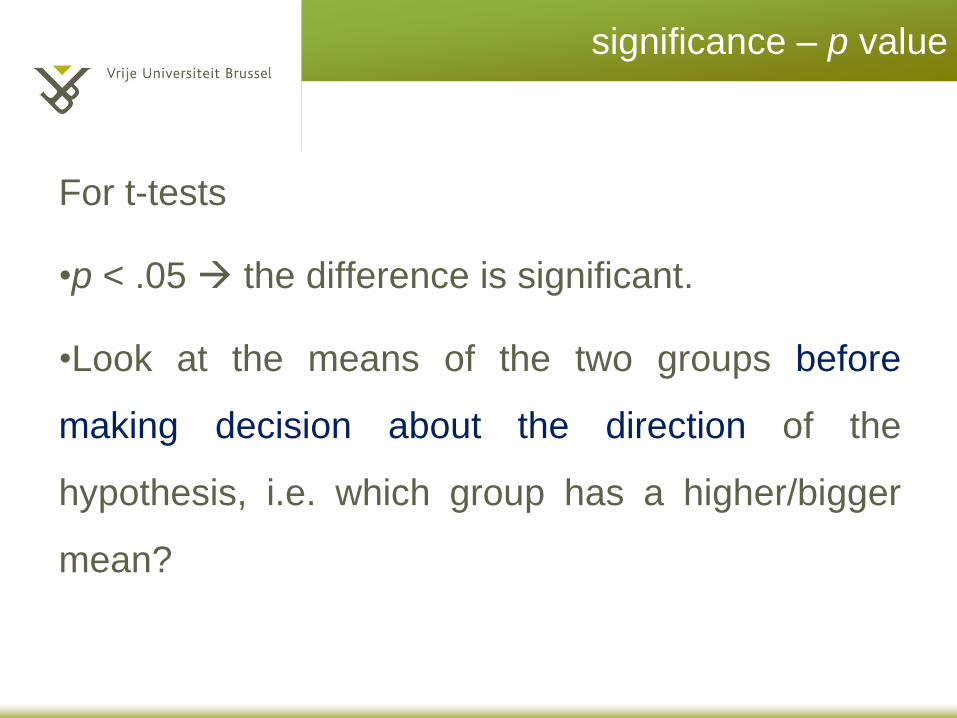
significance – p value
For t-tests
•p < .05 the difference is significant.
•Look at the means of the two groups before
making decision about the direction of the
hypothesis, i.e. which group has a higher/bigger
mean?
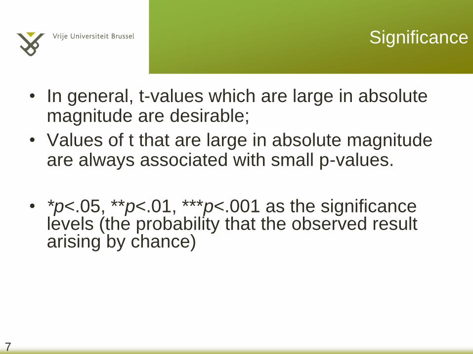
Significance
• In general, t-values which are large in absolute magnitude are desirable;
• Values of t that are large in absolute magnitude are always associated with small p-values.
• *p<.05, **p<.01, ***p<.001 as the significance levels (the probability that the observed result arising by chance)
7
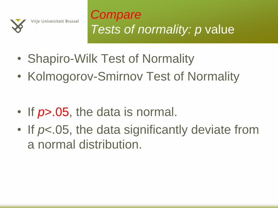
Compare
Tests of normality: p value
• Shapiro-Wilk Test of Normality
• Kolmogorov-Smirnov Test of Normality
• If p>.05, the data is normal.
• If p<.05, the data significantly deviate from
a normal distribution.
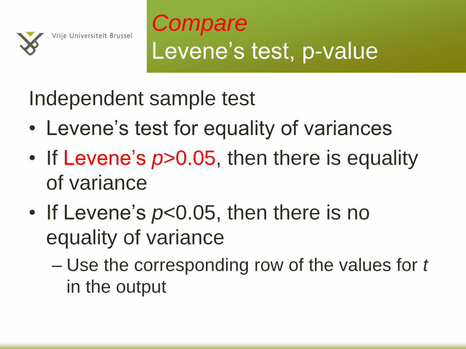
Compare
Levene’s test, p-value
Independent sample test
• Levene’s test for equality of variances
• If Levene’s p>0.05, then there is equality
of variance
• If Levene’s p<0.05, then there is no
equality of variance
– Use the corresponding row of the values for t
in the output
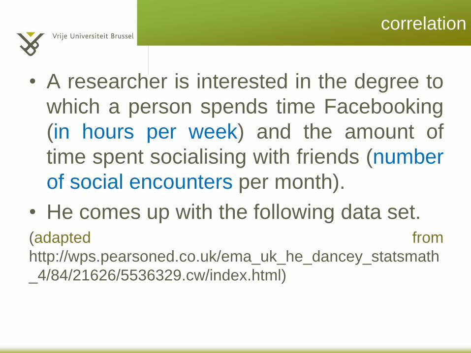
correlation
• A researcher is interested in the degree to
which a person spends time Facebooking
(in hours per week) and the amount of
time spent socialising with friends (number
of social encounters per month).
• He comes up with the following data set. (adapted from
http://wps.pearsoned.co.uk/ema_uk_he_dancey_statsmath
_4/84/21626/5536329.cw/index.html)
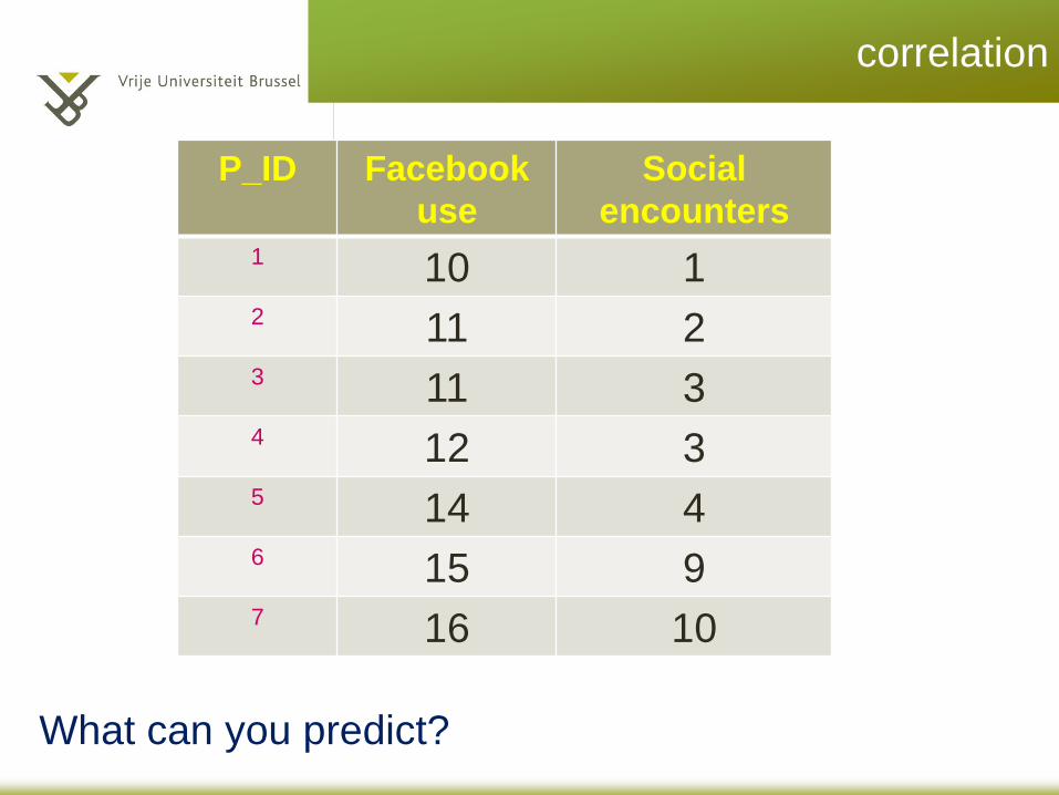
P_ID Facebook
use
Social
encounters
1 10 1 2 11 2 3 11 3 4 12 3 5 14 4 6 15 9 7 16 10
correlation
What can you predict?
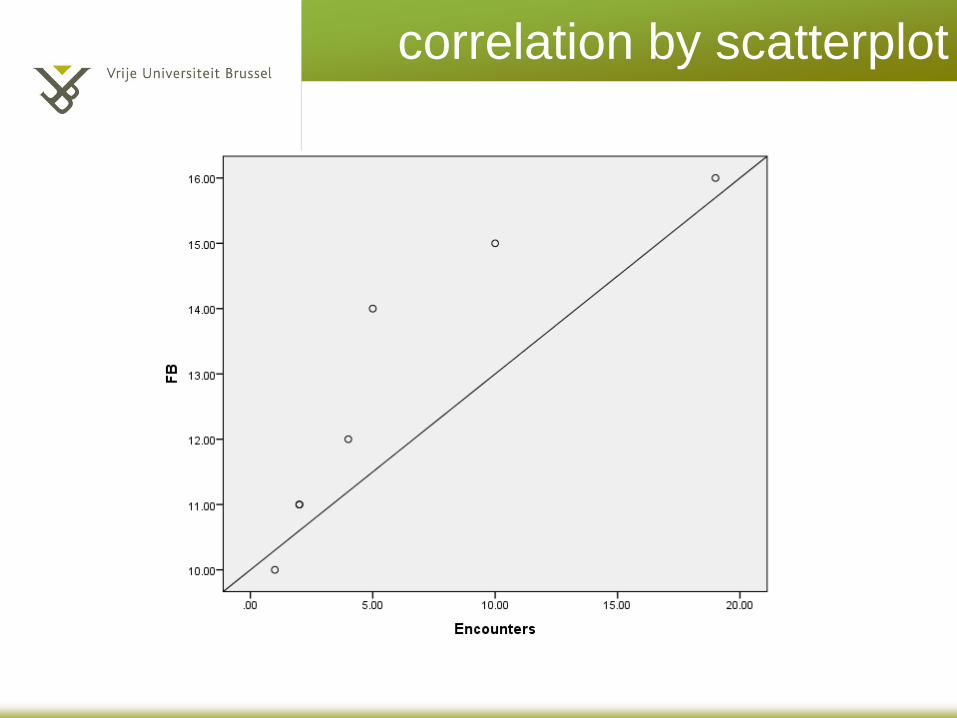
correlation by scatterplot
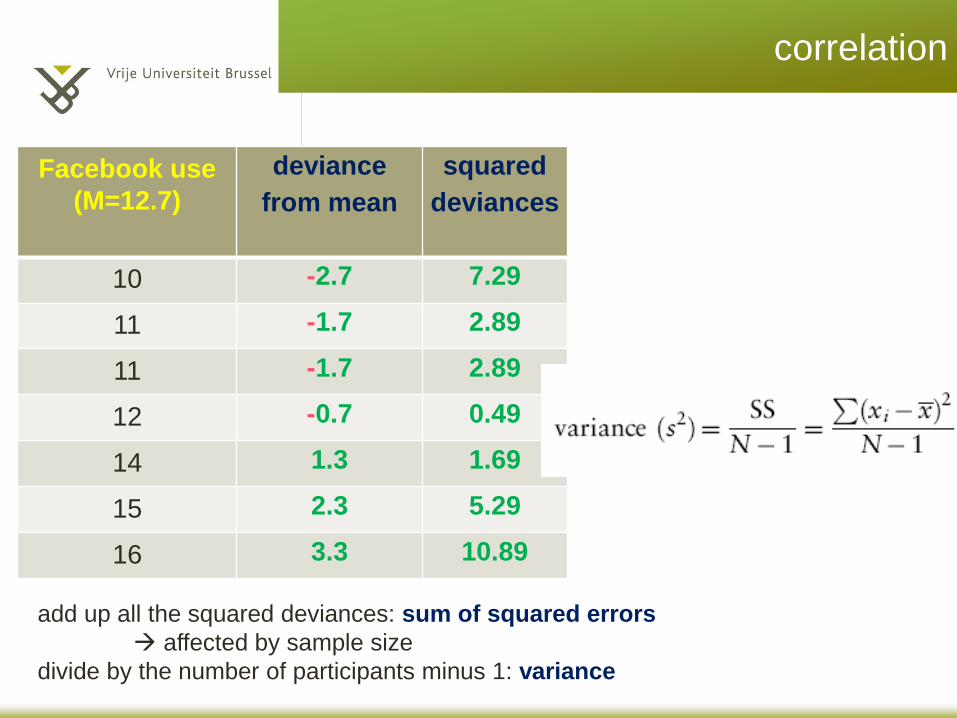
Facebook use
(M=12.7)
deviance
from mean
squared
deviances
10 -2.7 7.29
11 -1.7 2.89
11 -1.7 2.89
12 -0.7 0.49
14 1.3 1.69
15 2.3 5.29
16 3.3 10.89
correlation
add up all the squared deviances: sum of squared errors
affected by sample size
divide by the number of participants minus 1: variance
FB_use
(M=12.7) deviance
squared
deviances
social
encounters
(M=6.14)
deviance squared
deviances
10 -2.7 7.29 1 -5.14 26.42
11 -1.7 2.89 2 -4.14 17.14
11 -1.7 2.89 3 -3.14 9.86
12 -0.7 0.49 3 -3.14 9.86
14 1.3 1.69 4 -2.14 4.58
15 2.3 5.29 9 2.86 8.18
16 3.3 10.89 10 3.86 14.90
correlation
• covariance: averaged sum
of combined deviations
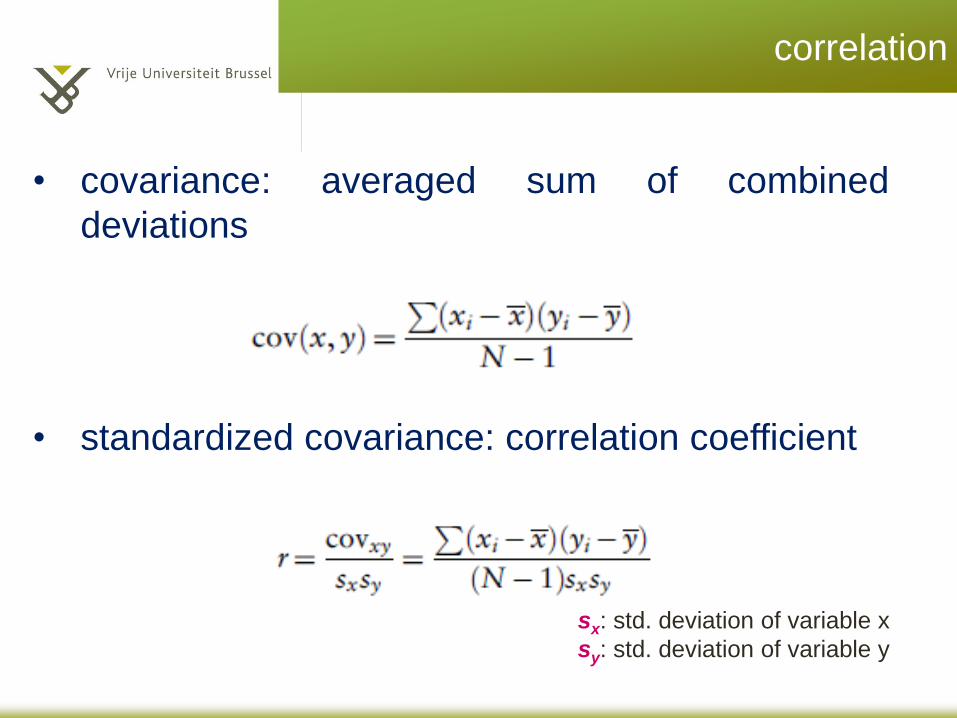
correlation
• covariance: averaged sum of combined
deviations
• standardized covariance: correlation coefficient
sx: std. deviation of variable x
sy: std. deviation of variable y
correlation
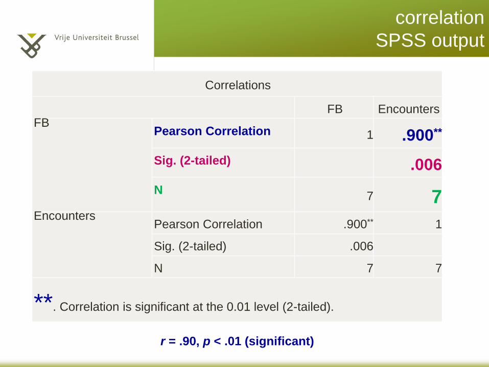
SPSS output
Correlations
FB Encounters FB
Pearson Correlation 1 .900**
Sig. (2-tailed) .006
N 7 7
Encounters Pearson Correlation .900** 1
Sig. (2-tailed) .006
N 7 7
**. Correlation is significant at the 0.01 level (2-tailed).
r = .90, p < .01 (significant)
Correlation
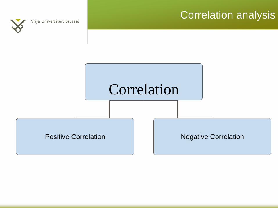
Positive Correlation Negative Correlation
Correlation analysis
correlation
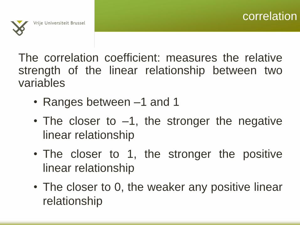
The correlation coefficient: measures the relative strength of the linear relationship between two variables
• Ranges between –1 and 1
• The closer to –1, the stronger the negative
linear relationship
• The closer to 1, the stronger the positive
linear relationship
• The closer to 0, the weaker any positive linear
relationship
A perfect positive correlation
Height
Weight
Height of A
Weight of A
Height of B
Weight of B
A linear relationship
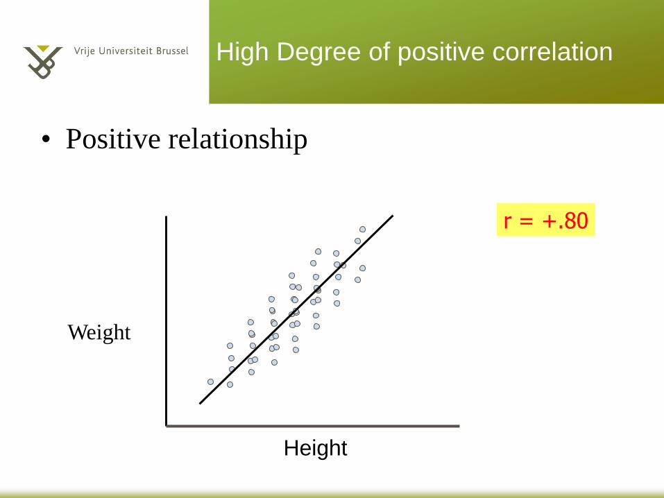
High Degree of positive correlation
• Positive relationship
Height
Weight
r = +.80
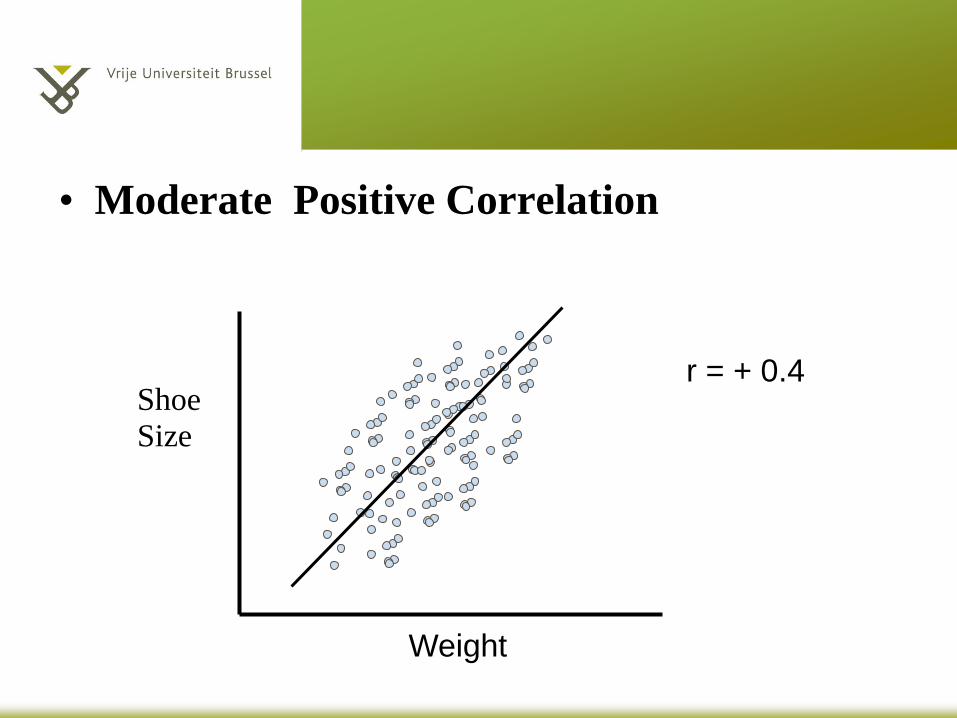
• Moderate Positive Correlation
Weight
Shoe
Size
r = + 0.4
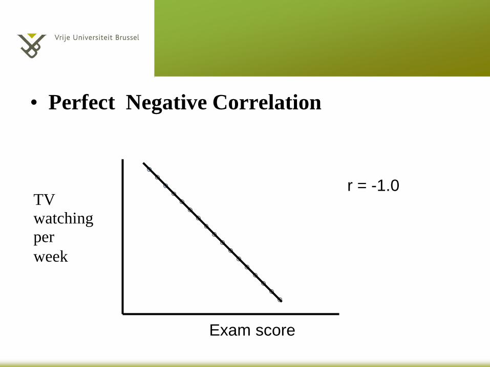
• Perfect Negative Correlation
Exam score
TV
watching
per
week
r = -1.0
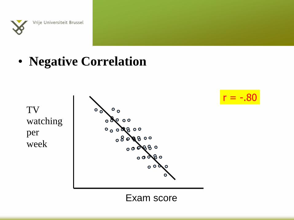
• Negative Correlation
Exam score
TV
watching
per
week
r = -.80
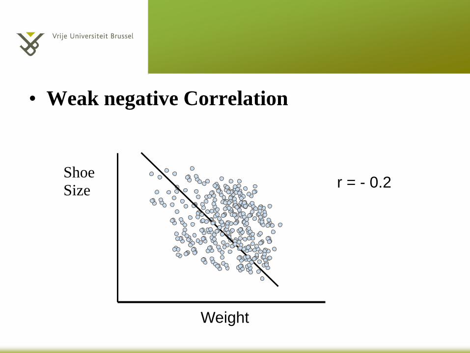
• Weak negative Correlation
Weight
Shoe
Size r = - 0.2
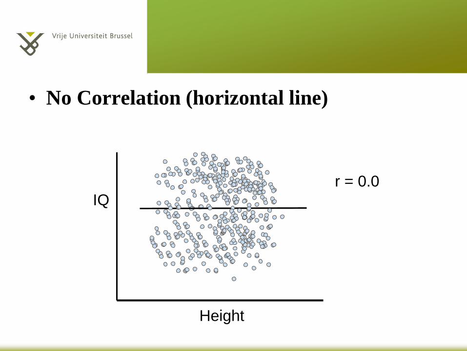
• No Correlation (horizontal line)
Height
IQ
r = 0.0
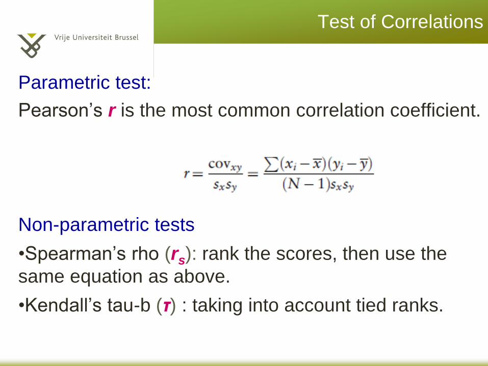
Test of Correlations
Parametric test:
Pearson’s r is the most common correlation coefficient.
Non-parametric tests
•Spearman’s rho (rs): rank the scores, then use the
same equation as above.
•Kendall’s tau-b (τ) : taking into account tied ranks.

PRACTICE
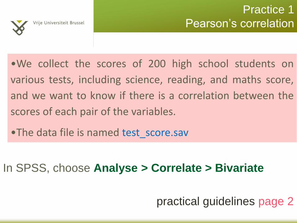
Practice 1
Pearson’s correlation
•We collect the scores of 200 high school students on
various tests, including science, reading, and maths score,
and we want to know if there is a correlation between the
scores of each pair of the variables.
•The data file is named test_score.sav
In SPSS, choose Analyse > Correlate > Bivariate
practical guidelines page 2
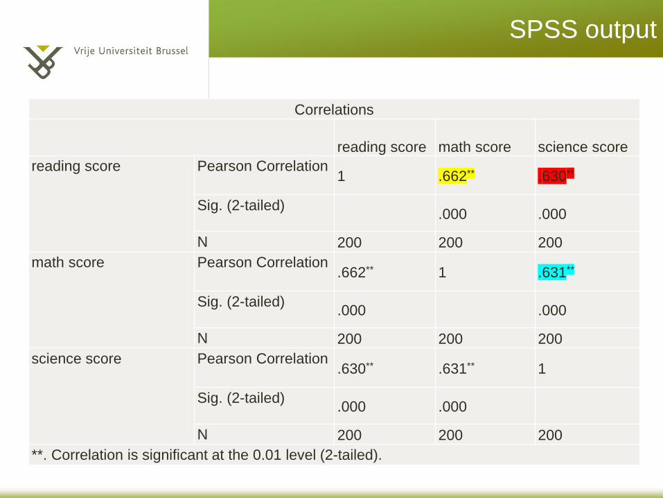
SPSS output
Correlations
reading score math score science score
reading score Pearson Correlation 1 .662** .630**
Sig. (2-tailed) .000 .000
N 200 200 200
math score Pearson Correlation .662** 1 .631**
Sig. (2-tailed) .000 .000
N 200 200 200
science score Pearson Correlation .630** .631** 1
Sig. (2-tailed) .000 .000
N 200 200 200
**. Correlation is significant at the 0.01 level (2-tailed).
Practice 1
Conclusion?
Reading scores were significantly correlated with math
scores, r = .66, p < .01 (two-tailed), and science scores, r =
.63, p < .01 (one-tailed); the math scores were also correlated
with the science scores, r = .63, p < .01 (two-tailed).
(Practical guidelines page 4)
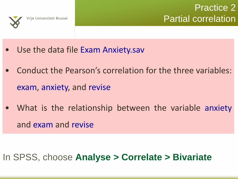
Practice 2
Partial correlation
• Use the data file Exam Anxiety.sav
• Conduct the Pearson’s correlation for the three variables:
exam, anxiety, and revise
• What is the relationship between the variable anxiety
and exam and revise
In SPSS, choose Analyse > Correlate > Bivariate
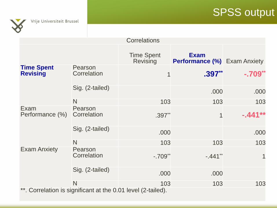
SPSS output
Correlations
Time Spent
Revising Exam
Performance (%) Exam Anxiety Time Spent Revising
Pearson Correlation 1 .397** -.709**
Sig. (2-tailed) .000 .000
N 103 103 103 Exam Performance (%)
Pearson Correlation .397** 1 -.441**
Sig. (2-tailed) .000 .000
N 103 103 103 Exam Anxiety Pearson
Correlation -.709** -.441** 1
Sig. (2-tailed) .000 .000
N 103 103 103 **. Correlation is significant at the 0.01 level (2-tailed).
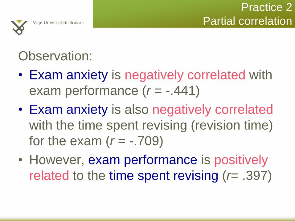
Practice 2
Partial correlation
Observation:
• Exam anxiety is negatively correlated with
exam performance (r = -.441)
• Exam anxiety is also negatively correlated
with the time spent revising (revision time)
for the exam (r = -.709)
• However, exam performance is positively
related to the time spent revising (r= .397)
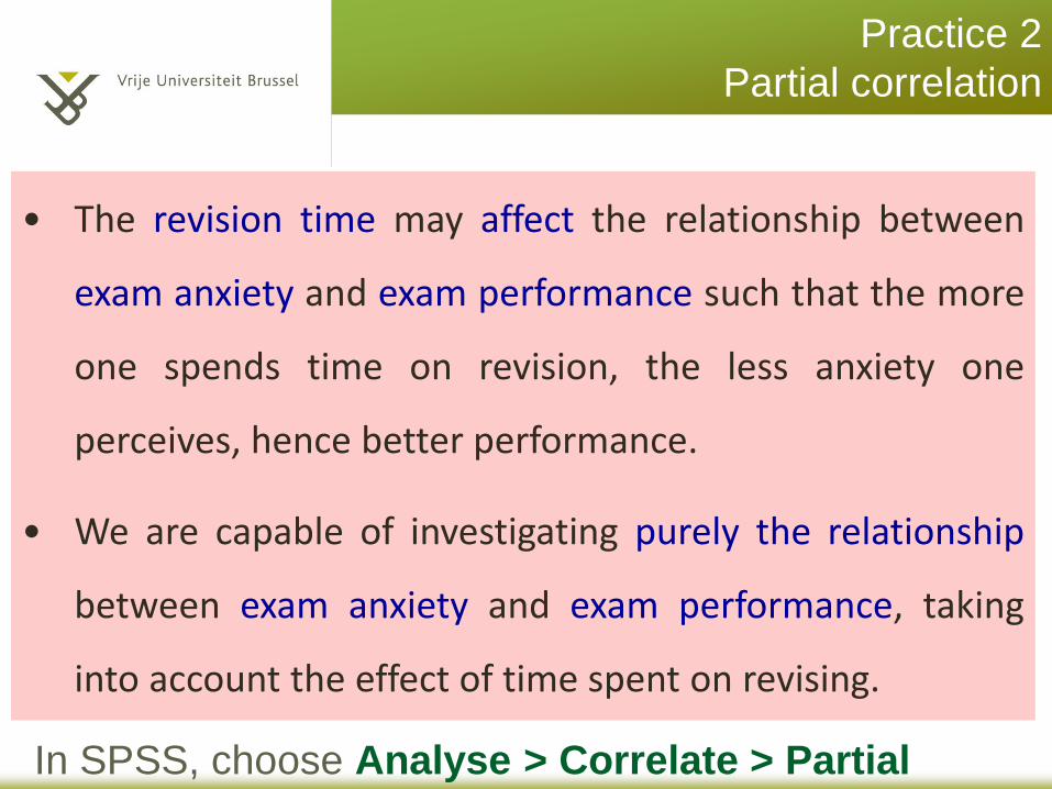
Practice 2
Partial correlation
• The revision time may affect the relationship between
exam anxiety and exam performance such that the more
one spends time on revision, the less anxiety one
perceives, hence better performance.
• We are capable of investigating purely the relationship
between exam anxiety and exam performance, taking
into account the effect of time spent on revising.
In SPSS, choose Analyse > Correlate > Partial
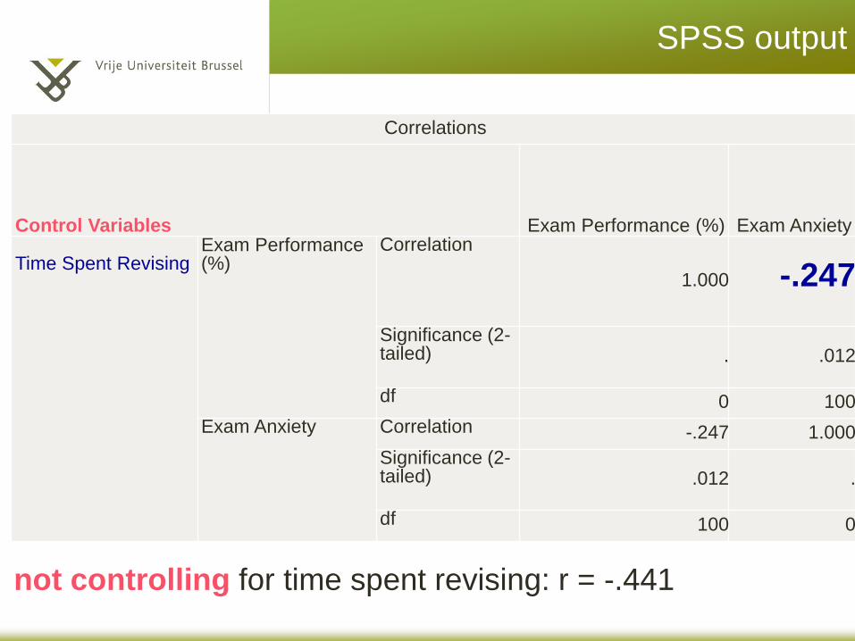
SPSS output
Correlations
Control Variables Exam Performance (%) Exam Anxiety Time Spent Revising
Exam Performance (%)
Correlation
1.000 -.247
Significance (2-tailed) . .012
df 0 100
Exam Anxiety Correlation -.247 1.000
Significance (2-tailed) .012 .
df 100 0
not controlling for time spent revising: r = -.441
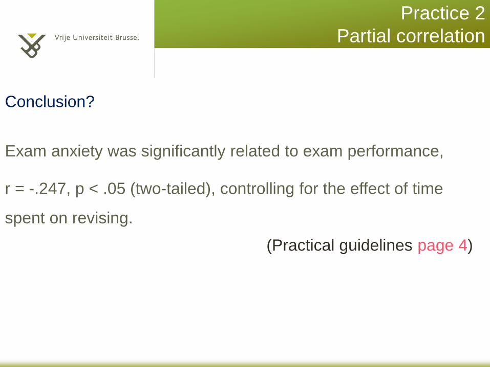
Practice 2
Partial correlation
Conclusion?
Exam anxiety was significantly related to exam performance,
r = -.247, p < .05 (two-tailed), controlling for the effect of time
spent on revising.
(Practical guidelines page 4)
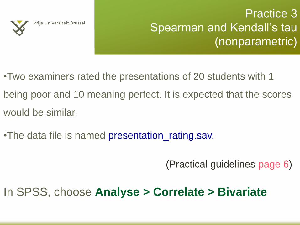
Practice 1
•Two examiners rated the presentations of 20 students with 1
being poor and 10 meaning perfect. It is expected that the scores
would be similar.
•The data file is named presentation_rating.sav.
(Practical guidelines page 6)
Practice 3
Spearman and Kendall’s tau
(nonparametric)
In SPSS, choose Analyse > Correlate > Bivariate
Practice 3
Spearman and Kendall’s tau
(nonparametric)
Conclusion?
•The rating of the two examiners was significantly correlated, rs =
.825, p < .01 (two-tailed). Or:
•The rating of the two examiners was significantly correlated, τ =
.707, p < .01 (two-tailed)
(Practical guidelines page 6)
Assignment 4
• Detail:
Lecture 4_practical guidelines_assignment
(p. 7)
Deadline: November 5, 2014