SPATIAL REGRESSION MODELS FOR YIELD MONITOR DATA: A CASE STUDY FROM ARGENTINA

Dayton M. Lambert

James Lowenberg-DeBoer

Department of Agricultural Economics/Site-Specific Management Center Purdue University 403 W State Street

West Lafayette, Indiana 47097-2056

Tel: 970-494-5818 Fax: (765) 494-9176

lambertd@purdue.edu lowenbej@purdue.edu

Rodolfo Bongiovanni National Institute for Agricultural Technology (INTA)

Ruta 9 km 636 5988 Manfredi, Argentina

Tel: (54) 3572-493039 rodolfo_bongiovanni@yahoo.com

(INTA)

Paper prepared for presentation at the American Agricultural Economics Association Annual Meeting, Montreal, Canada, July 27-30, 2003

Copyright 2003 by Dayton Lambert, James Lowenberg-DeBoer, and Rodolfo Bongiovanni. All rights reserved. Readers may make verbatim copies of this document for non-commercial purposes by any means, provided that this copyright notice appears on all such copies.

1

ABSTRACT

Precision agricultural technology promises to move crop production closer to a

manufacturing paradigm, but analysis of yield monitor, sensor and other spatial data has proven

difficult because correlation among neighboring observations often violates the assumptions of

classical statistical analysis. When spatial structure is ignored variance estimates tend to be

inflated and significance levels of test statistics are reduced. The gap between data analysis and

site-specific recommendations has been identified as one of the key constraints on widespread

adoption of precision agriculture technology. This paper compares four approaches that

explicitly incorporate spatial correlation into regression models: (1) a spatial econometric

approach; (2) a polynomial trend regression approach; (3) a classical nearest neighbor analysis;

and (4) and a geostatistic approach. In the Argentine data studied, the spatial econometric,

geostatistical approach and spatial trend analysis offered stronger statistical evidence of spatial

heterogeniety of nitrogen response than the ordinary least squares or nearest neighbor analysis.

All the spatial models led to the same economic conclusion, which is that variable rate nitrogen

is potentially profitable. The spatial econometric analysis can be implemented on relatively small

data sets that do not have enough observations for estimation of the semivariogram required by

geostatistics. The spatial trend analysis can be implemented with ordinary least squares functions

that are already available in some GIS software. In this study, the main benefit of using spatial

regression analysis is increased confidence in the corn yield response estimates by management

zone, and conclusions about the profitability of precision agriculture technologies.

Keywords: Spatial econometrics, precision agriculture, regression, nearest neighbor, polynomial trend, geostatistics

2

INTRODUCTION Precision agriculture technology is moving farming in the direction of “production to

specification” that has long characterized manufacturing. In their textbook on production and

operations management for manufacturing, Chase et al. (1998) cite precision agriculture as one

of the most dramatic examples of technological change within an industry, but adoption of this

technology has been relatively slow. One of the key barriers has been analysis of spatial crop

and livestock data (Bullock et al., 2002). The gap between data analysis and site-specific

recommendations makes it difficult to determine how seed, pesticide, fertilizer and other inputs

should be varied to maximize profits, minimize environmental impacts and achieve other goals.

Classical statistics applied to agronomic plots and to on-farm experiments assume that

observations are independent, but in the case of precision agriculture data this assumption of

independence is untenable. Any yield monitor observation is clearly correlated to its neighboring

observations. Spatial statistics with differing models of correlation among neighboring

observations have been developed in a variety of contexts (e.g. geography, regional economics,

geology). The general objective of this study was to determine which spatial regression model

leads to the best economic decisions. A case study of maize response to nitrogen in central

Argentina is examined.

Precision agriculture has captured the imagination of producers and agribusiness, but

adoption has been relatively slow. For the 2001 harvest about 34% of U.S. corn area was

harvested with a combine equipped with a yield monitor (Daberkow et al., 2002), but only about

one third of those combines were equipped with a GPS that would allow them to make yield

maps. Only about 11% of corn, 6% of soybean and 4% of cotton area was managed with variable

rate fertilizer applications in 2000. Variable rate seeding and pesticide application was used on

3

1% to 3% of area depending on the crop. Bullock et al. (2002) identify the lack of site-specific

crop response information as a key constraint to adoption of spatial crop management. Most

variable rate input application is still based on whole field crop response information. They argue

that if producers could more easily gather and analyze the crop responses for their specific soils,

micro-climate and management, then precision agriculture would be more profitable and the

social goals of using this technology to improve environmental performance and food safety

could be more easily achieved.

Most of the whole field crop response information has been analyzed with ordinary least

square regression and similar statistical tools. But precision of yield response functions based on

OLS estimates can be compromised by spatially autocorrelated data (Kessler and Lowenberg-

DeBoer, 1998). Consequently, field heterogeneity may be underestimated, and inferences about

crop response to variable fertilizer rates may be inefficient or biased. Incorrect inference may

lead to inaccurate profitability analysis of trials comparing variable rate application of nitrogen

(VRN) to conventional, uniform fertilization rates (Bongiovanni and Lowenberg-DeBoer, 2000;

Lambert et al., 2002). In general, when field heterogeneity is ignored variable rate technology

profit margins may appear less reliable. A key step in making precision farming both more

profitable and practical is the development of consistent and reliable estimation procedures that

account for spatially correlated data.

This paper compares corn response to variable rate nitrogen (VRN) applications

estimated by five regression techniques: (i) ordinary least squares (OLS); (ii) a restricted

maximum likelihood (REML) geostatistics approach (Cressie, 1993; Schabenberger and Pierce,

2002); (iii) a spatial econometric approach (Anselin, 1988); (iv) a polynomial trend analysis

approach (Tamura et al., 1988); and (v) a classical nearest neighbor approach first suggested by

4

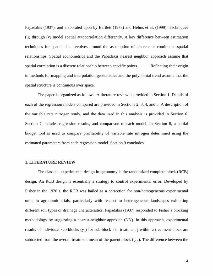
Papadakis (1937), and elaborated upon by Bartlett (1978) and Helms et al. (1999). Techniques

(ii) through (v) model spatial autocorrelation differently. A key difference between estimation

techniques for spatial data revolves around the assumption of discrete or continuous spatial

relationships. Spatial econometrics and the Papadakis nearest neighbor approach assume that

spatial correlation is a discrete relationship between specific points. Reflecting their origin

in methods for mapping and interpolation geostatistics and the polynomial trend assume that the

spatial structure is continuous over space.

The paper is organized as follows. A literature review is provided in Section 1. Details of

each of the regression models compared are provided in Sections 2, 3, 4, and 5. A description of

the variable rate nitrogen study, and the data used in this analysis is provided in Section 6.

Section 7 includes regression results, and comparison of each model. In Section 8, a partial

budget tool is used to compare profitability of variable rate nitrogen determined using the

estimated parameters from each regression model. Section 9 concludes.

1. LITERATURE REVIEW

The classical experimental design in agronomy is the randomized complete block (RCB)

design. An RCB design is essentially a strategy to control experimental error. Developed by

Fisher in the 1920’s, the RCB was hailed as a correction for non-homogeneous experimental

units in agronomic trials, particularly with respect to heterogeneous landscapes exhibiting

different soil types or drainage characteristics. Papadakis (1937) responded to Fisher’s blocking

methodology by suggesting a nearest-neighbor approach (NN). In this approach, experimental

results of individual sub-blocks (yij) for sub-block i in treatment j within a treatment block are

subtracted from the overall treatment mean of the parent block ( jy ). The difference between the

5

sub- and whole-block values is the experimental error for yij. In the classical NN analysis,

neighbors are arranged perpendicularly: every observation has four neighbors. Thus the error of

yij is the average of the error terms of its four neighbors sharing the same boundary. Observations

located on the edge of the experimental plot are weighted accordingly.

Bartlett (1978) brought to fore Papadakis’ nearest neighbor approach for field trials.

Nearest neighbor approaches have been compared to standard blocking methods by Stroup et al.

(1994). Using a lattice experimental design, Vollman et al. (2000) used the classic Papadakis NN

approach to identify spatial trend patterns between experimental plots for soybean. They found

that soybean yield, seed protein quantity, and seed size were affected by spatial heterogeneity

between plots. An iterative NN approach (Schwarzbach, 1984) was used by Helms et al. (1995,

1999) to compare block by treatment and pooled error means for comparing soybean variety

performance using ANOVA. They found little difference between classical blocking and NN

techniques in regards to reducing error caused by within-block spatial heterogeneity. Precision of

between-plot variance estimates (pure error) was similar for NN and classical experimental

designs.

Tamura et al. (1988) provide another alternative to Fisher’s blocking scheme by inserting

a polynomial trend variable (Tij) into the familiar ANOVA model Yij� �� �� �� �ij �� �ij. This

approach is related to the spatial expansion regression methodology that has received attention in

urban and regional geography (Anselin, 1988). A trend surface is introduced into the model

specification to simulate spatial relations between observations. This approach assumes that

omission of spatial dependencies is analogous to the omitted variable problems in econometrics.

The omitted variable problem is by-passed by inclusion of trend variables in ANOVA models.

Like the NN method proposed by Papadakis, Tamura et al.’s (1988) polynomial trend (PTR)

6

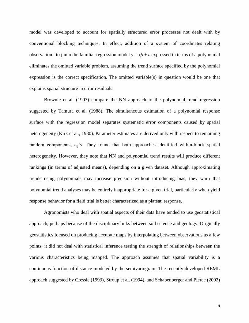
model was developed to account for spatially structured error processes not dealt with by

conventional blocking techniques. In effect, addition of a system of coordinates relating

observation i to j into the familiar regression model y = �� + � expressed in terms of a polynomial

eliminates the omitted variable problem, assuming the trend surface specified by the polynomial

expression is the correct specification. The omitted variable(s) in question would be one that

explains spatial structure in error residuals.

Brownie et al. (1993) compare the NN approach to the polynomial trend regression

suggested by Tamura et al. (1988). The simultaneous estimation of a polynomial response

surface with the regression model separates systematic error components caused by spatial

heterogeneity (Kirk et al., 1980). Parameter estimates are derived only with respect to remaining

����� ��� ����� �ij’s. They found that both approaches identified within-block spatial

heterogeneity. However, they note that NN and polynomial trend results will produce different

rankings (in terms of adjusted means), depending on a given dataset. Although approximating

trends using polynomials may increase precision without introducing bias, they warn that

polynomial trend analyses may be entirely inappropriate for a given trial, particularly when yield

response behavior for a field trial is better characterized as a plateau response.

Agronomists who deal with spatial aspects of their data have tended to use geostatistical

approach, perhaps because of the disciplinary links between soil science and geology. Originally

geostatistics focused on producing accurate maps by interpolating between observations as a few

points; it did not deal with statistical inference testing the strength of relationships between the

various characteristics being mapped. The approach assumes that spatial variability is a

continuous function of distance modeled by the semivariogram. The recently developed REML

approach suggested by Cressie (1993), Stroup et al. (1994), and Schabenberger and Pierce (2002)

7

includes estimating empirical semivariograms, and then using these parameter estimates as priors

in a regression model to identify spatial error covariance structures.

Lambert et al. (2002) used the REML-geostatistics approach suggested by Cressie (1993)

and explicitly detailed by Schabenberger and Pierce (2002) to analyze yield monitor data.

Parameter estimates of corn response to nitrogen and resulting profitability estimates of VRN

technology were similar to estimates produced using the spatial econometric approach. A similar

approach combining geostatistics was taken by Hurley et al. (2001). They estimated the

profitability of soil tests, topographical, and remote sensing information for corn with a three

step regression using semivariogram priors incorporating spatial error process into regression

variance-covariance (VC) matrices.

Spatial econometric techniques have been extended to analysis of crop yield data in

general, and yield monitor data in particular. Bongiovanni and Lowenberg-DeBoer (2001, 2002)

adapted the spatial econometric approach to analyze profitability of VRN applications to corn

using yield monitor data. They found that econometric spatial autoregressive (SAR) estimates

were more precise than OLS estimates since the SAR model corrects for spatial structure in the

error terms. With the SAR model, standard error estimates of corn response to nitrogen

parameters are no longer inefficient, and therefore produced more precise estimates. From an

economic perspective, better estimates translated into a more accurate account of VRT

profitability. In these studies, more reliable estimates of VRT profitability were developed when

spatial autocorrelation was taken into consideration.

2. ECONOMETRIC APPROACH TO SPATIAL REGRESSION

8

The spatial econometric approach (Anselin, 1988) assumes that spatial variability is a

relationship among discrete observations. Spatial structure may be found in either the dependent

variable (e.g. yield) or in error residuals terms. Spatial structure is modeled assuming that the

dependent variable or residuals are a function of a weighted sum of neighboring data. This

discrete approach has been used extensively in epidemiology, criminology and regional

economics. In agriculture the structure of the data is similar, but the polygons are often soil types

or management zones instead of states, counties, districts, or neighborhoods. The discrete

approach enables simultaneous maximum likelihood estimation of the spatial structure and the

relationships between GIS layers. Effects of temporal correlation and heteroskedasticity can be

incorporated.

Spatially autocorrelated data, or spatial dependence, is the special case where the

dependent variable or error term at each location is correlated with observations of the dependent

variable or error terms at other locations (Anselin, 1992). To test for spatial effects in

econometric models, spatial weights matrices are constructed and then included in a specified

regression model. Spatial matrices are designed to incorporate processes such as gravity,

entropy, or decay into autocorrelated regression models (Anselin, 1988). Data arranged in

regular rectangular lattices are defined using three criterions: bishop, rook, or queen. These

classes describe the level of contiguity, or common boundaries, between polygons. The

econometric regression in this study used the queen criterion: individual grids have both a border

and a corner in common with one or more other grids. In spatial terms, contiguity is defined as a

function of the distance that separates one grid from another. Blocks belonging to the same

neighborhood share the same weight, and the composite of neighborhoods covering the entire

grid defines the spatial weights matrix. This matrix is an N x N, positive definite matrix with

9

elements wij. Before spatial weights matrices are used to estimate spatial effects in regression

models, they are row-standardized. This facilitates comparison of spatial characteristics across

neighborhoods. Each element in a row is divided by the row sum. Individual elements in a row-

standardized matrix take the form ∑=j ijijij www where 1=Σ ijj w .

In general, there are two patterns whereby spatial dependence may manifest itself in

regression analysis: spatial lag and spatial error. If spatial error processes are ignored, OLS

estimates become inefficient, but remain unbiased. If spatial lag processes are ignored, then OLS

estimates are inconsistent and biased. The presence of these effects are only determined when a

regression model is estimated with OLS concomitantly with its associated spatial matrix.

Observations in the spatial matrix are identified with observations in the corresponding data set

used to estimate parameters. By incorporating the problem’s spatial weight matrix W into the

regression model, relations between the dependent variable yi with neighboring yi’s or error

terms are determined for lag and error classifications, respectively. For lag processes, the

modified regression model y = �� + � becomes:

y ���Wy +��� + � (1)

with � being the autoregressive moving average parameter for neighboring yi’s. The spatial error

model is specified as:

y = �� + � (2)

�������� + � (3)

The specified error term is represented by ��, while � represents well-behaved, non-

heteroskedastic, uncorrelated errors. Rho can be estimated with maximum likelihood (ML) or

with two-���� �� ��������� ���� � ������������ ����� ���������� ������������

10

Spatial ������� �������� �� � ������������������ ��������2(1) variate; Anselin, 1988) test

for the presence of spatial dependence. The alternative hypothesis of the LMerror test is that

residuals follow a spatial pattern, while the alternative hypothesis of the LMlag test is that

individual observations on explanatory and/or the dependant variables are correlated with the

average of other values of the same variables in a given neighborhood of observations. To

correct for possible asymptotic interdependence between LM error and lag tests, the LMerror and

LMlag robust tests filter out correlation that might be due to covariance between autoregressive

lag and autoregressive or moving average error terms. Rejection of the null hypothesis for the

LMlag test means that the researcher faces an omitted variable problem; OLS estimates are biased

and inconsistent. If the null hypothesis of the LMerror test is rejected, the researcher faces an

efficiency problem; OLS estimates are not biased, but they are inefficient. Hence, t-tests and

standard errors are biased, and inference about parameters is compromised.

3. GEOSTATISTIC APPROACH TO SPATIAL REGRESSION

Schabenberger and Pierce (2002) define the geostatistic method of estimating regression

parameters as entailing modeling at two levels: the mean function (first-order properties) of the

process and concomitant spatial dependency structures (second-order properties). Modeling of

the second-order properties involves fitting a semivariogram to an empirical semivariogram of

the spatial process or the raw data to produce parametric estimates. In general, geostatistics

emphasizes prediction of attributes at a particular location. It is assumed that the spatial process

follows a gaussian distribution in the limit. Additionally, it is assumed the mean response

function is linear. This approach explicitly handles spatially autocorrelated error terms.

The geostatistics spatial model is given by:

11

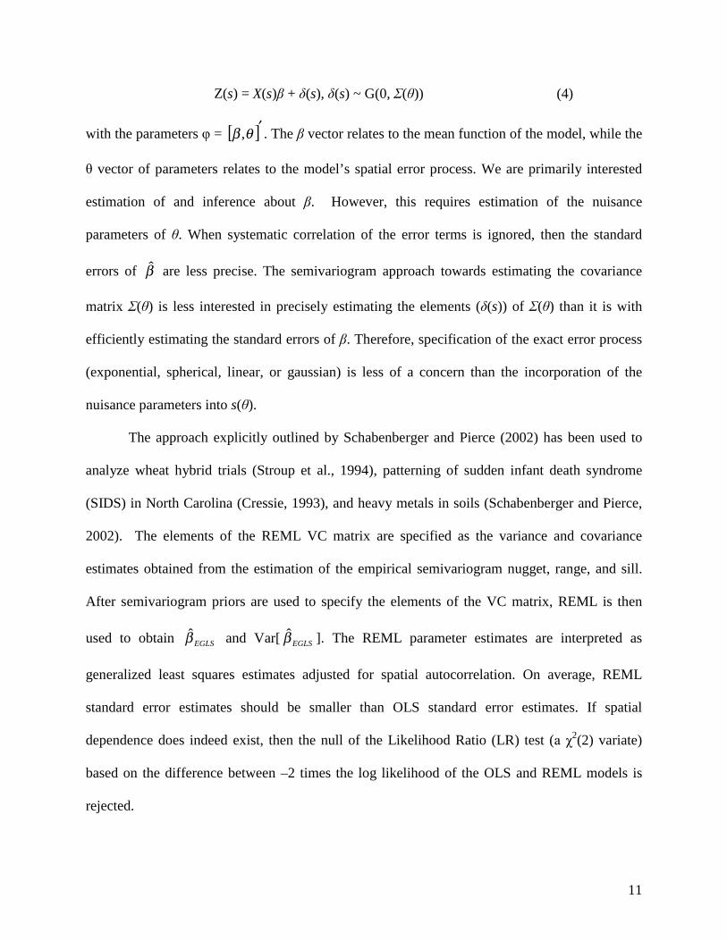
Z(s) = X(s)� + �(s), �(s) ~ G(0, �(�)) (4)

with the parameters � = [ ]′θβ , . The � vector relates to the mean function of the model, while the

� vector of parameters relates to the model’s spatial error process. We are primarily interested

estimation of and inference about �. However, this requires estimation of the nuisance

parameters of �. When systematic correlation of the error terms is ignored, then the standard

errors of β are less precise. The semivariogram approach towards estimating the covariance

matrix �(�) is less interested in precisely estimating the elements (�(s)) of �(�) than it is with

efficiently estimating the standard errors of �. Therefore, specification of the exact error process

(exponential, spherical, linear, or gaussian) is less of a concern than the incorporation of the

nuisance parameters into s(�).

The approach explicitly outlined by Schabenberger and Pierce (2002) has been used to

analyze wheat hybrid trials (Stroup et al., 1994), patterning of sudden infant death syndrome

(SIDS) in North Carolina (Cressie, 1993), and heavy metals in soils (Schabenberger and Pierce,

2002). The elements of the REML VC matrix are specified as the variance and covariance

estimates obtained from the estimation of the empirical semivariogram nugget, range, and sill.

After semivariogram priors are used to specify the elements of the VC matrix, REML is then

used to obtain EGLSβ and Var[ EGLSβ ]. The REML parameter estimates are interpreted as

generalized least squares estimates adjusted for spatial autocorrelation. On average, REML

standard error estimates should be smaller than OLS standard error estimates. If spatial

dependence does indeed exist, then the null of the Likelihood Ratio (LR) test (���2(2) variate)

based on the difference between –2 times the log likelihood of the OLS and REML models is

rejected.

12

4. NEAREST NEIGHBOR APPROACH AND SPATIAL REGRESSION

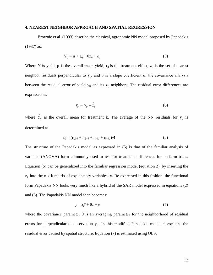
Brownie et al. (1993) describe the classical, agronomic NN model proposed by Papadakis

(1937) as:

Yij��������ij�����ij����ij (5)

�� � � ������ ������ ��� �� �! ����� ����� �����ij is the treatment effect, zij is the set of nearest

neighbor residuals perpendicular to yij�� ������ ��� �� ��� � � ""��� ��� "� �� � �!������ � ���������

between the residual error of yield yij and its zij neighbors. The residual error differences are

expressed as:

kijij Yyr ˆ−= (6)

where kY is the overall mean for treatment k. The average of the NN residuals for yij is

determined as:

zij = (ri,j-1 + ri,j+1 + ri-1,j + ri+1,j)/4 (5)

The structure of the Papadakis model as expressed in (5) is that of the familiar analysis of

variance (ANOVA) form commonly used to test for treatment differences for on-farm trials.

Equation (5) can be generalized into the familiar regression model (equation 2), by inserting the

zij into the n x k matrix of explanatory variables, x. Re-expressed in this fashion, the functional

form Papadakis NN looks very much like a hybrid of the SAR model expressed in equations (2)

and (3). The Papadakis NN model then becomes:

y = ������z + � (7)

#� � � �� � �!������ � ���� � �� �� ��� ��� �! ������� ���� � �� "�� �� � � �������� "� � �������

errors for perpendicular to observation yij�� $�� ����� ��"� �� %�����&��� � ��� �� '������� �� �

residual error caused by spatial structure. Equation (7) is estimated using OLS.

13

5. POLYNOMIAL TREND REGRESSION AND SPATIAL REGRESSION

The PTR model is specified as (Tamura et al., 1988; Brownie et al., 1993):

Yij��������k(ij) + Tij����ij (8)

with Y ����� ��� ����������� �! ����� �����k������ ��� �� ��� "" ��������������������� ����������

is an i.i.d. random error component. The polynomial trend term is estimated as:

Tij���1'����2�����3x2����4y

2����5xy (9)

#� � ��i is a slope coefficient for the Cartesian (x,y) coordinate of observation yij. The model

suggested by Tamura et al. (1988) can be re-written as and then estimated with the familiar

regression equation of (2). The (x,y) coordinates, their squares, and their interaction are placed in

the x matrix of explanatory variables in (2), and the model is estimated using OLS.

6. DATA

Corn nitrogen response data from the study by Bongiovanni and Lowenberg-DeBoer

(2001) was used. The data were collected from strip trials at the “Las Rosas” farm located in the

Río Cuarto area, Córdoba Province, Argentina, in the 1998-99 crop season. The strips were the

width of the N applicator (9.8 m), with a zero N control and five other rates of elemental N: 29,

53, 66, 106, and 131.5 kg ha-1. The N rate was constant for the whole strip, across the four

topographies identified. The highest N rate for each field was higher than the expected yield

maximizing level. The N source was urea. Data was collected with a standard AgLeaderTM

yield monitor. Since the raw data includes data points that are closer within the same row than

between rows, these data yield points were averaged for a within-row distance equivalent to the

between-rows distance, such that a distance weights matrix could be calculated for ML

estimation of lag and error processes. This was done in the GIS software SSToolboxTM, creating

14

9.8 x 9.8 meter grids over the observations, and rotating them by 10.5 degrees. Data points at the

extreme left and at the extreme right were deleted, because they reflect an empty combine

entering the row. Finally, and after averaging the data within each grid, the 1738 grids

(observations) were digitized as polygons. Centroid points generated by ArcViewTM of each grid

were used to estimate empirical semivariograms.

The base regression model is quadratic in form:

Y = �o + �1N + �2N2 + �i + interaction terms + � (9)

where:

Y = corn yield (t/ha);

N = kilograms of elemental nitrogen fertilizer per ha;

�i = a dummy variable specified as 04

=∑=

n

iiδ indicating topographical variability (TOP1

= lowland, TOP2 = east slope, TOP3 = hilltop, TOP4 = west slope);

� is an i.i.d. error term ~ N(0, I�2).

Topographical zones were delineated by INTA agronomists as areas with common landscape

attributes (e.g. slope, aspect, soil color).

7. RESULTS

Geostatistic-REML approach

Restricted estimated maximum likelihood estimates using gaussian and exponential

semivariogram priors are reported in Lambert et al. (2002). In this study, REML results using

spherical and linear response plateau (LRP) semivariogram priors are reported since both

15

specifications out-performed the gaussian and exponential functional forms in terms of overall fit

(R2) and F-test scores. Non-linear weighted least squares estimates for the LRP and spherical

models were significant at P < 0.01, as well as F-values for each model. The nugget effect

(“white noise”) for the LRP semivariogram model (9.71) is larger than that of the spherical

model (9.00, Figure 1). The range parameter for the spherical model was 140 m, while the range

of the LRP was 112 m. Sill values for the spherical and LRP models were ���(� �� )*�+,� ����

35.48, respectively. The LRP model best fit the data (R2 = 0.98), while the coefficient of

determination for the spherical model was 0.70. The F-test values for the spherical and LRP

semivariogram models were 605 and 2793, respectively. The error explained spatially by the

semivariograms is determined as (sill/[sill + nugget effect]). The percent of spatial heterogeneity

explained by the LRP and spherical models were nearly identical (79 and 80%, respectively).

Spherical and LRP REML model fit statistics are presented in Table 1. Likelihood ratio

tests were strongly significant for both models (P<0.0001), indicating that the model error

disturbances are correlated and not equally distributed in the data set. According to the log

likelihood criterion, the LRP model had the best fit compared to the spherical REML model

within this class of regression models. This is expected since the fit of the empirical

semivariogram by the LRP form was more precise compared to the spherical model. Information

produced in the fitting process of the empirical semivariogram gives a reasonable criterion upon

which to base the specification of the REML VC matrix in the regression estimation step.

Estimated generalized least squares parameter estimates adjusted for spatial dependence are

presented in Table 2.

The LRP and spherical REML models produced the same number of significant

parameter estimates. However, rejection of the T-test null hypotheses for parameter significance

16

of the LRP model was generally stronger than those of the spherical model. That the REML

regression results using the LRP semivariogram priors produced more precise results than the

REML model using spherical priors is expected given the excellent fit of the empirical

semivariogram by the LRP specification.

Spatial econometric approach

�� ���� � ��� "�� �������� ������ ������#��� ������� �����"������ "�� ���� ��(� ���� ���� ��(�

parameters when the spatial weights matrix was included in the OLS regression (LM = 514 and

705, respectively). However, the robust LM test for spatial error process was highly significant

(LM = 195, P<0.0001), whereas the LM robust score for spatial lag autocorrelation was not (LM

= 3.21, P = 0.07). Based on this criterion, the null that there is no spatial structure in the

regression errors is rejected. The best specification is the spatial error model (SAR). Model fit

statistics are presented in Table 1.

The null hypothesis of no spatial dependence was also strongly rejected by the LR for the

SAR model (1231, respectively, df = 2, P < 0.0001). Parameter estimates for SAR ML model are

presented in Table 2. The Z-��� ��������� ��#������ ����� �� ���! �������� ����� � ����# � �

highly significant (P < 0.0001), indicating the presence of spatial structure in the residual error

terms.

Nearest neighbor approach

The NN model improved the coefficient of determination by 6%, compared to the OLS-

based estimates (Adjusted R2 = 0.60, Table 1). This is expected because of the addition of the

�!������ ����� � ������-# ! �������his case the appropriate measure of fit statistic is the AIC

17

criterion since an additional parameter was included in the regression model. The NN regression

improved the AIC criterion by only 2.5%. However, the LR test for spatial dependence was

significant (LR = 282, df = 2, P < 0.0001), indicating the presence of spatial structure in the

model error terms. Presence of spatial dependence is also indicated by the P-value (P < 0.0001)

"���� ��!������ ����� � �����

Polynomial trend regression

The null hypothesis of no spatial structure in the regression error terms was strongly

rejected when the model was estimated using the PTR specification (LR = 984, df =2, P <

0.0001, Table 1). Compared to the original OLS model fit, the Adjusted R2 for the PTR increased

by 18%. However, because (x,y) coordinates for each observation in the data set were increased

the number of regressors by five, the appropriate fit statistic is the AIC criterion. Following the

AIC criterion, the PTR model improved the overall fit of the data by 9%.

Comparison of spatial regression models

The base OLS model AIC fit criterion was improved between 3% and 15% when error

spatial dependence was included in the model. All models produced the expected signs for the

quadratic yield response to nitrogen, and all topography intercept terms were significant in each

of the models. The frequency of significant parameter estimates increased with all models that

accounted for spatial heterogeneity. When heteroskedasticity between topographical zones was

not taken into consideration, the fit of REML-LRP and SAR ML models is very similar.

In general, the slope coefficients for all spatial regression models are very similar. The

major differences between the results were the intercept terms for each topographical region, and

18

the magnitude of parameter significance. On average, the standard errors of the SAR ML model

were 17% less than the OLS model (excluding the constant standard error). Standard errors of

the REML regressions using LRP and spherical semivariogram priors were on average 3%

(spherical) to 16% (LRP) smaller than the OLS standard error estimates. The difference in

magnitude between the REML-LRP and REML spherical specification relates to the differences

of fit of the empirical semivariogram by LRP and spherical functional forms. Estimated standard

errors of the PTR and NN regression models were smaller than the OLS base model by 3% and

7%, respectively. As a result of the smaller standard error, SAR models have more significant

coefficients than the OLS, PTR, NN, and the REML spherical models. However, there is little

difference between SAR ML and REML-LRP results. In terms of interpretation, NN results are

similar to OLS estimates. The AIC does not decrease substantially with the NN model, and only

one nitrogen by topography interaction is significant. The PTR approach does surprisingly well

for a simple approach that could be implemented with very simple regression software. Like the

REML approaches, the PTR has two significant nitrogen by topography interaction terms.

8. NITROGEN BUDGETING AND VRT PROFITABILITY USING REGRESSION

ESTIMATES

Accounting for spatial dependency in yield monitor data has a significant effect on the

inferences drawn about VRT profitability (Table 3). Returns from N above fertilizer cost were

estimated for a uniform application rates and for VRT by landscape position. The uniform N rate

was 36.8 kg ha-1 recommended by Castillo et al. (1998). Estimated VRT applications assumed

that N varied by landscape position according to the profit maximizing levels. All estimates use

the response curves by landscape to estimate yield, which is weighted by the corresponding

19

topography areas (Low = 27%, Slope E = 21%, Hilltop = 20% and Slope W = 32%). Returns

above fertilizer cost were estimated as follows: Returns above fertilizer cost ($ ha-1)

= [ ]( )NPNNP Niiici

i −++∑=

2210

4

1

βββω where: Pc= Price of corn ($6.85 quintal-1); i =

Topography zone (1=Low E, 2= Slope E, 3=Hilltop, 4=Slope W); N = N rate (profit max N* rate

for VRT computations); PN = Price of N fertilizer ($0.435 kg-1), plus interest for 6 months at

15% annual interest rate; �i = % of landscape represented by topography zone i.

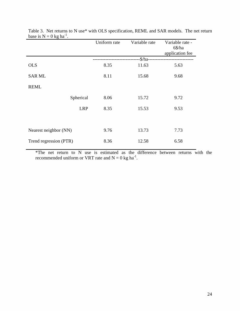
The net return to N use is $7 to $8 ha-1 greater when using the spatial regression

estimates. This would allow the producer to pay the estimated $6 ha-1 fee for custom VRT

application and retain a modest profit. As pointed out by Bongiovanni and Lowenberg-DeBoer

(2001) spatial regression results in a very different VRT decision in this case than OLS. An

analyst using REML, NN or the SAR approaches would find statistical support for significant

differences between N response by landscape area and economic evidence for VRT profitability.

An analyst using OLS would conclude that the N response is the same in all landscape areas and

that VRT is unprofitable at the estimated $6 ha-1 custom application fee.

Variances of the point estimates for returns to VRT and uniform rates were approximated

using a Taylor series expansion (Cassella and Berger, 1990). The variability of returns to VRT

was greatest when profitability was estimated using the PTR model ($40.33 ha-1, standard

deviation, including $6 ha-1 application fee, Figure 2). Variability of returns to VRT is lowest

when estimated with REML-LRP approach ($14.13 ha-1), followed by the SAR ML approach

($11.27 ha-1). The NN variability of returns to VRN was $16.69 ha-1, and only $8.96 ha-1 for

profitability estimated from OLS estimates. However, because of the Gauss-Markov violations

"��� �./'0�1���+��'���2�3� ����� ���� ������ ����4������ the performance of the models

that correct this violation, VRN profitability is less certain with the PTR since the standard error

20

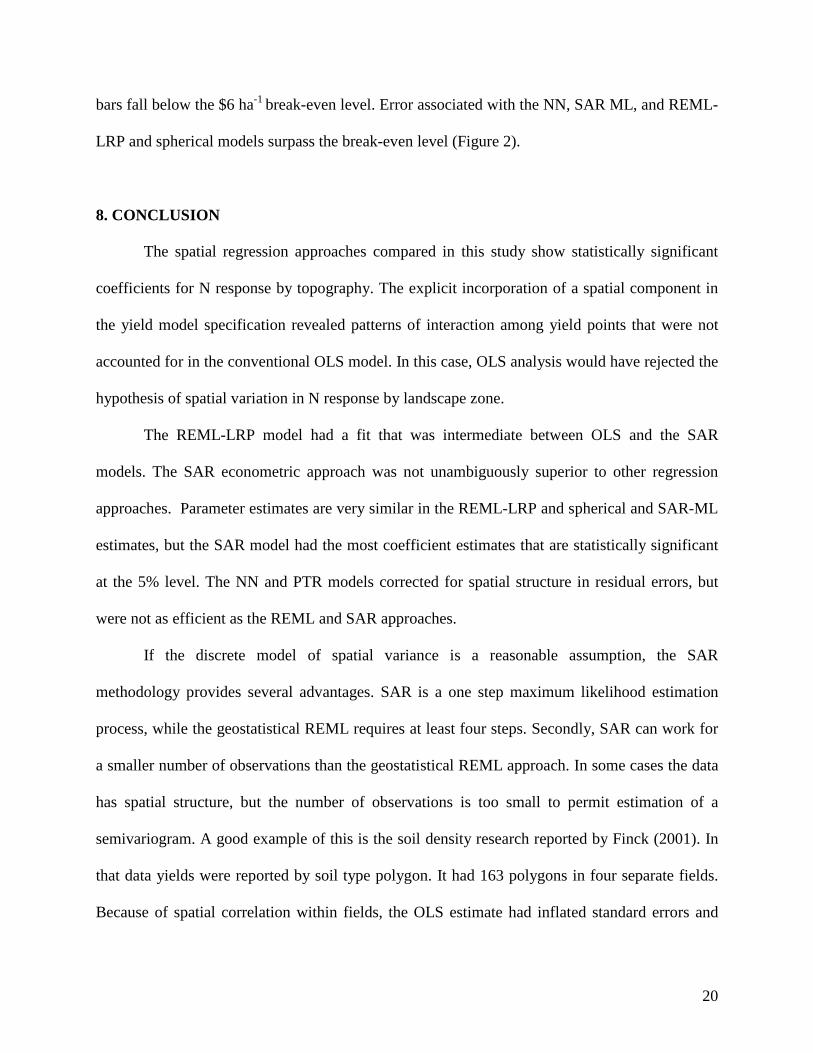
bars fall below the $6 ha-1 break-even level. Error associated with the NN, SAR ML, and REML-

LRP and spherical models surpass the break-even level (Figure 2).

8. CONCLUSION

The spatial regression approaches compared in this study show statistically significant

coefficients for N response by topography. The explicit incorporation of a spatial component in

the yield model specification revealed patterns of interaction among yield points that were not

accounted for in the conventional OLS model. In this case, OLS analysis would have rejected the

hypothesis of spatial variation in N response by landscape zone.

The REML-LRP model had a fit that was intermediate between OLS and the SAR

models. The SAR econometric approach was not unambiguously superior to other regression

approaches. Parameter estimates are very similar in the REML-LRP and spherical and SAR-ML

estimates, but the SAR model had the most coefficient estimates that are statistically significant

at the 5% level. The NN and PTR models corrected for spatial structure in residual errors, but

were not as efficient as the REML and SAR approaches.

If the discrete model of spatial variance is a reasonable assumption, the SAR

methodology provides several advantages. SAR is a one step maximum likelihood estimation

process, while the geostatistical REML requires at least four steps. Secondly, SAR can work for

a smaller number of observations than the geostatistical REML approach. In some cases the data

has spatial structure, but the number of observations is too small to permit estimation of a

semivariogram. A good example of this is the soil density research reported by Finck (2001). In

that data yields were reported by soil type polygon. It had 163 polygons in four separate fields.

Because of spatial correlation within fields, the OLS estimate had inflated standard errors and

21

few statistically significant coefficients. SAR provided a parsimonious model that allowed the

analysts to identify statistically significant effect of the soil density treatment on heavy, lowland

soils. The geostatistical REML approach suggested by Cressie (1993) and Schabenberger and

Pierce (2002) is a good alternative to SAR when: (1) Enough data is available to estimate

semivariograms, and (2) the discrete model of spatial variance structure is untenable. The

geostatistical REML approach may facilitate interdisciplinary communication. For most

economists both spatial econometrics and the geostatistical REML approach are modest

extensions of familiar regression models. Many agronomists and soil scientists are familiar with

geostatistics, but they do not regularly use regression analysis. The spatial econometrics

approach may appear very foreign to many agronomists and soil scientists, while the use of

geostatistical concepts in geostatistic REML may help create confidence. If the coefficients

estimates are similar and the geostatistical REML fit as close to that of the SAR estimates as in

the Las Rosas 99 case, the cost of using the geostatistic REML seems to be relatively small.

Another advantage of the geostatistic REML approach is that it can be implemented with the

widely available SAS software.

With increased precision available to the producer, better, more precise

statistical/regression methodologies have to be developed to take advantage of the information

these technologies provide. This brings up the issue of which statistical methodologies are most

appropriate when gauging profitability of precision technologies. It may be that because the

information provided by these new tools is so spatially dense (vertically and horizontally, or

between individual observations and GIS layers, respectively), the only appropriate and unbiased

way to properly estimate returns to these technologies is with statistical instruments that

explicitly model spatial correlation.

22

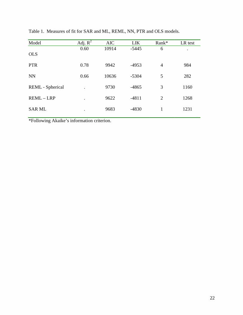
Table 1. Measures of fit for SAR and ML, REML, NN, PTR and OLS models. Model Adj. R2 AIC LIK Rank* LR test OLS

0.60 10914 -5445 6 .

PTR 0.78 9942 -4953 4 984

NN 0.66 10636 -5304 5 282

REML - Spherical . 9730 -4865 3 1160

REML – LRP . 9622 -4811 2 1268

SAR ML . 9683 -4830 1 1231

*Following Akaike’s information criterion.

23

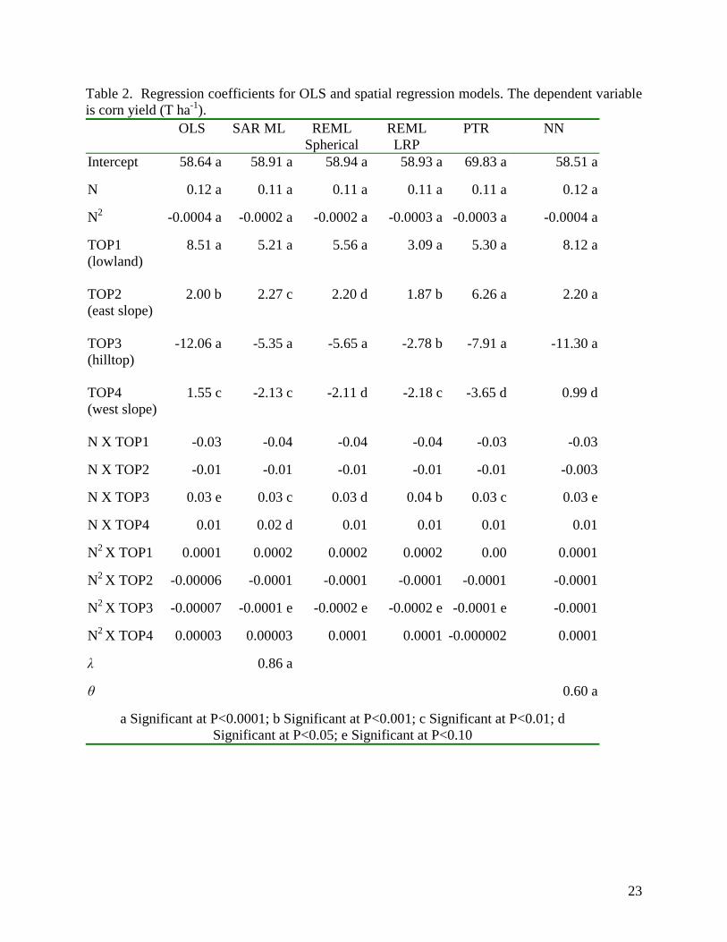
Table 2. Regression coefficients for OLS and spatial regression models. The dependent variable is corn yield (T ha-1).

OLS SAR ML REML Spherical

REML LRP

PTR NN

Intercept 58.64 a 58.91 a 58.94 a 58.93 a 69.83 a 58.51 a

N 0.12 a 0.11 a 0.11 a 0.11 a 0.11 a 0.12 a

N2 -0.0004 a -0.0002 a -0.0002 a -0.0003 a -0.0003 a -0.0004 a

TOP1 (lowland)

8.51 a 5.21 a 5.56 a 3.09 a 5.30 a 8.12 a

TOP2 (east slope)

2.00 b 2.27 c 2.20 d 1.87 b 6.26 a 2.20 a

TOP3 (hilltop)

-12.06 a -5.35 a -5.65 a -2.78 b -7.91 a -11.30 a

TOP4 (west slope)

1.55 c -2.13 c -2.11 d -2.18 c -3.65 d 0.99 d

N X TOP1 -0.03 -0.04 -0.04 -0.04 -0.03 -0.03

N X TOP2 -0.01 -0.01 -0.01 -0.01 -0.01 -0.003

N X TOP3 0.03 e 0.03 c 0.03 d 0.04 b 0.03 c 0.03 e

N X TOP4 0.01 0.02 d 0.01 0.01 0.01 0.01

N2 X TOP1 0.0001 0.0002 0.0002 0.0002 0.00 0.0001

N2 X TOP2 -0.00006 -0.0001 -0.0001 -0.0001 -0.0001 -0.0001

N2 X TOP3 -0.00007 -0.0001 e -0.0002 e -0.0002 e -0.0001 e -0.0001

N2 X TOP4 0.00003 0.00003 0.0001 0.0001 -0.000002 0.0001

� 0.86 a

� 0.60 a

a Significant at P<0.0001; b Significant at P<0.001; c Significant at P<0.01; d Significant at P<0.05; e Significant at P<0.10

24

Table 3. Net returns to N use* with OLS specification, REML and SAR models. The net return base is N = 0 kg ha-1.

Uniform rate Variable rate Variable rate - 6$/ha

application fee ------------------------------$/ha-----------------------------

OLS 8.35 11.63 5.63

SAR ML 8.11 15.68 9.68

REML

Spherical 8.06 15.72 9.72

LRP 8.35 15.53 9.53

Nearest neighbor (NN) 9.76 13.73 7.73

Trend regression (PTR) 8.36 12.58 6.58

*The net return to N use is estimated as the difference between returns with the recommended uniform or VRT rate and N = 0 kg ha-1.

25

Figure 1. Empirical semivariograms fitted with spherical and linear response plateau functional

forms.

$0.00

$6.00

$12.00

$18.00

Uniform rate Variable rate Variable rate - 6$/ha

OLS SAR ML REML Spherical REML Linear NN rook Trend

Figure 2. Net returns ($ ha-1) to uniform and variable rate nitrogen applications compared to not using nitrogen. Error bars are standard errors of the point estimate.

Spherical semivariogram

10

15

20

25

30

35

40

0 40 80 120 160

Distance (m)

�(h

)

R2 = 0.70

Linear response semivariogram

10

15

20

25

30

35

40

0 40 80 120 160

Distance (m)�

(h)

R2 = 0.98

26

Acknowledgements.

The authors would like to thank Mario Bragachini, and the team of the Precision Agriculture Project of INTA, Manfredi Experimental Station (Ruta 9 km 636, 5988 Manfredi, Argentina, Tel: (54) 3572-493039), for their help in conducting the field trials in Argentina. REFERENCES Anselin, Luc. 1988. Spatial econometrics: methods and models. (Kluwer Academic Publishers:

London).

Anselin, Luc. 1992. Space Stat Tutorial. (Technical Report S-92-1 of the National Center for

Geographic Information and Analysis, University of California, Santa Barbara, CA).

Bartlett, M.S. 1978. Nearest Neighbor Analysis Models in the Analysis of Field Experiments.

Journal of the Royal Statistical Society 40(2): 147-174.

Bongiovanni, R. and J. Lowenberg-DeBoer, 2001. Nitrogen Management in Corn Using Site-

Specific Crop Response Estimates From a Spatial Regression Model. In: Proceedings of the 5th

International Conference on Precision Agriculture. July 16-19, 2000, edited by P. Robert, Rust,

R. and W. Larson. (ASA-CSSA-SSSA, Madison, Wisconsin, 2001).

Bongiovanni, R. G., and J. M. Lowenberg-DeBoer. 2002. Economic Of Nitrogen Response

Variability Over Space And Time: Results From The 1999-2001 Field Trials In Argentina. In:

Proceedings of the 6th International Conference on Precision Agriculture. July 14-17, 2002.

Bloomington, MN. (ASA-CSSA-SSSA, Madison, Wisconsin, 2002).

27

Brownie, Cavell, Daryl T. Bowman, and Joe W. Burton. 1993. Estimating Spatial Variation in

Analysis of Data From Yield Trials: A Comparison of Methods. Agronomy Journal 85: 1244-

1253.

Bullock, D. S., Swinton, S., and J. Lowenberg-DeBoer. 2001. Can Precision Agricultural

Technology Pay For Itself? The Complementarity of Precision Agriculture Technology and

Information. In: AAEA Spatial Analysis Learning Workshop, August 4, 2001. Agricultural

Economists Association Annual Meeting, Chicago, Illinois, August 4-8, 2001.

Cassella, George, and Roger L. Berger. 1990. Statistical Inference. (Duxbury Press: Belmont,

California).

Casetti, E. 1972. Generating Models by the Expansion Method: Applications to Geographical

Research. Geographical Analysis 4:81-91.

Castillo, C., Espósito, G., Gesumaría, J., Tellería, G. and R. Balboa, 1998. Respuesta A La

Fertilización Del Cultivo De Maíz En Siembra Directa en Río Cuarto, Univ. Nac. Río Cuarto-

CREA. AgroMercado Magazine, 1998, 5 pp.

Chase, R.B.; Aquilano, N.J.; and F.R. Jacobs. 1998. Production and Operations Management.

Manufacturing and Services, Eighth Edition (Irwin McGraw-Hill). p 122-123.

Cressie, Noel A.C. 1993. Statistics for Spatial Data (John Wiley & Sons: New York).

28

Finck, Charlene. 2001. The Root of All Yields. Farm Journal Field Tests, July/August.

http://www.flexharrow.com/content/whatsnew/stlkchpprartcle.html.

Helms, Theodore C., Roy A. Scott, and James J. Hammond. 1999. Intrablock Variance Among

Duplicate Treatments For Nearest-Neighbor Analyses. Agronomy Journal, 91: 317-320.

Hurley, Terrance M., Bernard Kilian, Gary Malzer, and Huseyin Dikici. 2001. The Value Of

Information For Variable Rate Nitrogen Applications: A Comparison Of Soil Test,

Topographical, And Remote Sensing Information. Selected paper: American Agricultural

Economics Association Annual Meeting, Chicago, IL, August 5 – 8, 2001.

Kessler, Mark C., J. Lowenberg-DeBoer. 1998. Regression Analysis Of Yield Monitor Data And

Its Use In Fine-Tuning Crop Decisions. In: Precision agriculture: proceedings of the 4th

International Conference, July 19-22, (ASA/CSSA/SSSA, Madison, Wisconsin), p. 821-828.

Kirk, H.J., F.L. Haynes, and R.J. Monroe. 1980. Application Of Trend Analysis To Horticultural

Field Trials. Journal of the American Horticultural Society 105: 189-193.

Lambert, D., Lowenberg-DeBoer, J., and R. Bongiovanni. 2002. Spatial Regression, An

Alternative Statistical Analysis for Landscape Scale On-farm trials: Case Study of Variable Rate

Nitrogen Application in Argentina. In: Proceedings of the 6th International Conference on

29

Precision Agriculture. July 14-17, 2002, Bloomington, MN, (ASA-CSSA-SSSA, Madison,

Wisconsin, 2002).

McBratney, A.B., and R. Webster. 1986. Choosing Functions For Semi-Variograms Of Soil

Properties And Fitting Them To Sampling Estimates. Journal of Soil Science 37: 617-639.

Mulla, D.J., J. Hernandez, and D. Long. 2002. Statistical Methods For Analyzing On-Farm

Experiments. Proceedings of the 6th International Conference on Precision Agriculture. July 14-

17, 2002 Statistics Workshop Document, Bloomington, MN, (ASA-CSSA-SSSA, Madison,

Wisconsin, 2002).

Papadakis, J.S. 1937. Méthode Statistique Pour Des Experiences Sur Champs. Bulletin de

l‘Institut de l’Amelioration des Plantes Thessalonique, 23.

SAS, 2000. Version 8.0 (The SAS Institute, Incorporated. Cary, NC).

Schabenberger, O. and Pierce, F.J. 2002. Contemporary Statistical Models for the Plant and Soil

Sciences (CRC Press, Boca Raton, FL).

Schwarzbach, E. 1984. A New Approach In The Evaluation Of Field Trials: The Determination

Of The Most Likely Genetic Ranking Of Varieties. Proceedings of EUCARPIA Cer. Sect.

Meeting, Vort. Pflanzenzeuscht. 6: 249-259.

30

Stroup, Walter W., P. Stephen Baenziger, and Dieter K. Mulitze. 1994. Removing Spatial

Variation From Wheat Yield Trials: A Comparison Of Methods. Crop Science 34: 62-66.

Tamura, Roy N., Larry A. Nelson, and George C. Naderman. 1988. An Investigation Of The

Validity And Usefulness Of Trend Analysis For Field Plot Data. Agronomy Journal, 80: 712-

718.

Vollmann, J., J. Winkler, C.N Fritz, H. Grausgruber, and P. Ruckenbauer. 2000. Spatial Field

Variations In Soybean (Glycine Max [L.} Merr.) Performance Trials Affect Agronomic

Characters And Seed Composition. European Journal of Agronomy 12: 13-22.

Voortman, R.L., and J. Brouwer. 2001. An Empirical Analysis of the Simultaneous Effects of

Nitrogen, Phosphorous, and Potassium in Millet Production on Spatially Variable Fields in SW

Niger. Center for World Food Studies Staff Working Paper WP-01-04, August 2001.