Spatial Patterns and Size Distributions of Cities

Wen-Tai Hsu Tomoya Mori Tony E. Smith⇤†

September 2014

Abstract

City size distributions are known to be well approximated by power laws across manycountries. By far the most popular explanation for such power-law regularities isin terms of random growth processes, where power laws arise asymptotically fromthe assumption of iid growth rates among all cities within a given country. Butthis assumption has additional consequences. Since all subsets of cities have thesame statistical properties, each subset must exhibit essentially the same power law.Moreover, this common power law (CPL) property must hold regardless of the spatialrelations among cities. Using data from the US, this paper shows first that spatialpartitions of cities based on geographical proximity are significantly more consistentwith the CPL property than are random partitions. It is then shown that this significancebecomes even stronger when proximity among cities is measured in terms of tradelinkages rather than simple geographical distance. These results provide compellingevidence that spatial relations between cities do indeed matter for city-size distributions.Further analysis shows that these results hinge on the natural “spacing out” propertyof city patterns in which larger cities tend to be widely spaced apart with smaller citiesorganized around them.

JEL Classifications : C49, R12Keywords : city size distributions, power law, Zipf’s law, random growth, inter-city space,geography, Voronoi partition, economic region, central place theory

⇤Hsu: School of Economics, Singapore Management University. Email: wentaihsu@smu.edu.sg. Mori:Institute of Economic Research, Kyoto University and Research Institute of Economy, Trade and Industry(RIETI) of Japan. Email: mori@kier.kyoto-u.ac.jp. Smith: Department of Electrical and Systems Engineering,University of Pennsylvania. Email: tesmith@seas.upenn.edu.†For their helpful comments, we thank the seminar participants at Academia Sinica, Chinese Univ. of

Hong Kong, Kobe Univ., Kyoto Univ., Singapore Management Univ., Tohoku Univ., Tokyo Univ., the 2013Annual Meeting of the Urban Economics Association in Atlanta, III Workshop on Urban Economics inBarcelona, the 2014 Spring Meeting of the Japanese Economic Association in Kyoto. We are particularlygrateful to Esteban Rossi-Hansberg for his detailed and insightful comments that helped to sharpen the focusof this work and to improve the paper in many other ways. This research is conducted as part of the project,the formation of economic regions and its mechanism: theory and evidence, undertaken at the ResearchInstitute of Economy, Trade and Industry, and has been partially supported by the Grant in Aid for Research(No. 25285074 and the Global COE Program “Raising Market Quality”) of the MEXT, Japan.

1 Introduction

City size distributions are known to be well approximated by power laws across a widerange of countries. The most popular approach to explaining this regularity at present isin terms of simple random growth processes (as in Gabaix [22]).1 Such processes havebeen successfully incorporated in general equilibrium models that match actual city sizedistributions well (e.g., Duranton [17] and Rossi-Hanseberg and Wright [45]). But even inthese more complex versions, power laws for city size distributions arise fundamentallyfrom the underlying assumption of common iid growth rates for all cities, which is wellknown to have additional consequences. For if cities exhibit common iid growth rates,then all (su�ciently large) subsets of these cities must exhibit power laws with the sameexponent. In particular, this common power law (CPL) property must hold regardless of theparticular spatial relations that exist among cities. So these random growth models suggestthat spatial relations among cities do not influence the distribution of city sizes.

However, there is a growing literature showing that space does indeed play a crucialrole in shaping the economic landscape we observe. At the global scale, there is a longtradition in the international trade literature focusing on how trade frictions induced byinter-country distances (among other factors) influence trade flows between countries.2 Atthe urban scale, there has been a long tradition in the urban economics literature focusing onhow within-city spatial structure influences a variety of urban phenomena, including bothhousing and land markets.3 Finally at the regional level, there is a small emerging literaturemore closely related to the present analysis that focuses on how spatial separation influencestrade between cities and city growth, e.g., Donaldson [16], Duranton, Morrow and Turner[18], Hering and Poncet [30] , Michaels [40], Redding and Sturm [44], Fajgelbaum andRedding [20].

Taken together, these many research e↵orts suggest that the distribution of city sizesmay indeed be influenced by the spatial relations among these cities. To study this question,we begin by postulating that the spatial organization and sizes of cities are linked by thespacing-out property that larger cities tend to be widely spaced apart, with smaller cities

1It is well documented that power laws are good descriptors of city size distributions, especially in theirupper tails; see Rosenfeld et al. [46] and Ioannides and Skouras [34]. In particular, the random growthprocesses proposed by Gabaix only imply power laws for the upper tails of their steady-state city sizedistributions (see the discussion in Section 2.1). See Gabaix [23] for a survey on the extensive empiricalliterature on city size distributions, as well as Eeckhout [19] for similar processes that generate log-normalcity size distributions.

2Such inter-country distances are indeed one of the most fundamental explanatory variables in all gravity-type regression models. See Anderson and van Wincoop [6] for a survey of this extensive literature.

3See Anas, Arnott, and Small [5] for a survey of this substantial body of literature. More recent develop-ments can be found in Lucas and Rossi-Hansberg [38] and Ahlfedlt, Redding, Sturm, and Wolf [1].

1

grouped around these centers. For city landscapes that do exhibit this property, one mightexpect to find similar size relations among the cities in each spatial grouping. This in turnsuggests that the CPL property above may indeed be stronger for such groupings than forarbitrary groupings of cities. Given this line of reasoning, our main objectives are to developexplicit tests of these hypotheses. Our first set of tests provide evidence that consistencywith the CPL property is significantly higher for even simple groupings of nearby cities(without regard to the spacing-out property) than for arbitrary groupings of these cities.Our second set of tests provide independent evidence for the spacing-out property itself,without regard to the CPL property. Finally we combine certain aspects of these two linesof investigation by replacing groupings of nearby cities in the CPL tests with appropriatelydefined “economic regions” that are closer in spirit to our postulated spacing-out property.Our test results here confirm that consistency with the CPL property is even higher for theseeconomic regions than for groupings of cities based on simple proximity relations as above.

With this brief overview, we now consider each of these testing procedures in moredetail. The data used for all tests is taken from the US in 2007. In particular, cities arehere defined to be Core Based Statistical Areas (CBSAs) [see Figure 7(a)].4 Using thisdata, our first set of tests focus on spatial groupings of cities without regard to major citiesthemselves. The question is whether groupings of nearby cities are more comparable interms of CPL than are arbitrary groupings of cities. For each number of possible groupings,K , this is accomplished by selecting K cities at random and identifying the subsets of citiesclosest to each of these K cities. Formally these subsets constitute a Voronoi K-partition inwhich cities are spatially grouped in the sense that all cities in the same Voronoi region (orcell) are closest to a common city. Power laws for the cities in each cell are then estimatedby log regressions of size against rank. As detailed in Section 2.2 below, it is convenientto replace both log(rank) and log(size) by their smoother “upper average” versions whichfacilitate comparisons of the upper tail structures of such distributions. In this context, thelevel of agreement between power laws for each cell of cities is essentially determined bycomparing the similarity of slopes between these log regressions (as detailed in Section2.3 below). Finally, by simulating random K-partitions of cities and carrying out the sameregression procedure, one can test whether there is significantly stronger agreement amongthe power-laws of these K Voronoi regions than would be expected if they were simplycells in a random K-partition of cities. With respect to these tests, our main result is to showthat our US data indeed exhibit stronger agreement with CPL among these Voronoi regionsover a broad range of K values.

4See the US O�ce of Management and Budget [61] for the definition of CBSA.

2

This initial set of tests involve only a minimal concept of “space” and make no assertionsabout the spacing-out property itself. But further analysis of the test results shows that akey di↵erence between Voronoi partitions and arbitrary partitions relates to the placementof largest cities among their cells. In particular, those Voronoi partitions exhibiting thestrongest agreement with the CPL property tend to be those in which the largest citiesappear in di↵erent cells, and are thus associated with the groupings of nearby cities. In thissense, the present results can be said to establish an indirect link between the spacing-outproperty and CPL property.

Our second set of tests pursue this line of reasoning further by asking whether thisseparation property continues to be present in all Voronoi partitions versus random partitions.If so, then this provides compelling evidence for the spacing-out property itself, withoutregard to CPL. Such relationships are easily testable for, say, the r largest cities by simplycounting the number of cells containing at least one of these cities in a given VoronoiK-partition, and comparing such counts with those of randomly generated K-partitions.By simulating many such comparisons, one can then determine whether these r cities aredistributed over a significantly larger number of Voronoi cells than random cells. Ourresults show that there is indeed a significant di↵erence.

But by their nature, these tests focus more on the separation between large cities thanon the clustering of smaller cities around them. Thus, to test this latter part of the spacing-out property, we construct Voronoi partitions with reference cities that correspond to theK largest cities rather than K randomly chosen cities. For these largest-city Voronoi K-partitions, we then calculate the distance of each city to its reference city, and designate thesum of these distances across all cities as the total distance measure for this K-partition.If smaller cities are indeed clustered around the largest cities, then one would expecttotal distances for these largest-city Voronoi K-partitions to be significantly smaller thanfor similar Voronoi K-partitions with randomly selected reference cities. Our tests showthat this is indeed the case. Moreover, by using an alternative measure, total population-weighted distance, in which the distance of a city to the reference city is weighted by the citypopulation, the results become even stronger. These results together with the spacing out ofthe largest cities explain why Voronoi partitions tend to exhibit higher consistency with theCPL property than their random counterparts. In particular, Voronoi cells containing thelargest cities tend also to contain substantial portions of their corresponding city clusters.

Finally, as mentioned above, we combine some of these ideas by replacing Voronoi K-partitions in the CPL test with a set of “economic regions” based explicitly on a commodity-flow interpretation of the spacing-out property. Essentially, each such economic regionconsists of a large city together with other smaller cities for which the commodity inflows

3

from this city are larger than from any other city other than from themselves.5 Thisconstruction essentially mirrors the spacing-out property with distance replaced by tradeflows. The CPL property for the economic regions generated by the K largest cities is thentested against random K-partitions for which the numbers of cities in each cell are the sameas those in each economic region. The results of these tests confirm that over a considerablerange of partition sizes, K, the CPL property is even more significant for these economicregions (relative to their random counterparts) than for the simple groupings of nearbycities above.

In relating these results to the existing literature, we note first that surprisingly fewempirical studies have examined the spacing patterns of cities in a systematic way, let aloneattempted to identify specific properties of such patterns.6 Thus the main contributionsof the present paper are to document the spacing-out property for city locations, and toexamine its relation to city-size distributions in terms of the CPL property.7 In reference tothe absence of such a relationship as implied by the iid growth-rate assumption in randomgrowth models, our first set of test results show that even modestly spatial groupings of“nearby cities” exhibit significantly stronger CPL properties than arbitrary groupings. Thisby itself would seem to provide compelling evidence that spatial relations among citiesdo indeed matter. The more refined results in terms of economic regions only serve tostrengthen this conclusion. In this regard, the present paper is closely related to a series ofrecent studies that document possible deviations from the assumption of iid growth rates,including Desmet and Rappaport [13], Black and Henderson [9], Holmes and Lee [29],Michaels, Rauch, and Redding [41], and Redding and Sturm [44]. One example particularlyrelevant to our paper is the empirical study by Redding and Sturm [44] documenting thee↵ect of the post World War II German separation on the growth of cities near the border.Their results suggest that there was indeed a certain degree of dependence between thegrowth rates of nearby cities in this region.

Second, beyond the validity of random growth hypotheses, our results have importantimplications for a broader class of city-systems models. In particular, a number of structuralmodels have recently been developed to provide quantitative assessments of the determi-nants of city size, including Desmet and Rossi-Hansberg [14], Behrens et al. [8], Allen and

5The trade flow data used here is based on the 2007 Commodity Flows Survey.6The most closely related work in this respect appears to be that of Dobkins and Ioannides [15] and

Ioannides and Overman [33] who find mixed results regarding the role of space (distance among cities) ininfluencing various city phenomena, such as size, growth, and emergence of cities.

7Giesen and Sudekum [26] also use regional level data to examine city size distributions. However, theirfocus is on testing whether Gibrat’s law holds in each subset of cities in Germany, and they do not test CPLper se.

4

Arkolakis [4], and Redding and Sturm [44]. But, these models have mostly attributed thesize of cities to various city-specific factors. For example, Desmet and Rossi-Hansberg [14]postulate that city size is an implicit function of three city-specific factors (“e�ciency”,“amenities”, and “frictions”). So all variations in city size are by construction absorbed intothese factors. In particular, there is no explicit notion of inter-city space in their model.Rather cities are linked only by a free-mobility condition under general equilibrium. Thusany possible mechanisms underlying the CPL and spacing-out properties identified by ourresults are necessarily left unexplained by these models.

Third, this paper is also closely related to Behrens et al. [8] who formulate a spatialeconomic model with trade costs between cities, and estimate this model using US data.In this modeling context, regression results based on their estimates suggest that “spatialfriction” (in terms of the cost of trade between cities) does not significantly influence thedistribution of city sizes. However, it should be stressed that our present testing frameworkis independent of any specific economic modeling assumptions. Thus the results obtainedhere suggest that quantitative significance of spatial relations between cities on city-sizedistributions remains to be captured by current structural models.8

Finally, our results suggest certain directions for extending current theories of citysystems. In particular, while these findings raise questions about the iid assumption, theyshould not to be taken as rejection of the random growth approach itself. Indeed, there maybe ways to relax the iid assumption by allowing certain spatial dependencies among citygrowth rates that continue to yield power laws in the upper tail.9 Also, the original resultsof Gabaix [22, Proposition 2] suggest that it may be possible to “regionalize” such iidassumptions in a manner more consistent with our findings. The current theoretical modelswhich most closely account for our results are those based on the central place theory,dating back to the original work of Christaller [11]. The central tenets of this theory assertthat the heterogeneity of goods/industries together with the spatial extent of markets giverise to hierarchies of cities, and thus to a diversity of city sizes. Along these lines, the recentmodel by Hsu [31] based on micro-economic behavior exhibits the CPL property amongeconomic regions. However, his firm-entry model is highly stylized, and more realistic

8Note also that there is no clear correspondence between “spatial frictions” and “spatial patterns ofcites”. In fact it is possible to have spatial economic models in which the spatial pattern of cities is entirelyindependent of spatial frictions in terms of (positive) transport costs between cities (e.g., Hsu [31]). So directcomparisons between the e↵ects of spatial frictions and spatial patterns of cities on the distribution of citysizes are at best problematic. Also see a more detailed discussion in the conclusion on several other recentstructural model that account for city size di↵erences.

9For example, the recent Markovian approaches to Kesten processes by Saporta [47] and Ghosh et al.[25] might o↵er possible methods for allowing spatial dependence between growth rates in a random growthprocess.

5

general equilibrium models are desirable. We will discuss these issues in more detail in theconcluding remarks.

The rest of the paper is organized as follows. Section 2 introduces an estimation strategyfor CPL and define the goodness of fit of such an estimation. Section 3 conducts CPL testsby comparing the goodness of fit under Voronoi partitions of cities with that under randompartitions. Section 4 examines the spacing-out property. Section 5 constructs economicregions and conducts CPL tests by comparing the goodness of fit under economic regionswith that under random partitions. Section 6 concludes.

2 Methods for Analyzing Common Power Laws

Before developing these test results, it is convenient to begin with a number of method-ological tools that will be used throughout. First we briefly consider the explicit class ofstochastic growth models known as Kesten processes. These will provide us with a wayof simulating processes with known asymptotic power laws that can be used to test ourmethods. Next we introduce an upper-averaging method for estimating power-law expo-nents that is particularly useful for our present purposes. Finally we develop the categoricalregression framework that will be used to compare the degrees of the similarities amongpower laws across subsets of cities.

2.1 Kesten Processes

As first introduced into stochastic urban growth theory by Gabaix [22], Kesten processesprovide a simple class of stochastic growth models that exhibit asymptotic power lawsunder fairly weak conditions. For a given a collection of cities, i = 1, . . . , n, if S it denotesthe size (population) of city i in time period t, then it is hypothesized that the city sizesevolve over time according to a stochastic di↵erence equation of the form

S i,t+1 = �itS it + eit, i = 1, . . . , n ; t = 1, 2, . . . (1)

where (�it : i = 1, . . . , n, t = 1, 2, . . .) is a sequence of independently and identicallydistributed (iid) nonnegative growth multipliers and (eit : i = 1, . . . , n, t = 1, 2, . . .) is asequence of small nonnegative growth increments. If in addition, it is assumed that thesetwo sequences are mutually independent, then (1) is said to define a Kesten process.10 Note

10These processes were first introduced by Kesten [35] as multivariate (matrix-valued) processes. Moreaccessible treatments of the univariate case can be found in Vervaat [54] and Goldie [28].

6

that the individual processes for each city are essentially independent copies of one another,and hence must exhibit the same asymptotic behavior. In particular, it can be shown thatunder very general conditions there exists a limiting random variable, S , such that each cityprocess converges in distribution to S , i.e.,

limt!1

S it =d S , i = 1, . . . , n (2)

(where =d denotes equality in distribution). More importantly, if � denotes a representativegrowth multiplier, and if there exists a positive exponent, , for which E(�) = 1, thenunder very weak additional conditions, it can be shown that S satisfies an asymptotic powerlaw with exponent , i.e., that there exists a positive constant, c, such that,

lims!1

s Pr(S > s) = c , (3)

which is more conveniently written as

Pr(S > s) ⇡ c s� , s! 1 . (4)

So the city sizes in (1) can eventually be treated as independent random samples from adistribution with this property. In our simulations of such processes, we shall assume thatgrowth multipliers, �, are log normally distributed, and in particular that ln(�) ⇠ N(µ, 1).Here it can be shown (see Gabaix [22]) that the desired exponent, , is given by

= �2µ (5)

for µ < 0. In addition, we assume that the small growth increments, e, are uniformlydistributed on [0, 0.01].

2.2 Upper Average Smoothing of Rank-Size Distributions

If a given set of cities is postulated to exhibit an asymptotic power law as in (4), and ifcities are ranked by size as s1 � s2 � · · · � sn so that i denotes the relevant rank of city i,then a natural estimate of Pr(S > si) is given by the ratio (i/n). So by (4) we obtain thefollowing approximation,

i/n ⇡ Pr(S > si) ⇡ cs�i ) ln(i) ⇡ ln(cn) � ln(si)

) ln(si) t b � (1/) ln(i) (6)

7

where b = ln(cn)/. This motivates the standard log regression procedure for estimating based on “rank-size” data, [ln(i), ln(si)], i = 1, . . . , n. But as observed by many authors(e.g., Gabaix and Ibragimov [24] and Nishiyama et al. [42]) this log regression tends tounderestimate the true value of . Several approaches have been proposed for correctingthis bias, including the “1/2” rule of Gabaix and Ibragimov [24] and the “trimming rule” ofNishiyama et al. [42].

However our present objectives are somewhat di↵erent. Here we are primarily interestedin comparing similarities between the upper-tail properties of city size distributions fordi↵erent subsets of cities within a country. With this in mind, we start by smoothing theusual rank-size data in a manner that emphasizes the upper tails of this data. In particular,we transform the data [ln(i), ln(si)], i = 1, . . . , n, by taking upper averages to obtain newdata pairs, upper log rank, ULRi, and upper log size, ULS i, as defined respectively by

ULRi =1i

iX

j=1ln( j) , (7)

ULS i =1i

iX

j=1ln(s j) . (8)

These upper averages smooth the data in a manner that emphasizes the largest cities. Thetheoretical and practical relevance of this transformation can be illustrated by the two plotsin Figure 1. In Figure 1(a) we have plotted the rank-size data, [ln(i), ln(si)], for the US asblue circles, and have superimposed the corresponding upper-average data, [ULRi,ULS i],as a red curve (with points connected by lines for visual clarity).

As is typical for such rank-size plots, log linearity is most evident in the upper tail(largest cities) where the power law starts to emerge. In contrast, there is little indication ofsuch a power law in the lower tail (smallest cities) where values decrease dramatically. Sowhen ln(si) is regressed against ln(i), it should be clear that the regression line is “pulleddown” by these lower-tail values, and becomes too steep. As seen from expression (6), thisshould result in an underestimation of . In contrast, the upper-average plot is not onlysmoother, but is also shifted toward the upper tail where the power law is most evident. Thisis reflected by the corresponding regression results, in which the US rank-size data yieldsan estimated slope of ✓ = �1.219, with corresponding power exponent, = 1/✓ = 0.821,while the US upper-average data yields the “flatter” slope estimate, ✓ = �1.059 , withpower exponent, = 0.944.

8

-8

-6

-4

-2

0

2

4

9

10

11

12

13

14

15

16

17

(a) US (b) Kesten

-1 0 1 2 3 4 5 6 7-1 0 1 2 3 4 5 6 7

Rank sizeGabaix-Ibragimov

Upper average

Figure 1: City size distribution from Kesten process

As an additional comparison, we also include results for the “1/2” rule by Gabaixand Ibragimov under which log rank, log(i), is replaced by log(i � 1

2) in the rank-sizeregression, thus weighting larger cities more heavily in a manner analogous to our upper-average approach.11 But since this weighting scheme is somewhat less extreme thanupper-averaging, the corresponding regression results yield a slope estimate, ✓ = �1.200,with power exponent, = 0.833, larger than the standard estimate under the rank-sizeregression but smaller than that under the upper-average regression. The Gabaix-Ibragimovdata, [log(si), log(i � 1

2)], is shown by the dashed curve in Figure 1(a) (again with pointsconnected by lines as in the upper-average data). From the plot, it is rather obvious thatthe upper-average data is most successful in picking up the “power-law content” from theentire distribution.

But since the “true” exponent for the US is not known, this comparison leaves much tobe desired. What is needed is an example in which the true exponent is actually known. Inthis way, the relative accuracy of these methods can be compared in a more meaningfulway. To do so, we have simulated a Kesten process that roughly approximates the US case.In particular, we set n = 930 (as in our US data) and use (4) to construct a Kesten processwith power-law exponent, = �1/✓ = 1/1.059 ' 0.944, based on the upper-average

11It is to be noted that while the Gabaix-Ibragimov approach is often adopted to estimate the power-lawexponent of the city size distribution (e.g., Behrens et al. [8]), this approach assumes that the city sizes followan exact Pareto distribution. But actual city size distributions at the national level are often more similar tothose obtained from simulated Kesten processes as in Figure 1(b) (see also Rossi-Hansberg and Wright [45]).

9

estimate above.12 Starting from uniform city sizes, S i0 = 1 for all i = 1, . . . , n, the steadystate was approximated by iterating this process until the mean city sizes converged withrespect the criterion:

|S t � S t�1| < 0.0001 ⇥ S t (9)

where S t ⌘ 1nPn

i=1 S it.13 The resulting (scaled) output, [ln(i), ln(si)], is shown by the bluecircles in Figure 1(b). Again the transformed upper-average data, [ULRi,ULS i], is plottedin red. Here the rank-size regression again underestimates with an estimated value of = 0.841 [= �1/✓ = 1/1.189]. The Gabaix-Ibragimov regression underestimates less,with an estimated value of = 0.853, and again the upper-average regression comes closestto the true value with an estimated value of = 0.909.

To gauge the robustness of this particular result, steady states were obtained for 1000replications of the present Kesten process, and regressions were run for each replicationusing the rank-size (R-S), Gabaix-Ibragimov (G-I) and upper-average (U-A) approaches.In comparison to R-S/G-I estimates, the U-A estimates were closer to the true value( = 0.944) in all but 31/43 of the 1000 cases. The average absolute errors over the 1000simulations for the R-S, G-I and U-A estimates were 0.1324, 0.1207 and 0.0427, respec-tively, i.e., the relative estimate errors for U-A versus R-S and versus G-I are 0.0427/0.1324= 0.322 and 0.0427/0.1207 = 0.354, respectively. These results suggest that this upper-average procedure does tend to yield more reliable estimates.14

Finally it is worth noting that if one is interested in the upper-tail properties of adistribution, then it would seem that an obvious approach is simply to truncate the lowertail. For example, a visual inspection of Figure 1(a) suggests that the distribution for UScities could best be truncated by removing all ranks above say 600 (ULR600 ⇡ 6.40). Butfor arbitrary subsets of cities (such as those considered throughout the present paper),the systematic identification of “optimal” truncation points is not at all obvious.15 Inthis light, the present upper-average approach provides a reasonably robust procedure forapproximating the upper-tail structure of arbitrary city-size distributions without the need

12Using expresssion (5), the growth multipliers, � , were simulated by taking independent draws of ln(�)from the normal distribution, N(µ, 1) with µ = �/2 = �0.472.

13While condition (9) is only a necessary condition for a true steady-state, this approximation appears towork reasonably well for our present purposes. Among the 1000 simulations generated below, the minimumand the maximum numbers of iterations required to achieve condition (9) were 1002 and 19,821, respectively(with an average of 3356 iterations).

14It should also be noted that the basic results do not change for alternative values of < 1.0 [i.e., for those values where the power-law approximation, eq.(4), to the upper tail makes sense].

15However, if one hypothesizes that city size data is exactly Pareto distributed, then a reasonable optimal-truncation approach has been proposed by Clauset et al. [12] in terms of maximum likelihood estimation. Seethe introduction to Appendix B for further discussion of this approach.

10

to specify truncation points.16,17

2.3 A Categorical Regression Framework

As stated in the introduction, our main objective in this paper is to compare the valuesof estimated power-law exponents for di↵erent subregions. So the smoothing achievedby upper averaging has the additional advantage of sharpening these comparisons fromstatistical perspectives.

It should be clear that many di↵erent summary statistics can in principle be used formeasuring the similarity between sets of slopes. But a particularly convenient approachfor our present purposes is based on categorical regression. To begin with, if for any givenset of regions, j = 1, . . . , m, we consider the null hypothesis that the slopes for theseregions are identical, then under this hypothesis, the upper-average plots should di↵eronly by their intercepts and not their slopes. So their common slope can be estimatedby a simple categorical regression with regional fixed e↵ects. To formalize this model,observe first that if each region j contains n j cities, then for each city-region pair (i j : i =1, . . . , n j, j = 1, . . . , m) one can use (7) and (8) to define the appropriate upper-averagerank and size variables as follows:

ULRi j =1i

iX

h=1ln(h) ⌘ ULRi , (10)

ULS i j =1i

iX

h=1ln(sh j) , (11)

where the identity, ULRi j ⌘ ULRi, follows from the fact that this quantity is the same forall relevant j (i.e., all j with n j � i). Finally, if we let region 1 denote the choice of a“reference” region and for each other region, j = 2, . . . , m, define the indicator variable, D j,by D j(h) = 1 if h = j and zero otherwise, then the desired categorical regression model

16By the same reasoning, this upper-average approach may also be useful for cross-country comparisons.17As a robustness check on our results for U-A data, we carried out all tests in Sections 3 and 5 below

using both G-I and R-S data as well. In this regard, the Voronoi results in Section 3 appear to be quite robust,and the basic conclusions remain the same for all three data sets. However, there are some di↵erences forthe economic-region results in Section 5. In particular, the R-S data fails to capture any significant CPLproperties of economic-region partitions for K > 2. (As noted above, this may be due to the overemphasis ofR-S data on lower tail properties, which magnifies the bias of log linear regression estimates.) But di↵erencesbetween G-I and U-A are far less dramatic. While G-I places more emphasis on similarities between the midranges of city-size distributions than does U-A, the basic conclusions regarding CPL properties are the samefor both data sets. See Appendix B for the details.

11

takes the form,

ULS i j = ↵+ ✓ULRi +mX

h=2�hD j(h) + "i j . (12)

Here it should be emphasized that this regression framework is used only to provide aconvenient least-squares framework for gauging how well the given regional data agreeswith the null hypothesis of a common slope. Since we are not concerned with the distributionproperties of coe�cient estimators in this nonparametric setting, there is no need to makeassumptions about the residuals, "i j. Hence, letting n =

Pmj=1 n j, we simply adopt the Root

Mean Squared Errors (RMSE) statistic,

RMSE =

s

1n

X

i, j(ULS i j �[ULS i j)2 (13)

for this regression as an appropriate measure of goodness-of-fit,18 and employ this statisticto construct a series of nonparametric tests (as detailed in Section 3 below).

To gauge how well this categorical regression procedure works using the U-A data,[ULRi j,ULS i j] in (10) and (11) rather than the associated R-S data, [ln(i), ln(si j)], or G-Idata, [ln(i� 1

2), ln(si j)], we can employ simulated steady-state realizations from the Kestenprocess above. In particular, if these realized cities are randomly partitioned into a givennumber of subsets, then within the framework of Kesten processes, these subsets can beviewed as random samples of di↵erent sizes from the same statistical population of cities.This implies that their asymptotic power laws must be the same, and thus that the CPLproperty must in fact be true for these subsets.

To evaluate how well the CPL property is being captured by these three possiblecategorical regression approaches, we first simulate 1000 separate steady-state realizationsof the Kesten process under = 0.944. For each realization, we then generate 1000random 4-partitions of these 930 cities into disjoint subsets (subregions), j = 1, 2, 3, 4,of fixed sizes (n1, n2, n3, n4). The specific subset sizes chosen for this analysis were(n1, n2, n3, n4) = (182, 254, 261, 233) [which correspond to the four subregions shown inFigure 3(a) of Section 3 below].

By applying the three categorical regression procedures to each of these random parti-tions, one can compare how accurately each procedure captures the CPL property in termsof its mean estimate of of the common power exponent, = 0.944, (for this particular

18While similar measures could also be used here which reflect actual error magnitudes (such as meanabsolute errors), RMSE is by far the most commonly used measure of model accuracy in nonparametricmodeling. For recent illustrative applications in economics, see for example McMillen and Redfearn [39],Kitamura et al. [36], and Ait-Sahalia and Duarte [2].

12

0

0.02

0.04

0.06

0.08

0.1

0.12

0.14

0.16

0 0.05 0.1 0.15 0.2 0.25 0.3 0.35

Upper-average Gabaix-Ibragimov

Rank-size

Shar

e (o

ut o

f 100

0)

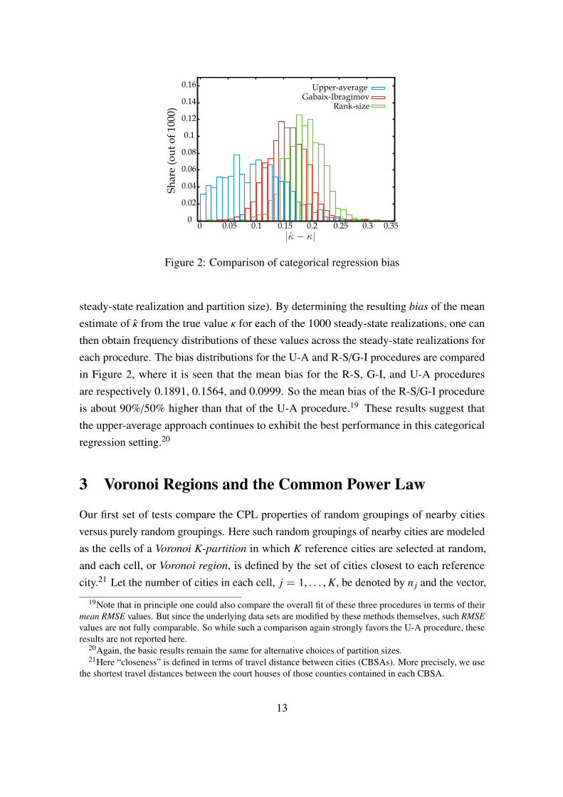
Figure 2: Comparison of categorical regression bias

steady-state realization and partition size). By determining the resulting bias of the meanestimate of from the true value for each of the 1000 steady-state realizations, one canthen obtain frequency distributions of these values across the steady-state realizations foreach procedure. The bias distributions for the U-A and R-S/G-I procedures are comparedin Figure 2, where it is seen that the mean bias for the R-S, G-I, and U-A proceduresare respectively 0.1891, 0.1564, and 0.0999. So the mean bias of the R-S/G-I procedureis about 90%/50% higher than that of the U-A procedure.19 These results suggest thatthe upper-average approach continues to exhibit the best performance in this categoricalregression setting.20

3 Voronoi Regions and the Common Power Law

Our first set of tests compare the CPL properties of random groupings of nearby citiesversus purely random groupings. Here such random groupings of nearby cities are modeledas the cells of a Voronoi K-partition in which K reference cities are selected at random,and each cell, or Voronoi region, is defined by the set of cities closest to each referencecity.21 Let the number of cities in each cell, j = 1, . . . , K, be denoted by n j and the vector,

19Note that in principle one could also compare the overall fit of these three procedures in terms of theirmean RMSE values. But since the underlying data sets are modified by these methods themselves, such RMSEvalues are not fully comparable. So while such a comparison again strongly favors the U-A procedure, theseresults are not reported here.

20Again, the basic results remain the same for alternative choices of partition sizes.21Here “closeness” is defined in terms of travel distance between cities (CBSAs). More precisely, we use

the shortest travel distances between the court houses of those counties contained in each CBSA.

13

n(K) = (n j : j = 1, . . . , K), be designated as the size of the given partition. Then onlyrandom partitions of the same size will be comparable with this partition. So this sizevector, n(K), defines the key parameters governing the tests to be constructed. As oneillustration of these parameters, Figure 3(a) displays an example of Voronoi K-partitionwith K = 4 and with n(4) = (n1, n2, n3, n4) = (182, 254, 261, 233).

In this context, our basic null hypothesis, H0, is that the level of agreement of Voronoipartitions with the CPL property is statistically indistinguishable from that of similarlysized random partitions. As in Section 2.3, this level of agreement is measured in terms ofRMSE for the corresponding categorical regressions in expression (12) above.

For the Voronoi partition in Figure 3(a), the upper-average plots for these four Voronoiregions are shown in Figure 4(a), where the colors of each plot correspond to the partitioncolors in Figure 3(a).

(a) Voronoi partition (b) Random partition

Figure 3: An example of Voronoi 4-partition

14

0 1 2 3 4 5

Region 1Region 2Region 3Region 4

(a) Voronoi partition (b) Random partition

11

12

13

14

15

16

17

0 1 2 3 4 5

Figure 4: Upper-average distributions in Voronoi and random partitions

So to test the null hypothesis, H0, for a given level of K, we proceed in two stages. Firstwe generate M = 1000 random Voronoi K-partitions, v = 1, . . . , M. Associated witheach partition, v, is a given size vector, nv(K). So to estimate the distribution of RMSEfor random partitions of size nv(K) under H0, we generate 1000 random partitions of sizenv(K) and calculate RMSE for each. For the Voronoi 4-partition shown in Figure 3(a), anexample of random partition of the same size is shown in Figure 3(b), with correspondingupper-average plots shown in Figure 4(b). As can be seen from this figure, the upper-averageplots di↵er from the Voronoi partition case mainly in the extreme upper tail, correspondingto the largest cities. In particular, the four largest cities (New York, Los Angeles, Chicagoand Dallas) are contained in separate cells in the Voronoi partition shown in Figure 3(a),while for the random partition shown in Figure 3(b), all the four cities are contained ina single cell (the red region in the figure). As we shall see below, the locations of theselargest cities within a given partition play a crucial role in determining its agreement withthe CPL property.

If the RMSE level for partition v is denoted by RMSEv, and if the number of RMSEvalues smaller than RMSEv is denoted by Mv, then the p-value for a one-sided nonparametrictest of H0 for partition v is given by22

pv =Mv

N, v = 1, . . . , M. (14)

22To be more precise, pv, estimates the probability of achieving an RMSE level as low as RMSEv if it weretrue that partition v was in fact a typical random partition of size nv(K).

15

For the Voronoi partition, v, with upper-average plots in Figure 4(a), the RMSE valueis RMSEv = 0.072, and for the same sized random partition in Figure 4(b), the value isRMSE = 0.162. So this random partition exhibits less agreement with CPL than doespartition v. In fact, for this particular Voronoi partition, none of the RMSE values for thecorresponding 1000 random partitions fell below 0.072. So pv = 0 for this extreme case.

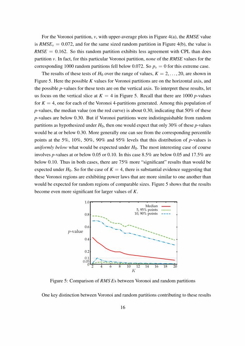
The results of these tests of H0 over the range of values, K = 2, . . . , 20, are shown inFigure 5. Here the possible K values for Voronoi partitions are on the horizontal axis, andthe possible p-values for these tests are on the vertical axis. To interpret these results, letus focus on the vertical slice at K = 4 in Figure 5. Recall that there are 1000 p-valuesfor K = 4, one for each of the Voronoi 4-partitions generated. Among this population ofp-values, the median value (on the red curve) is about 0.30, indicating that 50% of thesep-values are below 0.30. But if Voronoi partitions were indistinguishable from randompartitions as hypothesized under H0, then one would expect that only 30% of these p-valueswould be at or below 0.30. More generally one can see from the corresponding percentilepoints at the 5%, 10%, 50%, 90% and 95% levels that this distribution of p-values isuniformly below what would be expected under H0. The most interesting case of courseinvolves p-values at or below 0.05 or 0.10. In this case 8.5% are below 0.05 and 17.5% arebelow 0.10. Thus in both cases, there are 75% more “significant” results than would beexpected under H0. So for the case of K = 4, there is substantial evidence suggesting thatthese Voronoi regions are exhibiting power laws that are more similar to one another thanwould be expected for random regions of comparable sizes. Figure 5 shows that the resultsbecome even more significant for larger values of K.

10, 90% points

Median 5, 95% points

p-value

2 10 6 8 4 12 16 18 14 20 0

0.2

0.4

0.6

0.8

1.0

0.050.1

Figure 5: Comparison of RMS Es between Voronoi and random partitions

One key distinction between Voronoi and random partitions contributing to these results

16

is that the largest cities tend to be more separated by Voronoi partitions than randompartitions. This separation property will be established more formally in Section 4.1 below.But for the present, the relation between CPL properties and separation of large cities canbe illustrated by focusing on the single significance level, ↵ = 0.05, in Figure 5. If foreach K we denote the set of (simulated) Voronoi K-partitions that are significant at this ↵level by VK

↵ = {v : pv < ↵}, then we can measure the degree of large-city separation inthese partitions as follows. For each partition, v 2 VK

↵ , let NKr (v) denote the number of

cells in partition v containing at least one of the top r cities [so that NK2 (v) is the number

of cells in v containing either New York or Los Angeles]. Finally, if N Kr (↵) denotes the

average of these values over VK↵ [so that 1 N

Kr (↵) r], then the fraction, N

Kr (↵)/r, can

be viewed as measuring the degree of separation of the top r cities in VK↵ . These degrees of

separation are plotted over a range of K values for r = 2, 3, 4 in Figure 6. So at K = 4, forexample, the degree of separation for r = 2 is seen to be 1.0, indicating that every partitionsignificant at the ↵ = 0.05 level (i.e., in V4

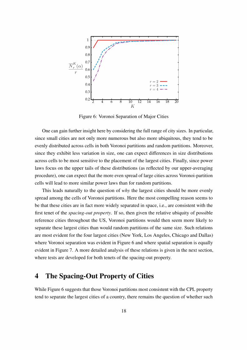
↵) places New York and Los Angeles in di↵erentcells. Similarly, the degree of separation for r = 4, namely 0.78 ⇡ 3/4, indicates that thetop four cities are typically split among three of the four cells in these partitions. Whatis most important for our present purposes is that these degrees of separation for r = 4exhibit a sharp increase from K = 3 to K = 4, and continue to increase for larger K. Thisechoes the decreasing contour for ↵ = 0.05 in Figure 5, and shows that the most significantVoronoi partitions with respect to CPL (at this ↵ level) are indeed those achieving greaterseparation, i.e., with these four cities almost always completely separated.23

23For completeness, it should also be noted that for K = 2, 3 the stronger significance of these partitionsagain depends largely on the patterns of separation between the top four cities. For K = 2, it can be verifiedby closer examination of the partitions in V2

↵ [and can also be seen roughly from Figure 1(a) ] that separationsin which New York is in one cell and (Los Angeles, Chicago, Dallas) are in the other will tend to yield verysimilar upper-average curves for a considerable range of di↵erent Voronoi 2-partitions.

17

2 4 6 8 10 12 14 16 18 20 0.2

0.3

0.4

0.5

0.6

0.7

0.8

0.9

1

Figure 6: Voronoi Separation of Major Cities

One can gain further insight here by considering the full range of city sizes. In particular,since small cities are not only more numerous but also more ubiquitous, they tend to beevenly distributed across cells in both Voronoi partitions and random partitions. Moreover,since they exhibit less variation in size, one can expect di↵erences in size distributionsacross cells to be most sensitive to the placement of the largest cities. Finally, since powerlaws focus on the upper tails of these distributions (as reflected by our upper-averagingprocedure), one can expect that the more even spread of large cities across Voronoi-partitioncells will lead to more similar power laws than for random partitions.

This leads naturally to the question of why the largest cities should be more evenlyspread among the cells of Voronoi partitions. Here the most compelling reason seems tobe that these cities are in fact more widely separated in space, i.e., are consistent with thefirst tenet of the spacing-out property. If so, then given the relative ubiquity of possiblereference cities throughout the US, Voronoi partitions would then seem more likely toseparate these largest cities than would random partitions of the same size. Such relationsare most evident for the four largest cities (New York, Los Angeles, Chicago and Dallas)where Voronoi separation was evident in Figure 6 and where spatial separation is equallyevident in Figure 7. A more detailed analysis of these relations is given in the next section,where tests are developed for both tenets of the spacing-out property.

4 The Spacing-Out Property of Cities

While Figure 6 suggests that those Voronoi partitions most consistent with the CPL propertytend to separate the largest cities of a country, there remains the question of whether such

18

separation is exhibited by all Voronoi partitions. If so, then as suggested above, this wouldprovide strong evidence for the first tenet of the spacing-out property. In Section 4.1below we develop a testing procedure that confirms the presence of such separation quiteindependently from any considerations of the CPL property.

In addition, we show the spacing-out property also asserts that smaller cities tend to beclustered around these larger centers. In Section 4.2 below we show that Voronoi partitionsgenerated by the largest cities do indeed exhibit significantly stronger accessibility to thesmaller cities in their cells than do Voronoi partitions generated by random cities. Theseresults thus provide further support for the spacing-out property itself.

4.1 Spatial Separation of the Largest Cities

Let U denote the relevant set of cities for a given country (so that |U | = 930 for the caseof US). For any given number, r, of the largest cities in U, and for any partition, v, ofU, let Nr(v) denote the number of partition cells of v containing at least one of these rcities. If there is indeed substantial spacing between the largest cities in U, then we wouldexpect Nr(v) to be larger for Voronoi partitions than for random partitions of the same size.For given values of r and K, we start by simulating M (= 1000) Voronoi K-partitions,v = 1, . . . , M, as in Section 3, and summarize the above counts, Nr(v) , by the Voronoicount vector,

Nr = [Nr(v) : v = 1, . . . , M] . (15)

For each of these Voronoi K-partitions, v, we again simulate M (= 1000) random K-partitions, ! = 1, . . . , M, of the same size, nv(K). But rather than conducting separatetests for each Voronoi partition, v, as in Section 3, we now construct a summary test usingappropriate mean values as follows.

First we write the random partitions for v as ordered pairs (v,!), ! = 1, . . . , M, toindicate their size-dependency on v. In a manner paralleling Nr(v), we then let Nr(v,!)denote the number of cells in random partition (v,!) that contain at least one of the rlargest cities in U. In these terms the count vectors,

Nr(!) = [Nr(v,!) : v = 1, . . . , M] , ! = 1, . . . , M (16)

can each be regarded as random-partition versions of the Voronoi count vector in (15),where each component, Nr(v,!) , of Nr(!) is based on a random partition of the samesize as Voronoi partition, v. In this setting, our basic null hypothesis is essentially that theVoronoi count vector, Nr is drawn from the same population as its random-partition versions

19

in (16). But for operational simplicity, we focus only on the associated mean-counts, definedfor (15) and (16), respectively, by

Nr =1M

MX

v=1Nr(v) (17)

and

Nr(!) =1M

MX

v=1Nr(v,!) , ! = 1, . . . , M . (18)

In these terms, our explicit null hypothesis, H0, is that the Voronoi mean-count, Nr, is drawnfrom the same population as its associated random mean-counts, Nr(!), ! = 1, . . . , M.24

If for the given set of simulated random partitions above, we now let M0 denote the numberof random mean-counts, Nr(!), larger than Nr, then the p-value, p0, for a one-sided test ofH0 is given [in a manner similar to (14)] by

p0 =M0

M. (19)

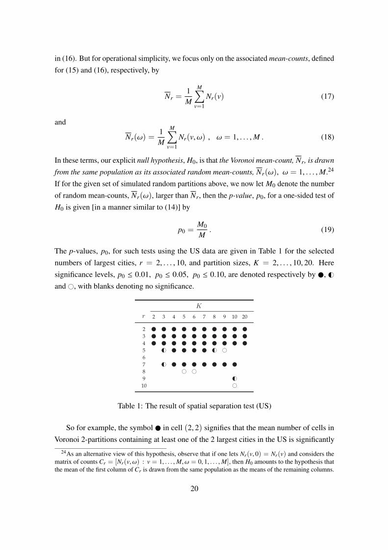
The p-values, p0, for such tests using the US data are given in Table 1 for the selectednumbers of largest cities, r = 2, . . . , 10, and partition sizes, K = 2, . . . , 10, 20. Heresignificance levels, p0 0.01, p0 0.05, p0 0.10, are denoted respectively by , G#and #, with blanks denoting no significance.

5 103 204 62 7 8 9

2

5

10

34

6789

Table 1: The result of spatial separation test (US)

So for example, the symbol in cell (2, 2) signifies that the mean number of cells inVoronoi 2-partitions containing at least one of the 2 largest cities in the US is significantly

24As an alternative view of this hypothesis, observe that if one lets Nr(v, 0) = Nr(v) and considers thematrix of counts Cr = [Nr(v,!) : v = 1, . . . , M,! = 0, 1, . . . , M], then H0 amounts to the hypothesis thatthe mean of the first column of Cr is drawn from the same population as the means of the remaining columns.

20

greater (at the 0.01 level) than would be expected if this were a random 2-partition. More-over, since for r = 2, this significance level persists for all partition sizes up to K = 20, itis evident that for Voronoi 2-partitions these two largest cities (New York and Los Angeles)are almost never in the same cell of any such partition. This is hardly surprising, sinceNew York and Los Angeles are on opposite coasts. So the key point here is that randompartitions are not sensitive to “opposite coasts”, while Voronoi partitions most certainly are.More generally this same degree of maximal significance is seen to persist up to the firstfour largest cities (New York, Los Angeles, Chicago, and Dallas), which we have alreadyseen are spaced widely apart within the US. But when the fifth largest city (Philadelphia)is included, its close proximity to New York makes such separation less likely. Moreover,since the sixth largest city (Houston) is also close to Dallas, the significance of Voronoiseparation now disappears altogether. What is more interesting is the apparent resurgenceof significance when the seventh largest city (Miami) is included. Here again it is evidentfrom the map in Figure 7 that Miami is about as far away from the six largest cities as isphysically possible within continental US.

Boston (10)New York (1)Philadelphia (5)

Washington, DC (8)

Miami (7)Houston (6)Dallas (4)

Los Angeles (2)

Chicago (3)

Atlanta (9)

Figure 7: Locations of Cities

So again, this separation e↵ect is strongly captured by our testing procedure. Insummary, these results do indeed support the spacing-out property of largest cities withinthe US, and in particular, they echo the strong separation of the four largest cities seen inthe tests of Section 3 above. Notice also that the spacing between these largest four cities issomewhat more uniform than the spacing between smaller cities. This is in part explainedby the the tendency of smaller cities to cluster around larger cities, as we examine furtherin the next section.

21

4.2 Concentration of Smaller Cities Around the Largest Cities

We now focus on the spatial distribution of smaller cities associated with that of the largestcities studied in the previous section. For this purpose, we designate the (unique) VoronoiK-partition generated by the K largest cites as the largest-city Voronoi K-partition. Ourobjective is then to test whether these K largest cities are significantly more accessible toall other cities in their cells than are the corresponding reference cities in random VoronoiK-partitions (as in Section 3 above).

To formalize these concepts, we first identify the sets of cities in each partition cell. Forany Voronoi K-partition, let the set of all cities in each cell, i = 1, . . . , K, be denoted byUi (⇢ U), and let ui 2 Ui denote the reference city in this cell. If the distance from ui toany city u 2 Ui is denoted by d(ui, u),25 then the total distance of all cities in U to theirreference cities in a given Voronoi K-partition is then given by

DK ⌘KX

i=1

X

u2Ui

d(ui, u) . (20)

With these definitions, if the largest K cities do indeed serve as cluster centers for thosesmaller cities around them, then one should expect to observe values of DK for largest-cityVoronoi K-partitions that are smaller than the corresponding values, say eDK , for similarlysized random Voronoi K-partitions. To test this assertion for a given value of K = 2, 3, . . ., the appropriate null hypothesis, H0, is simply that DK and eDK come from the samestatistical population. By using the 1000 samples of random Voronoi K-partitions as in theprevious section, we can then compute the appropriate p-value for a one-sided the test ofH0 for this value of K.

Alternatively, it may be more appropriate to use accessibilities to city populations byweighting each distance, d(ui, u), in eq. (20) by the population size, su, of city u 2 Ui .Note however that since d(ui, ui) = 0 for each reference city, ui, the populations of the Klargest cities will automatically be excluded from the largest-city Voronoi K-partition. Butfor random K-partitions, where these largest cities are generally not the reference cities,these largest populations will often be included in total population-weighted distances.Thus in order to focus on comparisons of accessibility to populations in smaller cities, it isappropriate to exclude the K largest city populations from all such comparisons.26 To do

25Recall that our measure of distance, d(u, u0), between cities u and u0 was defined in footnote 21 above.Note in particular that this (set) distance implies that the distance from any city to itself is zero, i.e., thatd(u, u) = 0.

26As will become clear below, this convention has the additional advantage of yielding a conservative testof clustering around the largest cities. In particular, the inclusion of largest-city populations must necessarily

22

so, if we now denote the set of K largest cities in U by UK , then for any given largest-cityVoronoi K-partition, the appropriate modification of DK above is now taken to be the totalpopulation-weighted distance as defined by,

D⇤K ⌘KX

i=1

X

u2Ui�UK

sud(ui, u) . (21)

If the total population-weighted distance for a random K-partition is similarly denoted byeD⇤K , then the appropriate null hypothesis, H⇤0, for this alternative test is now that D⇤K andeD⇤K come from the same statistical population.

Since the largest-city Voronoi K-partition is unique for each K, the hypotheses, H0 andH⇤0, are tested by simulating 1000 random Voronoi K-partitions and calculating appropriatep-values (for one-sided tests) as the share of associated total distance values, eDK < DK ,under H0, and the share of total population-weighted distance values, eD⇤K < D⇤K , under H⇤0,respectively. The results of these tests are plotted in Figure 8 for K = 1, . . . , 20. Turningfirst to H0 (plotted in red), the significance results for K = 3 and 4 reflect the strongtendency in Voronoi separation for r = 3 and 4 in Table 1. Note that high p-value at K = 2is expected. For since the largest two cities (New York and Los Angeles) are located onopposite coasts, random pairs of reference cities will almost always have better overallaccess to cities than these two. The subsequent rise in p-values at K = 5 and 6 echoesthe spatial separation results for r = 5 and 6 in Table 1. In particular, given the respectivecloseness of Philadelphia to New York and Houston to Dallas, the addition of each of thesereference cities yields only a small increase in overall accessibility relative to randomlychosen reference cities. Similarly, the improvement in accessibility when Miami is added(K = 7), and deterioration when Washington, D.C. is added (K = 8) also reflect the casesof r = 7 and 8 in Table 1. But overall, there is a discernible tendency of cities to exhibitmore clustering around the largest cities than around randomly selected reference cities.

This tendency is much more dramatic when population accessibilities are compared.As shown by the blue curve in Figure 8, these results are uniformly more significant thanfor the case of simple inter-city distances. Indeed, except for the “bi-coastal” case (K = 2)and the “Houston next to Dallas” case (K = 6), these results are all strongly significant(p ⌧ .05). Thus, the single most important conclusion here is that relative to randomlyselected reference cities, the largest cities in the US tend to exhibit significantly betteraccess to their surrounding city populations.

In relation to the results in Section 3 above, the spatial relations between smaller and

increase the total population-weighted distances for almost all random K-partitions.

23

larger cities studied here show that the city subsets around the three or four largest cities areroughly comparable to one another, each consisting of similarly sized cities. This in partsuggests why Voronoi partitions tend to exhibit higher consistency with the CPL propertythan their random counterparts. In particular, those Voronoi cells containing the largestcities tend also to contain substantial portions of their corresponding city clusters.

0.8

1.0

0.6

0.4

0.2

00.050.10

p-va

lue

2 10 6 8 4 12 16 18 14 20

Geographical accessibilityPopulation accessibility

Figure 8: Result of total-accessibility test

5 Economic Regions and the Common Power Law

Our final objective is to determine whether the CPL property is stronger when comparingmore economically meaningful regions. As mentioned in the Introduction, we here replacesimple distance proximities by commodity flow dependencies. Such dependencies arebased on the Commodity Flow Survey (CFS) for 2007. This data identifies total shipmentsbetween 111 regions in the continental US, as defined by the CFS. In particular, 64 of theseregions are CFS-defined metropolitan areas, and the remaining 47 regions are either statesthat do not overlap these metropolitan areas or “remainder of the state” regions includingthose part of states outside the metro areas.27 Each CFS metropolitan area is either anindividual CBSA, or a Combined Statistical Area (CSA) consisting of multiple CBSAs.28

27The 47 regions correspond to the continental states excluding Rhode Island as it is completely containedin a CFS-defined metro area, Boston-Worcester-Manchester.

28However, there is one case in which a single CBSA (Washington-Arlington-Alexandria) has been di-vided into two CFS metropolitan areas [designated, respectively, as the Washington-Arlington-AlexandriaCBSA and the Washington-Baltimore-Northern Virginia CSA (Virginia part)]. In order to recon-cile this CFS data with the set of CBSAs defining “cities” in the present paper, we have thus ag-gregated these two CFS areas into a single Washington-Arlington-Alexandria metropolitan area (con-sisting of three CBSAs, Washington-Arlington-Alexandria, Winchester and Culpeper). For the com-

24

We start in Section 5.1 below by constructing an operational definition of economicregions in terms of these commodity flow dependencies. In Section 5.2, we then test thesignificance of the CPL property for these economic regions against comparable sets ofrandom partitions. In Section 5.3 these CPL test results are shown to be even strongerthan comparable results for the Voronoi partitions in Section 3. Finally in Section 5.4, wedevelop an alternative method for comparing di↵erences in upper-average distributionsbetween economic regions and between their corresponding random partitions. In particular,we construct a new measure of similarity of between upper-average distributions in termsof the order-consistency properties of their ULS i levels across ranks, i. Here it is shownthat this measure can in many cases provide even sharper comparisons between power lawsacross regions.

5.1 Economic Regions

If R denotes the set of all CFS regions, i = 1, . . . , 111, we first identify each region, i 2 R,with its associated set of cities as follows. Let the set of all cities, U, be partitioned intocells, {Ui : i 2 R}, so that u 2 Ui if and only if region i accounts for the largest populationshare of city u. In the analysis to follow we refer to Ui as the set of cities for region i. Forconvenience we then order regions in terms of their largest cities, so that by again lettingsu denote the size of city u it follows that regions, i, j 2 R, will satisfy i < j if and only ifmaxu2Ui su > maxu2U j su. Thus the first K regions will generally be associated with the Klargest cities in U.29 For each K (= 1, 2, . . .), the desired sets of K economic regions thencorrespond essentially to the largest-city regions together with their associated economichinterlands.

These ideas can be made more precise terms of commodity-flow dependencies asfollows. If for any regions, i, j 2 R, we let fi j denote the commodity flow (in dollar value)from region i to region j, then the (commodity) flow dependency, �i j 2 [0, 1), of region j onregion i is taken to be the fraction of the total commodity-inflow to j that comes from i, i.e.,

�i j ⌘fi j

P

k2R fk j, (22)

plete list of the CFS metropolitan areas, refer to the website of the US Department of Transportation:http://www.rita.dot.gov/bts/sites/rita.dot.gov.bts/files/publications/commodity flow survey/2007/ metropoli-tan areas/index.html.

29In particular, the largest cities in the first K = 20 regions (used in the analysis below) match the largest 20cities in U, with the two exceptions of Los Angeles-Long Beach-Santa Ana (second largest) and Riverside-SanBernardino-Ontario (14th largest) that belong to the same CFS region.

25

where in particular, � j j is designated as the self-flow dependency of region j. For anygiven set of K “central” regions, one can then generate appropriate economic hinterlandsby simply assigning every other region in R to its largest supplier among these K regions.But the definition of “central” regions themselves is more subtle. Here it might seemnatural to simply choose the first K regions, i.e., with the largest cities. But this ignores therelative flow dependencies among these regions. For example, while Philadelphia is thefifth largest city, it exhibits a strong flow dependency on New York (�1,5 = 0.119). Thissuggests that in central-region systems with K � 5, it might be more appropriate to treatPhiladelphia as part of the New York hinterland. More generally, the notion of “centrality”itself appears to involve a tradeo↵ between flow dependencies and largest-city sizes. Tomake this tradeo↵ explicit, we now parameterize possible collections of K central regionsin terms of the maximum allowable flow dependency between any pair of central regions,designated as their threshold-dependency level, � 2 (0, 1). For any given values of � andK, we then define the appropriate set of central regions, R�,K , to be the first K regions,j 2 R, with no flow dependencies on larger regions that are higher than either � or theirown self-flow dependency, � j j.30,31 To be more precise, if we now let R⇤j = {i 2 R : i < j}denote the set of regions with larger maximum city size than region, j, then membership inR�,K ⌘ { jm : m = 1, . . . , K} ⇢ R is defined by j1 = 1 and for all m = 2, . . . , K by

jm = arg min

8

>

>

<

>

>

:

j > jm�1 : maxi2R⇤j�i j min{�, � j j}

9

>

>

=

>

>

;

. (23)

In essense, central regions, R�,K , constitute the set of K largest regions exhibiting nomutual flow dependencies stronger than �. Note however that parameters, K and �, areby no means independent. In particular, for su�ciently small values of �, only K = 1is possible, i.e., the entire country is in the economic hinterland of New York. However,

30Note that one could in principle require the first condition to hold for all other regions rather thansimply larger regions. However, there are exceptions where smaller regions are the largest suppliers oflarger regions, especially when the smaller region is a major transshipment point (such as a port) or a borderregion. The most important instance for our purposes is Houston ( j = 6), which is a major supplier ofDallas ( j = 4). For example at the � = 0.05 level, it can be seen from Table 3 in the Appendix that�4,6 = 0.036 < � < 0.055 = �6,4, which would exclude Dallas as a central region for this level of �. So toavoid such exceptional cases, we apply this condition only to larger regions. But it should also be noted herethat such di�culties are in part due to the fact that CFS data does not distinguish transshipment points fromorigin and destination points, thus tending to overestimate outflows originating at transshipment points.

31Note also that while the second condition is reasonable, it is actually only binding for one CFS region. Inparticular, San Diego-Carlsbad-San Marcos imports 36.4% from Los Angeles-Long Beach-Riverside, whileits domestic supply (self-flow dependency) accounts for only 29.9%. But since San Diego-Carlsbad-SanMarcos hardly constitutes an economic center comparable to Los Angeles-Long Beach-Riverside, this createsno problem for the present analysis.

26

for first 20 regions in R considered in the present analysis, all relevant numbers of centralregions, 2 K 20, are possible for threshold-dependency levels, � � 0.05. Finally,it should be clear that even in this most relevant range, the set of central regions, R�,K ,can be quite di↵erent from the first K regions in R. These di↵erences are of course mostdramatic for small �. In the case of � = 0.05, for example, four of the ten largest regions(Philadelphia, Miami, Washington DC, and Boston) are all excluded by their strong flowdependencies on New York. Additional details and examples can be found in the Appendix,where all flow dependencies among the first 20 regions in R are depicted in Table 3.

Given this definition of central regions, R�,K , we can now define the associated system ofeconomic regions, E�,K , as follows. For each central region, j 2 R�,K , let the correspondingeconomic region, E j, consist of all regions in R for which region j is the largest supplier,i.e.,

E j ⌘(

i 2 R : j = arg maxr2R�,K

�ri

)

. (24)

This automatically generates a K-partition of U under threshold-dependency level, �,

E�,K ⌘n

E j : j 2 R�,Ko

, (25)

which we now designate as the economic-region K-partition for �.

27

Miami

Philadelphia

New York regionLos Angeles region

Chicago regionDallas region

Philadelphia regionHouston region

Atlanta region

Atlanta

Houston

Chicago

New York

Los AngelesDallas

St. Louis

Figure 9: Economic regions for selected values of � and K

These economic-region partitions are illustrated by the examples in Figure 9 for selectedcombinations of � and K. Here each colored cell represents the geographical coverage ofa single city in U. Those cities of the same color all belong to a single economic region.In particular, panel (a) shows the economic-region 4-partition, E0.1,4, that happens to bethe same for all � 2 [0.037, 1.0]. Here the corresponding central regions, R�,4, consist ofthe four largest cities (New York, Los Angeles, Chicago and Dallas). Notice the strongresemblance between these four economic regions and Voronoi 4-partition in Figure 3(a).

5.2 Test of the CPL Property

To test the significance of the CPL property for the economic regions, we constructedeconomic-region partitions, E�,K , for selected values of (�, K), and (as in Section 3)generated 1000 random partitions of similar sizes for each case.32 The relevant range ofsignificant results are shown in Table 2, where each cell contains the p-value (p0) for a

32The values of � used were (i) 0.05 to 0.15 in increments of 0.01, and (ii) 0.20 to 1.00 in increments of0.10. The values of K used were K = 2, . . . , 20. Note also that while it is possible to consider values � < 0.05in some cases, these flow dependency thresholds are so low that the resulting economic regions tend exhibitlittle spatial cohesion whatsoever.

28

one-sided test of H0 given that particular (�, K) pair.33 As in Table 1, significance levels,p0 0.01, p0 0.05, p0 0.10, are denoted respectively by , G# and #, with blanksdenoting no significance. To interpret these results, we first note that since the four largestcities are highly independent of one another in terms of commodity flows (as shown in Table3 of the Appendix), the economic-region partitions, E�,K , are the same for all � � 0.05when K 4.34 Thus the test results shown in the first three columns continue to hold forall � � 0.12, as indicated in the table. In particular, the economic-region partitions forboth K = 3 and 4 are significantly more consistent with the CPL property than randompartitions regardless of mutual flow-dependency considerations.35 (The insignificance ofCPL for the K = 2 case will be discussed in Section 5.3 below.)

To examine these results in more detail, it is instructive to compare the upper-averagedistributions of economic-region partitions with representative random partitions of thesame size. The upper-average distributions of E�,K for K = 4 (and all � � 0.05) areshown in panel (a) of Figure 10. To represent random partitions of the same size, we usethe random partition with median RMSE value, as shown in panel (b). As in the Voronoi4-partition example of Figure 4 in Section 3, the distinction between observed and randompartitions is again seen to be most pronounced in the upper tails of the distributions. Notein particular that for the largest 100 cities (i.e., up to ULRi = 3.64), the upper-averagedistributions for these four economic regions do not cross one another, while many suchcrossings occur in the corresponding random partition.36

33The only significant cases not shown (namely with � = 0.06, 0.07 and K � 18 ), all include single-cityregions for which power laws are not meaningful.

34To be more precise, R�,4 consists of the largest four cities for all � > 0.037, while Dallas will be containedin Los Angeles region for � 0.037. Similarly, R�,3 consists of the largest three cities for all � > 0.029, whileChicago will be contained in New York region for � 0.029. Refer to Table 3 in the Appendix for thesethreshold levels of �.

35Notice that even under di↵erent values of threshold-dependency levels, say, � and �0, the economic-regionpartitions are identical, i.e., E�,K = E�0,K , if the set of central regions are identical, i.e., R�,K = R�0,K .

36Such comparisons will be made more explicit in Section 5.4 below.

29

53 4 62 7

0.050.060.070.080.090.100.11

Table 2: Result of CPL test for economic regions

11

12

13

14

15

16

17

18

0 1 2 3 4 5 0 1 2 3 4 5

(a) Actual (b) Random median

New YorkLos Angeles

ChicagoDallas

Figure 10: Upper-average distributions under (�, K) = (0.1, 4)

For K � 5, the CPL property continues to be significant until either Philadelphia(the 5th largest) or Atlanta (the 9th largest) is added as a central region. As mentionedabove, Philadelphia belongs to the hinterland of New York when � 0.119, but forms itsown economic region at all higher values of �. Similarly, Atlanta belongs to the Chicagohinterland for � 0.032 , but forms its own economic region at all higher levels. Thepresence or absence of these two cities appear to be the major factors governing the patternof significance levels for K � 5 in Table 2.

The “Atlanta e↵ect” can be illustrated by the case, (�, K) = (0.05, 6), shown in Figure9(b), which is relatively close to the K = 4 case but no longer exhibits any significant

30

consistency with the CPL property. To understand this dramatic di↵erence, note first that thesix central cities include the four largest cities together with Houston and Atlanta.37 Hereboth Philadelphia and Miami now belong to the New York region, even though Philadelphiais larger than Houston, and Miami is larger than Atlanta. Notice also that the New Yorkregion for this case is about a half its size under K = 4 in Figure 9(a), where the southernhalf is now taken by Atlanta except for the isolated city of Miami. As a consequence, thereare too few small cities in the economic region of New York to sustain the CPL propertywith other economic regions. As seen in Figure 11, this is reflected in the upper-averagedistribution of the New York region, which now exhibits strong concavity in the lower tailcompared to that shown in Figure 10(a) for (�, K) = (0.1, 4).

11

12

13

14

15

16

17

18

0 1 2 3 4 5

New YorkLos Angeles

ChicagoDallas

HoustonAtlanta

Figure 11: Upper-average distributions under (�, K) = (0.05, 6)

Next, the “Philadelphia e↵ect” is well illustrated by the case, (�, K) = (0.12, 5), inFigure 9(c). Notice that the coverage of the Philadelphia region is very limited.38 As aconsequence, the upper-average distribution of this region di↵ers markedly from thoseof other regions, as seen in Figure 12. This in turn deteriorates the strength of the CPLproperty seen at lower levels of �.

37To be more precise, the same 6-partition as depicted in Figure 9(b) is obtained for all � 2 (0.037, 0.052].In particular, among the central cities in R0.05,6, Dallas would belong to the hinterland of Los Angeles for

� 0.037, while Miami (which is larger population size than Atlanta) belongs to the hinterland of New Yorkfor � 0.052, but would join R�,6 for � > 0.052 in place of Atlanta.

38Notice also that the set of five central cities is identical for all � � 0.12, since the threshold-dependency,�, is relevant only for the selection of the central cities.

31

11

12

13

14

15

16

17

18

0 1 2 3 4 5

New YorkLos Angeles

ChicagoDallas

Philadelphia

Figure 12: Upper-average distributions under (�, K) = (0.12, 5)

Thus, while the case of K = 4 yields strong consistency with the CPL property acrossall values of � , the above examples show that for larger values of K, the addition ofeconomic regions with smaller central cities tends to increase the variation among upper-average distributions, leading to a deterioration of the CPL property. However, it shouldalso be noted that this deterioration may in part be due to our partition-based definition ofeconomic regions. In reality such regions tend to overlap, and may even form hierarchicalrelations. For example, rather than requiring Philadelphia to form a separate region at higherlevels of commodity-flow dependency, it may be more appropriate to treat Philadelphia as asubcenter within the New York region. Along these lines, it has been shown by Akamatsuet al. [3] (using the same data as ours) that such hierarchical economic regions yield evenstronger support for the CPL property (as discussed further in the Conclusions).

5.3 Comparison with Voronoi Partitions

It is also of interest to compare these CPL results with those obtained in Section 3 forthe simpler case of Voronoi partitions. This comparison is shown in Figure 13, where the5% and 10% bands for Voronoi partitions in Figure 5 are here reproduced (in green andblue, respectively). The significance levels (p-values) for economic-region partitions with� = 0.1 and K = 2, . . . , 20 are then superimposed (in red) on these bands (where the grayband can be ignored for the moment). Before comparing the more significant results, webegin by noting the conspicuous lack of significance for economic regions at the K = 2level, in contrast to the Voronoi results. Closer examination of this case shows that while

32

0

0.1

0.2

0.3

0.4

0.5

2 4 6 8 10 12 14 16 18 20

Random Voronoi (5% point)Random Voronoi (10% point)

Economic regions (λ = 0.1)Largest-city Voronoi

p-value

K

Figure 13: CPL Comparisons of Economic-Region and Voronoi Partitions

many Voronoi 2-partitions tend to split the country evenly between New York and LosAngeles (given the higher density of possible reference-city pairs on the two coasts), theeconomic-region 2-partition case is actually somewhat more random. In particular, thosecities in the third major economic region, Chicago, are split quite randomly according towhich flow dependency on New York or Los Angeles is the larger one, leading to lessspatial coherence of these two regions. In contrast, the similarities between these threemajor regions are fully reflected at the K = 3 level, leading to results comparable tothe top 5% of Voronoi cases. Moreover, for the most important cases of K = 4 through6 (as discussed above) there is far stronger consistency with the CPL property than forcomparable Voronoi cases. In particular, the p-values here are actually below the 1% band(not shown), indicating that the CPL property is more significant for these economic-regionpartitions than for 99% of the 1000 randomly generated Voronoi partitions.

However, one may ask whether these results might not be improved by using largest-cityVoronoi partitions rather than random choices. So as one final comparison, the p-valuesfor the K largest-city Voronoi partitions, K = 2, . . . , 20, are shown by the gray bandin Figure 13. Surprisingly these results are never more than weakly significant, and inaddition, are nowhere close to the top 10% of the randomly generated Voronoi partitions.Recall from Figure 8 however that in terms of the spacing-out property, these largest-city Voronoi partitions exhibit significantly higher population accessibility (lower totalpopulation-weighted distances) than do random Voronoi partitions. Moreover, they alsotend to exhibit higher population accessibility than economic-region partitions for any givenK. In particular, when largest-city Voronoi partitions share the same reference cities as

33

New York

Chicago

St. Louis

Miami

Dallas

New York regionLos Angeles region

Chicago regionDallas region

Figure 14: The largest-city Voronoi 4-partition

economic-region partitions (as for example when � = 0.1 and K 4) then by constructionthey must exhibit higher population accessibility.39

But given the stronger CPL properties of economic-region partitions, it is of interest toask how these two types of partitions di↵er when their reference cities consist of the samelargest cities. In general terms, since the cells of both partitions tend to include those citiesclosest to each largest city, the major di↵erences are near the boundaries of each cell. Acloser look at the data indicates that for those major cities relatively far from any of the Klargest cities (i.e., those near the regional boundaries), their largest trade partners are oftennot the closest of the K largest cities. This can be illustrated for K = 4 by a comparisonof the economic-region partition (for � = 0.1) in Figure 9(a) with the largest-city Voronoipartition shown in Figure 14. For example, while Miami is closest to Dallas [i.e., is in thegreen region of Figure 14], its largest flow dependency is on New York [i.e., is in the redregion of Figure 9(a)]. Similarly, St. Louis is closest to Chicago [i.e., is in the magentaregion of Figure 14], but again with largest flow dependency on New York [i.e., is also inthe red region of Figure 9(a)]. These observations suggest that in terms of the CPL propertyitself, perhaps a trade-linkage interpretation of the spacing-out property would be moreappropriate than our present geographical version.

5.4 Order-Consistency of Upper-Average Distributions

Recall from the example in Figure 10 that a distinguishing feature of economic-regionpartitions exhibiting significant CPL properties is that their upper-average distributionsappear to be more “parallel” than those of comparable random partitions. This e↵ect can

39Since each non-reference city in a Voronoi partition must always be assigned to its closest reference city,it follows by definition that both distance sums in (20) and population-weighted distance sums in (21) arenecessarily minimal with respect to the given set of reference cities.

34

1 2 3 41 0 01

12

Figure 15: Categorical Regression Example

be described more formally in terms of the order consistency among these upper-averagedistributions, i.e., the order consistency among the ULS i values at each rank value i. As wenow show, this type of consistency is far more stable for economic-region partitions thanfor random partitions as shown below.

To do so, we begin by observing that if all upper-average curves for a given regionalpartition were perfectly parallel (and thus were exactly consistent with the CPL property)then the vertical ordering of ULS values at each rank value would necessarily agreewith their common ordering predicted by the categorical regression used to test this CPLproperty. So the simplest way to measure overall order consistency is to compare theseorderings at each rank value with the common predicted ordering. A stylized version ofsuch comparisons is shown in Figure 15, where only two sets of “red” and “blue” citiesare shown, each consisting of four cities (so that comparisons can be made at all four rankvalues, i = 1, 2, 3, 4). Here the red and blue lines correspond to the results of the categoricalregression (which by construction yields that pair of parallel lines minimizing the overallsum of squared errors for both sets of cities). So the ULS values for blue cities are herepredicted to be above those for red cities at every rank. This is seen to be true at ranksi = 3, 4, but not true at ranks i = 1, 2. So of the possible comparisons that can be madein this case, one can say that the degree of order consistency is 50%. However, for muchlarger examples, it is more convenient to focus on inconsistencies, which tend to be fewerin number and to exhibit wider relative variations. Thus in the present example, the degreeof order inconsistency is also 50%. This is essentially the test statistic we seek to construct.

35

To formalize these ideas for a given number of partition cells, K, let the set of citiesin each partition cell, k = 1, . . . , K, be designated as the kth city set, Uk, of size |Uk|(in a manner paralleling Section 5.1 above). Thus in the example of Figure 15 there aretwo city sets of equal size, |U1| = 4 = |U2|. But more generally, these sets will be ofdi↵erent sizes. So for each city rank, i, the only city sets, Uk, for which this rank ismeaningful are those for which |Uk| � i. If this collection of city sets is now denoted byUK(i) = {k 2 {1, . . . , K} : |Uk| � i}, then the relevant ordering of ULS i values involvesonly those city sets in UK(i). With this in mind, recall next from Section 2.3 that city sets,k, now constitute the appropriate “regions”, j, in expression (12), so that ULS ik denotes therelevant ULS i value for each city set, k 2 UK(i). In these terms the i-rank, ri(k), of cityset, k 2 UK(i), is given by the number of such city sets with ULS i values no larger thanthat of k, i.e., by

ri(k) =�

�

�{` 2 UK(i) : ULS ik ULS i`}�

�

� (26)

so that the city set with highest ULS i value has rank one (assuming no ties). This in turnyields the desired i-rank ordering,

ri(k) ri(`) , ULS ik � ULS i` (27)

for all k, ` 2 UK(i) and i = 1, . . . , n (= |U | ).Given these definitions, our main objective is to compare each ordering in (27) with the

common ordering generated by the categorical regression for partition, K. To do so, recallfrom expression (12) that if (for convenience) we now set �1 = �1 = 0 for the referenceregion, k = 1, then the predicted values, [ULS ik, in this regression are given by

[ULS ik = ↵+ ✓ULRi +mX

h=1�hD j(h) = (↵+ ✓ULRi ) + �k . (28)

Thus the ordering of these predicted values reduces to the identity,

[ULS ik �[ULS i` , �k � �` (29)

which is seen to be independent of i. This in turn yields regression ranks,

r(k) = |{` = 1, . . . , K : �k �`}| (30)

36

which generate the desired regression-rank ordering,

r(k) r(`) ,[ULS ik �[ULS i`, (31)

for all k, ` 2 UK(i) and i = 1, . . . , n.Finally, to determine the degree of inconsistency between this regression-rank ordering

and each i-rank ordering in (27), note first that since we are primarily interested in com-parisons of these orderings in the upper-tail (where CPL properties are most critical), it isnot essential to consider all possible i-rank orderings. In particular, for any given cut-o↵level, I n, one may choose to consider only the I top ranked cities, i = 1, . . . , I. (In theanalysis to follow, we set I = 100.) Next observe that if for each i I and k 2 UK(i) welet Ri(k) = {` 2 UK(i) : ` > k}, then the total number of distinct comparisons to be madeis given by NK(I) =

PIi=1P

k2UK(i) |Ri(k)|. Moreover, observe that for any ` 2 Ri(k), adisagreement occurs between the orderings of ri and r if and only if the signed di↵erences,sgn[ri(k) � ri(`)] and sgn[r(k) � r(`)], are not equal (including possible zeros).40 So if welet �(x, y) = 1, sgn(x) , sgn(y) , and �(x, y) = 0 otherwise, then the desired degree oforder inconsistency is given by the following fraction of disagreements,

�K(I) ⌘1

NK(I)

IX

i=1

X

k2UK(i)

X

`2Ri(k)

�(ri(k) � ri(`), r(k) � r(`)) . (32)

Note in particular that � = 0 if the upper-average distributions of partition cells never crossone another.

To employ �K(I) as a test statistic for a given K-partition, here we consider only the top100 cities (I = 100) and compute �K(100) for this partition.41 Our null hypothesis, H0, isagain that this value is not statistically distinguishable from those values, e�K(100), derivedfrom random K-partitions of the same size (as in Section 5.2 above). To construct a one-sided test of H0, we again sample 1000 random K-partitions of the same size, and estimatethe p-value for this test by the fraction ofe�K(100) values smaller than �K(100). The resultsof these tests for the relevant range of partition sizes, K = 2, . . . , 7, and commodity-flowthresholds, � 2 [0.05, 0.13], are shown in the left panel of Figure 16.42 For purposes ofcomparison, the ratios of the actual �K(100) values to the medians, �K(100), of theircorresponding random �-values are shown in the right panel.

40Recall that the sign function is defined by sgn(x) = �1, 0, 1 i↵ x < 0, x = 0, x > 0.41Essentially the same results are obtained under di↵erent values of I.42These tests were actually conducted for � 2 [0.05, 1.00], but none of the curves show significant change

beyond � = 0.13.

37

0

0.2

0.4

0.6

0.8

1

0.13/0.05 0.06 0.07 0.08 0.09 0.1 0.11 0.12 0.05

p-value

(a) p-value (b) Actual versus random median

0

0.2

0.4

0.6

0.8

1

0.13 0.06 0.07 0.08 0.09 0.1 0.11 0.12

0.10.05

Figure 16: Consistency in the orders of upper-average distributions across partition cells

From these p-value results, it is clear that all K = 2, . . . , 5 are extremely significant for� 2 [0.05, 0.11], and that K = 6 is also significant (at the 0.05 level) for � 2 [0.06, 0.11]. Forexample, Figure 10 shows that �4(100) = 0 for � = 0.10,43 where in all Figures 10 through12, the rank value, I = 100, corresponds to upper log rank value, ULR100 ' 3.64. Thesharp increase in significance for K = 6 at � = 0.06 corresponds precisely to the “Atlantae↵ect” described in Section 5.2 above, and similarly, the sharp decrease in significance forK = 5 and 6 at � = 0.12 corresponds to the “Philadelphia e↵ect”. So, aside from thesespecial e↵ects, it should be clear that those K-partitions of economic regions exhibiting thestrongest CPL properties in Section 5.2 above also exhibit the strongest order-consistencyproperties with respect to their upper-average distributions. But, the result under K = 2indicates that the order-consistency test captures certain aspects of similarity among upper-average distributions not captured by the CPL test in Section 5.2. In particular, although theCPL property was not significant at K = 2 in terms of the test in Section 5.2, the economicregions of the largest two cities still exhibit a similarity in city size distributions in terms ofthe order-consistency.44

6 Conclusions

In this paper we have examined the question of whether spatial relations among cities mayinfluence the distribution of city sizes. Specifically, we have tested the implication of iid

43More generally, �K(100) = 0 for K = 2, 3, 4 at all values � 2 [0.05, 0.13] , and �5(100) = 0 at values� 2 [0.05, 0.11].

44In fact, the upper-average distributions of economic regions do not cross at the relevant ranks underK = 2 and 3, i.e., �2(I) = �3(I) = 0 for all I � 1.

38

random growth processes that a CPL must hold across arbitrary subsets of cities, regardlessof their spatial relations. Using CBSA data from the US, we have shown that this CPLproperty is in fact much stronger for spatial groupings of nearby cities (as determined byVoronoi partitions) than for random groupings of cities. In addition, we conjectured thatsuch spatial groupings are characterized by the spacing-out property that larger cities tendto be widely spaced, with smaller cities grouped around these centers. Our second seriesof results found (independently of any CPL considerations) that there is strong evidencefor this spacing-out property in the US. We then combined certain aspects of these resultsby replacing Voronoi groupings of nearby cities with economic regions that reflect thespacing-out property among cities in terms of commodity-flow relations rather than simplespatial proximity. Our final set of results confirm that the CPL property is even stronger forthese economic regions.

With respect to current theories of city systems, our present results appear to be bestaccounted for by central place theory.45 As mentioned in the introduction, the model ofHsu [31] yields an explicit CPL property among economic regions under certain regularityconditions. Moreover, while this firm-entry model is highly stylized, it has been shownby Akamatsu et al. [3] that the basic results of this model continue to hold in the moregeneral new economic geography versions of central place models a la Fujita et al. [21]and Tabuchi and Thisse [49]. In particular, these general equilibrium models continue toexhibit the same structural features of central place theory, namely numerous industrieswith heterogeneous degrees of scale economies and numerous locations from which agentschoose to live and work.46

Finally, we suggest an empirical extension for the identification of economic regions.One key feature of central place models is the hierarchical nesting of market areas, andthe above-mentioned central place models actually exhibit CPL property across thesehierarchies. Recall that our present testing schemes involve only simple partitions of citysets when constructing economic regions. However, our results (as illustrated for exampleby the “Philadelphia e↵ect”) suggest that hierarchical systems of nested regions may inmany cases be more appropriate. Along these lines, the paper by Akamatsu et al. [3] aboveproposes a hierarchical partitioning scheme inspired by the central place models. Here

45It should be noted here that Behrens, Duranton and Robert-Nicoud [7] have recently shown that talentheterogeneity among cities can lead to Zip’s law (under certain additional conditions). But, since there is nonotion of inter-city space in their model, this cannot be said to account for our findings.

46In a related work, Brackman et al. [10] have shown that the observed diversity of city sizes can to somedegree be reproduced by introducing negative externalities of agglomeration into the standard multiple-regionNEG model of Krugman [37]. However, such negative externalities cannot account for either the CPL orspacing-out properties. The key di↵erence of their model from central place models is the presence of only asingle industry group, which precludes any central place hierarchy.

39

each economic region is further partitioned into economic subregions based on intraregionalcommodity flows. In this setting it is shown (using the same data as ours) that such a nestedstructure exhibits strong CPL properties between economic regions and their subregions(such as between the New York and Philadelphia regions).

A Flow-Dependency Levels among the 20 Largest-city CFSRegions

This Appendix includes further details on flow dependencies among the first 20 regions inR. These dependencies are shown in Table 3, where flow dependency, �i j, corresponds tothe cell in row i and column j. Here the colored cells (both blue and red) identify all flowdependencies, �i j > 0.05, which thus exclude the associated column region, j, from centralregion systems with � = 0.05 that contain row region i. In particular, the red cells identifyall flow dependencies, �i j > 0.10, so that these column regions, j, are also excluded fromcentral region systems with � = 0.10 that contain row region i.

40

0.49

70.

027

0.02

90.

029

0.11

90.

018

0.05

20.

083

0.03

10.

099

0.01

70.

024

0.02

60.

028

0.01

80.

036

0.05

00.

032

0.10

80.

025

0.03

50.

568

0.02

00.

037

0.03

90.

014

0.03

80.

043

0.02

90.

022

0.01

40.

092

0.15

10.

068

0.02

80.

364

0.02

00.

028

0.00

00.

062

0.01

60.

016

0.41

00.

019

0.01

70.

017

0.02

00.

019

0.03

20.

015

0.05

80.

009

0.02

60.

016

0.06

00.

010

0.04

30.

013

0.01

30.

023

0.00

90.

013

0.00

90.

360

0.00

70.

034

0.00

90.

004

0.01

20.

006

0.00

90.

009

0.02

10.

013

0.00

80.

015

0.01

10.

010

0.00

70.

031

0.06

60.

005

0.00

90.

005

0.36

00.

003

0.00

80.

048

0.00

90.

022

0.00

90.

006

0.00

50.

005

0.00

60.

008

0.00

60.

010

0.03

40.

005

0.00

40.

008

0.00

90.

055

0.00

80.

603

0.00

30.

002

0.00

80.

003

0.01

10.

004

0.00

50.

000

0.00

30.

004

0.00

80.

004

0.00

20.

000

0.00

50.

003

0.00

20.

006

0.00

30.

003

0.43

60.

003

0.00

70.

003

0.00

10.

001

0.00

30.

002

0.00

20.

002

0.00

30.

028

0.00

30.

002

0.00

30.

000

0.00

10.

000

0.00

30.

000

0.00

10.

142

0.00

00.

001

0.00

00.

000

0.00

20.

001

0.00

00.

000

0.00

00.

000

0.04

20.

000

0.00

50.

005

0.01

00.

010

0.00

60.

006

0.02

80.

009

0.36

90.

005

0.00

60.

003

0.00

70.

006

0.00

50.

006

0.00

70.

035

0.01

60.

009

0.03

50.

006

0.00

70.

007

0.01

80.

003

0.01

50.

014

0.00

80.

442

0.00

70.

008

0.00

10.

008

0.00

80.

014

0.00

40.

008

0.01

30.

009

0.00

60.

006

0.01

60.

012

0.00

70.

005

0.00

50.

004

0.01

10.

010

0.35

40.

005

0.01

10.

009

0.01

80.

000

0.02

60.

013

0.04

60.

014

0.00

70.

033

0.00

70.

015

0.00

60.

008

0.01

70.

012

0.00

50.

009

0.00

40.

496

0.02

80.

015

0.00

60.

028

0.00

40.

008

0.00

30.

019

0.00

20.

013

0.00

50.

008

0.00

10.

002

0.00

30.

003

0.00

50.

002

0.00

20.

011

0.41

70.

006

0.00

40.

014

0.00

20.

003

0.00

10.

014

0.00

20.

007

0.00

40.

003

0.00

20.

000

0.00

50.

002

0.00

00.

002

0.00

30.

006

0.00

00.

416

0.00

30.

005

0.00

10.

002

0.00

20.

005

0.00

70.

006

0.01

80.

008

0.00

90.

003

0.00

60.

007

0.00

00.

006

0.00

60.

006

0.01

20.

007

0.45

90.

018

0.00

70.

011

0.00

60.

009

0.00

20.

028

0.00

00.

008

0.00

70.

002

0.00

50.

007

0.00

00.

004

0.00

10.

006

0.00

80.

010

0.00

30.

298

0.00

40.

002

0.00

40.

005

0.00

50.

000

0.02

20.

004

0.00

50.

003

0.00

40.

005

0.01

00.

003

0.00

50.

002

0.00

30.

003

0.00

60.

002

0.38

40.

004

0.00

70.

003

0.00

30.

002

0.00

20.

002

0.00

30.

001

0.02

00.

006

0.00

40.

003

0.00

10.

001

0.00

10.

001

0.00

20.

001

0.00

20.

355

0.00

20.

002

0.00

90.

001

0.00

20.

002

0.02

20.

001

0.00

20.

104

0.00

60.

006

0.00

20.

001

0.00

10.

001

0.00

20.

002

0.00

10.

002

0.19

40.

000

0.00

20.

004

0.00

20.

004

0.00

20.

003

0.00

20.

001

0.00

40.

002

0.00

20.

007

0.00

80.

008

0.00

00.

000

0.00

10.

000

0.00

10.

433

New

Yor

k

Los

Ang

eles

Chi

cago

Dal

las

Phila

delp

hia

Hou

ston

Mia

mi

Wha

sing

ton,

D.C

.

Atla

nta

Bost

on

Det

roit

San

Fran

cisc

o

Phoe

nix

Seat

tle

Min

neap

olis

San

Die

go

St. L

ouis

Tam

pa

Balti

mor

e

Den

ver

1. 2. 3. 4. 5. 6. 7. 8. 9. 10.

11.

12.

13.

14.

15.

16.

17.

18.

19.

20.

12

34

56

78

910

1112

1314

1516

1718

1920

Ran

k of

CFS

reg

ions

(in

term

s of

the

larg

est c

ity

size

)

Tabl

e3:

Flow

-dep

ende

ncy

leve

lsam

ong

the

20la

rges

t-city

CFS

regi

ons

41

B CPL Test under G-I and R-S data

In this section, we redo the CPL tests in Sections 3 and 5 using both G-I and R-S data forpurposes of comparison with the U-A data adopted in those sections. In particular, sinceG-I represents an alternative weighting scheme for the upper tails of city size distributions,tests based on G-I data serve as a natural robustness check for our U-A results.

Before doing so however, it is of interest to note that if the upper tail of the US city-sizedistribution is hypothesized to follow an exact Pareto distribution, then alternative testingprocedures could in principle be constructed using the optimal truncation approach ofClauset et al. [12]. These authors employ maximum likelihood estimation together withKolmogorov-Smirnov (KS) distance to determine that truncation point which yields a bestfit to the upper tail. For the US case, these KS distances are plotted at each potential cuto↵rank (between 2 and 930) in Figure 17. As is clear from the figure, the optimal trucation inthis case is unambiguously at the 916th rank, yielding = 0.841 under the G-I regression.But, since this value di↵ers from the untruncated estimate ( = 0.833) by less than 1%, theoptimal truncation for this US data amounts essentially to no truncation at all. Thus, theCPL tests under G-I and R-S data below will be conducted without truncation.

0.1

0.2

0.3

0.4

0.5

0.6

0.7

0.8

0 100 200 300 400 500 600 700 800 900 1000

Kolmogorov-Smirnovdistance

Cutoff rank

916th

Figure 17: Optimal truncation under Pareto distribution

B.1 Voronoi versus Random Partitions

In this section, we conduct the CPL test in Section 3 using G-I and R-S data. Panels (a) and(b) in Figure 18 are parallel versions of Figure 5 using G-I and R-S data, respectively. As inFigure 5, one can see from the corresponding percentile points at the 5%, 10%, 50%, 90%and 95% levels that the distribution of p-values is uniformly below what would be expectedunder H0. Thus, the basic conclusion remains the same under both the G-I and R-S data.

42

0

0.2

0.4

0.6

0.8

1

10, 90% points

Median 5, 95% points

p-value

0.050.1

2 4 6 8 10 12 14 16 18 20 2 4 6 8 10 12 14 16 18 20

(a) G-I (b) R-S

Figure 18: Summary of the CPL test

The most noticeable di↵erence from Figure 5 under the U-A data is that for both the G-Iand R-S data there are now a substantially larger number of Voronoi partitions exhibitingsignificant CPL property (both at the .05 and .10 levels) for small values of K. This can beexplained by the fact that when the number of partition cells (K) is small, the upper tails foreach partition cell under U-A are relatively more sensitive to the allocations of the largestcities among cells. Hence, the CPL property is relatively less pronounced under U-A forsmall K.

B.2 Economic-Regions versus Random Partitions

In a similar manner, we now repeat the CPL tests in Section 5 for both the G-I and R-Sdata (with parameter values � = 0.05, . . . , 0.12 and K = 2, . . . , 8). The results parallelingTable 2 for the G-I data are shown in Table 4. Here again the basic conclusion of Section5remains the same.

53 4 62 7

0.050.060.070.080.090.100.11

8

0.12

Table 4: Result of the CPL test under G-I data

43

The most distinctive di↵erence is the case of K = 2 for which the CPL property wasnot significant under the U-A data. Recall from the discussion in Section 5.2 that the uppertails of the city size distributions in the New York and Los Angles regions did not exhibitsignificant CPL due mainly to the fact that the largest cities in the third largest economicregion, Chicago, have been rather randomly allocated to these two regions. But the lowertails of the city size distributions for these regions happen to be fairly similar, as can be seenfrom the R-S and U-A distributions of the New York and Los Angeles regions in Figure 19.Hence, given that G-I is relative more sensitive to lower tails than U-A, the CPL property isnow seen to be significant (at the .01 level) under G-I. The results for K � 3 under G-I dataare similar to those under U-A.

9

10

11

12

13

14

15

16

17

18

9

10

11

12

13

14

15

16

17

18

0 1 2 3 4 5 6 0 1 2 3 4 5 6

(a) R-S distributions (b) U-A distributions

New YorkLos Angeles

Figure 19: R-S and U-A distributions for K = 2

Turning finally to the R-S data, the test results show that (for all �) economic regionsnow exhibit a significant CPL property for K = 2, but none for larger values of K (so thatin terms of Table 4, the first column is again all black dots with blanks everywhere else).The explanation here is due to the even more extreme emphasis of R-S on the lower tails ofcity-size distributions, which happen to yield a strong CPL property for the K = 2 case inFigure 19(a), but which also ignore the upper tail properties that are so crucial for powerlaws in general.

44

References[1] Ahlfedlt, Gabriel, Stephen Redding, Daniel Sturm and Nikolaus Wolf. 2002. “The eco-

nomics of density: Evidence from the Berlin Wall.” Centre for Economic PerformanceDiscussion Paper, 1154, June 2012.

[2] Ait-Sahalia, Yacine and Je↵erson Duarte. 2003. “Nonparametric option pricing undershape restrictions”, Journal of Econometrics 116: 9 – 47.

[3] Akamatsu, Takashi, Tomoya Mori and Yuki Takayama. 2014. “Spatial coordinationsamong industries and the common power laws for city size distributions.” In progress.Institute of Economic Research, Kyoto University.

[4] Allen, Treb and Costas Arkolakis. 2014. “Trade and the topography of the spatialeconomy.” The Quarterly Journal of Economics, forthcoming.

[5] Anas, Alex, Richard Arnott and Kenneth A. Small. 1998. “Urban Spatial Structure.”Journal of Economic Literature 36(3): 1426-1464.

[6] Anderson, James and Eric van Wincoop. 2004. “Trade costs.” Journal of EconomicLiterature 42(3): 691-751.

[7] Behrens, Kristian, Gilles Duranton and Frederic Robert-Nicoud. 2014. “Productivecities: Sorting, selection, and agglomeration.” Journal of Political Economy, forth-coming.

[8] Behrens, Kristian, Giordano Mion, Yasusada Murata and Jens Sudekum. 2013. “Spa-tial frictions.” Center for Economic Policy Research, No.8572.

[9] Black, Duncan and Vernon Henderson. 2003. “Urban evolution in the USA.” Journalof Economic Geography 3(4): 343-372.

[10] Brakman, Steven, Harry Garretsen, Charles Van Marrewijk and Marianne van denBerg. 1999. “The return of Zipf: Towards a further understanding of the rank-sizedistribution.” Journal of Regional Science 39(1): 183-213.

[11] Christaller, Walter. 1966. Central Places in Southern Germany. Translated by CarlisleW. Baskin. Upper Saddle River, N.J.: Prentice Hall. Originally published as Diezentralen Orte in Suddeutschland (Gustav Fischer, 1933).

[12] Clauset, Aaron, Cosma Rohilla Shalizi and M.E.J. Newman. 2009. “Power-law distri-butions in empirical data.” SIAM Review 51(4): 661-703.

[13] Desmet, Klaus and Jordan Rappaport. 2013. “The settlement of the United States,1800 to 2000: The long transition towards Gibrat’s law.” CEPR Discussion Papers9353.

[14] Desmet, Klaus and Esteban Rossi-Hansberg. 2013. “Urban accounting and welfare.”American Economic Review 103(6): 2296-2327.

45

[15] Dobkins, Linda H. and Yannis M. Ioannides. 2001. “Spatial interactions among U.S.cities: 1900–1990.” Regional Science and Urban Economics 31(6): 701–731.

[16] Donaldson, Dave. 2012. “Railroads of the Raj: Estimating the impact of transportationinfrastructure.” American Economic Review, forthcoming.

[17] Duranton, Gilles. 2006. “Some foundations for Zipf’s law: Product proliferation andlocal spillovers.” Regional Science and Urban Economics 36: 543-563.

[18] Duranton, Gilles, Peter M. Morrow and Matthew A. Turner. 2013. “Roads and trade:Evidence from the US.” Mimeograph. The Wharton School, University of Pennsylva-nia.

[19] Eeckhout, Jan. 2004. “Gibrat’s law for (all) cities.” American Economic Review 94(5):1429-1451.

[20] Fajgelbaum, Pablo and Stephen J. Redding. 2014. “External Integration, StructuralTransformation and Economic Development: Evidence from Argentina 1870-1914,”NBER Working Paper, 20217.

[21] Fujita, Masahisa, Paul Krugman and Tomoya Mori. 1999. “On the evolution ofhierarchical urban systems.” European Economic Review 43(2): 209-251.

[22] Gabaix, Xavier. 1999. “Zipf’s law for cities: An explanation.” The Quarterly Journalof Economics 114: 738-767.

[23] Gabaix, Xavier. 2009. “Power laws in economics and finance.” Annual Review ofEconomics 1: 255-93.

[24] Gabaix, Xavier and R. Ibragimov. 2011. “Log(Rank-1/2): A simple way to improvethe OLS estimation of tail exponents.” Journal of Business & Economic Statistics 29:24-39.

[25] Ghosh, Arka P., Diana Hay, Vivek Hirpara, Reza Rastegar, Alexander Roitershtein,Ashley Schulteis, and Jiyeon Suh. 2010. “Random linear recursions with dependentcoe�cients.” Statistics and Probability Letters 80: 1597-1605.

[26] Giesen, Kristian and Jens Sudekum. 2011. “Zipf’s law for cities in the regions and thecountry.” Journal of Economic Geography 11(4): 667-686.

[27] Glaeser, Edward L., Giacomo A. M. Ponzetto, and Kristina Tobio. 2011. “Cities,skills, and regional change.” Working paper, Harvard University

[28] Goldie, C.M. 1991. “Implicit renewal theory and tails of solutions of random equa-tions.” Annals of Applied Probability 1: 126-166.

[29] Holmes, Thomas J. and Sanghoon Lee. 2010. “Cities as six-by-six-mile squares:Zipf’s law?” NBER Chapters, in: Agglomeration Economics: 105-131.

46

[30] Hering, Laura and Sandra Poncet. 2010. “Market access and individual wages: Evi-dence from China.” Review of Economics and Statistics 92(1): 145-159.

[31] Hsu, Wen-Tai. 2012. “Central Place Theory and City Size Distribution.” EconomicJournal 122: 903-932.

[32] Ioannides, Yannis and Henry G. Overman. 2003. “Zipf’s law for cities: An empiricalexamination.” Regional Science and Urban Economics 33(2): 127-137.

[33] Ioannides, Yannis M. and Henry G. Overman. 2004. “Spatial evolution of the USurban system.” Journal of Economic Geography 4: 131-156.

[34] Ioannides, Yannis M. and Spyros Skouras. 2013. “US city size distribution: Robustlypareto, but only in the tail.” Journal of Urban Economics 73(1): 18-29.

[35] Kesten, H. 1973. “Random di↵erence equations and renewal theory for products ofrandom matrices.” Acta Mathematica 131: 207-248.

[36] Kitamura, Y., G. Tripathi and H. Ahn. 2004. “Empirical likelihood-based inference inconditional moment restriction models.” Econometrica 72, 1667–1714.

[37] Krugman, Paul. 1993. “On the number and location of cities.” European EconomicReview 37(2-3): 293-298.

[38] Lucas, Robert E. Jr. and Esteban Rossi-Hansberg. 2002. “On the internal structure ofcities.” Econometrica 70(4): 1445-1476.

[39] McMillen, D., and C. Redfearn, 2010, “Estimation and hypothesis testing for nonpara-metric hedonic house price functions.” Journal of Regional Science 50: 712-733.

[40] Michaels, Guy. 2008. “The e↵ect of trade on the demand for skill - evidence from theinterstate highway system.” Review of Economics and Statistics 90(4): 683-701.

[41] Michaels, Guy, Ferdinand Rauch and Stephen J. Redding. 2012. “Urbanization andstructural transformation.” Quarterly Journal of Economics 127(2): 535-586.

[42] Nishiyama, Yoshihiko, Susumu Osada and Yasuhiro Sato. 2008. “OLS estimation andthe t-test revisited in rank-size regression.” Journal of Regional Science 48: 691-716.

[43] Nitsch, Volker. 2005. “Zipf zipped.” Journal of Urban Economics 57: 86–100.

[44] Redding, Stephen and Daniel Sturm. 2008. “The costs of remoteness: Evidence fromGerman division and reunification.” American Economic Review 98(5): 1766-1797.

[45] Rossi-Hansberg, Esteban and Mark L. J. Wright. 2007. “Urban structure and growth.”Review of Economic Studies 74: 597-624.

[46] Rozenfeld, Hernan, Diego Rybski, Xavier Gabaix and Hernan Makse. 2011. “Thearea and population of cities: New insights from a di↵erent perspective on cities.”American Economic Review 101(5): 2205-2225.

47

[47] de Saporta, Benoite, 2005. “Tail of the stationary solution of the stochastic equationYn+1 = anXn + bn, with Markovian coe�cients.” Stochastic Processes and theirApplications 115: 1954-1978.

[48] Soo, Kwok Tong. 2005. “Zipf’s law for cities: A cross country investigation.” RegionalScience and Urban Economics 35(3): 239-263.

[49] Tabuchi, Takatoshi and Jacques-Francois Thisse. 2011. “A new economic geographymodel of central places.” Journal of Urban Economics 69: 240-252.

[50] The US O�ce of Management and Budget. 2010. “Standards for defining metropolitanand micropolitan statistical areas.” Federal Register 75, No.123.

[51] The US Bureau of Transport Statistics. 2007. Commodity Flow Survey.

[52] The US Census Bureau. 2010. “Census Bureau regions and divisions with state FIPScodes.” http://www.census.gov/geo/www/reference.html.

[53] The US Geographical Survey. 2001. National Land Cover Database.

[54] Vervaat, Wim. 1979. “On a stochastic di↵erence equation and a representation ofnon-negative infinitely divisible random variables.” Advances in Applied Probability11: 750-783.

48