particle size distributions: theory and application to ... · particle size distributions: theory...
TRANSCRIPT

November 3, 2002
Particle Size Distributions:Theory and Application to Aerosols, Clouds, and Soils
by Charlie ZenderUniversity of California at Irvine
Department of Earth System Science [email protected] of California Voice: (949) 824-2987Irvine, CA 92697-3100 Fax: (949) 824-3256
Copyright c© 2000, Charles S. ZenderPermission is granted to copy, distribute and/or modify this document under the terms ofthe GNU Free Documentation License, Version 1.1 or any later version published by the FreeSoftware Foundation; with no Invariant Sections, no Front-Cover Texts, and no Back-CoverTexts. The license is available online at http://www.gnu.ai.mit.edu/copyleft/fdl.html.
Contents
Contents 1
List of Tables 1
1 Introduction 1
1.1 Nomenclature . . . . . . . . . . . . . . . . . . . . . . . . . . . . . . . . . . . 11.2 Distribution Function . . . . . . . . . . . . . . . . . . . . . . . . . . . . . . . 21.3 Probability Density Function . . . . . . . . . . . . . . . . . . . . . . . . . . . 2
1.3.1 Independent Variable . . . . . . . . . . . . . . . . . . . . . . . . . . . 3
2 Statistics of Size Distributions 3
2.1 Generic . . . . . . . . . . . . . . . . . . . . . . . . . . . . . . . . . . . . . . 32.2 Mean Size . . . . . . . . . . . . . . . . . . . . . . . . . . . . . . . . . . . . . 42.3 Variance . . . . . . . . . . . . . . . . . . . . . . . . . . . . . . . . . . . . . . 42.4 Standard Deviation . . . . . . . . . . . . . . . . . . . . . . . . . . . . . . . . 4
3 Cloud and Aerosol Size Distributions 5
3.1 Lognormal Distribution . . . . . . . . . . . . . . . . . . . . . . . . . . . . . . 53.1.1 Distribution Function . . . . . . . . . . . . . . . . . . . . . . . . . . . 83.1.2 Variance . . . . . . . . . . . . . . . . . . . . . . . . . . . . . . . . . . 103.1.3 Bounded Distribution . . . . . . . . . . . . . . . . . . . . . . . . . . . 103.1.4 Statistics of Bounded Distributions . . . . . . . . . . . . . . . . . . . 113.1.5 Overlapping Distributions . . . . . . . . . . . . . . . . . . . . . . . . 123.1.6 Median Diameter . . . . . . . . . . . . . . . . . . . . . . . . . . . . . 13
3.1.7 Multimodal Distributions . . . . . . . . . . . . . . . . . . . . . . . . 13
3.2 Higher Moments . . . . . . . . . . . . . . . . . . . . . . . . . . . . . . . . . 14
3.2.1 Normalization . . . . . . . . . . . . . . . . . . . . . . . . . . . . . . . 16
4 Implementation in NCAR models 17
4.1 NCAR-Dust Model . . . . . . . . . . . . . . . . . . . . . . . . . . . . . . . . 17
4.2 Mie Scattering Model . . . . . . . . . . . . . . . . . . . . . . . . . . . . . . . 18
4.2.1 Input switches . . . . . . . . . . . . . . . . . . . . . . . . . . . . . . . 18
5 Appendix 25
5.1 Properties of Gaussians . . . . . . . . . . . . . . . . . . . . . . . . . . . . . . 25
5.2 Error Function . . . . . . . . . . . . . . . . . . . . . . . . . . . . . . . . . . 25
List of Tables
1 Lognormal Distribution Relations . . . . . . . . . . . . . . . . . . . . . . . . 6
2 Lognormal Size Distribution Statistics . . . . . . . . . . . . . . . . . . . . . 9
3 Analytic Lognormal Size Distribution Statistics . . . . . . . . . . . . . . . . 10
4 Source Size Distribution . . . . . . . . . . . . . . . . . . . . . . . . . . . . . 17
5 Command Line Switches . . . . . . . . . . . . . . . . . . . . . . . . . . . . . 19
1 Introduction
This document describes mathematical and computational considerations pertaining to sizedistributions. The application of statistical theory to define meaningful and measurableparameters for defining generic size distributions is presented in §2. The remaining sectionsapply these definitions to the size distributions most commonly used to describe clouds andaerosol size distributions in the meteorological literature. Currently, only the lognormaldistribution is presented.
1.1 Nomenclature
nomenclature There is a bewildering variety of nomenclature associated with size distribu-tions, probability density functions, and statistics thereof. The nomenclature in this articlegenerally follows the standard references, [see, e.g., ?????], at least where those referencesare in agreement. Quantities whose nomenclature is often confusing, unclear, or simply notstandardized are discussed in the text.
1.2 Distribution Function
This section follows the carefully presented discussion of ?. The size distribution functionnn(r) is defined such that nn(r) dr is the total concentration (number per unit volume of air,

2 1 INTRODUCTION
or # m−3) of particles with sizes in the domain [r, r + dr]. The total number concentrationof particles N0 is obtained by integrating nn(r) over all sizes
N0 =
∫ ∞
0
nn(r) dr (1)
The size distribution function is also called the spectral density function. The dimensions ofnn(r) and N0 are # m−3 m−1 and # m−3, respectively. Note that nn(r) is not normalized(unless N0 happens to equal 1.0).
Often N0 is not an observable quantity. A variety of functional forms, some of which areoverloaded for clarity, describe the number concentrations actually measured by instruments.Typically an instrument has a lower detection limit rmin and an upper detection limit rmax
of particle sizes which it can measure.
N(r < rmax) =
∫ rmax
0
nn(r) dr (2)
N(r > rmax) =
∫ ∞
rmax
nn(r) dr (3)
N(rmin, rmax) = N(rmin < r < rmax) =
∫ rmax
rmin
nn(r) dr (4)
Equations (2)–(4) define the cumulative concentration, lower bound concentration, and trun-
cated concentration, respectively. The cumulative concentration is used to define the median
radius rn. Half the particles are larger and half smaller than rn
N(r < rn) = N(r > rn) =N0
2(5)
These functions are often used to define nn(r) via
nn(r) =dN(r)
dr(6)
1.3 Probability Density Function
Describing size distributions is easier when they are normalized into probability density func-
tions , or PDFs. In this context, a PDF is a size distribution function normalized to unityover the domain of interest, i.e., p(r) = Cnnn(r) where the normalization constant Cn isdefined such that
∫ ∞
0
p(r) dr = 1 (7)
In the following sections we usually work with PDFs because this normalization property isvery convenient mathematically. Comparing (7) and (1), it is clear that the normalizationconstant Cn which transforms a size distribution function (1) into a PDF p(r) is N−1
0
p(r) =1
N0
nn(r) (8)

3
1.3.1 Choice of Independent Variable
The merits of using radius r, diameter D, or some other dimension L, as the independentvariable of a size distribution depend on the application. In radiative transfer applications,r prevails in the literature probably because it is favored in electromagnetic and Mie theory.There is, however, a growing recognition of the importance of aspherical particles in planetaryatmospheres. Defining an equivalent radius or equivalent diameter for these complex shapesis not straighforward (consider, e.g., a bullet rosette ice crystal). Important differences existamong the competing definitions, such as equivalent area spherical radius , equivalent volume
spherical radius , [e.g., ??].
A direct property of aspherical particles which can often be measured, is its maximumdimension, i.e., the greatest distance between any two surface points of the particle. Thismaximum dimension, usually called L, has proven to be useful for characterizing size dis-tributions of aspherical particles. For a sphere, L is also the diameter. Analyses of mineraldust sediments in ice core deposits or sediment traps, for example, are usually presentedin terms of L. The surface area and volume of ice crystals have been computed in termsof power laws of L [e.g., ??]. Since models usually lack information regarding the shapeof particles [exceptions include ??], most modelers assume spherical particles, especially foraerosols. Thus, the advantages of using the diameter D as the independent variable in sizedistribution studies include: D is the dimension often reported in measurements; D is moreanalogous than r to L.
The remainder of this manuscript assumes spherical particles where r and D are equallyuseful independent variables. Unless explicitly noted, our convention will be to use D asthe independent variable. Thus, it is useful to understand the rules governing conversion ofPDFs from D to r and the reverse.
Consider two distinct analytic representations of the same underlying size distribution.The first, nD
n (D), expresses the differential number concentration per unit diameter. Thesecond, nr
n(r), expresses the differential number concentration per unit radius. Both nDn (D)
and nrn(r) share the same dimensions, # m−3 m−1.
D = 2r (9)
dD = 2dr (10)
nDn (D) dD = nr
n(r) dr (11)
nDn (D) =
1
2nr
n(r) (12)
2 Statistics of Size Distributions
2.1 Generic
Consider an arbitrary function g(x) which applies over the domain of the size distributionp(x). For now the exact definition of g is irrelevant, but imagine that g(x) describes thevariation of some physically meaningful quantity (e.g., area) with size. The mean value ofg is the integral of g over the domain of the size distribution, weighted at each point by the
4 2 STATISTICS OF SIZE DISTRIBUTIONS
concentration of particles
g =
∫ ∞
0
g(x) p(x) dx (13)
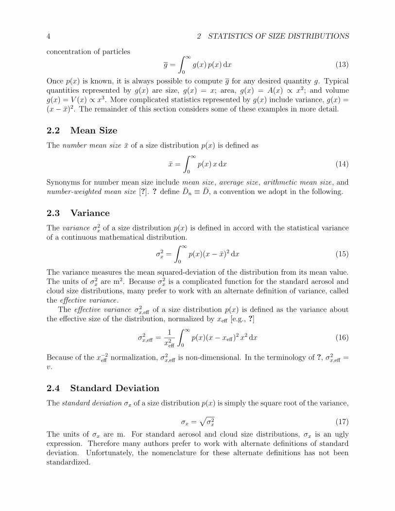
Once p(x) is known, it is always possible to compute g for any desired quantity g. Typicalquantities represented by g(x) are size, g(x) = x; area, g(x) = A(x) ∝ x2; and volumeg(x) = V (x) ∝ x3. More complicated statistics represented by g(x) include variance, g(x) =(x − x)2. The remainder of this section considers some of these examples in more detail.
2.2 Mean Size
The number mean size x of a size distribution p(x) is defined as
x =
∫ ∞
0
p(x) x dx (14)
Synonyms for number mean size include mean size, average size, arithmetic mean size, andnumber-weighted mean size [?]. ? define Dn ≡ D, a convention we adopt in the following.
2.3 Variance
The variance σ2x of a size distribution p(x) is defined in accord with the statistical variance
of a continuous mathematical distribution.
σ2x =
∫ ∞
0
p(x)(x − x)2 dx (15)
The variance measures the mean squared-deviation of the distribution from its mean value.The units of σ2
x are m2. Because σ2x is a complicated function for the standard aerosol and
cloud size distributions, many prefer to work with an alternate definition of variance, calledthe effective variance.
The effective variance σ2x,eff of a size distribution p(x) is defined as the variance about
the effective size of the distribution, normalized by xeff [e.g., ?]
σ2x,eff =
1
x2eff
∫ ∞
0
p(x)(x − xeff)2 x2 dx (16)
Because of the x−2eff normalization, σ2
x,eff is non-dimensional. In the terminology of ?, σ2x,eff =
v.
2.4 Standard Deviation
The standard deviation σx of a size distribution p(x) is simply the square root of the variance,
σx =√
σ2x (17)
The units of σx are m. For standard aerosol and cloud size distributions, σx is an uglyexpression. Therefore many authors prefer to work with alternate definitions of standarddeviation. Unfortunately, the nomenclature for these alternate definitions has not beenstandardized.
5
3 Cloud and Aerosol Size Distributions
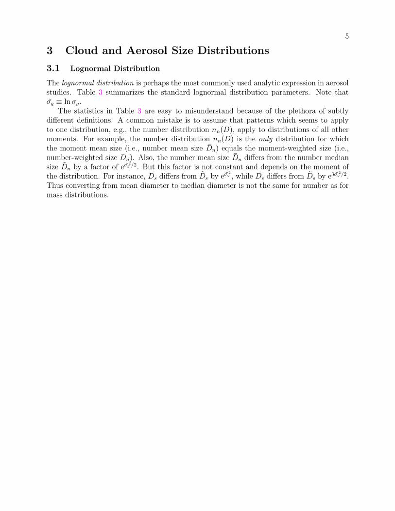
3.1 Lognormal Distribution
The lognormal distribution is perhaps the most commonly used analytic expression in aerosolstudies. Table 3 summarizes the standard lognormal distribution parameters. Note thatσg ≡ ln σg.
The statistics in Table 3 are easy to misunderstand because of the plethora of subtlydifferent definitions. A common mistake is to assume that patterns which seems to applyto one distribution, e.g., the number distribution nn(D), apply to distributions of all othermoments. For example, the number distribution nn(D) is the only distribution for whichthe moment mean size (i.e., number mean size Dn) equals the moment-weighted size (i.e.,number-weighted size Dn). Also, the number mean size Dn differs from the number mediansize Dn by a factor of eσg
2/2. But this factor is not constant and depends on the moment ofthe distribution. For instance, Ds differs from Ds by eσg
2
, while Ds differs from Ds by e3σg2/2.
Thus converting from mean diameter to median diameter is not the same for number as formass distributions.
63
CLO
UD
AN
DA
ER
OSO
LSIZ
ED
IST
RIB
UT
ION
S
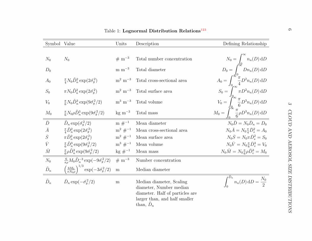
Table 1: Lognormal Distribution Relations123
Symbol Value Units Description Defining Relationship
N0 N0 # m−3 Total number concentration N0 =
∫ ∞
0
nn(D) dD
D0 m m−3 Total diameter D0 =
∫ ∞
0
Dnn(D) dD
A0π4N0D
2n exp(2σg
2) m2 m−3 Total cross-sectional area A0 =
∫ ∞
0
π
4D2nn(D) dD
S0 πN0D2n exp(2σg
2) m2 m−3 Total surface area S0 =
∫ ∞
0
πD2nn(D) dD
V0π6N0D
3n exp(9σg
2/2) m3 m−3 Total volume V0 =
∫ ∞
0
π
6D3nn(D) dD
M0π6N0ρD3
n exp(9σg2/2) kg m−3 Total mass M0 =
∫ ∞
0
π
6ρD3nn(D) dD
D Dn exp(σg2/2) m #−1 Mean diameter N0D = N0Dn = D0
A π4D2
n exp(2σg2) m2 #−1 Mean cross-sectional area N0A = N0
π4D2
s = A0
S πD2n exp(2σg
2) m2 #−1 Mean surface area N0S = N0πD2s = S0
V π6D3
n exp(9σg2/2) m3 #−1 Mean volume N0V = N0
π6D3
v = V0
M π6ρD3
n exp(9σg2/2) kg #−1 Mean mass N0M = N0
π6ρD3
v = M0
N06πρ
M0D−3n exp(−9σg
2/2) # m−3 Number concentration
Dn
(
6M0
πN0ρ
)1/3
exp(−3σg2/2) m Median diameter
Dn Dn exp(−σg2/2) m Median diameter, Scaling
diameter, Number mediandiameter. Half of particles arelarger than, and half smallerthan, Dn
∫ Dn
0
nn(D) dD =N0
2

3.1
Lognorm
alD
istributio
n7
Table 1: (continued)
Symbol Value Units Description Defining Relationship
Dn,D, Dn
Dn exp(σg2/2) m Mean diameter, Average
diameter, Number-weightedmean diameter
Dn =1
N0
∫ ∞
0
Dnn(D) dD
Ds Dn exp(σg2) m Surface mean diameter N0πD2
s = N0S = S0
Dv Dn exp(3σg2/2) m Volume mean diameter, Mass
mean diameterN0
π
6D3
v = N0V = V0
Ds Dn exp(2σg2) m Surface median diameter
∫ Ds
0
πD2nn(D) dD =S0
2
Ds,Deff
Dn exp(5σg2/2) m Area-weighted mean diameter,
effective diameterDx =
1
A0
∫ ∞
0
Dπ
4D2nn(D) dD
Dv Dn exp(3σg2) m Volume median diameter
Mass median diameter
∫ Dv
0
π
6D3nn(D) dD =
V0
2
Dv Dn exp(7σg2/2) m Mass-weighted mean diameter,
Volume-weighted meandiameter
Dv =1
V0
∫ ∞
0
Dπ
6D3nn(D) dD

8 3 CLOUD AND AEROSOL SIZE DISTRIBUTIONS
Table 2 lists applies the relations in Table 3 to specific size distributions typical of tropo-spheric aerosols. ? and ? describe measurements and transport of dust across the Atlanticand Pacific, respectively. ? summarize historical measurements of dust size distributions,and analyze the influence of measurement technique on the derived size distribution. Theyshow the derived size distribution is strongly sensitive to the measurment technique. DuringPRIDE, measured Dv varied from 2.5–9 µm depending on the instrument employed. ? showthat the change in mineral dust size distribution across the sub-tropical Atlantic is consistentwith a slight updraft of ∼ 0.33 cm s−1 during transport. ? and ? show that the effectsof asphericity on particle settling velocity play an important role in maintaining the largeparticle tail of the size distribution during long range transport.
Table 3 applies the relations in Table 3 to specific size distributions typical of troposphericaerosols.
3.1.1 Distribution Function
The lognormal distribution function is
nn(D) =1√
2π D ln σg
exp
−1
2
(
ln(D/Dn)
ln σg
)2
(18)
One of the most confusing aspects of size distributions in the meteorological literature is inthe usage of σg, which is frequently called the geometric standard deviation. Some researchers[e.g., ?] denote by σg what most denote by ln σg. Thus the form of the lognormal distributionfunction sometimes appears
nn(D) =1√
2π σgDexp
−1
2
(
ln(D/Dn)
σg
)2
(19)
In practice, (18) is used more widely than (19) but the definition of σg in the latter may bemore satisfactory from a mathematical point of view [?] (and it subsumes the “ln”, whichreduces typing). We adopt (18) in the following, and sometimes simplify formulae by usinga convenient definition of σg ≡ ln σg. One is occasionally given a “standard deviation” or“geometric standard deviation” parameter without clear specification whether it representsσg (or ln σg, or exp σg, or σx) in (17), (18), or (19). A useful rule of thumb is that σg in (18)and eσg in (19) are usually near 2.0 for realistic aerosol populations. Since we adopted (18),physically realistic values of σg presented in this manuscript will be near 2.0.
Note that direct substitution of D = 2r into (18) yields
nn(D) =1√
2π 2r ln σg
exp
[
−1
2
(
ln(2r/2rn)
ln σg
)2]
=1
2
1√2π r ln σg
exp
[
−1
2
(
ln(r/rn)
ln σg
)2]
=1
2nr
n(r) (20)
in agreement with (12).

3.1 Lognormal Distribution 9
Table 2: Lognormal Size Distribution Statistics
Dn Dv σg M Ref.a
µm µm
?b
0.003291 0.0111 1.89 2.6 × 10⁻⁴ 2
0.5972 2.524 2.0c 0.781 2, 4
7.575 42.1 2.13 0.219 2
?d
0.1600 0.832 2.1 0.036 3
1.401 4.82 1.90 0.957 3
9.989 19.38 1.60 0.007 3
? e
0.08169 0.27 1.88 1
0.8674 5.6 2.2 1
28.65 57.6 1.62 1
aReferences: 1, ?; 2, ?; 3, ?; 4, ?. Values reported in literature were converted to values shown in tableusing the analytic expressions summarized in Table 3. Usually this entailed deriving Dn given Dv, rv, orDs.
bBackground Desert Model from ?, p. 75 Table 1.cσg = 2.0 for transport mode follows ?, p. 10581, Table 1.d?, p. 73 Table 2. These are the “background” modes of D’Almeida (1987).
eDetailed fits to dust sampled over Colorado and Texas in ?, p. 2080 Table 1. Original values have beenconverted from radius to diameter. M was not given. ? showed soil aerosol could be represented with threemodes which they dubbed, in order of increasing size, modes C, A, and B. Mode A is the mineral dusttransport mode, seen in source regions and downwind. Mode B is seen in the source soil itself, and in theatmosphere during dust events. Mode C is seen most everywhere, but does not usually correlate with localdust amount. Mode C is usually a global, aged, background, anthropogenic aerosol, typically rich in sulfateand black carbon. Sometimes, however, Mode C has a mineral dust component. Modes C and B are averagesfrom ? Table 1 p. 2080. Mode B is based on the summary recommendation that rs = 1.5 and σg = 2.2.
10 3 CLOUD AND AEROSOL SIZE DISTRIBUTIONS
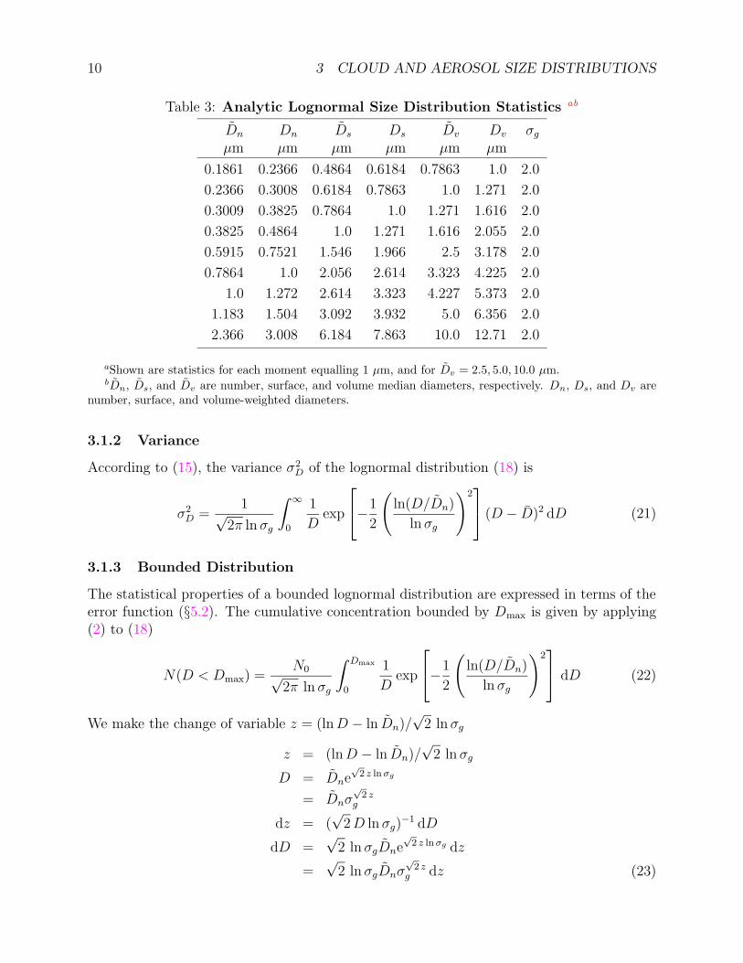
Table 3: Analytic Lognormal Size Distribution Statistics ab
Dn Dn Ds Ds Dv Dv σg
µm µm µm µm µm µm
0.1861 0.2366 0.4864 0.6184 0.7863 1.0 2.0
0.2366 0.3008 0.6184 0.7863 1.0 1.271 2.0
0.3009 0.3825 0.7864 1.0 1.271 1.616 2.0
0.3825 0.4864 1.0 1.271 1.616 2.055 2.0
0.5915 0.7521 1.546 1.966 2.5 3.178 2.0
0.7864 1.0 2.056 2.614 3.323 4.225 2.0
1.0 1.272 2.614 3.323 4.227 5.373 2.0
1.183 1.504 3.092 3.932 5.0 6.356 2.0
2.366 3.008 6.184 7.863 10.0 12.71 2.0
aShown are statistics for each moment equalling 1 µm, and for Dv = 2.5, 5.0, 10.0 µm.bDn, Ds, and Dv are number, surface, and volume median diameters, respectively. Dn, Ds, and Dv are
number, surface, and volume-weighted diameters.
3.1.2 Variance
According to (15), the variance σ2D of the lognormal distribution (18) is
σ2D =
1√2π ln σg
∫ ∞
0
1
Dexp
−1
2
(
ln(D/Dn)
ln σg
)2
(D − D)2 dD (21)
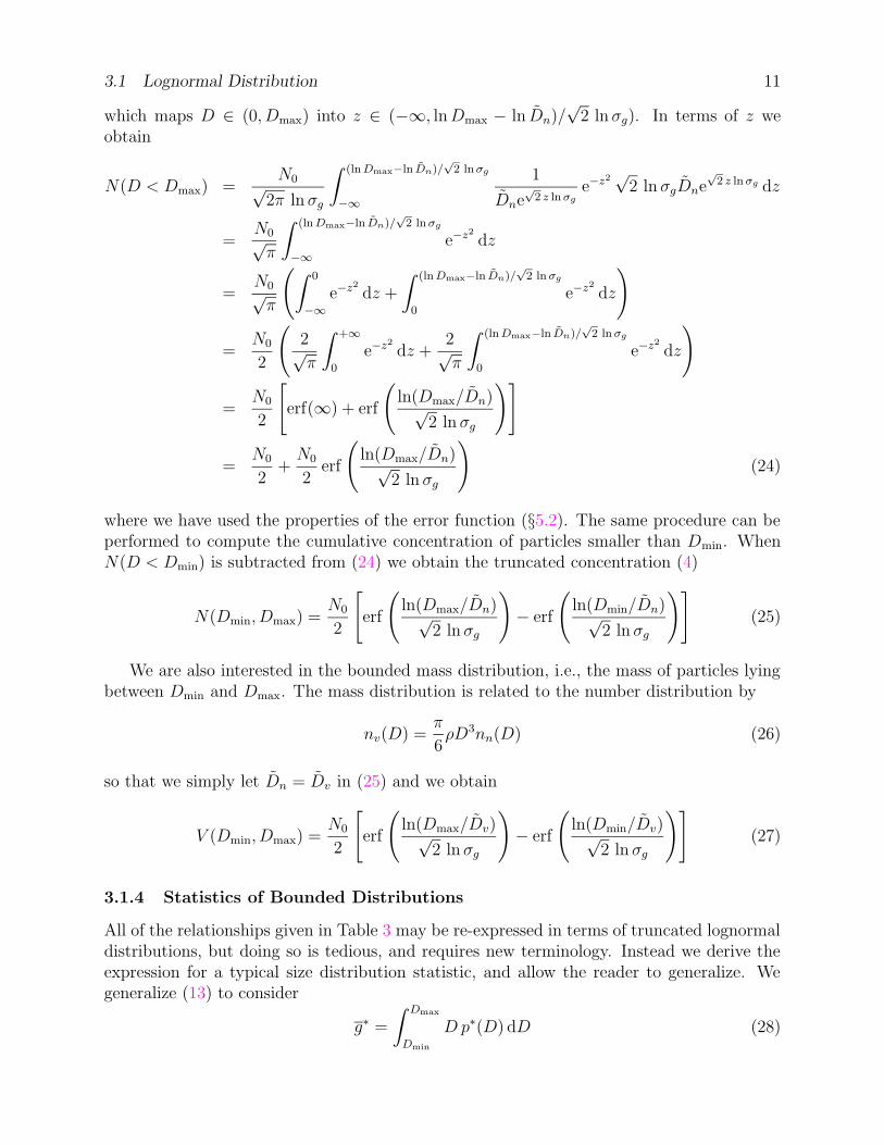
3.1.3 Bounded Distribution
The statistical properties of a bounded lognormal distribution are expressed in terms of theerror function (§5.2). The cumulative concentration bounded by Dmax is given by applying(2) to (18)
N(D < Dmax) =N0√
2π ln σg
∫ Dmax
0
1
Dexp
−1
2
(
ln(D/Dn)
ln σg
)2
dD (22)
We make the change of variable z = (ln D − ln Dn)/√
2 ln σg
z = (ln D − ln Dn)/√
2 ln σg
D = Dne√
2 z ln σg
= Dnσ√
2 zg
dz = (√
2 D ln σg)−1 dD
dD =√
2 ln σgDne√
2 z ln σg dz
=√
2 ln σgDnσ√
2 zg dz (23)
3.1 Lognormal Distribution 11
which maps D ∈ (0, Dmax) into z ∈ (−∞, ln Dmax − ln Dn)/√
2 ln σg). In terms of z weobtain
N(D < Dmax) =N0√
2π ln σg
∫ (ln Dmax−ln Dn)/√
2 ln σg
−∞
1
Dne√
2 z ln σg
e−z2√
2 ln σgDne√
2 z ln σg dz
=N0√
π
∫ (ln Dmax−ln Dn)/√
2 ln σg
−∞
e−z2
dz
=N0√
π
(
∫ 0
−∞
e−z2
dz +
∫ (ln Dmax−ln Dn)/√
2 ln σg
0
e−z2
dz
)
=N0
2
(
2√π
∫ +∞
0
e−z2
dz +2√π
∫ (ln Dmax−ln Dn)/√
2 ln σg
0
e−z2
dz
)
=N0
2
[
erf(∞) + erf
(
ln(Dmax/Dn)√2 ln σg
)]
=N0
2+
N0
2erf
(
ln(Dmax/Dn)√2 ln σg
)
(24)
where we have used the properties of the error function (§5.2). The same procedure can beperformed to compute the cumulative concentration of particles smaller than Dmin. WhenN(D < Dmin) is subtracted from (24) we obtain the truncated concentration (4)
N(Dmin, Dmax) =N0
2
[
erf
(
ln(Dmax/Dn)√2 ln σg
)
− erf
(
ln(Dmin/Dn)√2 ln σg
)]
(25)
We are also interested in the bounded mass distribution, i.e., the mass of particles lyingbetween Dmin and Dmax. The mass distribution is related to the number distribution by
nv(D) =π
6ρD3nn(D) (26)
so that we simply let Dn = Dv in (25) and we obtain
V (Dmin, Dmax) =N0
2
[
erf
(
ln(Dmax/Dv)√2 ln σg
)
− erf
(
ln(Dmin/Dv)√2 ln σg
)]
(27)
3.1.4 Statistics of Bounded Distributions
All of the relationships given in Table 3 may be re-expressed in terms of truncated lognormaldistributions, but doing so is tedious, and requires new terminology. Instead we derive theexpression for a typical size distribution statistic, and allow the reader to generalize. Wegeneralize (13) to consider
g∗ =
∫ Dmax
Dmin
D p∗(D) dD (28)
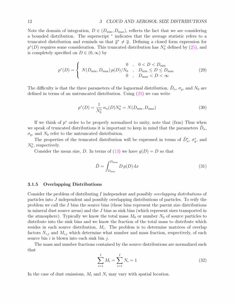
12 3 CLOUD AND AEROSOL SIZE DISTRIBUTIONS
Note the domain of integration, D ∈ (Dmin, Dmax), reflects the fact that we are consideringa bounded distribution. The superscript ∗ indicates that the average statistic refers to atruncated distribution and reminds us that g∗ 6= g. Defining a closed form expression forp∗(D) requires some consideration. This truncated distribution has N ∗
0 defined by (25), andis completely specified on D ∈ (0,∞) by
p∗(D) =
0 , 0 < D < Dmin
N(Dmin, Dmax) p(D)/N0 , Dmin ≤ D ≤ Dmax
0 , Dmax < D < ∞(29)
The difficulty is that the three parameters of the lognormal distribution, Dn, σg, and N0 aredefined in terms of an untruncated distribution. Using (25) we can write
p∗(D) =1
N∗0
nn(D)N ∗0 = N(Dmin, Dmax) (30)
If we think of p∗ order to be properly normalized to unity, note that (fxm) Thus whenwe speak of truncated distributions it is important to keep in mind that the parameters Dn,σg, and N0 refer to the untruncated distribution.
The properties of the truncated distribution will be expressed in terms of D∗n, σ∗
g , andN∗
0 , respectively.
Consider the mean size, D. In terms of (13) we have g(D) = D so that
D =
∫ Dmax
Dmin
D p(D) dx (31)
3.1.5 Overlapping Distributions
Consider the problem of distributing I independent and possibly overlapping distributions ofparticles into J independent and possibly overlapping distributions of particles. To reify theproblem we call the I bins the source bins (these bins represent the parent size distributionsin mineral dust source areas) and the J bins as sink bins (which represent sizes transported inthe atmosphere). Typically we know the total mass M0 or number N0 of source particles todistribute into the sink bins and we know the fraction of the total mass to distribute whichresides in each source distribution, Mi. The problem is to determine matrices of overlapfactors Ni,j and Mi,j which determine what number and mass fraction, respectively, of eachsource bin i is blown into each sink bin j.
The mass and number fractions contained by the source distributions are normalized suchthat
I∑
i=1
Mi =I∑
i=1
Ni = 1 (32)
In the case of dust emissions, Mi and Ni may vary with spatial location.
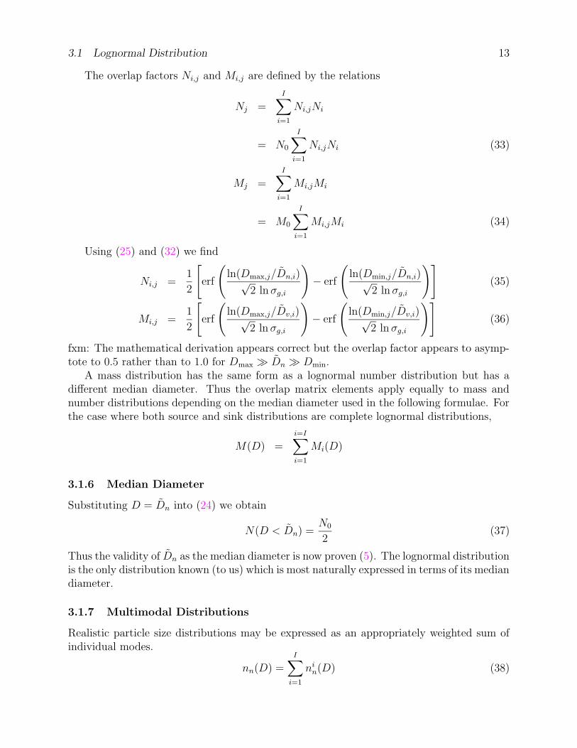
3.1 Lognormal Distribution 13
The overlap factors Ni,j and Mi,j are defined by the relations
Nj =I∑
i=1
Ni,jNi
= N0
I∑
i=1
Ni,jNi (33)
Mj =I∑
i=1
Mi,jMi
= M0
I∑
i=1
Mi,jMi (34)
Using (25) and (32) we find
Ni,j =1
2
[
erf
(
ln(Dmax,j/Dn,i)√2 ln σg,i
)
− erf
(
ln(Dmin,j/Dn,i)√2 ln σg,i
)]
(35)
Mi,j =1
2
[
erf
(
ln(Dmax,j/Dv,i)√2 ln σg,i
)
− erf
(
ln(Dmin,j/Dv,i)√2 ln σg,i
)]
(36)
fxm: The mathematical derivation appears correct but the overlap factor appears to asymp-tote to 0.5 rather than to 1.0 for Dmax � Dn � Dmin.
A mass distribution has the same form as a lognormal number distribution but has adifferent median diameter. Thus the overlap matrix elements apply equally to mass andnumber distributions depending on the median diameter used in the following formulae. Forthe case where both source and sink distributions are complete lognormal distributions,
M(D) =i=I∑
i=1
Mi(D)
3.1.6 Median Diameter
Substituting D = Dn into (24) we obtain
N(D < Dn) =N0
2(37)
Thus the validity of Dn as the median diameter is now proven (5). The lognormal distributionis the only distribution known (to us) which is most naturally expressed in terms of its mediandiameter.
3.1.7 Multimodal Distributions
Realistic particle size distributions may be expressed as an appropriately weighted sum ofindividual modes.
nn(D) =I∑
i=1
nin(D) (38)
14 3 CLOUD AND AEROSOL SIZE DISTRIBUTIONS
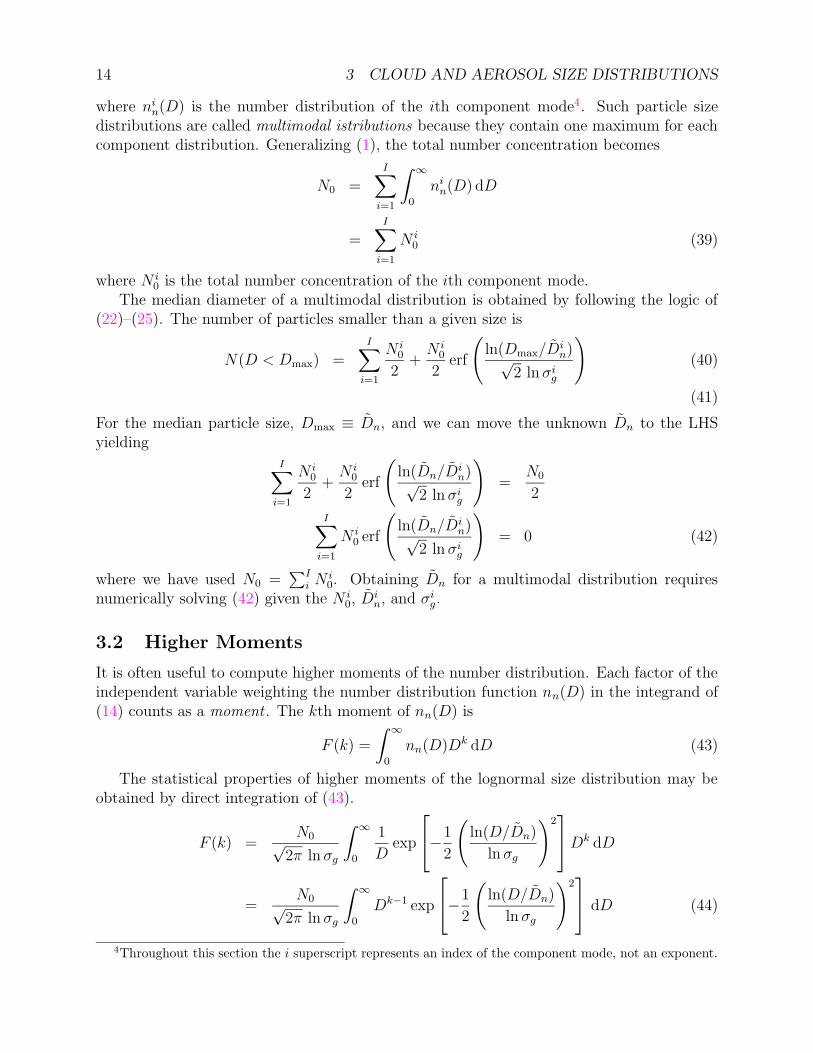
where nin(D) is the number distribution of the ith component mode4. Such particle size
distributions are called multimodal istributions because they contain one maximum for eachcomponent distribution. Generalizing (1), the total number concentration becomes
N0 =I∑
i=1
∫ ∞
0
nin(D) dD
=I∑
i=1
N i0 (39)
where N i0 is the total number concentration of the ith component mode.
The median diameter of a multimodal distribution is obtained by following the logic of(22)–(25). The number of particles smaller than a given size is
N(D < Dmax) =I∑
i=1
N i0
2+
N i0
2erf
(
ln(Dmax/Din)√
2 ln σig
)
(40)
(41)
For the median particle size, Dmax ≡ Dn, and we can move the unknown Dn to the LHSyielding
I∑
i=1
N i0
2+
N i0
2erf
(
ln(Dn/Din)√
2 ln σig
)
=N0
2
I∑
i=1
N i0 erf
(
ln(Dn/Din)√
2 ln σig
)
= 0 (42)
where we have used N0 =∑I
i N i0. Obtaining Dn for a multimodal distribution requires
numerically solving (42) given the N i0, Di
n, and σig.
3.2 Higher Moments
It is often useful to compute higher moments of the number distribution. Each factor of theindependent variable weighting the number distribution function nn(D) in the integrand of(14) counts as a moment . The kth moment of nn(D) is
F (k) =
∫ ∞
0
nn(D)Dk dD (43)
The statistical properties of higher moments of the lognormal size distribution may beobtained by direct integration of (43).
F (k) =N0√
2π ln σg
∫ ∞
0
1
Dexp
−1
2
(
ln(D/Dn)
ln σg
)2
Dk dD
=N0√
2π ln σg
∫ ∞
0
Dk−1 exp
−1
2
(
ln(D/Dn)
ln σg
)2
dD (44)
4Throughout this section the i superscript represents an index of the component mode, not an exponent.
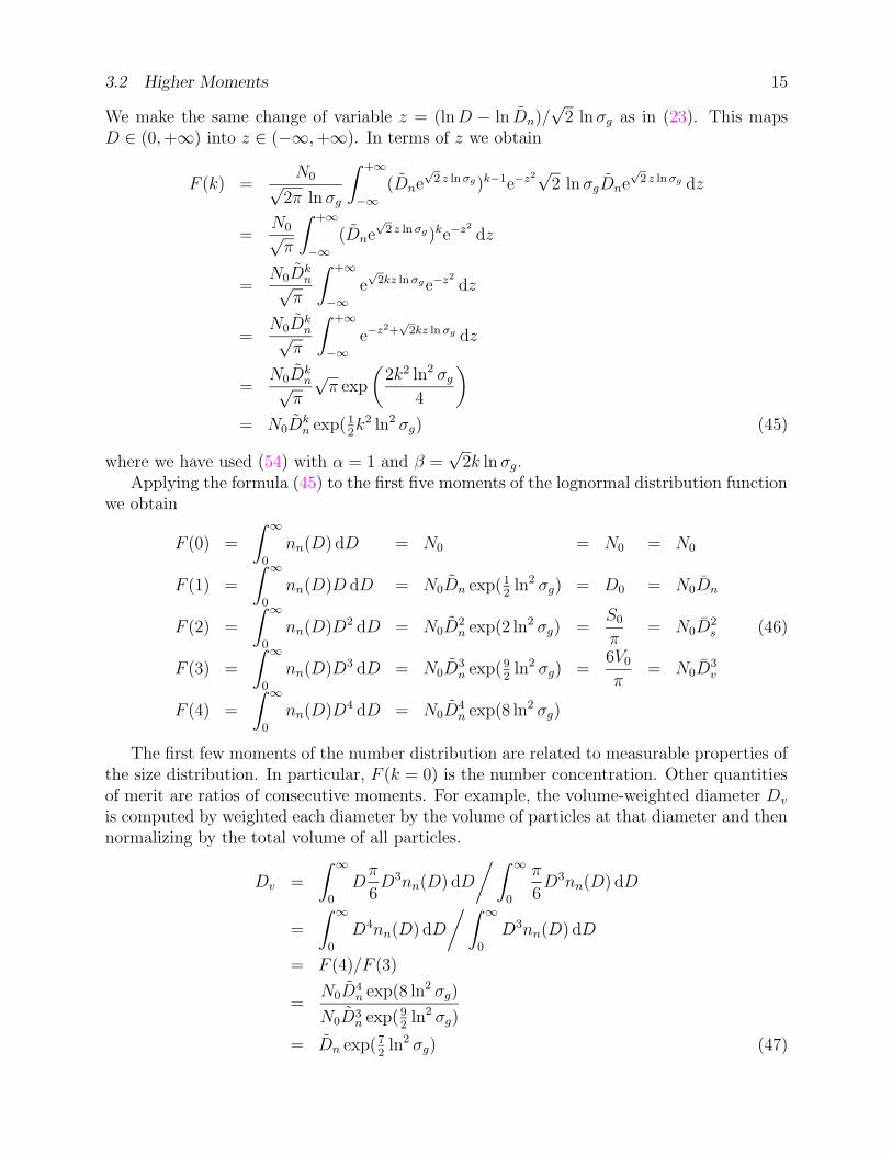
3.2 Higher Moments 15
We make the same change of variable z = (ln D − ln Dn)/√
2 ln σg as in (23). This mapsD ∈ (0, +∞) into z ∈ (−∞, +∞). In terms of z we obtain
F (k) =N0√
2π ln σg
∫ +∞
−∞
(Dne√
2 z ln σg)k−1e−z2√
2 ln σgDne√
2 z ln σg dz
=N0√
π
∫ +∞
−∞
(Dne√
2 z ln σg)ke−z2
dz
=N0D
kn√
π
∫ +∞
−∞
e√
2kz ln σge−z2
dz
=N0D
kn√
π
∫ +∞
−∞
e−z2+√
2kz ln σg dz
=N0D
kn√
π
√π exp
(
2k2 ln2 σg
4
)
= N0Dkn exp(1
2k2 ln2 σg) (45)
where we have used (54) with α = 1 and β =√
2k ln σg.Applying the formula (45) to the first five moments of the lognormal distribution function
we obtain
F (0) =
∫ ∞
0
nn(D) dD = N0 = N0 = N0
F (1) =
∫ ∞
0
nn(D)D dD = N0Dn exp(12ln2 σg) = D0 = N0Dn
F (2) =
∫ ∞
0
nn(D)D2 dD = N0D2n exp(2 ln2 σg) =
S0
π= N0D
2s
F (3) =
∫ ∞
0
nn(D)D3 dD = N0D3n exp(9
2ln2 σg) =
6V0
π= N0D
3v
F (4) =
∫ ∞
0
nn(D)D4 dD = N0D4n exp(8 ln2 σg)
(46)
The first few moments of the number distribution are related to measurable properties ofthe size distribution. In particular, F (k = 0) is the number concentration. Other quantitiesof merit are ratios of consecutive moments. For example, the volume-weighted diameter Dv
is computed by weighted each diameter by the volume of particles at that diameter and thennormalizing by the total volume of all particles.
Dv =
∫ ∞
0
Dπ
6D3nn(D) dD
/∫ ∞
0
π
6D3nn(D) dD
=
∫ ∞
0
D4nn(D) dD
/∫ ∞
0
D3nn(D) dD
= F (4)/F (3)
=N0D
4n exp(8 ln2 σg)
N0D3n exp(9
2ln2 σg)
= Dn exp(72ln2 σg) (47)
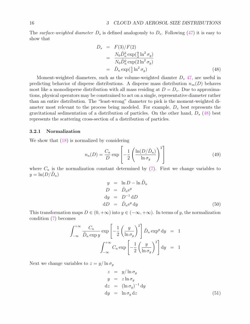
16 3 CLOUD AND AEROSOL SIZE DISTRIBUTIONS
The surface-weighted diameter Ds is defined analogously to Dv. Following (47) it is easy toshow that
Ds = F (3)/F (2)
=N0D
3n exp(9
2ln2 σg)
N0D2n exp(2 ln2 σg)
= Dn exp(52ln2 σg) (48)
Moment-weighted diameters, such as the volume-weighted diamter Dv 47, are useful inpredicting behavior of disperse distributions. A disperse mass distribution nm(D) behavesmost like a monodisperse distribution with all mass residing at D = Dv. Due to approxima-tions, physical operators may be constrained to act on a single, representative diameter ratherthan an entire distribution. The “least-wrong” diameter to pick is the moment-weighted di-ameter most relevant to the process being modeled. For example, Dv best represents thegravitational sedimentation of a distribution of particles. On the other hand, Ds (48) bestrepresents the scattering cross-section of a distribution of particles.
3.2.1 Normalization
We show that (18) is normalized by considering
nn(D) =Cn
Dexp
−1
2
(
ln(D/Dn)
ln σg
)2
(49)
where Cn is the normalization constant determined by (7). First we change variables toy = ln(D/Dn)
y = ln D − ln Dn
D = Dney
dy = D−1 dD
dD = Dney dy (50)
This transformation maps D ∈ (0, +∞) into y ∈ (−∞, +∞). In terms of y, the normalizationcondition (7) becomes
∫ +∞
−∞
Cn
Dn exp yexp
[
−1
2
(
y
ln σg
)2]
Dn expy dy = 1
∫ +∞
−∞
Cn exp
[
−1
2
(
y
ln σg
)2]
dy = 1
Next we change variables to z = y/ ln σg
z = y/ ln σg
y = z ln σg
dz = (ln σg)−1 dy
dy = ln σg dz (51)

17
Soil Texture Dn σg Description
Sand Sand
Silt Silt
Clay Clay
Soil Texture Dn σg DescriptionSand Sand
Silt Silt
Clay Clay
Table 4: Source size distribution associated with surface soil texture data of ? and of ?.
This transformation does not change the limits of integration and we obtain
∫ +∞
−∞
Cn exp
(−z2
2
)
ln σg dz = 1
Cn
√2π ln σg = 1
Cn =1√
2π ln σg
(52)
In the above we used the well-known normalization property of the Gaussian distributionfunction,
∫ +∞
−∞e−x2/2 dx =
√2π (53).
4 Implementation in NCAR models
The discussion thus far has centered on the theoretical considerations of size distributions.In practice, these ideas must be implemented in computer codes which model, e.g., Mie scat-tering parameters or thermodynamic growth of aerosol populations. This section describeshow these ideas have been implemented in the NCAR-Dust and Mie models.
4.1 NCAR-Dust Model
The NCAR-Dust model uses as input a time invariant dataset of surface soil size distribution.The two such datasets currently used are from ? and from IBIS [?]. The ? dataset providesglobal information for three soil texture types: sand, clay and silt. At each gridpoint, themass flux of dust is partitioned into mass contributions from each of these soil types. Toaccomplish this, the partitioning scheme assumes a size distribution for the source soil of thedeflated particles. Table 4 lists the lognormal distribution parameters associated with thesurface soil texture data of ? and of ?. The dust model is a size resolving aerosol model.Thus, overlap factors are computed to determine the fraction of each parent size type whichis mobilized into each atmospheric dust size bin during a deflation event.
18 4 IMPLEMENTATION IN NCAR MODELS
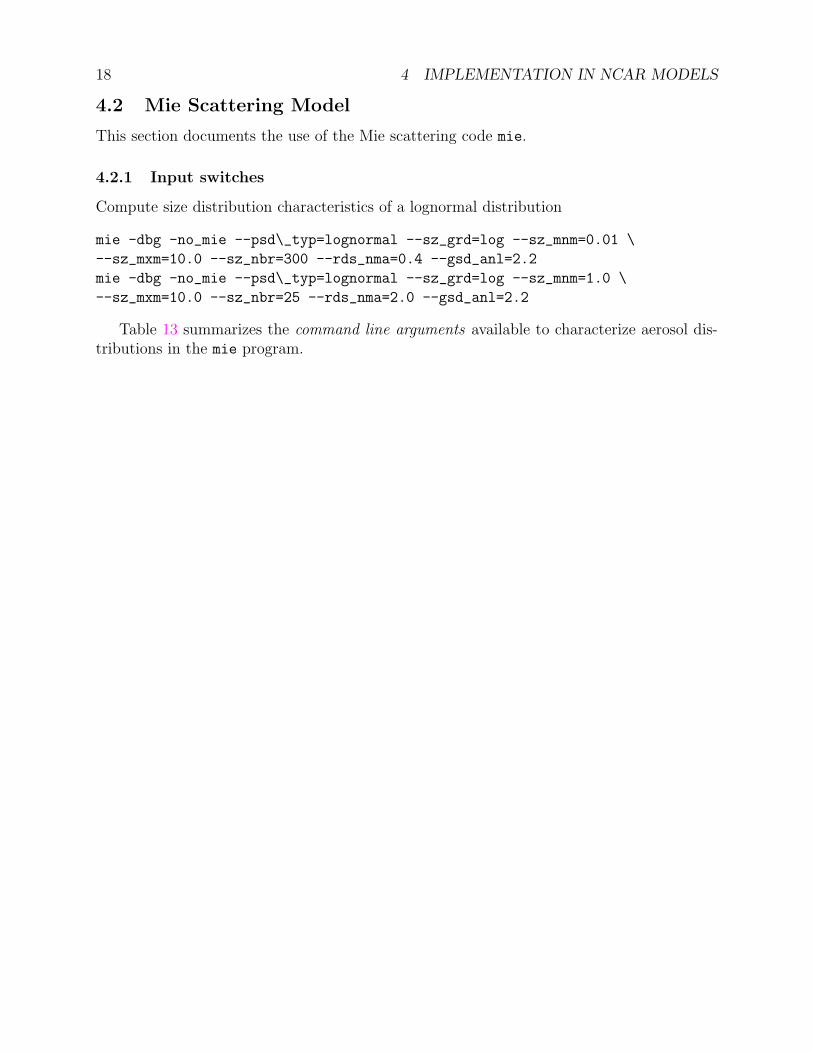
4.2 Mie Scattering Model
This section documents the use of the Mie scattering code mie.
4.2.1 Input switches
Compute size distribution characteristics of a lognormal distribution
mie -dbg -no_mie --psd\_typ=lognormal --sz_grd=log --sz_mnm=0.01 \
--sz_mxm=10.0 --sz_nbr=300 --rds_nma=0.4 --gsd_anl=2.2
mie -dbg -no_mie --psd\_typ=lognormal --sz_grd=log --sz_mnm=1.0 \
--sz_mxm=10.0 --sz_nbr=25 --rds_nma=2.0 --gsd_anl=2.2
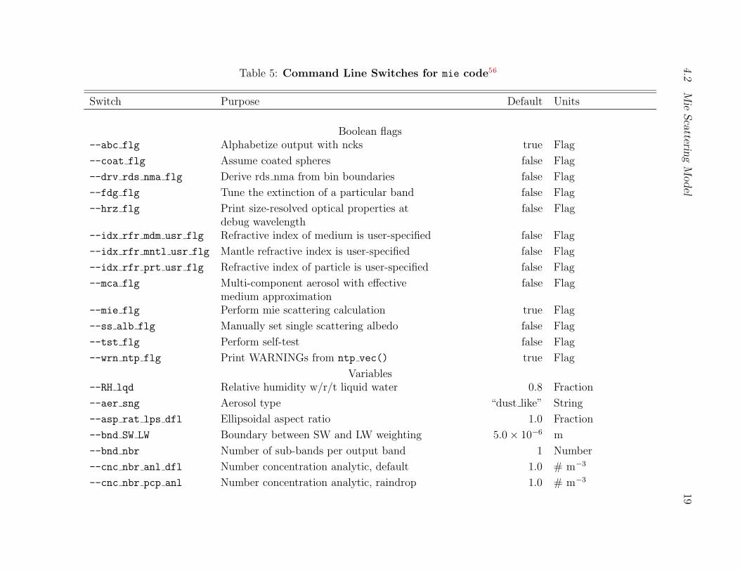
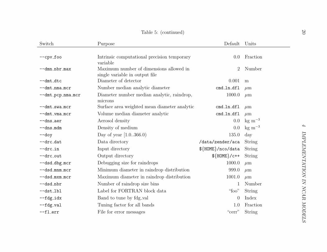
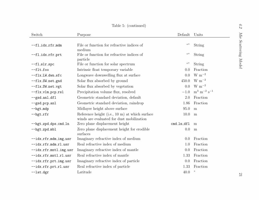
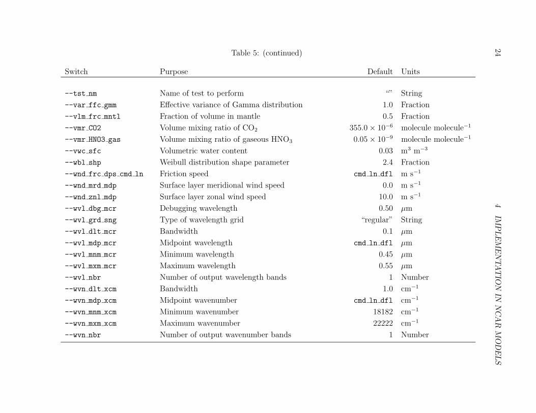
Table 13 summarizes the command line arguments available to characterize aerosol dis-tributions in the mie program.
4.2
Mie
Sca
ttering
Model
19
Table 5: Command Line Switches for mie code56
Switch Purpose Default Units
Boolean flags--abc flg Alphabetize output with ncks true Flag
--coat flg Assume coated spheres false Flag
--drv rds nma flg Derive rds nma from bin boundaries false Flag
--fdg flg Tune the extinction of a particular band false Flag
--hrz flg Print size-resolved optical properties atdebug wavelength
false Flag
--idx rfr mdm usr flg Refractive index of medium is user-specified false Flag
--idx rfr mntl usr flg Mantle refractive index is user-specified false Flag
--idx rfr prt usr flg Refractive index of particle is user-specified false Flag
--mca flg Multi-component aerosol with effectivemedium approximation
false Flag
--mie flg Perform mie scattering calculation true Flag
--ss alb flg Manually set single scattering albedo false Flag
--tst flg Perform self-test false Flag
--wrn ntp flg Print WARNINGs from ntp vec() true Flag
Variables--RH lqd Relative humidity w/r/t liquid water 0.8 Fraction
--aer sng Aerosol type “dust like” String
--asp rat lps dfl Ellipsoidal aspect ratio 1.0 Fraction
--bnd SW LW Boundary between SW and LW weighting 5.0 × 10⁻⁶ m
--bnd nbr Number of sub-bands per output band 1 Number
--cnc nbr anl dfl Number concentration analytic, default 1.0 # m−3
--cnc nbr pcp anl Number concentration analytic, raindrop 1.0 # m−3
204
IMP
LE
ME
NTAT
ION
INN
CA
RM
OD
ELS
Table 5: (continued)
Switch Purpose Default Units
--cpv foo Intrinsic computational precision temporaryvariable
0.0 Fraction
--dmn nbr max Maximum number of dimensions allowed insingle variable in output file
2 Number
--dmt dtc Diameter of detector 0.001 m
--dmt nma mcr Number median analytic diameter cmd ln dfl µm
--dmt pcp nma mcr Diameter number median analytic, raindrop,microns
1000.0 µm
--dmt swa mcr Surface area weighted mean diameter analytic cmd ln dfl µm
--dmt vma mcr Volume median diameter analytic cmd ln dfl µm
--dns aer Aerosol density 0.0 kg m−3
--dns mdm Density of medium 0.0 kg m−3
--doy Day of year [1.0..366.0) 135.0 day
--drc dat Data directory /data/zender/aca String
--drc in Input directory ${HOME}/nco/data String
--drc out Output directory ${HOME}/c++ String
--dsd dbg mcr Debugging size for raindrops 1000.0 µm
--dsd mnm mcr Minimum diameter in raindrop distribution 999.0 µm
--dsd mxm mcr Maximum diameter in raindrop distribution 1001.0 µm
--dsd nbr Number of raindrop size bins 1 Number
--dst lbl Label for FORTRAN block data “foo” String
--fdg idx Band to tune by fdg val 0 Index
--fdg val Tuning factor for all bands 1.0 Fraction
--fl err File for error messages “cerr” String
4.2
Mie
Sca
ttering
Model
21
Table 5: (continued)
Switch Purpose Default Units
--fl idx rfr mdm File or function for refractive indices ofmedium
“” String
--fl idx rfr prt File or function for refractive indices ofparticle
“” String
--fl slr spc File or function for solar spectrum “” String
--flt foo Intrinsic float temporary variable 0.0 Fraction
--flx LW dwn sfc Longwave downwelling flux at surface 0.0 W m−2
--flx SW net gnd Solar flux absorbed by ground 450.0 W m−2
--flx SW net vgt Solar flux absorbed by vegetation 0.0 W m−2
--flx vlm pcp rsl Precipitation volume flux, resolved −1.0 m3 m−2 s−1
--gsd anl dfl Geometric standard deviation, default 2.0 Fraction
--gsd pcp anl Geometric standard deviation, raindrop 1.86 Fraction
--hgt mdp Midlayer height above surface 95.0 m
--hgt rfr Reference height (i.e., 10 m) at which surfacewinds are evaluated for dust mobilization
10.0 m
--hgt zpd dps cmd ln Zero plane displacement height cmd ln dfl m
--hgt zpd mbl Zero plane displacement height for erodiblesurfaces
0.0 m
--idx rfr mdm img usr Imaginary refractive index of medium 0.0 Fraction
--idx rfr mdm rl usr Real refractive index of medium 1.0 Fraction
--idx rfr mntl img usr Imaginary refractive index of mantle 0.0 Fraction
--idx rfr mntl rl usr Real refractive index of mantle 1.33 Fraction
--idx rfr prt img usr Imaginary refractive index of particle 0.0 Fraction
--idx rfr prt rl usr Real refractive index of particle 1.33 Fraction
--lat dgr Latitude 40.0 ◦

224
IMP
LE
ME
NTAT
ION
INN
CA
RM
OD
ELS
Table 5: (continued)
Switch Purpose Default Units
--lbl sng Line-by-line test “CO2” String
--lgn nbr Number of terms in Legendre expansion ofphase function
8 Number
--lnd frc dry Dry land fraction 1.0 Fraction
--mdm sng Medium type “air” String
--mmw aer Mean molecular weight 0.0 kg mol−1
--mno lng dps cmd ln Monin-Obukhov length cmd ln dfl m
--mss frc cly Mass fraction clay 0.19 Fraction
--mss frc snd Mass fraction sand 0.777 Fraction
--ngl nbr Number of angles in Mie computation 11 Number
--oro Orography: ocean=0.0, land=1.0, sea ice=2.0 1.0 Fraction
--pnt typ idx Plant type index 14 Index
--prs mdp Environmental pressure 100825.0 Pa
--prs ntf Environmental surface pressure prs STP Pa
--psd typ Particle size distribution type “lognormal” String
--q H2O vpr Specific humidity cmd ln dfl kg kg−1
--rds ffc gmm mcr Effective radius of Gamma distribution 50.0 µm
--rds nma mcr Number median analytic radius 0.2986 µm
--rds swa mcr Surface area weighted mean radius analytic cmd ln dfl µm
--rds vma mcr Volume median radius analytic cmd ln dfl µm
--rgh mmn dps cmd ln Roughness length momentum cmd ln dfl m
--rgh mmn ice std Roughness length over sea ice 0.0005 m
--rgh mmn mbl Roughness length momentum for erodiblesurfaces
100.0 × 10⁻⁶ m

4.2
Mie
Sca
ttering
Model
23
Table 5: (continued)
Switch Purpose Default Units
--rgh mmn smt Smooth roughness length 10.0 × 10⁻⁶ m
--sfc typ LSM surface type (0..28) 2 Index
--slr cst Solar constant 1367.0 W m−2
--slr spc key Solar spectrum string “LaN68” String
--slr zen ngl cos Cosine solar zenith angle 1.0 Fraction
--snw hgt lqd Equivalent liquid water snow depth 0.0 m
--soi typ LSM soil type (1..5) 1 Index
--spc heat aer Specific heat capacity 0.0 J kg−1 K−1
--ss alb cmd ln Single scattering albedo 1.0 Fraction
--sz dbg mcr Debugging size 1.0 µm
--sz grd sng Type of size grid “logarithmic” String
--sz mnm mcr Minimum size in distribution 0.9 µm
--sz mxm mcr Maximum size in distribution 1.1 µm
--sz nbr Number of particle size bins 1 Number
--sz prm rsn Size parameter resolution 0.1 Fraction
--tm dlt Timestep 1200.0 s
--tpt bbd wgt Blackbody temperature of radiation 273.15 K
--tpt gnd Ground temperature 300.0 K
--tpt ice Ice temperature tpt frz pnt K
--tpt mdp Environmental temperature 300.0 K
--tpt prt Particle temperature 273.15 K
--tpt soi Soil temperature 297.0 K
--tpt sst Sea surface temperature 300.0 K
--tpt vgt Vegetation temperature 300.0 K
244
IMP
LE
ME
NTAT
ION
INN
CA
RM
OD
ELS
Table 5: (continued)
Switch Purpose Default Units
--tst nm Name of test to perform “” String
--var ffc gmm Effective variance of Gamma distribution 1.0 Fraction
--vlm frc mntl Fraction of volume in mantle 0.5 Fraction
--vmr CO2 Volume mixing ratio of CO2 355.0 × 10⁻⁶ molecule molecule−1
--vmr HNO3 gas Volume mixing ratio of gaseous HNO3 0.05 × 10⁻⁹ molecule molecule−1
--vwc sfc Volumetric water content 0.03 m3 m−3
--wbl shp Weibull distribution shape parameter 2.4 Fraction
--wnd frc dps cmd ln Friction speed cmd ln dfl m s−1
--wnd mrd mdp Surface layer meridional wind speed 0.0 m s−1
--wnd znl mdp Surface layer zonal wind speed 10.0 m s−1
--wvl dbg mcr Debugging wavelength 0.50 µm
--wvl grd sng Type of wavelength grid “regular” String
--wvl dlt mcr Bandwidth 0.1 µm
--wvl mdp mcr Midpoint wavelength cmd ln dfl µm
--wvl mnm mcr Minimum wavelength 0.45 µm
--wvl mxm mcr Maximum wavelength 0.55 µm
--wvl nbr Number of output wavelength bands 1 Number
--wvn dlt xcm Bandwidth 1.0 cm−1
--wvn mdp xcm Midpoint wavenumber cmd ln dfl cm−1
--wvn mnm xcm Minimum wavenumber 18182 cm−1
--wvn mxm xcm Maximum wavenumber 22222 cm−1
--wvn nbr Number of output wavenumber bands 1 Number

25
5 Appendix
5.1 Properties of Gaussians
The area under a Gaussian distribution may be expressed analytically when the domain is(−∞, +∞). This result may be obtained (IIRC) by transforming to polar coordinates in thecomplex plane x = r(cos θ + i sin θ).
∫ +∞
−∞
e−x2/2 dx =√
2π (53)
This is a special case of a more general result
∫ +∞
−∞
exp(−αx2 − βx) dx =
√
π
αexp
(
β2
4α
)
where α > 0 (54)
This result may be obtained by completing the square under the integrand, making thechange of variable y = x + β/2α, and applying (53). Substituting α = 1/2 and β = 0 into(54) yields (53).
5.2 Error Function
The error function erf(x) may be defined as the partial integral of a Gaussian curve
erf(z) =2√π
∫ z
0
e−x2
dx (55)
Using (53) and the symmetry of a Gaussian curve, it is simple to show that the errorfunction is bounded by the limits erf(0) = 0 and erf(∞) = 1. Thus erf(z) is the cumulativeprobability function for a normally distributed variable z (???). Most compilers implementerf(x) as an intrinsic function. Thus erf(x) is used to compute areas bounded by finitelognormal distributions (§3.1.3).