spatial macrozoobenthic distribution patterns in relation ...€¦ · spatial macrozoobenthic...

59 (2008) 144–161www.elsevier.com/locate/seares

Journal of Sea Research

Spatial macrozoobenthic distribution patterns in relation to majorenvironmental factors- A case study from the Pomeranian Bay

(southern Baltic Sea)

M. Glockzin, M.L. Zettler ⁎

Department of Biology, Leibniz Institute of Baltic Sea Research (IOW), Seestr. 15, D-18119 Warnemuende, Germany

Received 7 November 2007; received in revised form 18 January 2008; accepted 21 January 2008Available online 8 February 2008

Abstract

The aim of this study was to identify potential environmental “key factors” causing spatial distributions of macrozoobenthiccommunities to improve our understanding concerning benthic biotic/abiotic interactions and ecosystem functioning. To this endbenthic and environmental data, collected over a period of 4 years (2003–2006) at 191 sampling stations in the Pomeranian Bay(southwest Baltic Sea), were analysed. This represents the most comprehensive study performed in this respect in the Baltic Sea upto date and also the necessary first step towards a model able to predict macrofaunal distributions regarding autecological species-environment interactions. Based on species abundances, distinctive macrobenthic community patterns were identified andevaluated via univariate correlation methods, multivariate numerical classification and ordination techniques (e.g. PCA, CCA).These patterns were caused by clear responses of several benthic species to certain prevailing environmental conditions. Theobserved distribution of selected species followed a strong gradient of depth and was explained best by the sediment parameterstotal organic carbon (TOC), median grain size and sorting. By using different statistical methods these abiotic/biotic interactionswere modelled allowing to extend our knowledge concerning ecosystem functioning, and provide a tool to assess natural andanthropogenic forced changes in species distribution.© 2008 Elsevier B.V. All rights reserved.

Keywords: Macrozoobenthos; Environmental factors; Multivariate analysis; PCA; CCA; BIO-ENV; Rank correlation; Pattern analysis; PomeranianBay; Baltic Sea

1. Introduction

Different studies have suggested that substrate com-position, hydrographic parameters and their variationsseem to determine macrofaunal assemblages and abun-dances (e.g. Rumohr et al., 1996; Ellis et al., 2006; Fortin

⁎ Corresponding author. Fax: +49 381 5197440.E-mail address: [email protected]

(M.L. Zettler).

1385-1101/$ - see front matter © 2008 Elsevier B.V. All rights reserved.doi:10.1016/j.seares.2008.01.002

et al., 2005; O'Brien et al., 2003). A link between benthicinfauna distribution and environmental factors has beenassumed but has so far not been established particularlyfor the southwest Baltic Sea. However, to examine andunderstand the structure and dynamics of biotic/environ-mental interactions is of great importance to improve ourknowledge regarding biological and ecological processesnot only in the Baltic; it is mandatory to evaluate naturaland anthropogenic influences and effects on ecologicalsystems (Pavlikakis and Tsihrintzis, 2000). Statistical

mailto:[email protected]

http://dx.doi.org/10.1016/j.seares.2008.01.002

145M. Glockzin, M.L. Zettler / Journal of Sea Research 59 (2008) 144–161

models provide a useful tool to relate ecological featuresto environmental factors and, through validation andmodification, they can reveal the underlying mechanismsresponsible for the structure and organisation of commu-nities (Austin, 1987). However, an exploratory statisticaldescription of the prevailing ecological structure based onobservations always is the indispensible first step(Bourget and Fortin, 1995). The comparison of benthiccommunities normally comprise the analysis of speciesdata obtained from a variety of depths and geographicallocations. That in turn yields the possibility of a limitedexploration of variables, distorted by strong gradients(Bourget et al., 1994) or biased by autocorrelation(Legendre, 1993). Previous benthic studies in thePomeranian Bay and in other regions in a more globalperspective simply have neglected this. The present studyfor the first time takes into account both biotic/environ-mental interactions and the possibility of spatial sideeffects on statistical analyses in the Pomeranian Bay.

Due to the variability of species in terms of habitatselection, reciprocal effects between species’ distribu-tion and environmental factors are manifested inpatterns, visible in their abundances or assemblages(Kolasa and Strayer, 1988; Keitt et al., 2002). Under-standing these patterns requires a two-stage procedure.At first, the patterns in the distribution of the organismsare described and secondly, the parameters causing thisdistribution are determined. Alternatively, patterns inenvironmental variables can be determined first andthen the reactions of organisms to these patterns aredescribed (Legendre and Legendre, 1998). However, inboth cases, in-depth knowledge is needed regarding theautecology of the species for the interpretation of therelationships revealed (Sachs, 1997).

The area investigated in this study, the PomeranianBay, is situated in the southwestern part of the BalticSea. Due to its hydrology and morphology, distinctgradients in environmental variables are present, result-ing in a well-defined division of benthic communities(Kube et al., 1996; Warzocha, 1995). This offers a goodbasis to study biotic/abiotic interactions and to identifythe main environmental factors controlling speciesdistributions. The objectives of the present study wereto (i) relate macozoobenthic data to selected abioticfactors, (ii) test the applicability of univariate and mul-tivariate statistical approaches in order to evaluatespatial distribution patterns of species caused by theirvariability and response toward habitat selection and(iii) undertake a first step towards creating a model toassess species response to natural and anthropogeniceffects on a temporal-spatial scale along environmentalgradients such as in the Baltic Sea.

2. Materials and methods

2.1. Study area

This study was performed in the Pomeranian Bay, arelatively shallow brackish water coastal area in thesouthwestern Baltic Sea. It is situated north of the OderRiver and borders to Germany and Poland. Regardingthe data available, we chose the German part of thePomeranian Bay as the actual area of investigation(Fig. 1). It stretches over 90 km from the Isle of Rügenin the west up to the international border of Poland in theeast. To the south, it borders on the Isle of Usedom(Germany). As northern barrier, the 25 m depth line wasused because it represents a relative “continuous” barrierto the open sea. Likewise, the Greifswalder Bodden Sillfunctioned as a seawards barrier to the southwest.Within these boundaries, the area of the German part ofthe Pomeranian Bay amounts to 3.500 km2. With anaverage depth of about 13 m, its water volume equalsapproximately 46 km3 (dataorigin: this study). Thesubmarine morphology of the Bay is predominantlyshaped by gutters and basins of glacial origin (Neumannand Bublitz, 1968). A large seasonal and thereforepulse-like freshwater discharge of about 17 km3 yr-1

from the Oder River in the south and a steady inflow ofsaltwater from the north results in an almost steadyspatial gradient of salinity along the north-south axis ofthe Bay (Mohrholz, 1998). But the inflow not onlybrings freshwater into the Bay- it is also a steady sourceof nutrients and particular organic matter and carbon(FPOM, POC). This allochthonous material is mixedwith the autochthonous material of the Pomeranian Bay(Christiansen et al., 2002). Due to the shallowness of theBay and prevailing wind-driven currents, the watercolumn is vertically well mixed up to depths ofapproximately 30 m during the year (Kuhrts et al.,2006). Therefore hardly any spatio-temporal stablevertical layers of oxygen emerge in the Bay. Bottomnear salinity, in narrow bounds, shows a clearly recog-nizable pattern, particularly along the deeper bath-ymetrie (Lass et al., 2001). The wind driven currentsalso carry and distribute the nutrients throughout thePomeranian Bay (Pastuszak et al., 2005). The mainaccumulation areas of the Oder River loads are theArkona Basin and the Bornholm Basin (Christiansenet al., 2002). But they also accumulate strongly at theslopes and in much smaller amounts in ripples on thenorthwesterly plateau of the Oder Bank, an ancientsanddune of glacioaeolian origin (Bobertz and Harff,2004, own video data). Extensive areas of the centralBay are covered with fine and medium grain sand which

Fig. 1. Study area and distribution of the 191 sampling stations, filled circles indicate stations with a full set of data available for all seven abioticvariables. Sampled stations per year: 2003 (53 stations), 2004 (78 stations), 2005 (30 Stations), 2006 (30 Stations).

146 M. Glockzin, M.L. Zettler / Journal of Sea Research 59 (2008) 144–161

originates mostly from aeolian and coastal erosion andglacifluviatile dislocation. To our knowledge, nodrastical event (e.g. hypoxia etc.) occurred in thetimeframe of this study. General characteristics of thePomeranian Bay such as bottom water salinity, speciesrichness, diversity indices and the species compositionand its abundance was the purpose of previous studies(Zettler and Gosselck, 2006; Zettler et al., 2007).

2.2. Sampling

This study is based upon quantitative macrozoo-benthic abundance data collected at 191 stations in theGerman part of the Pomeranian Bay over a period of4 years (2003–2006) (Fig. 1). The sampling each yearwas carried out between April and October. Therespective stations, except already defined monitoringstations, were randomly distributed over the wholeinvestigation area. Two to three replicate samples weretaken at each station with a van Veen grab (0.1 m2, 70 kg,10-15 cm penetration depths). The contents of the grab

were sieved through a 1.0 mm sieve and the residuepreserved in 4% buffered formaldehyde-seawater solu-tion. In addition to macrobenthic sampling, a watersample was taken by a shipboard CTD system (SBE 9,Seabird Electronics) 0.5 m above seabottom. Oxygencontent was determined by immediate potentiometrictitration in the ship laboratory. Near-bottom conductivitywas estimated by CTD as well. Depth at each station wasdetermined and logged with a shipboard sonar system(Behm-Echograph XL). An additional sample was takento extract an upper surface sediment layer (≤5 cm) foranalyses of median grain size (mgs, completed for 85 outof 191 stations) and determination of total organiccarbon (TOC, completed for 115 out of 191 stations). Inthe laboratory, the formalin was washed out of thesamples prior to sorting. The organisms were sorted,identified to the lowest possible taxon and counted.Sampling and preparation were conducted in accordancewith institutional, national and international guidelinesconcerning the use of animals in research (HELCOM,1988).


2.3. Sediment parameters

Organic content (TOC) was measured as loss onignition (3 h at 500 °C) after drying for 24 h at 60°(HELCOM, 1988). For grain size analysis, approxi-mately 50 g of dried sediment was dry sieved using aRETSCH sieving machine (sieve set: 63 μm, 75 μm,90 μm, 106 μm, 125 μm, 150 μm, 180 μm, 212 μm,250 μm, 400 μm, 630 μm, 2000 μm). Median grain sizewas calculated according to McManus (1988). Sortingwas calculated according to Folk and Ward (1957) andpermeability determined according to Krumbein andMonk (1942) using the data for median grain size of 85out of 191 stations. After all, a complete set of all sevenenvironmental parameters was available for 78 out of191 Stations (Fig. 1).

2.4. Statistical analyses

To focus the investigation on biotic/environmentalinteractions rather than on other aspects (e.g. energeticcriteria vs. species development etc.) only speciesabundance was subjected to statistical analyses (Youngand Young, 1998). Furthermore, interannual and inter-seasonal effects on species abundances were neglectedto filter out short-term effects and factors. Blanking outshort-term fluctuations of species abundance we wereable to get a broader view on long term environmental-autecological interactions and species habitat selection.For each sample the abundance of species was countedseparately. Afterwards these replicate abundances wereaveraged to a total per square meter at each station(HELCOM, 1988; no pooling). Because differentstatistical analysis methods were employed in thisstudy, some of the overall number of 80 recent specieshad to be excluded prior to statistical analysis (Legendreand Gallagher, 2001). This was done successively bymeans of different criteria, thus forming the appropriatedata sets for the various statistical methods. Firstly, allindeterminable (e.g. Oligochaeta indet.) and uncounta-ble species (e.g. Hydrozoa) were excluded. Onlyendobenthic species were regarded in the analysis,hence all inappropriate species were removed. The bluemussel Mytilus edulis was excluded due to its highpatchiness and therefore unreliable sampling with a vanVeen grab (own investigation). Then, according toLozán and Kausch (2004), all species with a frequenceof less than 6% at all stations and finally, regarding Fieldet al. (1982), all remaining species which account forless than 3% of total abundance over all stations wereexcluded from the data set, leaving a data matrixof 17 species and 191 stations. Due to the prevailing

environmental conditions in the Pomeranian Bay, e.g. itsshallowness and wind driven currents, no distinctivegradient for near bottom oxygen content does emergehere, so this environmental parameter was excludedfrom further analysis and a matrix of 6 environmentalvariables and 78 stations was created.

Since spatial distribution patterns of species are often toa great extend influenced by spatially structured environ-mental or biological processes, they can be spatiallyautocorrelated – the location of sampling points in spaceinfluences the values of random variables (Legendre,1993). The spatial autocorrelation between sampling sitesfor the 78 stations of abiotic parameter data and for the 191sampling sites of species abundance data was calculatedusing the Moran's I Index function (Legendre andLegendre, 1998) implemented in ArcView 9.2. Toexamine correlations between environmental variablesand species exploratory, a Spearman's rank correlationwas computed between the abundance data of 17 speciesand the corresponding environmental data. Coherenciesamong 6 environmental variables were examined vianormal and partial correlation (Pearson correlationcoefficients) and path analysis applied to the z-trans-formed abiotic matrix, following the model analysisdescribed in Legendre and Legendre (1998). Spearmanrank correlation coefficients and partial correlationcoefficients were calculated using SPSS software (SPSSInc.). This way, a primary environmental descriptor couldbe isolated. Its effect on other environmental descrip-tors and, as a consequence, on species distribution wasanalysed by means of testing cumulative frequencydistributions of the primary predictor versus speciesabundances using the Kolmogorov-Smirnov test ofsignificance (Perry and Smith, 1994; Simpson andWalsh, 2004; Sachs, 1997; Sturges, 1926). Furthermore,a map of the detailed bathymetric structure is given(Fig. 1), thus describing the main physical control factor(represented by the primary descriptor) for most of theenvironmental conditions prevailing in the PomeranianBay. For statistical determination of benthic colonizationzones, a covariance-based principal component analysis(PCA) was performed. Prior to this, the abundance data ofthe species matrix were subjected to fourth root (√√)transformation and then tested on statistical normaldistribution with a Kolmogorov-Smirnoff test and boxplots, again using SPSS software. Only for 12 species outof 17 a statistical normal distribution was proven. PCAwas applied to the already√√-transformed abundance datamatrix of this 12 species found at 191 sampling sites, inorder to group the stations within the region studiedby their similar variance in site patterns. Accordingto McGarigal et al. (2000) a scree-plot (a plot of all

Fig. 2. Spearman's rank correlations for species abundances and water depth, salinity, median grain size, organic content (TOC), sorting andpermeability. Because of possible autocorrelation, the significance levels should be taken as first indication.


eigenvalues in their decreasing order) was drawn and, as aresult, the first and second axes of principal componentswere retained and projected separately on two maps of thePomeranian Bay, using Kriging interpolation and GISsoftware (Legendre and Legendre, 1998). In this way,areas with similar species composition of the Pomeranian

Bay were derived. PCA was calculated with Matlabsoftware (The MathWorks, Inc.), the principal compo-nents were subjected to kriging interpolation withSURFER (Golden Software, Inc.) and the zonation wasprojected with ArcView (ESRI). For the statisticalevaluation of correlations between biological and


environmental parameters which may cause the observedbenthic zonation, all stations with a complete set ofabundance data and corresponding environmental datawere chosen from the data set used for PCA. This left datamatrices of 78 sampling sites with √√-transformedabundance data of 12 species and corresponding z-transformed environmental data. Additionally, the envir-onmental data matrix was detrended from the primarydescriptor by means of polynomial regression (SIGMA-PLOT Software package) and the standardised residualspreserved, thus forming a second abiotic matrix of 5detrended environmental variables and 78 stations. Thenthe matching of biotic to environmental patterns (BIO-ENV procedure, PRIMER-E Ltd.) and canonical corre-spondence analysis (CCA) were calculated, successivelyusing both environmental matrices. For the calculation ofsimilarity matrices in the BIO-ENV procedure Bray-Curtis similarity was used for species data and simpleEuclidian distance for the corresponding sets of environ-mental data (Clarke and Warwick, 1998). The gradientlength in standard deviation (SD) units was estimated perdetrended correspondence analysis (DCAwith detrendingby segments, CANOCO, ter Braak, 1988, 1989) to test theapplicability of CCA and a posterior numerical analysisinvolving techniques based on a unimodal speciesresponse model (ter Braak and Smilauer, 1998). Gradientlength did slightly exceeded 3 SD and CCA was carriedoutwith a subsequentMonte-Carlo permutation test, using999 unrestricted permutations under full model with

Table 1Pearson correlation coefficients calculated for the full set of z-transformed envto pb0.01 and pb0.001 significance levels are printed in bold and n-values

Environmental factor Depth salinity Median grain S

water depth 1(191)

Salinity 0.616 1(78) (78)Pb0.001 -

Median grain size -0.342 -0.341 1(78) (78) (78)P=0.002 p=0.002 -

TOC 0.332 0.477 -0.414(78) (78) (78)P=0.003 pb0.001 pb0.001

Sorting -0.166 -0.172 -0.099(78) (78) (78)p=0.145 p=0.133 p=0.391

Permeability -0.347 -0.276 0.932(78) (78) (78)P=0.002 p=0.015 pb0.001

Factor – unit [m] [psu] [μm]Factor – range 4.4–35 5.7–15.4 80–348

automatic forward selection of 6 environmental para-meters (CANOCO, ter Braak, 1988, 1989).

3. Results

3.1. Moran's I Index

TheMoran's I tool implemented in ArcViewmeasuresspatial autocorrelation (feature similarity) based on bothfeature locations and feature values simultaneously. Itcalculates a Moran's I Index value evaluating whether thepattern expressed is clustered (≈+1.0), dispersed (≈-1.0),or random (≈0). Additionally a Z score (as a measure ofstandard deviation) evaluating the significance of theindex value is given. For all abiotic parameters found atthe 78 sampling stations with a full set of environmentalvariables (Fig. 1) no autocorrelation could be detected.They appear rather randomly distributed with Indexvalues between -0.13 and 0.20 and corresponding Zscores ranging from -0.46 to 0.86. The index valuescalculated for the species sampled at the very 78 stationsrange from -0.20 to 0.50 with corresponding Z valuesbetween -0.76 and 2.14. Here, the data point distributionsof the species Hydrobia ulvae and Hydrobia ventrosashow a slightly clustered pattern with Z scores slightlyexceeding the confidence interval (p=0.05). Moran's IIndex values were also calculated for the data setcontaining species abundance data sampled at 191stations. Though the stations sampled were randomly

ironmental variables sampled at 78 stations, coefficients correspondingare given in brackets (p= two-tailed)

ize Organic content sorting permeability

1(78)--0.734 1(78) (78)pb0.001 --0.424 0.112 1(78) (78) (78)pb0.001 p=0.329 -[%] [Folk and Ward] [10-6 cm s-1]0.12–9.31 0.29–1.40 4.01–49.4

Fig. 4. Benthic zonation of the Pomeranian Bay obtained by Kriging of principal components of a PCA with abundances of 12 species at 191sampling sites (lower middle, small Figure). Left side: Kriging of 1st principal components, Right side: Kriging of 2nd principal components. Arrowsindicate main discharge outflow from Oder River. Areas were classified by using the method of natural breaks (implemented in ArcGis) on theinterpolated principal components.


distributed over the entire sampling period the Moran's IIndex values indicate more clustered patterns for mostspecies (0.03–0.62) with Z values by far exceeding theconfidence interval (0.8–14.9). For this data set auto-correlation is assumed. These results had to be taken intoconsideration in further analyses and result interpretation.

3.2. Spearman's rank correlation

Spearman's rank correlation factors were calculatedfor 17 species and 6 environmental variables (Fig. 2).The analysis may be biased by autocorrelation(Legendre, 1993) because all available data points ofenvironmental data (not the full set available for 78stations, Fig. 1) was used and has therefore a moreexploratory character; however, the rank correlationfactors between species and environmental parametersgive a good insight on how the underlying processes ofbiotic/abiotic interactions cause species distributions andthe benthic zoning in the Pomeranian Bay. The mostsignificant Spearman's rank correlations between spe-cies abundance and environmental factors were found

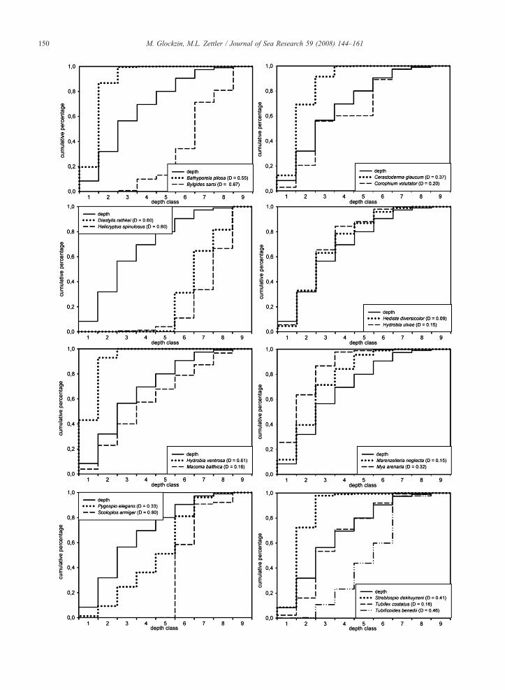
Fig. 3. Cumulative frequency distribution of depth (solid line) plottet versus s(Sachs, 1997) and given for each species, Calculated Dcritical=0,14 (p=0,05curves are not identical. Depth classification calculated after Sturges (1926), C5 (18.5 – 22), 6 (22 – 25.5), 7 (25.5 – 29), 8 (29 – 32.5), 9 (32.5- 36).

for water depth and salinity. All species examined withSpearman's rank correlation were strongly correlatedwith water depth, except the oligochaete Tubifexcostatus. The highest positive correlation factors werecalculated for a cumacean and an oligochaete: Diastylisrathkei and Tubificoides benedii. As for negativecorrelation factors, the bivalves Cerastoderma glaucumand Mya arenaria showed the highest negative depen-dency from water depth. More or less the same appliesfor salinity.D. rathkei and T. benedii again reach highestpositive correlation factors. No Spearman rank correla-tion with salinity can be proven for Corophium volutatorand T. costatus. Highest negative correlation factors withsalinity were found for C. glaucum and Bathyporeiapilosa. Remarkably, a strong negative dependencybetween median grain size and species abundancecould only be found for Macoma balthica. Three otherspecies (Bylgides sarsi, Scoloplos armiger and Hali-cryptus spinulosus) revealed less dependencies. Besidedepth and salinity, TOC ranged on third positionregarding the number of significant correlations calcu-lated. Again nearly the same correlations and species

pecies abundance. Kolmogorov-Smirnov coeffizient D calculated after, n=191) for each species curve, For (DNDcritical) the two distributionlass-nr.(depth [m]): 1 (4.5-8), 2 (8 – 11.5), 3 (11.5 – 15), 4 (15 – 18.5),


appeared as already found for water depth and salinity.T. benedii andB. sarsi show the best positive correlationswith the organic content of sediment. On the negativeside of the ordinate, species with strong and negativecorrelation factors for sediments poor in TOC do emerge.B. pilosa appeared to have the strongest negativecorrelation with TOC found for all species. Among thespecies which correlate best and positively with thesorting of sediment are B. pilosa and C. glaucum.Strongly and significantly negatively correlated with thisfactor are C. volutator, H. spinulosus, T. benedii andT. costatus. Those species which were positively in-fluenced by permeability are the amphipod B. pilosa andthe gastropod H. ventrosa. Strong but negative is thecorrelation between species abundance and permeabilityfor the oligochaete T. benedii, the amphipod C. volutatorand the polychaete B. sarsi. To a lesser degree in terms ofsignificance,H. spinulosus andM. balthica can be foundnearby on the same side of the axis.

3.3. Pearson correlation

To avoid the influence of autocorrelation, Pearsoncorrelation coefficients were calculated for the z-trans-formed data matrix containing the full set of environmentalparameters found at 78 stations (Fig. 1.). The results showmore or less strong and complex correlations betweenenvironmental variables prevailing in the Pomeranian Bay(Table 1). Water depth correlates significantly (pb0.001)positively and highest with salinity and sedimentaryorganic content (pb0.01). Permeability, on the otherhand, shows significantly (pb0.01) negative correlationswith depth. The same applies tomedian grain size (pb0.01)which is also significantly (pb0.01) negatively correlatedwith salinity. Salinity correlates significantly (pb0.001)positively with the organic content of sediments which inturn shows significantly (pb0.001) negative correlationswith all other sediment characters like median grain size,sorting and permeability. Permeability eventually correlatessignificantly (pb0.001) positively with median grain size.

3.4. Partial correlation and path analysis

In order to evaluate existing coherencies amongenvironmental parameters, and to assess the primarydescriptor predicting all other environmental variables inthe Pomeranian Bay, a partial correlation analysis (pathanalysis) was conducted according to the methodsdescribed in Legendre and Legendre (1998). Thereforeall possible and meaningful three-variable combinationswere built from a matrix of partial correlation coefficientscalculated for 6 environmental parameters sampled at 78

stations (Fig. 1) and tested (over 50 single matrices, notpresented). Depth was found as the primary descriptor forsalinity, organic content and, to a small degree, for mediangrain size. Median grain size again directly controlssorting and permeability. The organic content affects themedian grain size, sorting and permeability (interstice-blocking). Sorting again affects permeability.

3.5. Cumulative distribution curve analysis

The effect of depth as the primary descriptor on allenvironmental descriptors and, as a consequence, onspecies distribution was analysed by means of testingcumulative frequency distributions of the primarypredictor versus species abundance (Fig. 3). Congruencybetween the cumulative distribution curve of a speciesand an environmental descriptor is deemed to be ameasure of dependency among them (Jongman et al.,1987). For all species with a calculated Kolmogorov-Smirnoff coefficient D≤Dcritical (Dcritical=0.14) such adependency can be rejected with p=0.005 (Sachs, 1997).This applies to Hediste diversicolor (D=0.09) only, aspecies colonising the Pomeranian Bay apparentlyhomogenously and completely independent fromdepth. Some others, like Hydrobia ulvae (D=0.15),Macoma balthica (D=0.16), Marenzelleria neglecta(D=0.15), Tubifex costatus (D=0.16), rank as onlyslightly depth-dependent species. Often, the depth classshowing the highest difference among the cumulativedistribution curves can be regarded as an indicative valuein terms of a favoured depth range for species settlinghere. In general, the position of the species curve inrelation to the depth curve gives information about thepreferred depth range. Lies the species curve above thecurve for depth the species settles in more shallowwaters. This is obvious for Bathyporeia pilosa, Ceras-toderma glaucum, Hydrobia ventrosa and Streblospiodekhuyzeni. Others, like Bylgides sarsi, Diastylisrathkei,Halicryptus spinulosus and Tubificoides benediiprefer the deeper areas of the Bay. For Scoloplosarmiger, water depths shallower 20 m seem to be a realsettling barrier in the Pomeranian Bay.

3.6. Principal component analysis (PCA)

The usage of only one fraction of all available principalaxes for analysis will reduce interfering background noisecontained in the data. Like in our study, points (samplingstations) with same variances represent equal abundancecharacteristics. Kriging of these points allows definingareas with distinct benthic communities. The correspond-ing correlation biplot is also given (Fig. 4). The first and

Fig. 5. Display of the shift in benthic assemblage of 17 species over all zones (Fig. 4, left side). Mean abundance of single species was calculated as apercentage of total abundance per zone and normalized to 1. The feeding type, preferred substrat type and the penetration depth of each species is given.


second principal components together account for 61%of the total variance (first principal axis: 39%, secondprincipal axis: 22%). The position of the species inthe correlation biplot clearly indicates the prevailingcorrelations between them. In this respect, B. pilosa andT. benedii seem to represent some kind of “ecologicalantagonists” whereas all other species can be regarded as

Table 2Minimum/maximum values of environmental parameters and average abundzones shown in Fig. 4 (left)

Parameters Zones

1 2 3

water depth [m] 8–15 4–16 7–Salinity [psu] 7.2–7.9 5.7–8.0 6.Median grain size [μm] 178–191 110–201 80Permeability [10-6 cm s-1] 13.5–16.8 9.6–10.0 10Sorting [Folk and Ward] 0.4–0.5 0.3–0.7 0.TOC [%] 0.2–0.3 H. ulvae

(6717 ind. m-2)0.1–3.1 H. ulvae(3620 ind. m-2)

0.(2

Most abundant species per zone(average abundance)

M. arenaria(4168 ind. m-2)

M. arenaria(1171 ind. m-2)

P.(1

C. glaucum(1158 ind. m-2)

M. neglecta(645 ind. m-2)

M(3

M. neglecta(1136 ind. m-2)

B. pilosa(544 ind. M-2)

M(2

“intermediate stages” between these two extremes.Projection of the interpolated variances for the 1stprincipal components on a map of the Pomeranian Bayrevealed five areas which clearly differ in their benthicspecies composition (Fig. 4, left). Additionally, the 2ndprincipal components were also subjected to kriging andprojected separately (Fig. 4, right). Variances of species

ance of the most common species at benthic sample stations in the 5

4 5

26 11–27 15–322–13.8 7.2–11.4 7.5–12.4–335 107–348 107–270.7–31.9 11.5–49.4 4.01–11.73–1.0 0.3–1.4 0.4–0.61–1.5 H. ulvae710 ind. m-2)

0.2–9.3 P. elegans(1637 ind. m-2)

0.2–9.3 P. elegans(635 ind. m-2)

elegans251 ind. m-2)

H. ulvae(1085 ind. m-2)

M. balthica(237 ind. m-2)

. neglecta67 ind. m-2)

M. balthica(395 ind. M-2)

T. benedii (64 ind. m-2)

. arenaria98 ind. m-2)

T. benedii (389 ind. m-2) T. costatus (57 ind. m-2)

Table 3Highest Spearman rank correlation coefficients (ρnormal; ρdepth-detrended) from BIOENV procedure based on Spearman rank correlation calculatedseparately between a √√-transformed species-based similarity matrix (12 species, Bray–Curtis similarity) and two matrices of k tested environmentalfactors/-combinations sampled at 78 sampling stations

K factor /-combinations ρnormal factor /-combinations ρdepth-detrended

1 a 0.465 d 0.4472 a, c 0.552 c, d 0.4623 a, c, d 0.573 b–d 0.4894 a–d 0.576 b, d–f 0.4855 a–d, f 0.579 b–f 0.4766 a–f 0.569 - -

Factor matrix 1 (ρnormal): 6 factors, z-transformed, simple euclidean distance, Factor matrix 2 (ρdepth-fetrended): standardised residuals of 5 environmentalfactors detrended from depth by polynomial regression, simple euclidian distance. The environmental factors (a: water depth; b: near-bottom salinity;c: median grain size; d: organic content; e: sorting; f: permeability) associated to Spearman's correlation coefficients (ρnormal; ρdepth-detrended) are given.


associated with the first principal axis are responsible forthe zonation (Fig. 4, left) whereas, due to the orthogonallyrotated and maximised variances along main axes in aPCA, species variances along the second principle axisgive another picture (Fig. 4, right). First axis principalcomponents seem to divide the Bay in a North-Westdirection, second principal components apparently do italong the South-West axis. Though the calculation restssolely upon species abundance, it clearly indicatesdifferent environmental conditions such as the bottommorphology of the Pomeranian Bay (Figs. 1 and 4). Theassemblage of selected species over all 5 zones indicatedby the interpolation of the 1st principal components(Fig. 4, left) is graphically displayed and the autocology ofspecies roughly described (Fig. 5). A steady shift in

Fig. 6. Results for two separately calculated canonical correspondence analycorresponding environmental factors sampled at 78 stations. Figure A (letransformed abiotic matrix of 6 environmental factors. Species situatedc) H. diversicolor. B (right side): CCA calculated for √√-transformed abudetrended from depth. Species situated close to the center of the biplot are a

benthic species from an assemblage characterized bymolluscs and polychaetes to a more polychaete/oligo-chaete dominated community over the different zones canclearly be seen. The different environmental conditionsprevailing in each zone are described in terms ofminimum and maximum values for all abiotic parametersregarded in Table 2. Here, the most common species perarea are named and their average abundance is given.

3.7. Link between biotic and environmental patterns(BIO-ENV procedure)

The correlation factors calculated via BIO-ENV aregiven in Table 3. In the BIO-ENV analysis of the z-transformed matrix of 6 environmental parameters, the

ses (CCA) of macrobenthic species abundance data (12 Species) andft side): CCA calculated for √√-transformed abundance data and z-close to the center of the biplot are a) H. ulvae, b) M. arenaria,ndance data and matrix of standardised residuals of 5 abiotic factors) H. diversicolor, b) H. ulvae, c) M. neglecta.


single abiotic factor which is associated best with theobserved species distribution in the Pomeranian Baywas the water depth. However, its correlation factor wasoutranked by nearly all other variables calculated forfactor combinations. With a spearman's rank coefficientof about 0.465, depth alone seems to be responsible foralmost 80% of the total similarity between biotic andabiotic matrices. Adding more factors, the correlation of0.465 increases only about 0.114 up to 0.579 for a 5-factor combination of water depth, salinity, mediangrain size, organic content and sorting. For the

Table 4Results for two separately calculated canonical correspondence analysesmacrobenthic species abundance data (12 Species) and corresponding enviro

A: CCA–z-transformed abiotic matrix

Axis 1

Eigenvalue 0.129Species-environment correlations 0.826Cumulative percentage variance

Of species data 24.80Of species-environment relation 70.9

Environmental variable Inter-set correlations with

Axis 1 Axis 2 Axis

Depth 0.755 0.195 -0.01Sorting -0.385 0.285 -0.21Salinity 0.292 0.330 0.38Organic content 0.250 0.004 0.27Median grain size -0.061 -0.067 -0.14Permeability -0.217 0.111 -0.20

B: CCA - matrix of residuals detrended from depth

Axis 1

Eigenvalue 0.129Species-environment correlations 0.826Cumulative percentage variance

Of species data 24.80Of species-environment relation 70.9

Environmental variable Inter-set correlations with

Axis 1 Axis 2 Axi

Sorting -0.364 -0.188 -0.1Salinity -0.134 0.445 0.0Organic content 0.084 0.343 0.0Median grain size 0.183 -0.269 0.2Permeability 0.019 -0.328 0.2

Inter-set correlations between the first 3 canonical axes and environmental vexplained (percentage of the total variance in the species data explained) by(unique) effects describe variance explained by each environmental variableforward selection. Environmental variables are listed by the order of their inc√√-transformed abundance data and z-transformed abiotic matrix of 6 envabundance data and matrix of standardised residuals of 5 abiotic factors detr

environmental matrix undetrended from water depth,this factor combination seems to describe best thebenthic community structure which occurs in thePomeranian Bay. Noticeably, the variable water depthcan be found among almost every tested factorcombination, almost always accompanied by salinity.As for the Spearman rank correlation between the bioticand the detrended abiotic matrix, an entirely differentpicture emerges. Here, the organic content accounts forover 90% of the calculated similarity. By adding otherfactors to the matrix, only a slight increase in similarity

(CCA) including the results of Monte-Carlo permutation test ofnmental factors sampled at 78 stations

Axis 2 Axis 3

0.024 0.0180.528 0.572

29.4 32.883.9 93.6

Marginal effects Conditional effects

3

5 11% (pb0.001) 11% (pb0.001)7 4% (pb0.001) 3% (14%) (pb0.001)9 3% (pb0.001) 2% (16%) (pb0.001)5 2% (pb0.001) 1% (17%) (pb0.001)7 2% (pb0.001) 1% (18%) (pb0.001)6 1% (pb0.001) 0% (18%) (pb0.001)

Axis 2 Axis 3

0.024 0.0180.528 0.572

29.4 32.883.9 93.6

Marginal effects Conditional effects

s 3

09 3% (pb0.001) 3% (pb0.001)47 2% (pb0.001) 1% (4%) (pb0.001)93 2% (pb0.001) 2% (6%) (pb0.001)66 1% (pb0.001) 1% (7%) (pb0.001)83 1% (pb0.001) 0% (7%) (pb0.001)

ariables are presented. Marginal effects describe percentage varianceusing each environmental variable as the sole predictor. Conditionalwith the variable(s) already selected treated as covariable(s) based onlusion in the forward-selection model. Subtable A: CCA calculated forironmental factors. Subtable B: CCA calculated for √√-transformedended from depth.


can be observed. The factor combination which is linkedbest with the biotic matrix consists of salinity, mediangrain size and the organic content of the sediment.

3.8. Canonical correspondance analysis with MonteCarlo permutation

In addition to the BIO-ENV procedure, a CCA wascalculated for matrices of 78 sampling sites (Fig. 1) with√√-transformed abundance data of 12 species andcorresponding z-transformed environmental data(Fig. 6, A) and, separately, with an environmental datamatrix of standardised residuals of 5 environmentalvariables and 78 stations (Fig. 6, B). The Biplot(Fig. 6, A) and the output from the Monte-Carlopermutation test (Table 4) clearly depict the dependen-cies among environmental factors. In this environmentthe species are arranged according to their eccologicaloptima. The first and second CCA axes together accountfor ca. 84% of the relations between species and envi-ronmental conditions, highest correlated along the firstCCA axis. Water depth shows the highest correspon-dence to the first CCA axis followed by salinity andorganic content whereas all other factors are negativelycorrelated. With the second CCA axis only median grainsize shows a negative correlation, all other environ-mental factors are positively correlated. Depth andsorting together account for 16% of the overall varianceamong the environmental variables. In this setting,B. pilosa shows a high affinity to well sorted andpermeable sediments. This applies to S. dekhuyzeni andC. glaucum as well but to a lesser degree. C. volutatorand T. benedii prefer higher amounts of organic carbonin the sediment than S. dekhuyzeni and C. glaucum. B.pilosa seems to avoid these sediments completely. Withrespect to water depth, T. benedii occurs in deeper areasof the Pomeranian Bay whereas T. costatus, C. volutator,P. elegans and C. glaucum can be found in intermediatedepths. B. pilosa and S. dekhuyzeni on the other handprefer shallow waters. Species arranged towards thecenter of the plot, e.g. C. glaucum and P. elegans, eitherare unrelated to the environmental axes or find theiroptimum here. Other species such as H. ulvae,M. neglecta andH. diversicolor are situated in the centerof the plot and represented by lower case letters (a, b, c).Vice versa, species arranged more towards the border ofthe plot, e.g. B. pilosa, C. volutator and T. benedii, canbe regarded as “specialists” with reference to certainenvironmental parameters.

The biplot of the CCA calculated for speciesabundance data and environmental factors detrendedfrom depth (Fig. 6, B) shows a similar configuration of

species along the ecological vectors. But there aredifferences. First, the space of environmental vectorsseems more spread and is able to give a more detailedpicture of the abiotic background on species-environ-ment interactions. The first two axes are responsible forthe exact amount of species environment relations as itwas calculated for the first CCA biplot. Here, the firstCCA axis is positively correlated with median grain size.Sediment sorting and salinity correlate negatively withthe first axis. Permeability and organic content showonly weak correlations. All environmental factors arecorrelated stronger with the second than with the firstCCA axis. And in this ecological space, the species seemto behave in a slightly different way. M. neglecta hasmoved to the center of the biplot whereas M. arenariahas moved slightly outwards. S. dekhuyzeni formerlyassociated with low organic content and low salinity,now seems to prefer higher amounts of both factors. Thespecies P. elegans is associated with high values oforganic content and salinity in CCA biplot A, in CCAbiplot B this species prefers high permeable and goodsorted sediments of low organic content. However, bothCCA biplots show an environment strictly divided intodeep (lower permeability, bad sorting, high organiccontent, increased salinity) and shallow (good sorted,finer grained and more permeable substrate with loworganic content), areas of the Pomeranian Bay.

4. Discussion

4.1. Models

The present study was the first attempt towards abenthic – abiotic interaction model using a complex dataset of recent investigations in the Pomeranian Bay. Suchmodel allows to predict better on how and to what extentnatural or anthropogenic influences affect benthiccommunity assemblages not only in the PomeranianBay but other areas of the Baltic Sea. However, anexploratory statistical description of the prevailingecological structure of the observations made on sitealways is the indispensible first step (Bourget andFortin, 1995). The extraction of patterns of benthiccommunity distributions using large-scale studies ischaracterized by a large number of data points randomlysampled over long distances and in irregular spatialintervals. A task not easily solved by using only onestatistical method. We therefore considered the follow-ing hierarchical approach as an appropriate method ofresolution: i) detection of induced spatial dependencies,ii) examination of the environmental framework, iii)statistical description of patterns in environmental and


species data matrices, iv) combination of abiotic andbiotic matrices in order to isolate abiotic factorsresponsible for species assemblages and distributions.

4.2. Induced spatial dependences

The results of the statistical analyses using spatially andtemporally distributed data may be severely biased eitherby spatio-temporal autocorrelation (Legendre, 1993;Diniz-Filho et al., 2003) or forcing of strong gradients(Bourget et al., 1994). To avoid this, the data used in ouranalysis were testet on autocorrelation beforehand and theresults obtained were taken into account in furtheranalysis. Strong gradients can monopolise much of astatistical analysis (Bourget et al., 2003) and should beremoved before analysis unless it is the stated aim toexplore the influence of this particular gradient (Legendreand Legendre, 1998). In our case we discovered a stronggradient of depth along the North-South axis of the Bay.Correlation analysis revealed a complex framework ofabiotic interactions and simply removing one part possiblywould make it impossible to see the whole picture. Here,we have chosen a compromise and detrended the abioticmatrix but did use the untreated data set as well as initialdata applied in statistical analysis. To our knowledge, thisis the first study which takes spatial autocorrelation andtrend into account for this kind of analysis in the BalticSea.

4.3. Environmental framework

As calculated by correlation analysis, a complexframework of inter-environmental relationships shapesthe ecological background of the Pomeranian Bay. Toutilize this knowledge for further interpretation, taking acloser look on the prevailing environmental conditionsin the study area is indispensible. Due to prevailing windand wave conditions, saline water inflows from deeperareas of the Bay and fresh water from the coastal riverrunoff no homogeneous salinity zonation could develop.The deeper areas of the southern Baltic as Sassnitzrinne,Arkona and Bornholm Basin are the main accumulationareas for fine particles with input of high organicmaterial from the Pomeranian Bay (Kuhrts et al., 2006).This explains the apparent correlation between salinityand organic content, i.e. with increasing water depthsand equally rising salinity, the content of organic carbonin the sediment also increases. With increasing amountsof fine particles at the sea bottom, permeability of thesediment in turn decreases rapidly because of theblocking of the interstice (Forster et al., 2003). Due tothe glacifluviatile and glacioaeolian genesis of the Bay,

median grain size and sorting are merely modified bythe hydrography, but not created.

4.4. Pattern analysis

In order to identify environmental factors responsiblefor benthic species distribution from our complex set ofecological data, we first analysed the patterns containedin the data set of species abundance. To detectdifferences in community structure and to estimate thedegree of variations in environmental conditions,application of ordering techniques is the best alternativebecause they are more reliable than numerical classifi-cation methods, e.g. clustering techniques (Clarke andWarwick, 1998; Legendre and Gallagher, 2001). Thisproved to be true, since a valid (evaluated with anANOSIM) and sufficiently detailed zonation could notbe obtained by clustering of species abundance data (notpresented). The projection of the first principal compo-nents, calculated by a PCA of selected species abun-dance data, allows a division of the Pomeranian Bay into5 different zones with specific benthic communitycompositions with their boundaries running almostexactly along the bathymetric morphology of theBay's seafloor. Thus, the computed zonation dividesthe benthic realm of the Pomeranian Bay into shallowand deep water communities, inhabiting areas of similarsediment composition (Oder Bank and GreifswalderBodden Sill) on both sides of the Bay and areas of highand low water depths and likewise organic enrichment(Arkona Basin and Oder River mouth) in the North andSouth. The distribution of the species in the PCA biplotprovides a clear picture of interspecific correlations. Inthis reduced space, Tubificoides benedii (see Fig. 7,right picture) opposes B. pilosa (see Fig. 7, left picture),its autecological counterpart. Both species can beregarded as representatives of two extreme environ-mental conditions, with the ecological preferences of allother species examined distributed in between – apicture clearly illustrated not only by the abundanceplots but also by the results of the CCA analysis. ThePCA biplot of the 2nd principal components shows amere “orthogonal” impact of environmental factorsalong the North-South and East-West axis. From Southto North the main river runoff discharges into the Baywith a high organic input, whereas in the eastern andwestern parts remains of ancient sandunes dominate theseafloor, formed by glacial and post-glacial processes.As a consequence, species preferring such conditions,i.e. high organic content (e.g. T. benedii) or good sortedfine sand with low organic content (e.g. B. pilosa), settlehere. The distribution of the species regarded in this

Fig. 7. Abundance plots of Bathyporeia pilosa (left) and Tubificoides benedii (right) for the time period 2003 to 2006.


study according to their presence in the different zones(see Fig. 5) shows mostly filter feeders in the shallowareas of the Bay. With increasing water depth, thespecies assemblage shifts from filter feeders and grazerstoward communities dominated by deposit feeders andpredators. According to Pearson and Rosenberg (1978),Rumohr et al. (1996) and O'Brien et al. (2003) such abenthic compartmentation over depth classes may becaused by food quality or at least food availability due tohigh sedimentation and resulting accumulation rates oforganic material. Such accumulation of organic materialoccurs throughout the year in the Pomeranian Bay. Itcauses shifts in macrobenthic community assemblagesand thus is not necessarily a result of eutrophication(Pearson and Rosenberg, 1978; Zettler et al., 2006). Itseems more likely that such community shifts are typicalfor estuarine ecosystems, favoured by physical abrasion,accumulation or biological decomposition of the abovementioned organic enrichments. Together with othermajor environmental parameters, this most likely causesthe periodically occurring “bouncing” of benthic zona-tion borders (Pazdro et al., 2001; O'Brien et al., 2003).As Bonsdorff (2006) pointed out, an anthropogenicinput can cause significant changes in benthic commu-nities but a shift from an oligotrophic towards aneutrophic state may also reflect a long-term succesionalstatus of the ecosystem.

4.5. Biotic – abiotic interactions

Canonical correlations and variance analysis mirrorecological preferences of the species colonising theavailable habitat. Combined with evaluating numericalanalysis (e.g. Monte-Carlo permutation tests, ter Braak

and Smilauer, 1998) they provide a fairly accuratepicture of biotic – abiotic interactions. By performinganalysis with both the untreated and detrended data setof environmental factors we were able to detect thepredictors of benthic assemblage and to compare bothresults to gain a better estimate of the trend. Especiallyfor the BIO-ENV and CCA analyses differencesbetween results for detrended and undetrended abioticdata and between the two techniques themselves wereobvious. BIO-ENV is a technique based on thecalculation of similarity matrices, which some authors(McGarigal et al., 2000 and others) reasoned can bemisleading in case of strong gradients over longdistances (e.g. salinity), forcing a slow and steadychange in species composition. As in BIO-ENV, withthe strong gradient of water depth the results areobvious. But without the trend, the best similaritybetween biotic and abiotic environment was caused bythe organic content. With the strong correlation betweenorganic content and water depth, this factor is likely tochange drastically over relatively short distances,especially in the deeper areas of the Bay where organicmaterial accumulates (Christiansen et al., 2002). Thesame applies to salinity, with highest values in thedeeper parts of the Bay but in constantly lower amountsin shallow areas (Lass et al., 2001). Canonical corre-spondence analysis (CCA) is best applicable if thespecies response to a factor is unimodal (Legendre andLegendre, 1998). In the Monte Carlo simulation ofCCA, calculated with exactly the same data sets used inBIO-ENV, the variable sorting was responsible for mostof the variance. Not surprisingly, in path analysissalinity and organic content were the factors directlyand solely influenced by water depth. The factor sorting


seems to be merely modified by median grain size whichin turn is distributed more evenly throughout the Bay(Bobertz and Harff, 2004). This indicates that BIO-ENVseems to be better working with short and sharp gra-dients in contradistinction to CCA which most likelyprefers distinct but uniformly continuous species re-sponse. Unimodal species response has been in accor-dance with the continua concept (Pearson and Rosenberg,1978; Gray, 1984) where community structure changescontinuously along environmental gradients, each specieshaving its optimum at a different point of the gradient.Regarding this response, the CCA of detrended abioticdata depicts the autecologic behaviour of species moredetailed than the CCA with untreated ecological para-meters. Here, the length of factor axes, representing theirinfluence, is almost equal. By comparison of the CCAbiplots, the influence of depth on all other factors becomesclear. An example gives the comparison of the results fortwo species: B. pilosa and T. benedii are far apart in thespatial and autecological sense (Fig. 7). These two speciesare situated furthest apart in both CCA biplots (Fig. 6., A,B). B. pilosa, a coast-dwelling, sandlicking amphipodwhich grazes diatoms off the surface of sand grains(Nicolaisen and Kanneworff, 1969; Sundbäck andPersson, 1981) inhabits the shallow areas of the GermanPart of the Bay, the Oder Bank and the GreifswalderBodden Sill, all sea-bottom elevations of post-glacialorigin (see Fig. 7, left picture). They consist of well sortedfine sand, deposited and sorted here by postglacial aeolianprocesses. Wind and wave energy induce currents strongenough to vent these fine grained sediments and to keepthemorganic-poor through abrasion. In sharp contrast, theeuryoec and euryhaline deposit feeder T. benedii is mostabundant in sediments rich in nutrients and organic carbonwhich form a trail along the North-South axis of thePomeranian Bay, formed by the deposition of sedimentedfine material, discharged by the Oder River in greatamounts (ca. 39 kt year-1 total nitrogen, ca. 3.1 kt year-1

total phosphorus, Pastuszak et al., 2005). For thisopportunistic oligochaete, mass reproductions in areaswith high accumulation rates of organic carbon insediments are known (Diaz, 1984). Such sediments aredistributed from the Oder River mouth up to the northwestand along the submerged ancient riverbed of the Oder, theSassnitzrinne, all the way to the Arkona Basin. Thepreference of T. benedii for impermeable silty sedimentsseems to originate from his apparent tolerance ofhydrogen sulphide occurrence and oxygen deficiency(Giere et al., 1999). The environmental preferences of B.pilosa and T. benedii are very special and this is clearlyillustrated by the CCA results for the undetrended factormatrix. However, there are inconsistencies in the

autecological needs illustrated for B. pilosa by theCCA analysis of the detrended abiotic data. In thisbiplot, B. pilosa seems fairly uninfluenced by organiccontent which is regarded as an “switch-off” parametereven in small quantities for this species. Moreover, theassociation with high permeable sediments stated by theCCA – biplot of untreated abiotic parameters seems tohave vanished. Regarding the functioning of CCAanalysis, this could be caused by the simple “yes or no”response of B. pilosa to this environmental parameters.This makes the importance of specialised knowledgeclear concerning species autoecology for the inter-pretation causal coherencies when using statisticalresults (Sachs, 1997).

4.6. Factor identification

As already discussed for BIO-ENV and CCA, thebenthic colonization of the species regarded in thisanalysis is associated with depth, since the mainphysical forcings influencing species distribution aremainly driven by this primary descriptor. The depth-dependency of benthic species distribution is alsomanifested in the results concerning the estimatedcumulative curves for depth versus selected speciesabundances (Fig. 3). The indicative value for the depth-mode of certain species can be estimated simply bylooking for the highest difference between abundanceand depth curve. Notably, most species inhabitingshallow parts of the Bay have their mode in depthclass 2 (8–11.5 m). That is simply attributed to themarked elevation of the Oder Bank and the GreifswalderBodden Sill, rising in some places from about 15 mwater depth up to 7 m depth within a few meters. Thisrepresents an insurmountable barrier for many species,even more as the environmental conditions changedrastically along the slope within short distance. Ifconsidering the fact that wind and wave driven currentsperiodically sweep the surface of the Bank (Bobertz andHarff, 2004), it is clear that mainly endobenthic speciesadapted to this conditions like B. pilosa, Streblospiodekhuyzeni, Hydrobia ventrosa and Marenzellerianeglecta find their optimum here.

5. Conclusions

As already pointed out, environmental parametersdescribing sediment characteristics such as organiccontent, sorting or permeability seem to be controlledprimarily by water depth. Since this factors were found tocause highest similarity and variance between biotic andabiotic parameter, water depth could even be described as


a “masterfactor”. It is likely, through its impact on all otherfactors, to be mainly responsible for the zonation of thebenthic species studied. Such depth-dependency ofenvironmental factors and benthic zonations is not new,it has already been observed in other marine habitats aswell (e.g. Kube et al., 1996; Bonsdorff et al., 2003;Bonsdorff, 2006; O'Brien et al., 2003; Perus andBonsdorff, 2004; Kröncke et al., 2004; Warzocha, 1995;Wildish, 1977; Zettler et al., 2006). Often salinity isregarded as the one and only primary descriptor inbrackish estuarine ecosystems. Our study disputes thisassumption even thoughwe have tested this so far only forthe Pomeranian Bay. Considering that all 12 species usedin the ordination techniques are regarded as euryhalineand that the salinity doesn't vary strongly in center of thePomeranian Bay, the apparent influence of salinity as themain predictor on the benthic assemblage becomesinsignificant. By using other species and examining thespecies-environmental relationships over a greater dis-tance along a latitudinal gradient, the salinity-inducedstress on species distribution would be dominant and ourresults might differ (Bonsdorff, 2006).

Based on the application of a set of well establishedmethods our study clearly demonstrates the need to analysespecies' relationships in gradient systems such as the BalticSea where their patterns of distribution are strongly anddirectly coupled to abiotic processes. Though the repre-sented community structure may represent only a momen-tary state of the benthic colonization in the PomeranianBay, it can be used to asses biotic-environmental processes(Laine, 2003). By using different statistical methods theseabiotic/biotic interactions were modelled allowing toextend our knowledge concerning ecosystem functioning,and provide a tool to assess natural and anthropogenicforced changes in species distribution. In a next step,species response curves, calculated on the basis of thisstudy using an appropriate model (e.g. GAM or GLMmodel presented in CANOCO, ter Braak, 1988, 1989;Guisan et al., 2006) shall enable us to create a two-dimensional ecological model of the Pomeranian Bay in aGIS based approach, thus predicting species assemblagesof 12 species by two-dimensional morphological, geologi-cal or hydrological data sets.

Acknowledgements

Sincere thanks are given to Dr. Thorsten Seifert andDr. Joachim Dippner for helpful assistance regarding thebathymetrical data and mathematical calculations and toDr. Bernd Bobertz, Dr. Björn Bohling and Dr. MichaelMeyer for helpful assistance on granulometry and GIS.The paper has been improved by constructive comments

of an anonymous referee and by the proof reading andcorrections of Dr. Doris Schiedek. This project wasfunded by the German Federal Agency for NatureConservation (Federal Authority of Federal Ministry forthe Environment, Nature Conservation and NuclearSafety) with the grant number 80 285 210.

References

Austin, M.P., 1987. Models for the analysis of species' response toenvironmental gradients. Plant Ecol. 69, 35–45.

Bobertz, B., Harff, J., 2004. Sediment facies and hydrodynamic setting,a study in the south western Baltic Sea. Ocean. Dynam. 54, 39–48.

Bonsdorff, E., 2006. Zoobenthic diversity-gradients in the Baltic Sea:Continuous post-glacial succession in a stressed ecosystem. J. Exp.Mar. Biol. Ecol. 330 (1), 383–391.

Bonsdorff, E., Laine, A.O., Hänninen, J., Vuorinen, I., Norkko, A.,2003. Zoobenthos of the outer archipelago waters (N. Baltic Sea)-the importance of local conditions for spatial distribution patterns.Boreal Environ. Res. 8, 135–145.

Bourget, E., Fortin, M.-J., 1995. A commentary on current approachesin the aquatic sciences. Hydrobiologia 300/301, 1–16.

Bourget, E., Lapointe, L., Himmelman, J.H., Cardinal, A., 1994.Influence of physical gradients on the structure of a northern rockysubtidal community. Ecoscience 1, 285–299.

Bourget, E., Ardisson, P.L., Lapointe, L., Daigle, G., 2003. Environmentalfactors as predictors of epibenthic assemblage biomass in the St.Lawrence system. Estuar. Coast. Shelf Sci. 57, 641–652.

Christiansen, C., Edelvang, K., Emeis, K., Graf, G., Jähmlich, S.,Kozuch, J., Laima, M., Leipe, T., Löffler, A., Lund-Hansen, L.C.,Miltner, A., Pazdro, K., Pempkowiak, J., Shimmield, G., Shimmield,T., Smith, J., Voss, M., Witt, G., 2002. Material transport from thenearshore to the basinal environment in the Southern Baltic Sea. I,Processes and mass estimates. J. Mar. Syst. 35, 133–150.

Clarke, K.R., Warwick, R.M., 1998. Quantifying structural redun-dancy in ecological communities. Oecologia 113, 278–289.

Diaz, R.J., 1984. Short term dynamics of the dominant annelids in apolyhaline temperate estuary. Hydrobiologia 115, 153–158.

Diniz-Filho, J.A.F., Bini, L.M., Hawkins, B.A., 2003. Spatial auto-correlation and red herrings in geographical ecology. Glob. Ecol.Biogeogr. 12, 53–64.

Ellis, J., Ysebaert, T., Hume, T., Norkko, A., Bult, T., Herman, P.,Thrush, S., Oldman, J., 2006. Predicting macrofaunal speciesdistribution in estuarine gradients using logistic regression andclassification systems. Mar. Ecol. Prog. Ser. 316, 69–83.

Field, J.G., Clarke, K.R., Warwick, R.M., 1982. A practical strategyfor analysing multispecies distribution patterns. Mar. Ecol. Prog.Ser. 8, 37–52.

Folk, R.L., Ward, W.C., 1957. Brazos river bar, a study in thesignificance of grain size parameters. J. Sediment. Petrol. 27, 3–26.

Forster, S., Bobertz, B., Bohling, B., 2003. Permeability of sands in thecoastal areas of the southern Balic Sea, Mapping a grain-sizerelated sediment property. Aquat. Geochem. 9, 171–190.

Fortin, M.-J., Keitt, T.H., Maurer, B.A., Taper, M.L., Kaufman, D.M.,Blackburn, T.M., 2005. Species' geographic ranges and distribu-tional limits, pattern analysis and statistical issues. Oikos 108, 7–17.

Giere, O., Preusse, J.-H., Dubilier, N., 1999. Tubificoides benedii(Tubificidae, Oligochaeta)- a pioneer in hypoxic and sulfidicenvironments. An overview of adaptive pathways. Hydrobiologia406, 235–241.


Gray, J.S., 1984. Ökologie mariner Sedimente. Springer, Berlin.Guisan, A., Lehman, A., Ferrier, S., Austin, M., Overton, J.M.C.C.,

Aspinall, R., Hastie, T., 2006. Making better biogeographicalpredictions of species’ distributions. J. Appl. Ecol. 43, 386–392.

HELCOM, 1988. Guidelines for the Baltic Monitoring Programme forthe Third Stage; Part D. Biological Determinants. Baltic SeaEnvironmental Proceedings, vol. 27.

Jongman,R.H.G., ter Braak, C.J.F., Tongeren,O.F.R., 1987.Data analysisin community and landscape ecology. Van Pudoc, Wageningen.

Keitt, T.H., Bjørnstad, O.N., Dixon, P.M., Citron-Pousty, S., 2002.Accounting for spatial pattern when modeling organism-environment interactions. Ecography 25, 616–625.

Kolasa, J., Strayer, D., 1988. Patterns of the abundance of species, acomparison of two hierarchical models. Oikos 53, 235–241.

Kröncke, I., Stoeck, T., Wieking, G., Palojärvi, A., 2004. Relationshipbetween structural and functional aspects of microbial andmacrofaunal communities in different areas of the North Sea.Mar. Ecol. Prog. Ser. 282, 13–31.

Krumbein, W.C., Monk, G.D., 1942. Permeability as a function of thesize parameters of unconsolidated Sand. American InstituteMining and Metallurgy Engineering, Petroleum Technology,Technical Publication No. 1942.

Kube, J., Powilleit, M., Warzocha, J., 1996. The importance ofhydrodynamic processes and food availability for the structure ofmacrofauna assemblages in the Pomeranian Bay (Southern BalticSea). Arch. Hydrobiol. 138, 213–228.

Kuhrts, C., Seifert, T., Fennel, W., 2006. Modeling transport of flufflayer material in the Baltic Sea. Hydrobiologia 554, 25–30.

Lass, H.U., Mohrholz, V., Seifert, T., 2001. On the dynamics of thePomeranian Bay. Cont. Shelf. Res. 21, 1237–1261.

Laine, A.O., 2003. Distribution of soft-bottom macrofauna in the deepopen Baltic Sea in relation to environmental variability. Estuar.Coast. Shelf Sci. 57, 87–97.

Legendre, P., 1993. Spatial autocorrelation: Trouble or new paradigm?Ecology 74, 1659–1673.

Legendre, P., Gallagher, E.D., 2001. Ecologically meaningful trans-formations for ordination of species data. Oecologia 129, 271–280.

Legendre, P., Legendre, L., 1998. Numerical Ecology. Elsevier ScienceB.V., Amsterdam.

Lozán, J., Kausch, H., 2004. Angewandte Statistik für Naturwis-senschaftler. Wissenschaftliche Auswertungen, Hamburg.

McGarigal, S., Cushman, S., Stafford, S., 2000. Multivariate statisticsfor wildlife and ecology research. Springer, New York.

McManus, J., 1988. Grain size determination and interpretation. In:Tucker,M. (Ed.), Techniques in Sedimentology. Blackwell Publishers,Oxford, pp. 63–85.

Mohrholz, V., 1998. Transport-und Vermischungsprozesse in derPommerschen Bucht. Meereswiss. Ber. 33, 1–106.

Neumann, G., Bublitz, G., 1968. Seegrunduntersuchungen imwestlichen Teil der Oder-Bucht. Beitr. Meereskd. 24/25, 81–109.

Nicolaisen, W., Kanneworff, E., 1969. On the burrowing and feedinghabits of the amphipods Bathyporeia pilosa Lindstrom andBathyporeia sarsi Watkin. Ophelia 6, 231–250.

O'Brien, K., Hänninen, J., Kanerva, T., Metsärinne, L., Vuorinen, I.,2003. Macrobenthic zonation in relation to major environmentalfactors across the Archipelago Sea, northern Baltic Sea. BorealEnv. Res. 8, 159–170.

Pastuszak, M., Witek, Z., Nakel, K., Wielgat, M., Grelowski, A., 2005.Role of the Oder estuary (southern Baltic) in transformation of theriverine nutrient loads. J. Mar. Syst. 57, 30–54.

Pavlikakis, G.E., Tsihrintzis, V.A., 2000. Ecosystem Management:A Review of a new concept and methodology. Water Resour.Manag. 14, 257–283.

Pazdro, K., Staniszewski, A., Bełdowski, J., Emeis, K.-Ch., Leipe, T.,Pempkowiak, J., 2001. Variations in organic matter bound in fluffylayer suspended matter from the Pomeranian Bay (Baltic Sea).Oceanologia 43, 405–420.

Pearson, T.H., Rosenberg, R., 1978. Macrobenthic succession inrelation o organic enrichment and pollution of the marineenvironment. Oceanogr. Mar. Biol. Ann. Rev. 16, 229–311.

Perry, R.I., Smith, S.J., 1994. Identifying habitat associations ofmarine fishes using survey data: An application to the NorthwestAtlantic. Can. J. Fish. Aquat. Sci. 51, 589–602.

Perus, J., Bonsdorff, E., 2004. Long-term changes in macrozoobenthosin the Aaland Archipelago, northern Baltic Sea. J. Sea Res. 52 (1),45–56.

Rumohr, H., Bonsdorff, E., Pearson, T.H., 1996. Zoobenthic successionin Baltic sedimentary habitats. Archive of fishery and marineresearch/Archiv für Fischerei-und Meeresforschung. Stuttgart,Jena. 44 (3), 179–213.

Sachs, L., 1997. Angewandte Statistik. Anwendung statistischerMethoden. Springer, Berlin.

Simpson, M.R., Walsh, S.J., 2004. Changes in the spatial structure ofGrand Bank yellowtail flounder, testingMacCall's basin hypothesis.J. Sea Res. 51 (3-4), 199–210.

Sturges, H.A., 1926. The choice of a class interval. J. Amer. Sci. Assoc.65–66.

Sundbäck, K., Persson, L.-E., 1981. The effect of microbenthicgrazing by an amphipod, Bathyporeia pilosa, Lindström. KielerMeeresforsch. 5, 573–575.

ter Braak, C.J.F., 1988. CANOCO- an extension of DECORANA toanalyze species-environment relationships. Plant Ecol. V 75 (3),159–160.

ter Braak, C.J.F., 1989. CANOCO- an extension of DECORANA toanalyze species-environment relationships. Hydrobiologia 184 (3),169–170.

ter Braak, C.J.F., Smilauer, P., 1998. CANOCO Reference Manual anduser's guide to Canoco for Windows, software for CanonicalCommunity Ordination (Version 4). Microcomputer Power, Ithaca,NY.

Warzocha, J., 1995. Classification and structure of macrofaunal commu-nities in the southern Baltic. Arch. Fish. Mar. Res. 42, 225–237.

Wildish, D.J., 1977. Factors controlling marine and estuarinesublittoral macrofauna. Helgol. Meeresunters. 30, 445–454.

Young, L.J., Young, J.H., 1998. Statistical Ecology, A populationperspective. Kluwer Academic Publisher, Dordrecht.

Zettler, M.L., Gosselck, F., 2006. Benthic assessment of marine areasof particular ecological importance within the German Baltic SeaEEZ. In: Nordheim, H., von Boedeker, D., Krause, J.C. (Eds.),Progress in Marine Conservation in Europe – NATURA 2000 sites inGerman offshore waters. Springer-Verlag, Berlin, pp. 141–156.

Zettler, M.L., Röhner, M., Frankowski, J., 2006. Long term changes ofmacrozoobenthos in the Arkona Basin (Baltic Sea). Boreal Env.Res. 11, 247–260.

Zettler, M.L., Schiedek, D., Bobertz, B., 2007. Benthic biodiversityindices versus salinity gradient in the southern Baltic Sea. Mar.Pollut. Bull. 55, 258–270.

spatial macrozoobenthic distribution patterns in relation ...€¦ · spatial macrozoobenthic...

Documents