flow-induced effects of macrozoobenthic structures on the ... · iii studium: 25.8.1988...
TRANSCRIPT

Flow-induced effects ofmacrozoob enthic s tructures onthe near-bed sediment t ransport
Dissertation zur
Erlangung des akademischen Grades
doctor rerum naturalium (Dr. rer. nat.)
der Mathematisch-Naturwissenschaftli chen Fakultät
der Universität Rostock
vorgelegt von
Hans Michael Friedrichs, geb. am 29. Mai 1969 in Hamburg
aus Rostock
Rostock, 15. Januar 2004

Gutachter der Arbeit:
Prof. G. Graf, Universität Rostock
Prof. M. Hüttel, Florida State University, USA
Prof. E. Pasche, TU Hamburg-Harburg
Datum der Verteidigung: 16.12.2003

most biologists
who have heard
of the boundary
layer have the fuzzy
notion that it's a distinct
region rather than the distinct
notion that it's a fuzzy region. (S. Vogel)
"Life in moving fluids", 1994

i
Erklärung
Nach § 4 Abs. 1 der Promotionsordnung der Mathematisch-Naturwissenschaftli chenFakultät der Universität Rostock vom 5. Juni 2000:
Hiermit versichere ich, die vorliegende Arbeit selbständig angefertigt und ohne fremdeHil fe verfasst zu haben. Ich habe keine anderen als die von mir angegebenen Hil fsmittel undQuellen dazu verwendet und den benutzten Werken inhaltli ch oder wörtli ch entnommeneStellen als solche kenntlich gemacht.
Declaration
I certify that this thesis was entirely written by me and without any external assistance. Itcomprises only my own original work, and due acknowledgement has been made in the textto all other material used.
Rostock, ....................................................................................

ii
Lebenslauf
Diplom-Biologe Michael Friedrichs
Zur Person:
Vor- und Nachnamen Hans Michael Friedrichs
Geburtsdatum 29. Mai 1969
Geburtsort Hamburg
Wohnort Borwinstr. 28, 18057 Rostock, Tel. 0381 – 203 29 25
Eltern Vater Dieter Friedrichs, Dipl. Volkswirt, Dr. rer. pol.
Mutter Gisela Friedrichs (geb. Woldert), Realschullehrerin
Staatsangehörigkeit Deutsch
Familienstand ledig
Schulausbildung :
1975 - 1978 3 Jahre Grundschule an der Französischen Schule „ÉcoleConsulaire St Exupéry“ in Ouagadougou (Burkina Faso)
1978 - 1980 2 Jahre Grundschule in der deutschsprachigen Abteilung der„Europäischen Schule II“ in Brüssel (Belgien)
1980 - Dezember 1982 2½ Jahre Gymnasium in der deutschsprachigen Abteilung der„Europäischen Schule II“ in Brüssel (Belgien)
Januar 1983 - 1986 3½ Jahre Gymnasium am Französischen „Lycée Labourdonnais“ inCurepipe (Mauritius).
1986 - 1988 2 Jahre Gymnasium in der deutschsprachigen Abteilung der„Europäischen Schule II“ in Brüssel (Belgien)
Schulabschluß:
Juli 1988 Europäisches Abitur (allgemeine Hochschulreife) der„Europäischen Schule II“ in Brüssel (Belgien) mit derDurchschnittsnote 82% bestanden (in Düsseldorf gemäߧ14 GV. NW. 1980 auf die Note 1.3 festgelegt)

iii
Studium:
25.8.1988 Immatrikulation zum Biologiestudium an der„Christian-Albrechts-Universität zu Kiel“
November 1990 Vordiplomprüfungen im Studiengang Biologie (Diplom) an der„Christian-Albrechts-Universität zu Kiel“ .
31.3.1997 Exmatrikulation von der „Christian-Albrechts-Universität zu Kiel“nach Abschluß der Diplomprüfungen
Studienabschluß:
August 1996 Biologie-Diplom an der „Christian-Albrechts-Universität zu Kiel“mit Hauptfach Biologische Meereskunde und den NebenfächernZoologie und Physikalische Ozeanographie;Durchschnittsnote sehr gut
Wissenschaft li cher Werdegang:
04/1997 - 09/1997 6-Monatiger Arbeitsvertrag am NIOO-CEMO in Yerseke, NL(Nederlands Instituut voor Oecologisch Onderzoek – Centrum voorEstuariene en Mariene Oecologie)für eine Pilot-Studie am Strömungskanal
10/1997 - 07/1999 Wissenschaftli cher Angestellter an der Universität Rostock,im Fachbereich Biologie, Abteilung Meerebiologie,(EU-Projekt BASYS, Baltic Sea System Study)
04/1998 1-Monatige Kooperation mit dem NIOO-CEMO in Yerseke, NL(EU-Projekt PHASE, Physical Forcing and Biogeochemical Fluxesin Shallow Coastal Ecosystems)
08/1999 - 10/1999 Arbeitslos gemeldet in Rostock
11/1999 Eintrag zum Promotionsstudium an der Universität Rostock(Abteilung Meeresbiologie bei Prof. G. Graf)
03/2000 - 03/2003 Wissenschaftli cher Angestellter an der Universität Rostock(BMBF-Projekt DYNAS, Dynamik Natürlicher und AnthropogenerSedimentation)
04/2003 - 09/2003 Wissenschaftli cher Angestellter an der Universität Rostock(EU-Projekt BIOFLOW, Flume Facili ty Co-operation Network forBiological Benthic Boundary Layer Research)
Seit 10/2003 Exmatrikuliert und arbeitssuchend gemeldet

iv
Zusammenfassung
Die vorgelegte Arbeit war Teil eines vom Deutschen Bundesministerium für Bildung undForschung (BMBF) geförderten Projektes über die Dynamik natürlicher und anthropogenerSedimentation in der Mecklenburger Bucht der Ostsee (DYNAS). Das Hauptziel der Arbeitwar die Quantifizierung der passiven Wechselwirkungen zwischen biogen erzeugten Struktu-ren, der bodennahen Strömung und dem Transport partikulären Materials.
Aktuelle Weiterentwicklungen der Methoden verhelfen zu einem besseren Einblick indiese Prozesse und ermöglichen die Lösung von bislang unbeantworteten Fragen. Ein miteinem Akustik-Doppler Strömungssensor sowie einem Bodenrelief-Laser ausgestatteter La-bor-Strömungskanal wurde für detailli erte, eingriffsfreie Messungen der Umströmung und desSedimenttransportes um biogene Strukturen eingesetzt. Diese Strukturen waren Nachbautentypischer Makrozoobenthosarten der Mecklenburger Bucht: Wurmröhre, Schneckenhaus,Muschel, Sandhügel, Trichter und quer verlaufende Kriechspur.
Die Strömungs- und Sedimentverteilungseffekte wurden zunächst an Einzelstrukturenuntersucht. Der Strömungsabriss im Umfeld der aus dem Sediment herausragenden Struktu-ren trennt einen äußeren Umströmungsbereich von einem inneren Bereich mit charakteristi-schen Verwirbelungen. Bei Strömungsgeschwindigkeiten unterhalb der Erosionsschwelle desverwendeten Sandes (220 µm) trat die Deposition von Schwebstoffen überwiegend im äuße-ren Bereich auf, wogegen Erosion und partielle Redeposition auf den inneren Bereich be-schränkt waren. Zeitserien der Erosionsabläufe zeigten einen raschen Anstieg der transpor-tierten Sedimentmenge, gefolgt von einer Abnahme bis zum Erreichen eines Gleichgewichts-zustandes. Die Sedimentvertiefungen (Trichter und Kriechspur) erzeugten nur schwacheStrömungsänderungen und einen geringen Sedimenttransport, abgesehen von der hohen De-position in der Kriechspur. Der mittlere Erosionsexport aller Einzelstrukturen betrug268 cm3 m-2, die lokale Umlagerung 319 cm3 m-2 und die mittlere Deposition betrug1154 cm3 m-2.
Anschließend wurde die Besiedlungsdichte eines Röhrenrasens sowie einer Muschelbankschrittweise erhöht. Der prozentuale Anteil der Gesamtfläche, den diese Strukturen bedeckten,wurde mit "Bedeckungsgrad" (roughness density, RD) bezeichnet. Bei niedrigen Bedek-kungsgraden erzeugte jede Wurmröhre eigene Strömungseffekte und hatte eine destabili sie-rende Wirkung auf das umgebende Sediment. Der Erosionsschwellwert lag bei RD-Wertenvon 0.6% und 1.0% zwischen 61% und 76% des Kontrollwertes von unbesiedeltem Sand.Mittlere Bedeckungsgrade von 2-4% bewirkten eine zunehmende Strömungsberuhigung zwi-schen den Strukturen, sowie eine vertikale Überströmung des gesamten Feldes. Der Erosions-schwellwert stieg dabei von 93% des Kontrollwertes bei 1.7% RD auf 104% bei 3.9% RD.Dementsprechend nahm die Erosion im Röhrenrasen ab, ebenso wie auch die Deposition.

v
Letztere lag deutlich unterhalb von der im unbesiedelten Kontrollversuch deponierten Menge.Dieser Zustand trat in der Muschelbank jedoch erst bei 8% Bedeckungsgrad auf und unter-strich damit die Bedeutung der Objektform für die erzeugten Effekte (die Röhren warenschlank und ragten weit ins Wasser hinaus, wogegen die Muscheln flach und breit auf demBoden lagen).
In einem dritten Versuchsaufbau wurden die Effekte einer künstlichen Benthosgemein-schaft untersucht, deren Artenzusammensetzung und Verteilung dem durchschnittli chen Vor-kommen auf sandigem Untergrund in der Mecklenburger Bucht entspricht. Die Strömungsef-fekte und der Sedimenttransport dieser Gemeinschaft waren trotz des hohen Bedeckungsgra-des von 9.6% geringer als bei vergleichbaren Ansätzen mit nur einer einzelnen Art. Die mitt-lere Strömungsberuhigung innerhalb der Gemeinschaft betrug lediglich 53%. Der Erosions-export (352 cm3 m-2) und die lokale Umverteilung (157 cm3 m-2) waren auf die Nähe dergroßen Strukturen begrenzt, wogegen die Deposition deutlich über dem Kontrollwert lag undsogar die Ergebnisse der anderen Besiedlungsdichte-Versuche übertraf (962 cm3 m-2). Dadiese Artengemeinschaft große Teile der Mecklenburger Bucht bedeckt, müssen ihre Sedi-mentstabili sierung und der erhöhte Partikelfang eine bedeutende Rolle für den Sedimenttrans-port im Untersuchungsgebiet spielen.
Summary
The present study was part of a national German project on the dynamics of natural andanthropogenic sedimentation (DYNAS) in the Mecklenburg Bight, Baltic Sea, funded by theFederal Ministry for Education and Research (BMBF). Its objective was to quantify thepassive interactions between biogenic structures, the near-bed flow regime and the transportof particulate matter.
Recent method improvements enable deeper insights into these processes and provideways to solve questions that remained unanswered in the past. A laboratory flume channel,equipped with an acoustic Doppler flow sensor and a bottom scanning laser system, was usedfor detailed, non-intrusive measurements of the flow field and of the sediment transportaround biogenic structures. The structures were replicates of typical macrozoobenthic speciescommonly found in the Mecklenburg Bight: a worm tube, a snail shell , a mussel, a sandmound and pit, and a cross-stream track furrow.
The flow and sediment transport effects were first studied on solitary structures. Flowseparation around the protruding structures divided an outer deflection region from an innerregion with characteristic vortices. At flow velocities below the erosion threshold of the sur-rounding bare sand (220 µm), deposition of suspended matter mainly occurred in the outerregion, whereas sediment erosion and a partial redeposition were found in the inner region.Erosion time-series displayed a rapid transport peak, followed by decaying intensities until an

vi
equili brium state was reached. The cavities (track and pit) only produced weak flow effectsand low sediment transport magnitudes, except a high deposition inside the track. The averageerosion export of the solitary structures was 268 cm3 m-2, the local displacement around thestructures was 319 cm3 m-2, and the average deposition was 1154 cm3 m-2.
The population densities of a worm tube lawn and of a mussel bed were then graduallyincreased. The percentage of the bed surface covered by these roughness elements was termed"roughness density" (RD). At low RD values, each worm tube structure independently gene-rated flow effects and had a destabili sing influence on the sediment. The erosion thresholdwas between 61% and 76% of the bare sand control value at RD 0.6% and 1.0% respectively.At intermediate roughness densities around 2-4% RD, the flow speed was gradually reducedinside the arrays and deflected over the structures. The erosion resistance increased to valuesbeyond those of bare sand, switching from destabili sing to stabili sing effects (93% of thecontrol threshold at RD 1.7% and 104% at RD 3.9%). The erosion consequently was reduced,as well as the deposition, which remained well below the level of the bare control surface.This status was delayed to a RD of 8% in the mussel bed, showing a shape-dependent differ-ence between the effects of slender tubes and flat mussels.
A third set of experiments was focussed on the effects of an artificial benthic community,reflecting the species composition and distribution commonly found on sandy sediments inthe Mecklenburg Bight. Although this layout had a roughness density of 9.6%, its flow andsediment transport effects were weaker than in comparable single-species assemblages. Theoverall flow reduction within the community was 53%. The erosion export (352 cm3 m-2) anddisplacement (157 cm3 m-2) were restricted to local effects of large structures. In contrast, thedeposition volume ranged well above the control and exceeded the results of all roughnessdensity experiments (962 cm3 m-2). As the community covers large parts of the MecklenburgBight, it is concluded that the combined sediment stabili sation and enhanced particle captureplay an important role for the sediment transport in the study area.

vii
Contents
1 Introduction 1
2 Materials and methods 4
2.1 Project background.....................................................................................................42.2 Project-related study site............................................................................................42.3 Instrumentation...........................................................................................................6
2.3.1 Flume channel ................................................................................................72.3.2 Flow measurements........................................................................................82.3.3 Laser bottom scanner......................................................................................92.3.4 Positioning software.....................................................................................10
2.4 Near-bottom flow theory..........................................................................................112.4.1 General aspects.............................................................................................112.4.2 The benthic boundary layer region...............................................................12
2.5 Experimental design.................................................................................................152.5.1 Biogenic structures.......................................................................................152.5.2 Experimental conditions...............................................................................17
2.6 Data treatment ..........................................................................................................21
3 Results 25
3.1 Control measurements..............................................................................................253.2 Solitary biogenic structure effects............................................................................27
3.2.1 Flow regime around the structures...............................................................273.2.2 Solitary structure erosion experiments.........................................................353.2.3 Solitary structure deposition experiments....................................................40
3.3 Roughness density effects........................................................................................423.3.1 Flow interactions..........................................................................................423.3.2 Roughness density-related sediment transport .............................................43
3.4 Artificial macrobenthic community .........................................................................473.4.1 Flow regime modifications of the community .............................................473.4.2 Sediment transport in the artificial community ............................................49
4 Discussion 53
4.1 Solitary structures.....................................................................................................534.1.1 Near-bed flow around solitary structures.....................................................534.1.2 Sediment transport processes around the solitary structures........................56
4.2 Effects of increasing roughness densities.................................................................614.2.1 Alterations of the near-bed flow in the presence of roughness elements.....61

viii
4.2.2 Sediment transport through the roughness element arrays...........................634.3 Passive effects of an artificial macrobenthic community.........................................664.4 Conclusions..............................................................................................................70
5 Reference list 71
5.1 Personal communications.........................................................................................715.2 Manuscripts..............................................................................................................715.3 References................................................................................................................71
Acknowledgements 80
List of tables
Table 2.1: Dimensions of the artificial biogenic structures deployed in the experiments......17
Table 2.2: Reynolds numbers of different characteristic length scales of the flume..............20
Table 3.1: Flow velocities and stress levels behind the solitary structures.............................33
Table 3.2: Solitary structure erosion and deposition results...................................................41
Table 3.3: Summary of the roughness density-dependent sediment transport results............47
Table 4.1 Flow conditions and sediment stabili ty properties for the roughness densities.....65
List of figures
Fig. 2.1: Map of the western Baltic Sea and DYNAS area....................................................5
Fig. 2.2: BSH model predictions of the surface currents near Kühlungsborn........................6
Fig. 2.3: Illustration of the flume channel design...................................................................7
Fig. 2.4: Layout and principle of operation of the acoustic Doppler velocimeter (ADV) .....8
Fig. 2.5: Layout and principle of operation of the laser bottom scanner..............................10
Fig. 2.6: Schematic diagram of the vertical structure of the benthic boundary layer...........14
Fig. 2.7: Theoretical boundary layer formation in the flume. ..............................................15
Fig. 2.8: Synopsis of the solitary structures used.................................................................16

ix
Fig. 2.9: The tube lawn and mussel roughness density layout .............................................16
Fig. 2.10: The species responsible for biogenic structures in the study area.........................17
Fig. 2.11: Layout of the current velocity measurements........................................................18
Fig. 2.12: Summary of the experimental conditions..............................................................20
Fig. 2.13: Example of a vertical velocity profile analysis......................................................22
Fig. 2.14: Calculation of sediment transport and local displacement.....................................24
Fig. 3.1: Longitudinal flow velocity section through the control layout..............................25
Fig. 3.2: Roughness length z0 extracted from the x,z planar section at 2 cm s-1 ..................26
Fig. 3.3: Thickness of the deposed marl layer in the control experiment ............................26
Fig. 3.4: Details of the effects of worm tube, snail shell and track on the main flow..........27
Fig. 3.5: Main flow component U, longitudinal sections through the solitary structures....28
Fig. 3.6: Roughness length distribution around the solitary structures................................29
Fig. 3.7: Vertical flow W in longitudinal sections through the solitary structures ..............30
Fig. 3.8: Cross-stream (V) and vertical (W) flow in planar (x,y) horizons at 2 cm s-1 ........31
Fig. 3.9: Vertical velocity and Reynolds stress profiles around the solitary structures.......32
Fig. 3.10: Reynolds stress 1 cm downstream of the structures and flow recovery withincreasing downstream distance from a mussel (Mytilus edulis) assemblage. ......33
Fig. 3.11: Flow visualisation experiments with potassium permanganate (KMnO4) dye......34
Fig. 3.12: Bottom relief after the solitary structure erosion experiments...............................36
Fig. 3.13: Erosion along the centreline of each solitary structure..........................................36
Fig. 3.14: Differential erosion graphs of the solitary structure erosion..................................37
Fig. 3.15: Flow regime around the sand mound, measured before and after the erosion.......38
Fig. 3.16: Erosion sequence of the worm tube layout ............................................................39
Fig. 3.17: Erosion export and local displacement sequences of the solitary structures.........39
Fig. 3.18: Differential graphs of the solitary structure deposition.........................................41
Fig. 3.19: Flow velocity effects of increasing worm tube roughness densities......................42
Fig. 3.20: Influence of the roughness densities on the relative vertical flow velocity...........43
Fig. 3.21: Differential roughness density erosion plots and transport magnitudes................44
Fig. 3.22: Critical erosion thresholds of the solitary structures and roughness densities.......45
Fig. 3.23: Deposition at increasing roughness densities RD (worm tubes and mussel).........46

x
Fig. 3.24: Effects of an artificial community along three parallel longitudinal sections.......48
Fig. 3.25: Flow effects of an artificial community on the roughness length z0......................49
Fig. 3.26: Flow effects of an artificial community in planar horizons...................................50
Fig. 3.27: Sediment erosion inside an artificial community...................................................51
Fig. 3.28: Sediment deposition inside an artificial community..............................................52
Fig. 3.29: Cross-stream averages of the deposition intensity in the artificial community .....52
Fig. 4.1: Flow distribution around an obstacle, modified after Shamloo et al. (2001).........54
Fig. 4.2: Flow distribution across a pit-li ke depression........................................................55
Fig. 4.3: Superposed erosion pattern and vertical flow around a worm tube.......................57
Fig. 4.4: Cross-stream diverging flow around the sand mound...........................................58
Fig. 4.5: Sediment transport processes around the solitary mussel structure.......................59
Fig. 4.6: Decay of the local sediment transport rates around the solitary structures............60
Fig. 4.7: Illustration of independent, interactive and skimming flow conditions.................62
Fig. 4.8: Side-view picture of the artificial community .......................................................66
Fig. 4.9: Overview of the sediment transport values at increasing roughness densities......68
Symbols and abbreviations
List of symbols
Cr correction factor in the roughness length formula (Dade et al., 2001)
δ, δDBL, δVSL boundary layer thickness, DBL thickness and VSL thickness [cm]
e base of the natural logarithm; the symbol "e" honours L. Euler: ~ 2.71828...
κ von Karman constant (~ 0.41)
ks sediment grain size [cm]
kr roughness element height [cm]
ν kinematic viscosity of the fluid (30 ppt. seawater, 20°C: 1.047 10-6 m2 s-1)
π "Pi", the ratio of a circle's circumference to its diameter: ~ 3.14159...
ρ density of the fluid (30 ppt. seawater, 20°C: 1.024 103 kg m-3)
-ρ[U'W'] Reynolds stress, or turbulent shear stress [N m-2]

xi
Re, Re*, Rex Reynolds number, roughness Reynolds number, local Reynolds number
RD roughness density: percentage of the bed area covered by the objects [%]
τ0 bed shear stress [N m-2]
U horizontal, longitudinal flow velocity component [cm s-1]
U' flow fluctuation around the mean horizontal flow U [cm s-1]
U∞ , Umax free-stream flow velocity [cm s-1]
U* bottom shear (friction) velocity [cm s-1]
Ucrit , U* crit erosion threshold values, either expressed as free-stream or shear velocity
[U] average value of the horizontal flow velocity component U [cm s-1]
[U'W'] product of the fluctuation of U and W; part of the Reynolds stress [cm2 s-2]
U(z) horizontal flow velocity at a height z above the boundary [cm s-1]
UW vector length term, e.g. in the vector addition: 22 WU UW +=
V cross-stream (lateral) flow velocity component [cm s-1]
W vertical flow velocity component [cm s-1]
x streamwise co-ordinate in the flume channel positioning system [m]
y cross-stream co-ordinate in the flume channel positioning system [m]
z vertical co-ordinate in the flume channel positioning system [m]
z0 bottom roughness length parameter [cm]
Abbreviations
3D 3-dimensional
ADCP Acoustic Doppler Current Profiler
ADV A coustic Doppler Velocimeter
BBL Benthic Boundary Layer
BMBF German Federal Ministry for Education and Research
BML Benthic Mixed Layer
BNL Benthic Nepheloid Layer
BSH German Federal Maritime and Hydrographic Agency
ca. circa, approximately
cf. confer, refer to
CMOS Complementary Metal-Oxide Semiconductor
DBL Diffusive Boundary Layer
DYNAS Dynamics of Natural and Anthropogenic Sedimentation (BMBF project)
e.g. exempli gratia, for instance
Excel Microsoft Excel, spreadsheet software
xii
GIS Geographical Information System
Hi8 Camcorder video recording standard
i.e. id est, that is to say
IOW Baltic Sea Research Institute, Rostock Warnemünde
KMnO4 potassium permanganate
LUNG Regional State Off ice for the Environment, Nature Conservation andGeology (Mecklenburg-Western Pommerania, Germany)
NorTek NorTek AS, Vangkroken 2, 1351 Rud, Norway
PC Personal Computer
pixel picture element
POC Particulate Organic Matter
ppt parts per thousand
PVC Polyvinyl Chloride [-CH2-CHCl-]n
RS-422 serial port interface communication standard
Surfer Surface mapping system, Golden Software Inc., 809 14th street, Golden,Colorado 80401-1866, USA
TechnoTrans TechnoTrans, Carl-Hopp-Straße 19a, 18069 Rostock, Germany
TPM Total Particulate Matter
VSL Viscous Sublayer
WISTMAK project on relevant macrozoobenthic species for the creation of biogenicstructures in the coastal waters of Mecklenburg-Western Pommerania,supported by the Ministry of the Environment of Mecklenburg-WesternPommerania and LUNG

Introdu ction
1
1 Introdu ction
"The sea floor rarely is smooth" is how Yager et al. (1993) began their article on passivedeposition to pits. This rather general statement is particularly true for coastal and shallowwaters. Despite a high spatial heterogeneity, sediment surfaces in these regions usually arecharacterised by large quantities of biogenic structures (Wheatcroft, 1994). These structurescan either consist of the organism body by itself, or they can be a variety of different tracessuch as mounds, pits or tracks. Many benthic organisms depend directly or indirectly on theinteraction with the surrounding flow for their nutrient supply, reproduction and waste disper-sal. Some of these exchange processes are controlled by the active behaviour of the organ-isms, but the presence of their biogenic structures in the near-bed flow also induces passiveinteraction effects (Graf and Rosenberg, 1997). The effects of these biogenic structurestherefore have to be included in a study of the near-bed flow dynamics and of the particulatematter transport or carbon fluxes.
Deposit feeders were found to ingest more microphytobenthic algae, whereas suspensionfeeders mainly graze on pelagic algae (Muschenheim, 1987; Herman et al., 2000). Increasedflow speeds or elevated particulate fluxes were seen as a cue for facultative suspension feed-ers to switch their feeding mode (Taghon et al., 1980; Dauer et al., 1981; Bock and Mill er,1997). Abelson et al. (1993) proposed that slender bodies in the near-bed flow were betteradapted to catch small suspended particles, whereas flat bodies were expected to feed on highfluxes of bedload particles. Isolated tube-building worms can thus considerably take advan-tage of the passive flow interaction caused by their tube, which increases the residence time ofparticles near the feeding appendages (Carey, 1983) and assists the resuspension of organic-rich fluff and aggregates (Eckman and Nowell , 1984). The flow interaction of protruding bio-genic structures generates enhanced fluxes towards local microhabitats of associated faunaaround the structures (Eckman, 1985). In addition, these fluxes can considerably increase thepore-water exchange and the transport of dissolved or particulate matter into - and out of - thesediment (Hüttel and Gust, 1992; Hüttel and Rusch, 2000). Pressure gradients related to theexposure to specific flow speeds at different heights within the boundary layer provide themotor of purely passive pumping mechanisms. This principle is used for e.g. the irrigation ofArenicola marina burrows (Vogel, 1994) or egg-tending fish burrows (Takegaki andNakazono, 2000). The suspension-feeding of sponges or ascidians also is known to rely onpassive pumping assistance (Vogel, 1994). Suspension feeding bivalves risk high refilt rationrates (O'Riordan et al., 1995). Dense populations of e.g. the mussel Mytilus edulis thereforedepend on turbulent mixing for both, food supply and the dumping of biodeposits (Fréchetteet al., 1989; Butman et al., 1994; Widdows et al., 2002). The spatial distribution within mus-sel beds was shown to be spatially ordered in complex patterns predictable by fractal geome-

Introdu ction
2
try, for which the importance of f low interaction for the transport of nutrients and for larvalattachment was discussed as a possible reason (Snover and Commito, 1998). Larval settle-ment in general strongly depends on the flow conditions in the recruitment area, and the pres-ence of adult conspecifics can either have positive or negative consequences (Grégoire et al.,1996; Abelson and Denny, 1997; Crimaldi et al., 2002). Bioturbating organisms have beenreported to influence the resuspension of sediments by their active behaviour at low flowspeeds (Davis, 1993; de Deckere et al., 2000), but also through passive effects li ke reducederosion thresholds caused by infaunal reworking or surface modifications. The latter are thegrazing of biofilms as well as motion tracks (Nowell et al., 1981; Widdows et al., 2000;Andersen et al., 2002). These tracks can in return increase the deposition of f luffy material.Enhanced deposition to pits (Yager et al., 1993) also has a positive influence on the foodcapture of deposit-feeding organisms like the bivalve Macoma balthica (Brafield and Newell ,1961), the lugworm Arenicola marina, or spionid polychaetes (Eckman et al., 1981). The spi-onid tube-building worm Polydora cili ata was reported to cause high deposition rates of up to50 cm within 21 days (Daro and Polk, 1973) and to stabili se the sediment in the presence ofthe worm tubes (Noji and Noji , 1991). Widdows and Brinsley (2002) identified key speciesand crucial processes for the stabili ty of the sediment surface and discuss their influence onthe sediment transport in the intertidal zone.
The study of macrobenthic interaction with the surrounding flow regime and the sedimentstabili ty discussion thus are topics that have already been treated before. However, some ofthe conclusions were mainly based on assumptions instead of direct measurements (Rhoads etal., 1978; Luckenbach, 1986), and many questions thus remained unanswered, as pointed outin a review by Graf and Rosenberg (1997). Nowell and Jumars (1984) state in theirconclusions, that "despite the weight of the evidence, mechanisms responsible for eco-logically important flow effects remain poorly identified, poorly parameterized, and largelyunquantified". Most of the previous studies focus on the effects of a single species, and thecomplex interaction within communities were not yet documented. Some authors (e.g. Asmusand Asmus, 1998; Thomsen and Jähmlich, 1998) measured in-situ carbon fluxes across com-munities, but the topography and the exchange mechanisms were not included into thesestudies. Jumars and Nowell (1984) conclude in their review on the effects of benthos onsediment transport, that a consistent functional grouping of organisms as stabili sers or desta-bili sers is not possible, especially because of manifold behaviour nuances.
Recent improvements of the relevant methods have produced new tools for a better anddeeper insight into these processes (Lohrmann et al., 1995; Butman et al., 1994; Stamhuis andVideler, 1995; Wheatcroft, 1994; Butler et al., 2002; Røy et al., 2002). In fact, the develop-ment of high-resolution techniques for non-intrusive measurements of either the flow regime(Doppler velocimetry, particle image velocimetry) or the bottom mapping (photogrammetry,laser profilometry) is still i n progress. The combination of both, flow measurement and bot-tom scanning techniques, was mainly used in hydraulic engineering in the past and is rela-

Introdu ction
3
tively new to benthic biology. Hydraulic research, and particularly topics related to piers andbridge abutment erosion, resulted in a variety of detailed studies on the interactions betweensubmersed objects, the flow regime and the sediment. Some of the recent publications are, e.g.Kothyari and Ranga Raju (2001), Sumer et al. (2001), Graf and Istiarto (2002). These studieswere mainly focussed on singular shapes and simple arrangements. In contrast, the diversityof the biogenic structures found in benthic communities, and their manifold flow interactioneffects occurring simultaneously on several scales, were not yet addressed by many authors(Fries et al., 1999; Madsen et al., 2001; Andersen et al., 2002; Widdows and Brinsley, 2002).The central hypothesis of the present study therefore was to combine modern techniques inorder to test if the passive flow interactions of biogenic structures have a significant effect onthe transport of sediments and suspended matter. Due to the need for a comprehensive set oftests performed under identical conditions, it also retraces some published experiments.
Resuming preliminary works of the author on the flow reduction in artificial polychaetetube lawns (Friedrichs, 1996; Friedrichs et al., 2000), the intention of the present study was toelucidate the passive modifications of the near-bed flow regime caused by biogenic structures,and to quantify their influence on the transport of particulate matter. Laboratory flume chan-nel experiments were designed to provide a deep insight into these processes under steadyflow conditions. The specific beach fauna was however excluded, as well as wave and tidalcurrents. A selection of typical biogenic structures generated by macrozoobenthic speciescommonly found on sandy sediments of the study area, i.e. the Mecklenburg Bight, was there-fore reproduced in the flume channel. In order to obtain a comprehensive analysis, the flowregime and sediment transport were first measured separately around isolated individuals ofthese biogenic structures. The abundance of two characteristic structures was then graduallyincreased to quantify the influence of changing population densities. The two structures werea slender, worm tube-like body and a flat mussel-li ke form. Finally, the flow and transportwere measured for the biogenic structures of a benthic community, reflecting the speciescomposition, their sizes, their population densities and the distribution commonly found in theMecklenburg Bight.

Materials and method s Project background
4
2 Materials and method s
2.1 Project background
The present research was part of a national German project on the dynamics of naturaland anthropogenic sedimentation (DYNAS) in the Mecklenburg Bight, Baltic Sea, funded bythe Federal Ministry for Education and Research (BMBF) from June 2000 until May 2003(label 03F0280B). This interdisciplinary project was a co-operation of both the Baltic SeaResearch Institute (IOW) in Rostock-Warnemünde and of the Marine Biology Department atthe University of Rostock. It aimed at a deeper understanding of sedimentation processes inthe western Baltic Sea such as erosion, transport, deposition and accumulation. One of themain objectives was the development of an integrated 3-dimensional model for these sedi-ment dynamics. The basic research and parameterisation was done by sedimentologists, sedi-ment physicists, physical oceanographers and biologists. Due to their complex nature, thedifferent aspects of the biological contribution to the sediment transport were studied sepa-rately, i.e. dynamics of organic particles in the near-bottom water column, stabili sing effectsof biofilms, and the passive and active role of macrozoobenthos. For the latter, faunal distri-bution maps (GIS, geographical information system; Peine, in prep.) were used to identify thespecies that are creating the predominant biogenic structures. These maps are based on exist-ing monitoring data sets, but were verified by additional sampling in a complementary project(WISTMAK) funded by LUNG, the Regional State Off ice for the Environment, NatureConservation and Geology.
The present work on the passive effects of biogenic structures is paralleled by a secondPh.D. research on the active contribution of selected macrozoobenthos species to the sedimenttransport. It therefore is strictly limited to motionless forms and mimics and was entirely runin a laboratory flume channel. Moreover, some related measurements - partly still i n progresswhile this document was written - were provided by colleagues from the DYNAS project andare thus identified as personal communications.
2.2 Project-related study site
The DYNAS project covered the Mecklenburg Bight located in the south-western part ofthe Baltic Sea (Fig. 2.1). All field works and sampling stations were situated in the area thatstretches from Lübeck and Fehmarn on the westerly edge to Rügen in the East. Two majorresearch sites were defined, one being a steep transect off the town of Kühlungsborn chosenfor its wide range of conditions on a small spatial scale, i.e. water depths from shore to about

Materials and method s Project-related study site
5
25 m, a gradient of hydrodynamic expositions, and all sediment types present in the Mecklen-burg Bight are found along this transect. The sediments were either basin or sill facies. Silt -sized muds with high organic contents were found in deeper regions, whereas fine and me-dium sand covered the shallow areas (Ziervogel and Bohling, 2003). The second site was atest dumping position located half-way between Kühlungsborn and Rostock. Dredged sedi-ments from harbour restoration works were released there during an experiment designed toverify the modelli ng algorithms for the transport of suspended matter as well as the long-termerosion of the resulting sediment heaps. These dredged sediments were sand and glacial boul-der clay (marl). In contrast to these frequently re-visited research locations, the macrozooben-thos sampling stations were widespread throughout the DYNAS area.
Fig. 2.1: Map of the western Baltic Sea and DYNAS area. Bathymetric data: Seifert et al., 2001
Surface currents in the area (Fig. 2.2) were obtained on a weekly base from the BSH cur-rent prediction model (Federal Maritime and Hydrographic Agency; www.bsh.de). The dataset covered 13 months, from April 2000 to May 2001. In this period, high current speedevents (above 20 cm s-1) were recorded on five occasions in spring or autumn 2000, four ofthem heading eastwards. Extremely slow currents (below 5 cm s-1) occurred 25 times, mostlyin summer and flowing in a westward direction. This merely east-westerly orientation reflectsthe general hydrographical situation in the region, where autumn storms generate strong in-flow into the Baltic Sea, and calm summer periods lead to outflow towards the North Sea.

Materials and method s Instrumentation
6
Fig. 2.2: BSH model predictions of the surface currents near Kühlungsborn monitored for over ayear on a weekly base. The graph on the left shows the frequency distribution of the current directions,the right one displays the current speeds. The wind-driven flow usually had a slow westward motion,but sometimes reversed into faster eastward currents.
The near-bottom currents were measured with different methods (particle video system,ADCP current profiler, inductive current meter) during several campaigns. The values rangedfrom 0.2 cm s-1 to 30 cm s-1, but the average flow speeds remained between 5 and 10 cm s-1
(Springer, 1996; Jähmlich et. al., 1998; Ziervogel and Bohling, 2003; Forster, pers. comm.).
2.3 Instrumentation
A study on flow-dependent effects evidently requires an exposition to a moving medium.This could be found in the field or has to be reproduced in the laboratory. The advantage ofin-situ experiments is that most environmental conditions remain unchanged during the ma-nipulations, ensuring a reduced level of disturbance. A major weakness of this procedure isthe unsteady nature of f low, fluctuating in strength as well as in direction. Complex interac-tions consequently become hardly understandable.
Flume channels therefore are important tools for the simulation of benthic conditions inthe laboratory, although design and spatial scaling arguments are a methodological constraint(Nowell and Jumars, 1987). Laboratory flumes are often limited in size. A physically correcttranslation of f ield hydrodynamics to laboratory conditions would require either scale modelsor a modified fluid viscosity. However, these adaptations are not always possible in aquaticecology. The organism size is limited within its natural range of variation, and the water com-position and quali ty are vital factors. Hence, benthic ecology flumes often are compromisesbetween criti cal laws of physics and the demands of the organisms studied. They neverthelessare essential research tools because they provide controllable environmental and flow condi-tions in combination with manifold observation and measurement options. Flumes are widelyused to study the interaction of organisms with the surrounding flow regime (e.g. Gambi etal., 1990; Hüttel and Gust, 1992; Butman et al., 1994; Witte et al. 1997; Finelli , 2000;

Materials and method s Instrumentation
7
Friedrichs et al., 2000; Widdows et al., 2000) and recent studies show that the hydrodynamicproperties of many flumes are better than expected (Jonsson et al., 2003).
2.3.1 Flume channel
The flume channel used was a recirculating, temperature-controlled, sea-water system(Fig. 2.3). Steady flows of up to 10 cm s-1 in the Plexiglas-walled main channel (3 m long,0.4 m wide, 0.2 m water depth) are generated by an adjustable electrical motor through a pro-peller in the return pipe. This pipe also contains a cooling system. Collimator grids are used toreduce turbulence in the inflow zone. The test section starts 1.0 m downstream of the secondcollimator and is 0.9 m long. Most experimental set-ups are located at 1.8 m from the colli -mators to ensure steady flow conditions. The changeable test section can either be a box of0.3 m width and 0.15 m depth, or a flat bottom plate with three multicorer sample holders in arow. An industrial three-dimensional positioning carriage is mounted on top of the channel, asdescribed in Springer et al. (1999). It consists of a double rail i n the along-stream (x) direc-tion, which bears a coupled transversal (y-direction) and vertical (z-direction) rail . A multi -purpose rack on the carriage supports a flow sensor and a relief scanning laser system. Thesensors can thus be moved to any position within the test section. This is done by a compre-hensive PC-software package, which also controls the data acquisition and storage.
Fig. 2.3: illustration of the flume channel design. Sp: sensor positioning carriage; Se: flow sensor;ReLa: relief scanning laser (sensors not to scale); Ts: test section; Sh: sample holder; Mo: electricalmotor; Pp: propeller; Tr: temperature regulation unit; Im: insulation material; G: collimator grid.
The flume performance is optimal within the standard flow speed range of 1 to 10 cm s-1
which is available at a water level of 0.2 m in the main channel (total volume: 0.36 m3). Thisrange can be extended to a maximum of 40 cm s-1 by a changed gear ratio and a reduced waterlevel. Such high speeds are however characterised by the occurrence of secondary (cross-

Materials and method s Instrumentation
8
stream) flow, mainly due to the entrance and exit bends, but also to the rotation of the propel-ler shaft.
2.3.2 Flow measurements
The flow sensor mounted on the flume carriage is a downward looking, three-dimensional NorTek AS (Vangkroken 2, 1351 Rud, Norway) Acoustic Doppler Velocimeter(ADV). This non-invasive measuring device consists of three basic elements: the sensor head,the signal conditioning module, and the processor. The sensor head is submersible and hasthree receive elements positioned in 120° increments on a circle around a 10 MHz emittingtransducer. They are slanted at 30° from the axis of the transmitter and focussed on a commonsampling volume of 0.25 cm3 situated 5 cm below the sensor head (Fig. 2.4). Particles in themoving water reflect the signal when they cross the sampling volume and induce a speed-dependent Doppler frequency shift, which is processed to give the actual flow speed(Lohrmann et al., 1994). The geometry of the transducers is designed to simultaneously obtainthe flow speeds along each of the three direction vectors: longitudinal, cross-stream andvertical. These flow vectors, usually characterised as U, V and W, correspond to the x, y and zaxis of the carriage, respectively.
Fig. 2.4: Layout and principle of operation of the acoustic Doppler velocimeter (ADV). Flow speedsare processed from the Doppler shift of the transmitted signal after reflection on particles in thesampling volume, i.e. the focus point of the three receivers.
A 0.4 m-long rigid stem connects the sensor head to a conditioning module, which islinked to the processing module with a 10 m flexible cable. This configuration is labelled fieldsystem by the manufacturer because the electronics are packaged as self-contained units withan external power supply rather than on a PC board as in the lab system. The output to thedata recording PC is RS-422-compatible and is controlled by the flume software. The sensoris drift-free and pre-calibrated in the factory. However, the data collection procedure has to bedefined in the control software before each measurement. The speed of sound is calculatedbased on actual temperature and salinity values. One of f ive software-selectable range settings

Materials and method s Instrumentation
9
(± 3 to ± 250 cm s-1) has then to be selected in function of the expected maximum velocity,because the inherent instrument noise increases with increasing range. Near-bottom measure-ments may require a different range to avoid signal blanking by echoes from a hard bottomsince each range has two specific heights where this occurs. The sampling volume is adjust-able to 3, 6 or 9 mm height for measurements close to a boundary (down to 1-2 mm;Lohrmann et al., 1994). Its width is determined by the beam pattern and thus fixed, whereasthe vertical extent depends on the convolution between the transmit pulse length and the re-ceive window size. In the ADV, the receive time frame is shortened to obtain a smaller sam-pling volume, thus gradually excluding signal echoes from particles adjacent to the samplingcell midpoint. This is done at the penalty of a higher Doppler noise (Lohrmann et al., 1994).In the present configuration, a sampling cell of 6 mm height (0.17 cm3) is a good compromisefor high-quali ty, near-boundary measurements, according to both own data and a NorTek re-port (Gordon and Cox, 2000). The data acquisition rate is freely selectable between 0.1 and25 Hz. With optimised settings, the ADV measures flow velocities with no zero offset fromless than 0.1 cm s-1 to over 250 cm s-1 (± 0.25%).
The conclusions drawn from ADV measurements were partly verified through path linesobtained from slowly dissolving grains of potassium permanganate (KMnO4). These experi-ments were documented with a Hi8 Camcorder and then digitised into a computer.
2.3.3 Laser bottom scanner
The second device mounted on the flume carriage is a laser scanning unit that providesbottom elevation data. It is made of two laser sources along the ADV stem (670 nm, 1 mW)and of a CMOS camera (Complementary Metal-Oxide Semiconductor, 768*587 pixel, inter-laced). Cylindrical lenses diff ract the two laser beams, projecting them onto a common cross-stream line (y-direction of the carriage) on the substrate below the ADV sampling volume.The camera, attached to the carriage rack behind the ADV, has a housing that reaches down tothe water surface, where it ends in a glass plate. It is inclined at a vertical angle of 26° andfocuses on the laser line. Due to this camera angle, changes in the bottom shape are detectedthrough a vertical shift in the laser line image (Fig. 2.5). An elevation is thus seen as a rise ofthe line, a depression would lower the line. The camera moreover is tilted by 90° (portraitorientation). It therefore has an interlaced vertical resolution of 768 pixels, i.e. a maximumresolution of 384 height graduations. The resulting images are analysed on-line within theflume software. The corresponding module works with a recognition routine for brightnesschanges that locates the laser line. A virtual sampling cell defines which part of the line isused for the image analysis. The respective settings are the cell l ocation along the laser line,its length and a brightness threshold. Although the laser line is projected below the ADV andthus has the same position along the x-direction of the carriage, the definition of the virtualcell l ocation determines its position in the y-direction. The length setting regulates the cellsize. Its actual value is 10 pixels, which is about 1 mm. This equals the resolution limit of the

Materials and method s Instrumentation
10
positioning carriage. An average height and its standard deviation are calculated from thepixels enclosed in the sampling cell , i.e. a single data point is stored. The height valueconversion from pixel to metric distances strongly depends on the camera angle. A change ofthis angle would cause a vertical offset and, to a lower extent, a modified conversion factor. Astepped alloy block that was made on a PC-controlled milli ng machine, is used for thecalibration. A vertical offset and a slope factor are determined by a linear regression. Theactual factor is 8.5 pixels per millimetre. Hence, the field of vision of the camera covers avertical range of 45.2 mm (384 pixels, 8.5 pixels per mill imetre).
Fig. 2.5: Left side: layout and principle of operation of the laser bottom scanner. On the right: side-view and top-view pictures of the system, showing the two laser sources along the ADV stem, the laserline on the bed, and the camera housing.
The camera resolution is 1 pixel by definition (i.e. 0.12 mm using the conversion factorof 8.5 pixels per millimetre). Accuracy tests consisting of repeated measurements at definedheights showed an error of less than 0.3 mm, but also revealed the importance of a carefulcalibration (Friedrichs and Graf, 2003). This system is comparable to the one presented inRøy et al. (2002), but the latter was developed for microtopography measurements instead oflarge-scale bottom relief scans.
The use of the two sensors on the flume carriage provides the possibili ty of simultaneousflow and relief measurements on the same horizontal position (x and y direction), with only avertical offset between the flow sensor sampling cell i n the water column and the relief laserline on the bottom.
2.3.4 Position ing software
Both sensors, the ADV and the laser scanner, are tools operating with a static samplingcell measuring single-point results. Hence they need to be moved by the positioning systemfor measurements on specified x,y locations in the test section. This can be configured in theflume software package, developed by TechnoTrans (Carl-Hopp-Straße 19a, 18069 Rostock).The settings are: the co-ordinates and increments for each of the carriage rails and a sampling

Materials and method s Near-bottom flow theory
11
time per position. The available positioning range is 1420 mm, 205 mm and 200 mm in the x,y and z direction respectively, at increments of 1 mm or more. The resulting pattern can eitherbe a single point or a combination of positions such as linear profiles, 2-dimensional planararrays (xy, xz or yz) or 3D volumes. During a measurement, the software follows the pre-setpattern step-by-step and operates the sensors at each position for a defined time interval. Twotypes of measurements are thus possible: either local high-resolution time-series of rapidchanges (turbulence levels, erosion processes) on a static position, or the spatial extent of asteady situation (bulk flow patterns, sediment relief before or after an experiment run).
2.4 Near-bottom flow theory
2.4.1 General aspects
Diffusion is a transport mechanism that works well over shortest distances, whereas thetransport and mixing mechanisms acting on larger scales are currents and turbulence. Thelatter can be expressed as the fluctuation U' of a flow around its mean value [U] (Mann andLazier, 1991). The level of turbulence is influenced by two opposing forces, namely viscosityand inertia. Viscosity is the resistance of a fluid to shear, i.e. its internal friction, and tends todampen fluctuations down. Viscosity prevails on small scales and in slow flow, when stream-lines are parallel and the flow thus is called "laminar". Inertia is the mass-related persistenceof motion and thus a kind of downstream "memory" of the flow, tending to promote disorder.Its importance increases with longer distances and faster flow speeds. So, the ratio of viscousto inertial forces determines how turbulent a fluid is. It is called the Reynolds number Re:
fluid theof viscositykinematicspeed flow length sticcharacteri
= ×
Re
Low values of Re indicate laminar flow, high values imply that inertia plays a dominantrole over viscous forces and the flow thus becomes turbulent. This was discovered byOsborne Reynolds in 1883 for pipe flow, but revealed to be of ubiquitous importance al-though it is a rather coarse tool (Vogel, 1994). The characteristic length usually is the greatestlength in the direction of the flow. The division between smooth and turbulent motion occursin pipes when Re ≈3000, but only gradually shifts from attached vortices at values around 101
to fully developed turbulence above 105 to 106 in open flow. The Reynolds number is not onlya measure for the transition from laminar to turbulent conditions, but also an important di-mensionless scaling parameter of dynamic similarity. Equal Reynolds numbers therefore areindicators for similarity in flow patterns. There are a few more scaling parameters (Nowelland Jumars, 1987), but the Reynolds number is the most relevant one.
Another important aspect for erosion and deposition considerations is the notion of drag.In order to erode sediment, both the force of gravity acting on the sediment grains and theadhesive friction between the grains and the surface on which they are resting, have to be

Materials and method s Near-bottom flow theory
12
overcome by the force of the water. The fluid force has two components: a vertical li ft and alongitudinal drag force between the flowing water and the underlying grains (Dade et al.,1992). So, the combined li ft and drag have to exceed the combination of gravity and friction.
2.4.2 The benthic bound ary layer region
The boundary layer theory is rather complex and would fill entire books if it had to beexplained in detail . The following chapter will t herefore only give an abbreviated introductionto the basic facts. Due to the so-called no slip condition, fluids do not slip with respect to ad-jacent solids. They always have the same velocity as the surface they adhere to. This condi-tion is not affected by the nature of the solid, even on extremely smooth or hydrophobic sur-faces (Vogel, 1994). Although boundary layer flows of aquatic interest are predominantlyturbulent (Nowell and Jumars 1984), viscosity plays a crucial role in the near-bed region. Itimparts friction on the bottom, resulting in drag, and also determines the velocity gradientthrough frictional retardation. The slope of this gradient is linear in the lowest part, whereviscosity rules the slow flow. With distance above the bottom, as flow velocities increase,inertial forces, and thus turbulence, emerge (cf. Reynolds number). The viscous shear stressthough is progressively replaced by turbulent - or Reynolds - stress in higher layers. The ad-dition of theses two components forms the total bed shear stress τ0 which is constant in thelower part of the boundary layer (Gust, 1989; Stips et al. 1998; Dade et al., 2001):
τ0 = -ρ [U'W'] + ρ νdz
d[U]
The first term is the Reynolds stress, i.e. the negative mean value of the product of the instantaneousfluctuations U' and W' of the longitudinal and vertical flow component, multiplied with the fluid density ρ.The second term is the viscous shear stress defined as the product of the velocity gradient with thekinematic viscosity ν (1.047 10-6 m2 s-1) and density of the fluid ρ (1024 kg m-3 at 20° C and 30 ppt.).
A confusing variety of terms exists for the boundary layer, each describing different pe-culiarities. Accordingly, the complete boundary layer is either called benthic nepheloid layer(BNL), bottom mixed layer (BML) or benthic boundary layer (BBL), depending on how it isdefined. The BNL is a layer of increased turbidity near the bottom, whereas the BML is aneutrally stratified bottom layer marked by uniform density. The BBL is characterised by itsfluid dynamics, i.e. flow velocity characteristics. As a consequence of the no-slip condition,the lowest part of the BBL is a stagnant layer of water adhering to the sediment grains on amolecular scale. Because diffusion is the only exchange process present in this part, it iscalled the diffusive boundary layer (DBL, e.g. Jørgensen and Revsbech, 1985). It is embeddedin the viscous sublayer (VSL; Caldwell and Chriss, 1979) which is dominated by the viscoustransport of momentum and marked by a linear increase of f low velocity. These sublayers arefollowed by a region of intensifying turbulence, where the slope of the velocity profile has a

Materials and method s Near-bottom flow theory
13
logarithmic shape described by the von Karman-Prandtl equation (e.g. Gust, 1989). The termsU* and z0 are of crucial importance in this "law of the wall " or "log law" equation:
( )0
*z z
zln
U U
κ=
U(z) is the average flow speed at a height z above the boundary, U* is the shear velocity, κ is the vonKarman constant (κ = 0.41) and z0 is the roughness length.
The shear velocity term U* represents the effects of the bottom shear stress τ0 on the slopeof the logarithmic layer. It also states the steepness of the velocity gradient because viscosityrelates the latter to shear. Dimensional arguments require that it has velocity units (m s-1)rather than shear (N m-2). The conversion is simple (e.g. Gust, 1989):
τ0 = ρ U*2
The roughness length z0 is the extrapolated intercept of the logarithmic profile on theheight axis. It describes the size of eddies generated by the bottom roughness (Vogel, 1994).The two sublayers below the logarithmic profile (DBL and VSL) only develop above smoothbeds. If the turbulence generated by protruding sediment grains of the size ks disrupts theviscous sublayer, the bed is called hydrodynamically rough. This transition from smooth torough bed conditions is measured with the roughness Reynolds number Re* (Nowell andJumars, 1987):
ν= s* k U Re
*
Re* values below 3 denote totally smooth beds, where z0 = ν / 9U*Fully rough beds range above Re* values of 70, with z0 = ks / 30
A separate term d is sometimes used to include the vertical displacement of the origin ofthe logarithmic profile z0 in the von Karman-Prandtl equation caused by large flow obstruc-tions. However, this term is not directly measurable and most authors tend to remain with theroughness length z0 as an integrating measure of the hydrodynamic effects of the total bedroughness. It is though influenced by the granular sediment roughness as well as by distrib-uted natural roughness elements. Vogel (1994) summarised recent research on the effects ofincreasing roughness element densities RD (percent coverage of total bed surface), to threeflow conditions: independent, interactive and skimming. Independent flow conditions arecharacterised by isolated turbulence patterns around each of the roughness elements at lowRD values when the element heights are much smaller than their spacing. If the elements arecloser, with their spacing only moderately greater than their heights, the vortices shed by eachelement interact and the complete flow pattern is altered. At high roughness densities, theflow is considerably reduced between the elements and is thus mainly deflected vertically,where it becomes skimming flow. A new boundary layer profile establishes from the tips of

Materials and method s Near-bottom flow theory
14
the elements. Dade et al. (2001) introduced an empirical solution that relates the roughnesslength to the roughness elements height kr and to the areal concentration Ψ (= RD/100):
z0 = kr Ψ Cr
The term Cr is a correction factor ranging between 0.5 and 1.0 for RD values far below 100%.
The highest part of the BBL is a transition zone between the logarithmic layer and free-stream conditions, sometimes called Ekman layer. Its upper end is defined as the height atwhich 99% of the free-stream velocity U∞ is reached (Fig. 2.6).
Fig. 2.6: Schematic diagram of the benthic boundary layer vertical structure, shown as increase ofthe flow velocity in relation to the height above the bottom. The letters δ, δVSL and δDBL mark the heightof the respective sublayers.
Apart the interaction between flow speed, viscosity, shear and bed roughness, the bound-ary layer also is influenced by the flow "history" transmitted from farther upstream. Its heightincreases in proportion to the distance x downstream of a leading edge where its growth isinitiated (Fig. 2.7) and it depends on the turbulence level. The flow conditions within theboundary layer may be laminar near the leading edge and increasingly turbulent farther down-stream. This transition is once more identified with a Reynolds number, called the localReynolds number Rex , which is additionally used to estimate the thickness δ of the boundarylayer (Nowell and Jumars, 1987).
laminar conditions:( )0.5
xRe
x4.64 = δ
ν= ∞x U Rex
turbulent conditions:( ) 2.0
xRe
x0.38 = δ
Turbulence invades the boundary layer if the local Reynolds number, calculated with the free-streamvelocity U∞ and the distance x downstream of the leading edge, reaches Rex values above 500 000.

Materials and method s Experimental design
15
Besides distance, the boundary layer thickness also depends on velocity. It graduallybecomes shallower with accelerating free-stream flow conditions.
Fig. 2.7: Theoretical boundary layer formation in the flume, starting from the collimator grids.
Finally, some empirically derived rules are used to ensure an adequate reproduction ofnatural flow conditions in the laboratory (Nowell and Jumars, 1984). Flow blockage, whichcreates artificial vertical flow deflection, occurs if more than 25% of the channel width andmore than 35% of the flow depth are obstructed. The channel should also be wider than 7 δ toexclude secondary flow or wall effects, and the distance from the leading edge must be ofmore than 50 δ for the formation of an equili brium boundary layer thickness. These ruleswere observed in the construction of the flume and in the experimental design.
2.5 Experimental design
2.5.1 Biogenic s tructures
The species identified as the ones that are creating the most relevant biogenic structureswithin the DYNAS and WISTMAK study area were: Arenicola marina, Lagis koreni,Pygospio elegans, Mytilus edulis, Arctica islandica, and Mya arenaria (Peine and Powill eit,pers. comm.). The first three of these species are polychaete annelids, the following ones bi-valve molluscs. They generate structures like protruding tubes, sediment mounds and pits,epibenthic shells and clumps of shells. Most of these structures would be solid enough to betransferred into the flume channel. However, the present work is dedicated to the passive ef-fects, i.e. the interactions purely due to the presence of such a biogenic structure in the near-bed flow. In order to avoid any alteration of the results caused by fouling or decomposition ofdead organic material, or any microbial influence on the sediment stabili ty, the structureswere artificially reproduced.
In view of a more general approach, the fundamental principles of f low-obstacle-sedi-ment interactions were first studied on solitary objects, using a choice of simple artificial bio-genic structures. In addition to a flat control surface, these were a worm tube, a snail , a mus-sel, a sand mound, a cross-stream track furrow and a sand pit. The sediment was well -sorted,fine sand (median grain size: 220 µm) in all experiments. This sand was also used to shape themound, pit and track structures. The snail was an empty juvenile Stramonita haemastoma

Materials and method s Experimental design
16
shell , a flat pebble was used for the mussel and the worm tube was made of a rigid PVC rod.Fig. 2.8 shows relief scans of these solitary structures. Table 2.1 gives their dimensions. De-tailed measurements of the flow patterns around these structures, as well as sediment erosionexperiments and the deposition of a suspended load, were repeated with each of the structures(cf. 2.5.2). In order to compare the effects of the solitary structures with those obtained athigher densities, their roughness densities (RD) and sediment transport values (cm3 m-2) werearbitrarily based upon the average bed surface affected by the flow interactions, i.e. 135 cm2.
Fig. 2.8: Synopsis of the solitary structures used. From left to right, they are a worm tube, a snailshell, a bivalve mussel, a sand mound, a sand pit and a cross-stream sand track. The top-view shadedrelief images were measured with the laser system. The arrow indicates the main flow direction.
The number of structures was increased in subsequent experiments to elucidate the im-pact of changing roughness densities on the sediment stabili ty and on the particle capture po-tential. This was done with the worm tubes. The roughness density RD was increased from0.6% to 1.7% and 3.9% for the tubes. An additional deposition run was included at an inter-mediate RD of 1.0%, and a further erosion run was added at 7.7% RD. The tubes weremounted on a perforated base plate of 30 cm length and 20 cm width, in a regular and stag-gered distribution pattern (Friedrichs et al., 2000). Flow patterns, erosion and deposition weremeasured in the same way as the previous experiments with solitary structures. The deposi-tion experiments were then repeated with the mussel-shaped structures to compare the effectsof a slender body, li ke the tubes, with those of f lat and blunt bodies. They were randomlyplaced on the sediment surface at RD 1, 2, 4 and 8% respectively (Fig. 2.9).
Fig. 2.9: Top : example of the tube lawn grouping pattern (left ) and photo of the flume layout (right).Bottom: arrangement of the mussel distribution, RD 1, 2, 4 and 8% from left to right.

Materials and method s Experimental design
17
At last, a species community from the field was reproduced to compare the previous re-sults with those obtained under more natural conditions. The average summer distribution ofspecies relevant for the formation of biogenic structures, found during the WISTMAK project(cf. chapter 2.1) was therefore copied in the flume (Fig. 2.10). The species used were:Arenicola marina (1 mound and pit), Lagis koreni (10 tubes), Pygospio elegans (182 tubes),Mytilus edulis (3 clumps = 26 mussels), Arctica islandica (1 siphonal double-pit), and Myaarenaria (7 siphon pits) (Powill eit, pers. comm.). The roughness density of this communitywas 9.6%. Table 2.1 summarises the dimensions of the structures used.
Fig. 2.10: Left : sketch showing the species responsible for biogenic structures in the study area.They are, from left to right: Mytilus edulis, Littorina littorea, Lagis koreni, Mya arenaria, Arenicolamarina, Pygospio elegans and Arctica islandica (modified, after Tardent, 1993). Right: photo of thecentral section of the artificial flume layout, showing particularly an Arenicola sand mound and pit, twoclusters of Mytilus, a Mya siphon pit and Pectinaria and Pygospio polychaete tubes.
Table 2.1: Dimensions of the artificial biogenic structures deployed in the experiments. Positiveheight values indicate protruding structures, negative values denote depressions.
soli tary structures length [cm] width [cm] height [cm] volume [cm3]
worm 0.5 0.5 2.2 0.4snail 4.8 3.6 2.4 21.0mussel 2.8 4.6 1.3 9.7mound 6.6 6.8 2.2 26.9track 2.5 10.0 - 0.7 9.0pit 4.6 4.4 - 0.7 3.2
artificial community length [cm] width [cm] height [cm] volume [cm3]
Arctica islandica siphon 0.4 0.4 - 0.6 0.08Mya arenaria siphon 0.4 0.4 - 0.6 0.08Mytilus edulis shell 2.5 2.1 1.1 2.9Arenicola marina mound 8.1 7.8 1.9 26.8Arenicola marina pit 2.1 2.1 - 0.5 0.6Lagis koreni tube 0.5 0.5 1.1 0.2Pygospio elegans tube 0.2 0.2 0.5 0.02
2.5.2 Experimental cond itions
All experiments were done under standardised conditions. The sediment always was awell -sorted, fine sand with a median grain size of 220 µm (wet-sieving method, mesh sizes of63, 125, 250, 500, 1000 and 2000 µm; Buchanan, 1984). The carriage system was set to a

Materials and method s Experimental design
18
moving speed of 1 cm s-1 and the positioning increments usually were 2 mm. The ADVworked at a sampling rate of 20 Hz with a sampling cell height of 6 mm. The velocity rangewas adapted to the settings of the respective experiment. Since the structures were inanimate,it was convenient to use tap water at ambient temperature (0 ppt, 20°C). Despite the simpli -fied conditions and the use of artificial structures, a scaling of either the water viscosity or thestructure size to obtain dynamic similarity with field hydrodynamics was still im possible. Thepresent study was part of a large project, in which the results of these passive effects weredirectly compared to the corresponding active biogenic mediation of the sediment transport.Instead of a scaling, the measurements were always correlated to control experiments and thuswere merely used to show relative changes.
The flow measurements were repeated at two velocities: 2 and 10 cm s-1. They consistedof planar horizons, longitudinal and cross-stream sections, and vertical profiles (Fig. 2.11).For the solitary structures, the profiles were taken on four positions along the streamwisecentre line of the object: 10 cm upstream, above, 1 cm behind and 10 cm downstream of theobject. For the roughness density experiments and the natural community, the vertical profileswere taken on a central position on the downstream end within the assemblages. Each profile,a sequence of time-series measurements (5 seconds at 20 Hz) with increasing distance fromthe bed (41 points, 2 mm increments), was repeated five times in order to discriminate be-tween the effects caused by the structures and erroneous data or fluctuations. The vertical pla-nar sections went through the centreline of each structure, i.e. grids of 76 streamwise positions(x) and 26 vertical positions (z) at 2 mm height increments for the longitudinal sections andcross-stream grids of 46 (y) by 26 (z) points with a recording time of 1 second per grid nodeat a sampling rate of 20 Hz. For the roughness density experiments, only the longitudinal sec-tions of 211×46 points were measured. The horizontal measurements of the RD tests werealready done in a previous work (Friedrichs et al., 2000), and were thus not repeated here. Thecross-stream section of the natural community was also omitted in favour of two other longi-tudinal sections across the mussel clumps and sand mound respectively (311×46 points). Theplanar horizons were grids of 76 (x) by 46 (y) points at 5, 10 and 20 mm above the sedimentsurface for the solitary structures. The horizontal plane for the natural community covered thetotal length of 208×62 points (3 mm increments) at a height of 10 mm.
Fig. 2.11: Layout of the current velocity measurements: 3 planar horizons, 1 cross-stream and1 longitudinal section, and 4 vertical profiles.

Materials and method s Experimental design
19
Erosion experiments were conducted with all solitary structures, with the RD test tubelawns and with the natural community. After an initial laser scan of the bottom relief aroundthe structures, the flow velocity was increased to 20 cm s-1. This speed was just below thecritical erosion threshold of the sand (220 µm median grain size) used as a substratum (Mill eret al. 1977; Soulsby and Whitehouse 1997). The sand bottom of the test section thus stayedunaffected, except around the structures, where flow deflection caused local erosion. Therelief scan was then repeated after defined time intervals for a detailed documentation of thesuccessive stages of the erosion process. The repetitions usually were done after 5, 10, 20, 40and 60 minutes and in the final equili brium state when no further erosion occurred. Theseintervals were sometimes adapted to obtain an optimum resolution of the process. Thescanned area covered 76×46 x,y-grid nodes for the solitary structures and 176×51 for the tubelawns (2 mm increments), and 208×62 for the community (3 mm increments). Due to the re-markable shape of the eroded sand mound, a planar horizontal flow measurement was re-peated at a height of 5 mm and a velocity of 10 cm s-1.
The criti cal erosion threshold was determined on observation for the flat control sedi-ment, for the solitary structures and for the tube lawns of RD 0.6, 1.0, 1.7, 3.9 and 9.0%. Eachmeasurement consisted of 6 consecutive repetitions. As explained in Baas and Best (2000),single high-magnitude turbulent flow sweeps on a flat bed are a stochastic process and couldcause local sediment transport at almost any flow speed. The erosion threshold therefore is astatistical feature rather than the strict demarcation line usually found in sediment transportdiagrams. However, the most common definitions of the erosion onset are either "frequent topermanent movement of particles at all l ocations on a flat bed" or "the movement of 200-400particles per square metre", as cited in Baas and Best (2000). In the present study, the firstdefinition was adopted for the determination of the erosion threshold in the control situation.The flow speed was gradually increased every 3 minutes in steps of 0.5 cm s-1 until l ocalbursts merged into a continuous sediment movement. In the experiments with biogenic struc-tures, the observation was focussed on the sediment regions around (solitary structures) orbetween (roughness density tests) them, until an undisrupted motion was reached. All theseexperiments were undertaken by the same person. Even though the absolute values may differfrom literature, their ratio thus reflects the sediment stabili sing (or destabili sing) effects of thedifferent biogenic structures. A time-series of 30 seconds was then measured at the averageerosion threshold flow velocity to calculate the shear velocity U* .
Deposition experiments were repeated with all l ayouts. After an initial relief scan, similarto the one of the erosion set-up, 100 g dry weight of sieved (90 µm mesh) marl from theDYNAS test dumping site were suspended in the flume water. Its median grain size was 8 µm(Bohling, pers. comm.); it was thus classified as silt (Fig. 2.12). The marl was chosen becauseit has an erosion threshold and settling behaviour li ke organic fluff aggregates, but is not sub-ject to bacterial degradation. The flow velocity was set to 5 cm s-1, which is slow enough toexclude resuspension but fast enough to ensure deposition patterns caused by structure-flow

Materials and method s Experimental design
20
interactions instead of a purely vertical sedimentation. The relief scan was repeated after 2days, once the deposition process was completed.
Fig. 2.12: Summary of the experimental conditions. Left : vertical velocity profiles measured at eachof the four applied flow speeds. Right: graph showing the grain size distributions (cumulated dryweight) of the two sediment types used in the experiments. Red line = median grain size.
Table 2.2 shows an overview of the flow conditions selected for the different experi-ments. Although these Reynolds values are rather theoretical, they give an impression ofprevaili ng characteristics, particularly the turbulence level of the main flow and thehydraulically smooth bed in all experimental layouts. However, more detailed investigationsshow that the boundary layer flow is rather turbulent despite low Rex values, because thecollimator grids only reduce large-scale eddies. The distance needed for a fully developedturbulent boundary layer hence is shorter than predicted by formulae (Jonsson et al., 2003).
Table 2.2: Selected flow conditions and Reynolds numbers of different characteristic length scales ofthe flume (length = 3.0 m, width = 0.4 m, water level = 0.2 m, volume = 0.36 m3)
variable flow measurements deposition erosion
flow velocity [cm s-1] 2 10 5 20shear velocity U* [cm s -1] 0.1 0.6 0.3 1.2
Re of flume width 7 641 38 204 19 102 76 409roughness Re* 0.3 1.3 0.7 2.6
local Rex 34 384 171 920 85 960 343 840
Parallel measurements or repetitions were only done in selected experiments, li ke thevertical velocity profiles, the criti cal erosion threshold and some of the sediment transporttests. These individual runs however showed no significant differences. As the structures andtheir layout in the flume were kept constant, repeated measurements of a flow situation or of agiven relief were considered not to be necessary. In fact, the stepwise progress in the planarflow measurements only detects long-lived or static effects. It was assumed that only thesestable flow effects would have a relevant influence on the sediment stabili ty. Instantaneousfluctuations were removed through internal noise reduction during the measurement process.

Materials and method s Data treatment
21
2.6 Data treatment
The data analysis and visualisation was mainly accomplished with two software pack-ages: Microsoft Excel and Golden Software Surfer, the latter being especially valuable for thework with 3-dimensional data sets li ke the planar flow velocity measurements or the bottomrelief scans.
The ADV signal quali ty strongly depends on the presence of particles in the water. Thetolerance margins are quite broad, but the absence of particles, as well as extremely high con-centrations would weaken or even disrupt the signal. The sensor provides a correlation coeffi-cient for each velocity component, which can be used as a quali ty parameter that indicates thedegree to which all particles within the sampling volume are moving in the same manner.Low values may result from an insuff iciency of particles, or high turbulence, or the presenceof large individual particles or bubbles, or signal interference from boundaries (Snyder andCastro, 1999). Each ADV measurement was therefore checked and samples with correlationcoeff icients less than 70% were filtered out. For some data sets, vectors were calculated fromindividual flow components according to the rules for vector addition, e.g.:
vector length: 22 WU UW += and 222 W V U UVW ++=
angle: If U<0 then 180+((180*ARCTAN(W/U))/π) else 180*ARCTAN(W/U))/π
A relative flow velocity was calculated for a simpli fied comparabili ty of the results, asthe ratio of the velocity at a given position to the free-stream velocity (e.g. U/Umax). At last,the positioning height values of the flow measurements were adjusted to the actual height ofthe sediment surface obtained from relief scans. This was necessary because the positionswithin the carriage software are rigid, whereas the real sediment surface varied between theexperiments. The height correction also included a check for relief intersections with themeasurement height. Values below the relief were blanked out, e.g. if a planar horizon heightof 10 mm above the bed overlapped with the shape of a biogenic structure. In some cases, theinterpretation of the data was hampered by small -scale variabili ty. A matrix smoothing rou-tine was then applied to accentuate the general trends. It is an averaging method usingneighbouring values to generate the correspondingly smoothed values.
The vertical velocity profiles yield valuable information on the boundary layer. Namely,the roughness length z0, the thickness of the logarithmic layer δ, the shear velocity U* and the
free-stream velocity U∞ can be extracted from such a profile. It is a mathematical standard to
plot the dependent (measured) variable on the axis of ordinates against the independent(manipulated) variable on the abscissa. In the case of a vertical profile, this would be theheight on the abscissa and the flow velocity on the axis of ordinates. The profile then truly islogarithmic (Fig. 2.13). It is nevertheless easier to visualise the height above the bed on the

Materials and method s Data treatment
22
vertical axis against the increasing flow speed on the horizontal axis. In this case, the log-lawalso has to be reversed to express the height as a function z(u) of the flow speed U:
0
(u)*
z
zln
U U
κ= can be transformed to
κ
= *U
U
0(u) e z z or 0*
(u) zln U
U zln +κ=
This new expression is a linear regression y = a x + b with the slope a = κ / U* and the
intercept on the vertical axis b = ln(z0). U* , κ and z0 are constant for a given profile. A semi
logarithmic plot (Fig. 2.13) of the height ln(z) against the flow velocity U can then be used tocalculate the shear velocity and roughness length as (cf. Box 2.1 for details):
)zln(d
dU
dU
)zln(d
a U*
κ=κ=κ= and ( )be z0 =
Fig. 2.13: Example of a vertical velocity profile analysis. Left : mathematically correct plot of the flowspeed U against the height z. Centre: usual visualisation of the logarithmic layer as flow increase withdistance from the bed. Right: semi logarithmic plot showing how the values of free-stream velocity,layer thickness δ, shear velocity U* and roughness length z0 are obtained.

Materials and method s Data treatment
23
Box 2.1: transformations of the boundary layer equation
As the accuracy of the laser scanning unit is about 0.3 mm, data points were discardedduring the analysis if their standard deviation exceeded 0.3 mm. Higher values were indica-tors of unreliable data, either caused by reading errors or steep slopes within the samplingcell . A few points were also missing on positions where the laser line was hidden from thecamera by a slender structure (li ke the worm tube). The remaining points were then extrapo-lated to a regular grid by the Surfer software, using the "triangulation with linear interpola-tion" method. This algorithm is an exact interpolator. Surfer also provides algorithms formathematical grid operations and volume or surface calculations. It was thus possible to de-termine exact quantities for both, the erosion and deposition experiments. This was done bysubtracting the initial relief grid files from the relief scans at the end of each experiment. Thedifference of their volumes is equivalent to the imported or exported sediment volume. Theratio of these volumes to the area affected was then used to compare the results of the differ-ent experiments. The specific weight of the two sediments, i.e. 2.7 g cm-3 (sand) and1.3 g cm-3 (silt ), finally gave access to transport rates (mass area-1 time-1).
However, a second - and so far unaccounted - sediment transport type occurred in theerosion experiments: local displacement within the area. The simple difference between initialand final states of an experiment ignores this important process. An empirical approach wasthus developed. The difference of the volumes of two consecutive relief measurements repre-sents the import or export budget, whereas the volume of their difference yields the localtransport, which will be zero where the sediment remained unchanged. Local scour would
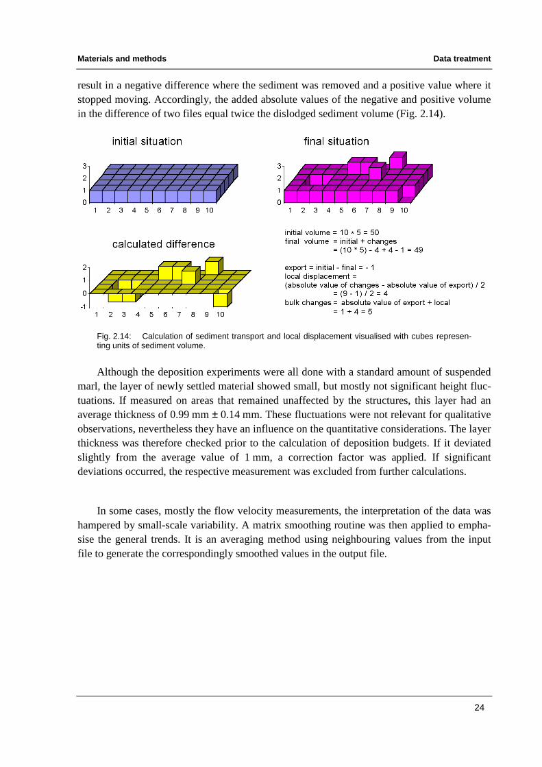
Materials and method s Data treatment
24
result in a negative difference where the sediment was removed and a positive value where itstopped moving. Accordingly, the added absolute values of the negative and positive volumein the difference of two files equal twice the dislodged sediment volume (Fig. 2.14).
Fig. 2.14: Calculation of sediment transport and local displacement visualised with cubes represen-ting units of sediment volume.
Although the deposition experiments were all done with a standard amount of suspendedmarl, the layer of newly settled material showed small , but mostly not significant height fluc-tuations. If measured on areas that remained unaffected by the structures, this layer had anaverage thickness of 0.99 mm ± 0.14 mm. These fluctuations were not relevant for qualitativeobservations, nevertheless they have an influence on the quantitative considerations. The layerthickness was therefore checked prior to the calculation of deposition budgets. If it deviatedslightly from the average value of 1 mm, a correction factor was applied. If significantdeviations occurred, the respective measurement was excluded from further calculations.
In some cases, mostly the flow velocity measurements, the interpretation of the data washampered by small -scale variabili ty. A matrix smoothing routine was then applied to empha-sise the general trends. It is an averaging method using neighbouring values from the inputfile to generate the correspondingly smoothed values in the output file.

Results Control measurements
25
3 Results
3.1 Control measurements
The near-bottom velocity gradient of the boundary layer was present over a flat flumebed covered with sand at both flow velocity settings. The average free-stream velocity was1.7 cm s-1 for the slow flow and 10.2 cm s-1 in the faster flow conditions. The correspondingshear velocities were 0.12 and 0.63 cm s-1, the roughness lengths were 87 and 12 µmrespectively. Reynolds stress values in the free-stream region were an order of magnitudehigher at the faster speed than at the slow speed, i.e. 0.0031 N m-2 instead of 0.00034 N m-2.The horizontal, cross-stream and longitudinal planar section flow measurements all showed auniform velocity distribution of the main horizontal flow component (U) throughout the testsection, independently of the selected flow speed. However, a slight clockwise cross-streamdeviation (ca. 4% of the incoming flow speed) was found. The longitudinal (x,z) sections canalso be analysed as series of successive vertical profiles measured along a streamwise line.They thus complement the high resolution vertical profiles measured separately, bothdisplaying the bottom boundary layer gradient (Fig. 3.1).
Fig. 3.1: Longitudinal section through the test section centre line in the flume channel. Left :measured at 2 cm s-1, Right: at 10 cm s-1. Both graphs show relative flow velocities U/Umax, the ratio offlow speed at a position (x,z) to the free-stream value. A vertical velocity profile is inserted in eachgraph; the values were extracted from the corresponding data set. The arrows indicate strength andangle of the vector UW.
The roughness length (z0) is a measure of the downstream propagation of f low distur-bances caused by roughness elements. In the case of the flat and smooth control surface, z0
did not change though (Fig. 3.2). These values were extracted from the (x,z) longitudinalsection data. The mean roughness length was 0.19 ± 0.04 mm.

Results Control measurements
26
Fig. 3.2: Roughness length z0 extracted from the x,z longitudinal section at 2 cm s-1. a): plot of thesuccessive vertical profiles comprised in the file. b): magnified plot of z0 above of the sediment surface.
Repeated erosion experiments resulted in an average erosion threshold value Ucrit of22.5 cm s-1, i.e. a shear velocity of 1.3 cm s-1 for the sand. The deposition experiment ended inan evenly distributed coating layer of deposed material (Fig. 3.3). The thickness of this layerwas 0.99 ± 0.14 mm, i.e. a total deposition of 11.4 cm3 on the tested area (135 cm2). The area-related deposition was 846 cm3 m-2.
Fig. 3.3: Thickness of the deposed marl layer in the control experiment. The dots symbolise cross-stream average height values (n=46 per dot).

Results Soli tary biogenic s tructure effects
27
3.2 Soli tary biogenic s tructure effects
3.2.1 Flow regime around the structures
Tested at 2 and 10 cm s-1, the flow regime was significantly influenced by the protrudingsolitary structures (worm tube, snail , mussel and sand mound), whereas the depressions onlyhad a low impact on the overlying flow (pit and track). The longitudinal (x,z) planar flow sec-tions of the latter structures showed no remarkable changes of the horizontal main flow com-ponent U (Fig. 3.5). The bottom boundary layer remained unaffected in these two layouts, andthe water within the depressions was merely stagnant.
In contrast, the slender cylinder of the worm tube mimic considerably reduced the flowspeed throughout the total extent of the (x,z) section. The horizontal water motion was sloweddown by more than 50% in a region adjacent to the tube on its upstream side. A wake regionwas formed on the downstream side, with a flow reduction of more than 20%. The wake ef-fects gradually dissipated with downstream distance. The most remarkable effect of this cy-lindrical structure was the presence of a large spot above the tip of the tube, where the hori-zontal flow component U not only dropped to zero, but even was reversed - a strong indicatorof vortex formation (Fig. 3.4, left). The snail , mussel and sand mound layout producedcomparable effects on the main flow vector U. These structures were surrounded by a regionof reduced flow velocities, with a spot of reversed flow on both, the upstream and down-stream side (Fig. 3.4, centre). Unlike the tube, the boundary layer gradient was not disrupted,but compressed instead (Fig. 3.5). The narrowing velocity contour lines indicate a steepergradient, above which the main flow was accelerated to a maximum of 109% of the free-stream velocity. The chosen flow velocity, i.e. 2 or 10 cm s-1, had no apparent influence onthe effects observed in these experiments.
Fig. 3.4: Magnified details showing the various effects of the solitary structures on the main flowcomponent U (colour-coded as relative flow speed U/Umax) in longitudinal (x,z) measurements. Left:region of reversed flow above the tip of the tube. Centre: reversed flow on the sediment surface in thewake of the snail shell. Right: the cross-stream track showed no significant effects. The grey surfacesindicate the position of the respective structures, the white arrows show strength and angle of thevector UW (the vertical flow W values were multiplied by a factor of two for visualisation purposes).

Results Soli tary biogenic s tructure effects
28
Fig. 3.5: Main flow component U in longitudinal sections through the solitary structures. a): 2 cm s-1,b): 10 cm s-1. Worm tube (left) and snail (right) are shown in the top row, mussel (left) and sand mound(right) are in the central row, track (left) and pit (right) in the bottom row. The grey structure shapes arebased on relief measurements. As the sensors cannot measure through the snail shell, the hatchedregion has no data. The contour lines and colours define relative speeds, normalised with the free-stream velocity: U/Umax. The arrows indicate the vector UW strength and angle (the vertical flowcomponent W was multiplied by a factor of two for visualisation purposes).

Results Soli tary biogenic s tructure effects
29
The effects observed for the main flow vector were confirmed by the roughness lengthdistribution (z0) found in the longitudinal planar sections (Fig. 3.6). For the track and pit, thez0 curve connected the upstream and downstream slope in a relatively straight way. It droppedto only 29% (track) or 45% (pit) of the maximum depth of the depressions and thus formedthe upper limit of an unmoved water body inside the depressions. Among the protrudingstructures, snail , mussel and mound affected the surrounding flow in a region downstreamand, to a lesser degree, also upstream of their body. The maximum z0 values were between57% and 78% of the structure height. The tube however raised z0 to a maximum height whichwas 21% above the tube tip, probably a consequence of the turbulent spot found there.
Fig. 3.6: Roughness length distribution around the solitary structures. The values were extractedfrom longitudinal planar section (x,z) flow measurements.
Although snail , mussel and mound induced similar effects on the main flow component, acloser look at the vertical component W nevertheless revealed some differences (Fig. 3.7).The general trend was a flow deflection above the structures, marked by positive values of Won the upstream side and negative values on the downstream side of the bodies. These verticalflows reached more than 10% of the free-stream flow speed in local peaks. Unlike the snail ,both mussel and mound induced a second region of downward flow ahead of the structures,near the sediment surface. This effect was also present - and strongest - in the tube layout,where it occurred along the entire upstream side of the structure. It was balanced by a strongupward flow component in the wake region of the tube. Several isolated spots with strongvertical components may also indicate the presence of either single vortices or of a vortexstreet. The depression structures, namely the track and pit, only caused a minor negative de-flection towards the sediment surface, but no upward motion.

Results Soli tary biogenic s tructure effects
30
Fig. 3.7: Vertical flow component W in longitudinal sections through the solitary structures,measured at a main flow speed U of 2 cm s-1. Worm tube (left) and snail (right) are shown in the toprow, mussel (left) and sand mound (right) are in the central row, track (left) and pit (right) in the bottomrow. The grey structure shapes are based on relief measurements, and the hatched region below thesnail shell has no data. The contour lines and colours define relative speeds, normalised with the free-stream velocity: W/Umax. Blue shades indicate flow away from the bed, red shades symbolisedownward motion. The arrows show strength and angle of the vector UW (the vertical flow W wasamplified by a factor of 2 for visualisation purposes).
A vertical flow deflection and a cross-stream component (V) were also found in the hori-zontal planar (x,y) measurements. Fig. 3.8 shows three differing examples of these results(worm, snail and pit). As seen in the longitudinal sections, the protruding structures caused avertical flow deflection above their apical region. The lateral deflection displayed a similartrend: the flow was diverging ahead of the obstacles and converging again behind them, withlocal peaks of up to 20% of the main flow speed U. Within a kind of "inner region" adjacentto the body and near the bed, worm tube, mussel and mound induced a secondary verticaldeflection that was opposed to the general one in the outer region. The incoming flow wasdirected towards the sediment along the upstream side of the structures and rose again behindthem. This effect was not found in the snail l ayout. The track and pit had no lateral effects andonly a reduced vertical component (W/Umax less than 6%).
The planar flow measurements can thus be summarised as follows: unlike the depressionswith their low impact on the surrounding flow, the protruding structures caused importantvertical and lateral deflections. Some of the structures displayed a reversed vertical flow in aninner region directly adjacent to their bodies, inducing downward motion on their upstreamface, balanced by upward flows on their downstream side. The formation of vortices is highlyprobable, but not yet confirmed by these experiments.

Results Soli tary biogenic s tructure effects
31
Fig. 3.8: Left : cross-stream (V) and right: vertical (W) flow component, measured in planar (x,y)horizons at a main flow speed U of 2 cm s-1 (from left to right). The graphs were blanked out atintersections with the respective structure (top: tube, centre: snail, bottom: pit). The measurementheight was 5 mm for the tube and pit, and 20 mm above the sediment surface for the snail. The contourlines and colours define relative speeds, normalised with the free-stream velocity. Green shadessymbolise a clockwise deflection (V), blue shades indicate vertical flows away from the bed (W).
The vertical velocity profiles measured around the solitary structures basically supportedthe previous results, but they provided additional turbulence information (Fig. 3.9). Theyshowed how the flow was disturbed in the wake regions downstream of the protruding struc-tures. The profiles taken immediately behind the structures had a considerable vertical dis-placement of the boundary layer origin, confirming the high z0 values found in the longitudi-nal planar measurements. The snail and mussel profiles also displayed a relative acceleration(above their apex) between the slow and fast flowing layout.
The Reynolds stress -ρ[U'W'] is a measure of the turbulence level. It was calculated fromthe velocity fluctuations found at each height increment of the vertical velocity profiles. It wasstrongest in the snail l ayout, but pronounced stress peaks were also present in the wake regionbehind the other protruding structures, i.e. worm tube, mussel and mound. These peaks oc-curred mainly at heights where the main flow component U was reduced while the verticalflow component displayed significant deviations from zero, either positive (mussel) or nega-tive (tube, snail and mound). The averaged maximum stress peak height at 1 cm behind the
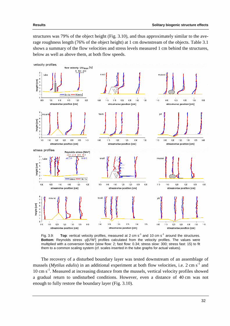
Results Soli tary biogenic s tructure effects
32
structures was 79% of the object height (Fig. 3.10), and thus approximately similar to the ave-rage roughness length (76% of the object height) at 1 cm downstream of the objects. Table 3.1shows a summary of the flow velocities and stress levels measured 1 cm behind the structures,below as well as above them, at both flow speeds.
Fig. 3.9: Top : vertical velocity profiles, measured at 2 cm s-1 and 10 cm s-1 around the structures.Bottom: Reynolds stress -ρ[U'W'] profiles calculated from the velocity profiles. The values weremultiplied with a conversion factor (slow flow: 2; fast flow: 0.34; stress slow: 300; stress fast: 15) to fitthem to a common scaling system (cf. scales inserted in the tube graphs for actual values).
The recovery of a disturbed boundary layer was tested downstream of an assemblage ofmussels (Mytilus edulis) in an additional experiment at both flow velocities, i.e. 2 cm s-1 and10 cm s-1. Measured at increasing distance from the mussels, vertical velocity profiles showeda gradual return to undisturbed conditions. However, even a distance of 40 cm was notenough to fully restore the boundary layer (Fig. 3.10).

Results Soli tary biogenic s tructure effects
33
Fig. 3.10: Left : Reynolds stress at 10 cm s-1 main flow speed, measured 1 cm downstream of thestructures. The height was normalised with the respective structure height kr. Right: flow recoveryexperiment at 10 cm s-1 main flow speed, showing superimposed vertical velocity profiles measuredwith increasing downstream distance from a mussel (Mytilus edulis) assemblage.
Table 3.1: Summary of the flow velocities and stress levels 1 cm downstream of the structures, atambient flow conditions of 2 and 10 cm s-1, measured below (z = 50% of structure height kr) and abovethe structure. The maximum stress values for each flow condition are highlighted.
2 cm s-1 U/Umax at z/kr=0.5 U/Umax at z=7cm -ρρ[U'W'] peak [N m-2] -ρρ[U'W'] at z=7cm [N m-2]
worm 0.15 1.06 0.0013 -0.0005snail -0.006 1.00 0.0320 0.0012mussel 0.03 0.93 0.0084 -0.0002mound 0.15 1.05 0.0021 -0.0005track 0.24 1.01 0.0013 -0.0005pit 0.26 1.05 0.0004 -0.0006
10 cm s-1 U/Umax at z/kr=0.5 U/Umax at z=7cm -ρρ[U'W'] peak [N m-2] -ρρ[U'W'] at z=7cm [N m-2]
worm 0.05 1.08 0.0728 0.0453snail 0.00 1.05 -0.0862 0.0419mussel 0.09 0.94 -0.0907 0.0009mound 0.33 1.02 0.1980 0.0020track 0.53 1.00 0.0163 0.0138pit 0.18 1.08 0.0138 0.0266
Pictures taken during flow visualisation experiments with potassium permanganate(KMnO4) were used to verify the ADV flow measurements. These experiments widely con-firmed the ADV data (Fig. 3.11). The protruding structures caused two distinct flow interac-tion zones. An outer zone was marked by a rather laminar flow, which was slowly surround-ing the obstacles. The dye on the sediment surface followed the obstacle contours at a dis-tance of about 1 cm away from the structures. It then formed the border of a widening trian-gular patch in the wake region of the structures. The only exception was the snail , where thisdye contour was touching the upstream end of the shell . In contrast, the inner zones had char-acteristic vortices in the regions previously identified as spots with a high probabili ty for ele-vated turbulence levels. A stable horseshoe-shaped vortex pattern was present on the sedimentsurface at the base of the structures, extending from their upstream face to the rear sides. This

Results Soli tary biogenic s tructure effects
34
pattern blended into a large vertical circulation cell , li fting from the sediment along thebackside of the structures. Vortices were also detaching from the apical end of the structures.The track and pit merely trapped the coloured water inside their craters, releasing not morethan occasional streaks, although they were eventually swept clean after a strong increase ofthe flow speed. At this higher flow speed, aggregates of combined sand grains and dye wereresuspended on the downstream side of the worm tube.
Fig. 3.11: Flow visualisation experiments with potassium permanganate (KMnO4) dye. The top rowshows a separation line between turbulent effects in the structure-adjacent inner zone and themoderate deflection in the outer zone. Row two and three show the turbulent patterns and vorticeswithin the inner zone. The track and pit in the lowest row had only little influence on the flow regime.

Results Soli tary biogenic s tructure effects
35
3.2.2 Soli tary structure erosion experiments
The erosion experiments with the set of six solitary structures can be divided into twodistinct categories: the flow interaction of the solid structures caused erosion of the surround-ing sediment, whereas the sand structures primarily were reshaped. The worm tube, snail andmussel experiment therefore showed comparable results in the relief scans recorded after 60minutes at 20 cm s-1. A furrow was formed in a horseshoe-shaped region around the upstreamface and at both sides of the structures (Fig. 3.12). This furrow continued farther downstreamfor about 4-5 cm, but gradually became wider and shallower, followed by a couple of troughs.A sand crest appeared between the two furrow fringes in the downstream prolongation of thestructure and extended towards the end of the scanned area. It was created by a fraction of theeroding sediment which only was moved over a short distance within the scanned area (Fig.3.13). The erosion patterns however were not identical. For the worm tube, it was rather a pitaround the tube than a furrow and the crest was triangular. The highest point of the crest wassituated at its downstream end. The crest slopes abruptly ended in a pronounced swallow tail -li ke brink point. The erosion patterns of snail and mussel were almost identical. Their crestshad a peak adjacent to the rear sides of the structure and smoothed out with increasingdistance. Although it was a sand structure, the mound had the same pattern in its wake regionas the rigid structures. Yet, the horseshoe-shaped furrow was missing. The mound itself wasnot swept away, but remained present. It was just elongated into a tetrahedrical shape, resem-bling the triangular crest behind the worm tube. Ridges occurred on the mound slightly down-stream of its widest part, which is the region where flow separation is most likely to happen.The cross-stream track looked like a migrating sand ripple. Its front slope was almost verticaland the rear slope rather gentle, but ending in a second steep zone. The pit only showed anegligible change of its length.
A subtraction of the initial relief scans from those obtained after the flow exposition wasused to locate and to quantify the sediment transport (Fig. 3.14). Values around zero indicateunchanged sediment heights; negative and positive values denote erosion losses or addeddeposition respectively. This method showed that the erosion patterns described in the pre-ceding paragraph were due to a combination of local abrasion and redeposition rather than asimple cause of varying erosion export intensities. A considerable share of the mobile sedi-ment fraction (27-93%) remained within the neighbourhood of the structure. The furrows anddownstream troughs around worm tube, snail and mound were regions of strong erosion, withsediment levels below the ones of the initial layout. The crests however were formed bysediment accumulation; their final height exceeded its initial value. For the sand structures,sediment was dislodged from their exposed surfaces to more sheltered regions like the rearslope of the mound. A secondary region of erosion was found behind the crest peak in mostexperiments, either in the troughs and prolonged furrows (snail , mussel, mound), or at thedownstream end of the worm and track layout. The only exception to this was the pit, whichonly had a moderate transport from its exposed slope towards the subsequent flat surface.

Results Soli tary biogenic s tructure effects
36
Fig. 3.12: Bottom relief measured after 60 minutes exposition to 20 cm s-1 in the erosionexperiments. The flow direction was left to right. Top row: worm (left) and snail (right), central row:mussel (left) and sand mound (right), bottom row: track (left) and pit (right). Isobath lines were addedin the track and pit graph to facilitate the recognition of the structures. The rigid structures (worm, snailand mussel) caused erosion of the surrounding sediment, whereas the sand structures were reshaped.
Fig. 3.13: Side-view of the erosion along the centreline of each solitary structure, extracted from thebottom relief scans, comparing the initial flat sediment with the status after 60 minutes of exposition to20 cm s-1. This figure shows where erosion occurred and indicates that a fraction of the sediment wasonly shifted from one side to the other during the transport process.

Results Soli tary biogenic s tructure effects
37
Fig. 3.14: Differential erosion graphs: bottom scans measured after 60 minutes exposition to flow of20 cm s-1 subtracted from the respective initial stages. Grey zones: unchanged surface, red: sedimenterosion (loss), blue: deposition (gain). The complete surroundings of the mound were affected byerosion, presumably an artefact, and the lowest red shade was therefore replaced by a darker grey.
Due to the remarkable shape obtained after the sand mound erosion experiment, the flowvelocity distribution (set to 10 cm s-1) was measured again in a horizontal (x,y) plane at 5 mmheight above the bed. The results were normalised with the incoming free-stream velocity. Adirect comparison to the flow values obtained from the initial shape (Fig. 3.15) revealed someobvious differences. The main flow component showed a conical wake region with a pro-nounced zone of reversed flow for the initial mound. In contrast, the wake outline was almostlinear behind the new shape and the flow reversal was not detected there. Instead, it hadstronger effects on its upstream side. The cross-stream deflection was weaker around theeroded mound, both for its flow speeds and for the size of the patches. A zone of increasedcross-stream flow was attached to each of the lateral edges of the newly formed tetrahedron,but the wake region was nearly unaffected. The vertical deflection also showed a reducedstrength and the affected zone was narrower in the wake of the eroded shape. However, theupli ft in front of this mound was larger and stronger than upstream of the initial mound.
As the erosion experiments were sequences of relief measurements, repeated after de-fined time intervals, the progress of the erosion process was documented for each structure(Fig. 3.16). It was thus possible to quantify both, the bulk erosion export from the scannedarea and the local sediment displacement, for each interval. The highest transport rates wereusually found immediately after the experiment start for the export and within the first 10minutes for the local displacement (export: up to 395 cm3 m-2 min-1, local: 82 cm3 m-2 min-1).
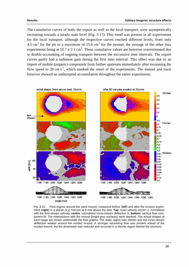
Results Soli tary biogenic s tructure effects
38
The cumulative curves of both, the export as well as the local transport, were asymptoticallyincreasing towards a steady state level (Fig. 3.17). This trend was present in all experimentsfor the local transport, although the respective curves reached different levels, from only4.5 cm3 for the pit to a maximum of 25.6 cm3 for the mound, the average of the other fourexperiments being at 10.7 ± 2.1 cm3. These cumulative values are however overestimated dueto double-accounting of ongoing transport between the successive time intervals. The exportcurves partly had a sediment gain during the first time interval. This effect was due to animport of mobile (organic) compounds from farther upstream immediately after increasing theflow speed to 20 cm s-1, which marked the onset of the experiments. The mussel and trackhowever showed an undisrupted accumulation throughout the entire experiments.
Fig. 3.15: Flow regime around the sand mound, measured before (left ) and after the erosion experi-ment (right) in a planar (x,y) horizon at 5 mm above the bed. Top: main velocity vector U, normalisedwith the free-stream velocity, centre: normalised cross-stream deflection V, bottom: vertical flow com-ponent W. The intersections with the mound (bright grey surfaces) were blanked. The actual shapes ateach stage are shown underneath the flow graphs. The wake region was shorter and the cross-streamdeflection weaker around the eroded mound. A stronger ascending flow was present ahead of theeroded mound, but the downwash was reduced and occurred in a shorter region behind the structure.

Results Soli tary biogenic s tructure effects
39
Fig. 3.16: Erosion sequence of the worm tube layout. The graphs on the right, representing thedifferences calculated from the respective graphs in the left and central column, show where sedimenttransport occurred during that interval.
Fig. 3.17: Bulk erosion export and local displacement sequences calculated for each of the solitarystructures. The strong changes of the export values for the mussel and mound layout during the firsttime interval presumably were artefacts and were thus corrected.

Results Soli tary biogenic s tructure effects
40
The local transport, calculated from the difference between initial and final stages(60 minutes) of the experiments, ranged from 2.3 cm3 for the pit to 8.4 cm3 for the track (ave-rage: 4.6 ± 2.1 cm3 ). In contrast, the bulk export showed a high variabili ty. Values rangedfrom 1.5-1.9 cm3 sediment accumulation (pit and mussel respectively) to 0.6-3.3 cm3 lossesfor track and snail , and to high losses of 10.1 and 10.7 cm3 for worm and mound. The cumu-lated sediment export thus seemed to depend more on structure shape and size than the localdisplacement.
3.2.3 Soli tary structure deposition experiments
As the laser system is an optical method and does not work in turbid water, bottom scanswere thus only available before the addition of the suspended sediment and after it had com-pletely settled out at a flow speed of 5 cm s-1. Alike the erosion experiments, these two stageswere subtracted to identify the location and quantity of the sediment deposition (Fig. 3.18).Again, the four protruding structures had different effects than the two depressions. Wormtube, snail , mussel and mound all had a deposition maximum adjacent to the downstream faceof the structure, with a deposit layer thickness between 3.6 and 5.7 mm (mean: 4.3 ± 1.0 mm).These layouts also had regions of increased deposition farther upstream in the line of thestructures and laterally along their downstream sides. In contrast, the wake region and theimmediate neighbourhood upstream of and on both sides of the structures remained at thesame height as the control experiment. A layer of up to 4.0 mm accumulated beneath the up-stream edge of the pit. The track however showed a rather different effect: it was deeplyburied under a deposit layer of 7.4-18.4 mm. The total deposition in these experiments rangedfrom 12.3 cm3 (pit) to 28.3 cm3 (track), i.e. 914 cm3 m-2 for the pit and 2096 cm3 m-2 for thetrack layout (values based on the 135 cm2 scanned area). If the track result is excluded, theaverage deposition value was 966 ± 47 cm3 m-2. The quantity of deposed matter thus ex-ceeded the control value in all l ayouts.
Table 3.2 shows a summary of the sediment transport results obtained for the solitarystructures. The exact duration of the deposition experiments was not measured, because theconcentration of a defined amount of suspended matter asymptotically decreases with time. Itwas therefore not possible to determine the exact end of these experiments. Repeated tests ofthe optical properties however indicated a duration of 48 hours. The deposition ratescalculated with this assumption remained about one order of magnitude below the erosionrates, with a value of 0.73 cm3 m-2 min-1 for the track and 0.34 ± 0.02 cm3 m-2 min-1 for theother structures. In comparison, the average of all erosion experiments was a transport rate of5.6 ± 4.4 cm3 m-2 min-1.

Results Soli tary biogenic s tructure effects
41
Fig. 3.18: Differential deposition graphs: the bottom scans measured after 2 days at 5 cm s-1 weresubtracted from the respective initial stages. Grey zones: deposition equals the control run, red:sediment losses, blue: enhanced deposition.
Table 3.2: Solitary structure erosion and deposition results. Static results are shown in the top partand transport rates in the lower part of the table. The term "peak rate" refers to the highest valuesfound for a single time interval, the "60' rates" are the transport rates obtained after 60 minutes. Thedeposition rates are shown although the exact duration of the settling process was not measured. Adelay of two days was thus assumed for the calculations. All values were arbitrarily based on the sizeof the scanned surface, i.e. 135 cm2. For the export, negative values indicate losses; positive valuesdenote a net sediment gain.
erosion export[cm3 m-2]
local transport[cm3 m-2]
deposition[cm3 m-2]
deposition minuscontrol [cm3 m-2]
worm -746 324 1028 182snail -201 369 983 137mussel 64 124 924 79mound -796 293 981 135track -42 625 2096 1251pit 116 179 914 68
export peak rate[cm3 m-2 min-1]
local peak rate[cm3 m-2 min-1]
export 60' rate[cm3 m-2 min-1]
local 60' rate[cm3 m-2 min-1]
Deposition rate[cm3 m-2 min-1]
worm -248 45 -12.43 5.40 0.36snail -8 47 -4.03 7.39 0.34mussel 30 10 1.06 2.07 0.32mound -395 78 -13.27 4.89 0.34track -168 82 -0.70 10.41 0.73pit -33 5 1.93 2.98 0.32

Results Roughn ess density effects
42
3.3 Roug hness density effects
3.3.1 Flow interactions
The effects of increasing roughness densities RD (percentage of the bed covered bystructures) were examined. This was done with a modified worm tube layout, where varyingnumbers of tube mimics were arranged in an equidistant and staggered pattern. Planar hori-zontal flow measurements performed in previous studies with comparable layouts (Friedrichs,1996; Friedrichs et al., 2000) were refined here and complemented by new data. Flow velocitychanges were measured in longitudinal planar (x,z) sections along a tube-free line through thearray. The lowest density, RD 0.6%, had no overall effects on the main flow vector U, excepta slight flow acceleration above the downstream end of the tube array. The roughness lengthz0 also did not change considerably: it was 0.43 mm upstream of the tubes, 0.40 mm betweenthem and 0.62 mm at their downstream end (Fig. 3.19). In contrast, RD 1.7% and 3.9%showed an increasing flow interaction. At RD 1.7%, the flow speed gradually was reducedtowards the rear end of the tube array. This effect started at the tube tips at about halfwaythrough the tubes and extended down to the sediment surface at the rear end, where U wasreduced to 55%± 6.8%. The roughness length was 0.81 mm, 4.64 mm and 16.70 mm at theupstream edge, centre and downstream of the tube array respectively. At RD 3.9%, z0 wasaround 23 mm throughout the tube assemblage, and 15.53 mm in the wake zone. Accordingly,the flow speed U was reduced to 32% ± 20.4% inside and 47 ± 21.98% downstream of thetubes. The flow speed was strongly reduced around the tube tips (20% ± 12.7%).
Fig. 3.19: Flow velocity effects induced by increasing roughness densities RD of 0.6% (top), 1.7%(centre) and 3.9% (bottom). Left : longitudinal (x,z) sections of the normalised main flow componentU/Umax. The arrows indicate strength and angle of the vector UW and the grey boxes represent theworm tubes. Right: roughness length z0 values extracted from the sections on the left. Flow speedswere gradually reduced with increasing roughness densities.

Results Roughn ess density effects
43
The vertical flow vector W showed a pronounced upward component in all three layouts(RD 0.6, 1.7 and 3.9%). Highest values were found on the upstream end, above the tips of thefirst row of tubes (Fig. 3.20). These vertical flows were ranging between 10% of the free-stream flow speed U∞ for RD 0.6% and 23% for RD 3.9%. Alike the main flow vector U, thevertical flow component was gradually stopped with increasing roughness density, until thestagnation zone covered the total tube array. Small patches of negative values, i.e. flow to-wards the sediment surface, were present in the wake zones of all three layouts.
Fig. 3.20: Influence of increasing roughness densities RD of 0.6% (top), 1.7% (centre) and 3.9%(bottom) on the relative vertical flow velocity W/Umax. The arrows indicate strength and angle of thevector UW and the grey boxes represent the worm tubes. The strength of the vertical deflection waspositively correlated with the roughness density, and the water between the tubes gradually becamestagnant.
3.3.2 Roughn ess density-related sediment t ransport
In the erosion experiments, the basic transport pattern was similar to the one described forthe solitary worm tube. The sediment was swept away on the tube base and partly redeposedfarther downstream. At the lowest roughness density of RD 0.6%, these successive pits andcrests were formed throughout the tube array (Fig. 3.21). However, increasing roughness den-sities led to a gradual overlapping of the regions affected by each individual tube. The sedi-ment transport therefore shifted from repeated local effects towards a singular large-scalepattern. In addition, the pit-to-crest distance shortened progressively. At roughness densitiesof RD 3.9% and 7.7%, the sand was only moved within the first rows of tubes, leaving theremaining parts of the array unaffected. So, 54.0% of the total array was affected by erosion atRD 0.6% but only 42.1% of the area at RD 3.9%.

Results Roughn ess density effects
44
Fig. 3.21: Erosion experiments with increasing roughness densities RD. a): differential erosion plots(final minus initial relief). The yellow lines indicate the limits of the tube arrays, the yellow dots locateweak data points (mainly the structure shadows). b): transport magnitudes. The control and solitarytube values were added. Due to a high number of weak data points for RD 7.7%, the local transportvalue was excluded, whereas the export value appeared to match the hypothetical trend (solid line).

Results Roughn ess density effects
45
Unfortunately, the tubes at RD 7.7% were too narrow for the laser system to obtain a reli -able data set. The percentage of discarded data points, mainly due to the object shadows, was3.3%, 7.2%, 14.5% and 32.2% for RD 0.6%, 1.7%, 3.9% and 7.7% respectively. TheRD 7.7% results were thus excluded from further data treatment.
The local transport was highest at RD 0.6% with 3232 cm3 m-2 and decreased to627 cm3 m-2 for RD 3.9%. Accordingly, the export trend dropped from a maximum value of2102 cm3 m-2 at RD 1.7% to 998 cm3 m-2 at RD 3.9% and possibly was 207 cm3 m-2 atRD 7.7% (unreliable due to high number of discarded data points in the file). As both trendsconverge against zero, a stabili sing effect can be assumed for high roughness densities. Thisinterpretation was confirmed by the erosion threshold experiments (Fig. 3.22). The averagecritical shear stress of the solitary structures was 0.78 ± 0.09 cm s-1, i.e. 59.4% of the erosionresistance in the control run. The lowest roughness density of RD 0.6% started eroding at0.81 cm s-1 or 61.4% of the control. The values gradually climbed with increasing roughnessdensity. The shift from destabili sing effects to sediment stabili sation occurred betweenRD 1.7% and RD 3.9%. An additional layout with RD 9% exceeded the control value by36%, which was a shear velocity of 1.80 cm s-1.
Fig. 3.22: Critical erosion thresholds of the solitary structures and of increasing roughness elementdensities RD, expressed as critical shear velocity U*crit (red values = percent of control threshold).
The influence of the roughness density on the deposition was tested with worm tubes ofRD 0.6, 1.0%, 1.7% and 3.9% (constant spacing, staggered) and mussel-shaped bodies ofRD 1%, 2%, 4% and 8% (random distribution). Like their solitary counterparts, these struc-tures were surrounded by a region of reduced deposition on their upstream and lateral sides,followed by a crest of enhanced deposition on their downstream sides (Fig. 3.23). With in-creasing roughness densities, the regions of reduced deposition were enlarged until theyoverlapped at RD 3.9% (tubes) and RD 4% (mussels). As a consequence, the regions of en-hanced deposition were moved to the borders of the roughness element arrays, both upstreamand downstream. A deposition layer thickness of more than 1 mm covered 52.6% of the

Results Roughn ess density effects
46
RD 0.6% tube array and 40.7% of the RD 1% mussels, but only 19.7% of the RD 3.9% tubesand 16.8% of the RD 8% mussels. The deposition volume therefore decreased with increasingroughness density and remained below the control value at RD 1.7% or more. The averagefraction of discarded data points was 6.6 ± 2.7% and never exceeded 11%.
Fig. 3.23: Deposition at increasing roughness densities RD. a): differential (x,y) graphs showing thedeposition level for worm tube RD 0.6, 1.0, 1.7 and 3.9% respectively (left) and mussel RD 1, 2, 4 and8% (right). White contours show the position of each structure, yellow lines delimit the tube arrays. b):sediment transport magnitudes measured as a function of roughness density. The grey zone indicatesvalues below the control experiment, i.e. at RD of more than 1.7% (tubes) or 2.0% (mussel). Controland solitary structure values were included, and hypothetical trends were drawn as solid lines.

Results Artificial macrobenthic community
47
Erosion and deposition both were reduced with increasing roughness densities, startingfrom RD values around 2%. At higher RD values, all results showed a considerable reductionof their respective factors (flow velocity, erosion threshold, transport volumes). Table 3.3shows an overview of the sediment transport results of the roughness density experiments.
Table 3.3: Summary of the roughness density-dependent sediment transport results, compared to themean values from the solitary structure experiments. The deposition measured for the bare sandcontrol (846 cm3 m-2) was subtracted in the last column (deposition minus control).
structureRD
erosion export [cm3 m-2]
local transport [cm3 m-2]
deposition[cm3 m-2]
deposition minuscontrol [cm3 m-2]
tubes 0.6 % 1133 3232 848 2tubes 1.0 % 916 70tubes 1.7 % 2102 2209 828 -17tubes 3.9 % 998 627 633 -212mussel 1 % 962 116mussel 2 % 821 -25mussel 4 % 821 -25mussel 8 % 640 -206mean solitary structures 268 319 1154 309
3.4 Artificial macrobenthic community
3.4.1 Flow regime modifications of the community
A natural benthic macrofauna community was artificially reproduced in the flume chan-nel in order to ascertain if the previous results (cf. chapters 3.1-3.3) can be extrapolated tofield conditions. This community (RD 9.6%) consisted of species that were commonly foundin the DYNAS study area. The mimics, representing different polychaete and mollusc species,were randomly distributed on an area of 62 cm length and 18 cm width.
The effects of this layout on the flow regime were measured in three parallel longitudinal(x,z) sections, along cross-stream positions of y=50, 100 and 150 mm respectively (Fig. 3.24).The two lateral ones of these sections included larger structures (mussels and sand mound),whereas the central one only touched short worm tubes. Hence, strongly reduced or reversedflows were mainly found around the large structures in the two peripheral sections. However,the central section also showed these effects. Instead of individual wake regions of the rough-ness elements, they merged into a near-bed layer of very slow flow velocities. This layer, pre-sent in all three sections, was formed near the upstream ends and was gradually enlarged far-ther downstream. The roughness length z0 was 0.18 mm, 2.32 mm and 6.73 mm at the en-trance of the sections at position y=50, 100 and 150 mm respectively. The z0 values at the rearend of these sections were expanded to 3.81 mm, 5.84 mm and 7.08 mm (Fig. 3.25). Theywere thus approximately equal to the heights of the worm tube mimics (5-11 mm), but re-

Results Artificial macrobenthic community
48
mained well below the sizes of the mussel clumps (average height: 20.0 ± 3.4 mm) and of thesand mound (19.1 mm) with only 27.9% of their height.
Fig. 3.24: Flow effects of a flume layout reproducing a natural community. Flow velocities weremeasured along three parallel longitudinal (x,z) sections through the community, at cross-streampositions of y=50, 100 and 150 mm respectively. a): normalised horizontal main flow vector U/Umax, b):vertical flow component W/Umax.
The vertical flow vector W showed the usual deflection above the structures, composedof a succession of pronounced upward and downward motion (Fig. 3.24). This up-and-downpattern was repeated twice in the peripheral sections, due to the presence of the large struc-tures, but remarkably was also detected in the central section despite the absence of corres-ponding structures. Reynolds stress values showed no considerable changes in the slow flowvelocity setting (2 cm s-1), but were increased by an average factor of 7 between the upstream

Results Artificial macrobenthic community
49
ends (mean value: 0.016 ± 0.010 N m-2) and the downstream sides of the sections (meanvalue: 0.111 ± 0.023 N m-2) in the faster flow (10 cm s-1).
Fig. 3.25: Effects of an artificially reproduced natural community on the roughness length z0. Flowvelocities were measured along three parallel longitudinal (x,z) sections through the community, atcross-stream positions of y=50, 100 and 150 mm respectively. Left : roughness length in the centralsection at y=100 mm. Right: roughness length distribution along all three sections.
A flow velocity measurement in a planar horizon at 1 cm above the sediment surface alsoconfirms the dominant impact of the larger structures. All three flow components, U, V andW, displayed changes near the mussel assemblages or the sand mound (Fig. 3.26). Thevertical flow component was directed away from the sediment on the exposed sides of thesestructures and down again on their leeward sides. A general speed reduction trend washowever present in the main flow vector U, gradually slowing down with distance from theleading edge of the community. Its normalised cross-stream average U/Umax decreased from83% to 53% in the first third, and rose from 68% behind the sand mound to 74% at the far endof the array.
3.4.2 Sediment t ransport in the artificial community
The artificial community was also exposed to a flow speed of 20 cm s-1 for 60 minutes inan erosion experiment. The area was then scanned by the laser system (Fig. 3.27a). Additionalphotographs showed that the coupled sediment erosion and redeposition occurred in the sur-roundings of each individual structure in the array, including the smallest worm tubes (Fig.3.27b). However, the most important local height differences were mainly found near thelargest structures, i.e. the mussel groups, the sand mound and the pit adjacent to it. Deephorseshoe-shaped furrows of up to 5.2 mm depth were created in front of the mussel groups.Their counterpart, i.e. the deposition crest, was particularly high on the inner side of thesecond mussel group (4.6 mm at position x=1250, y=150 mm). The sand mound and pit wereboth eroded on their exposed face (2.7 and 7.2 mm loss respectively) and displayed local re-deposition of up to 4.7 mm on their sheltered sides. Some of the large worm tubes (Lagiskoreni-type) also caused erosion of more than 1 mm, especially in a central patch close to thesand mound. In contrast, a few tubes induced the formation of a new mound of 2-3 mm heighton the upstream edge of the array (position x=850, y=50 mm). In total, 74% of the surface

Results Artificial macrobenthic community
50
was affected by erosion losses, 12% by losses of more than 1 mm. Redeposition affected25.7% of the area, and it exceeded 1 mm on 4.7% of the area. The erosion export from thecommunity surface was 352 cm3 m-2 (discarded data points: 3.9%) and the correspondinglocal displacement within the array was 157 cm3 m-2. Expressed as sediment transport rates,this would be an export of 5.87 cm3 m-2 min-1 and 2.62 cm3 m-2 min-1 for the relocation.
Fig. 3.26: Flow effects of an artificially reproduced natural community, measured in planar horizonsat 1 cm above the sediment surface. Top : main flow vector U, normalised with the free-stream velocityUmax. Centre: normalised cross-stream component V/Umax. Bottom: normalised vertical flowcomponent W/Umax. Grey surfaces were intersections with the biogenic structures.
In the deposition experiment, large parts of the total surface (92.2%) were covered by alayer of newly settled material (Fig. 3.28). The overall trend was a slight increase of the layerthickness in along-stream direction through the array, from 0.98 mm (cross-stream average) atthe upstream end to 1.07 mm at the farthest end (Fig. 3.29). However, this increase was notlinear, but patchy. A fraction of 49.8% of the total surface had a layer thickness of more than

Results Artificial macrobenthic community
51
1 mm, i.e. above the control value. The largest of these patches surrounded the sand moundand covered its upstream face, whereas the other high deposition patches had no obvious linkto one of the other major structures. The characteristic accumulation mounds found behind thesolitary structures and at low roughness densities were not present in this layout. The totaldeposition magnitude was 961 cm3 m-2, i.e. 116 cm3 m-2 more than in the control run(discarded data points: 5.9%).
In comparison with the previous roughness density experiments, the erosion test of theartificial community (RD 9.6%) confirms the sediment stabili sing effect, both for the exportand local transport values (352 and 157 cm3 m-2, respectively). In contrast, the deposition wasmuch higher in the community than the corresponding values obtained with arrays of identicalstructures (962 cm3 m-2, i.e. 116 cm3 m-2 more than the control run).
Fig. 3.27: Sediment erosion inside an artificially reproduced benthic community. a): top: reliefscanned after 60 minutes at 20 cm s-1, bottom: height differences obtained after subtraction of the finalsituation from the initial one. Red spots indicate erosion losses, blue shows local deposition. b):pictures of the community taken after the experiment. Left and centre are side-views; right: top view.Flow direction was from left to right in all graphs.
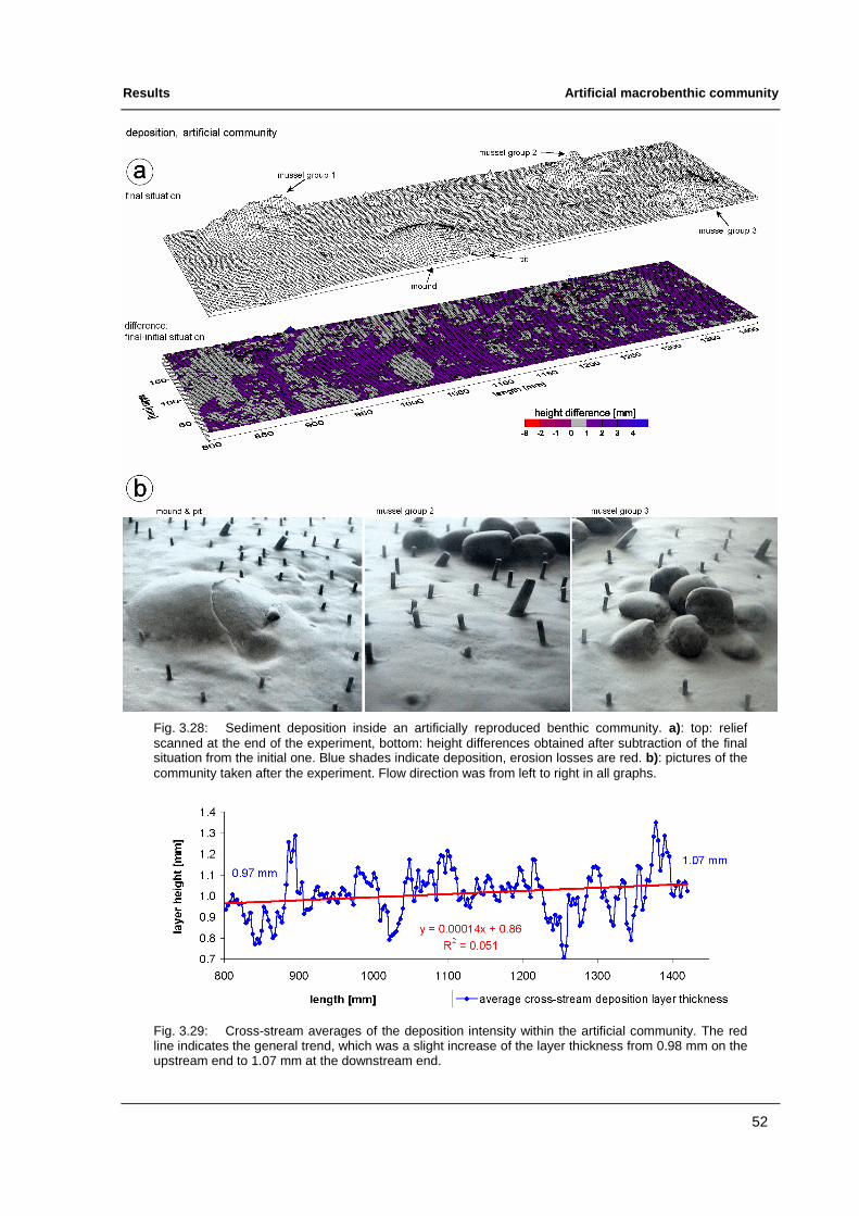
Results Artificial macrobenthic community
52
Fig. 3.28: Sediment deposition inside an artificially reproduced benthic community. a): top: reliefscanned at the end of the experiment, bottom: height differences obtained after subtraction of the finalsituation from the initial one. Blue shades indicate deposition, erosion losses are red. b): pictures of thecommunity taken after the experiment. Flow direction was from left to right in all graphs.
Fig. 3.29: Cross-stream averages of the deposition intensity within the artificial community. The redline indicates the general trend, which was a slight increase of the layer thickness from 0.98 mm on theupstream end to 1.07 mm at the downstream end.

Discuss ion Soli tary structures
53
4 Discuss ion
4.1 Soli tary structures
4.1.1 Near-bed flow around soli tary structures
The flow patterns measured around the protruding solitary structures reflect the observa-tions of f low-obstacle interaction published by several authors (e.g. Carey 1983; Eckmannand Nowell 1984; Abelson et al. 1993; Friedrichs et al. 2000). According to these authors,most of the water diverges laterally around isolated obstacles, whereas only a small fraction isdeflected over their top. The vertical deflection towards the sediment brings water with highermomentum closer to the bed than in an undisturbed boundary layer. A vortex develops on thebase of the obstacle, progressing from the upstream face along both sides and merging with avertical circulation present in the wake of the obstacle. This field was broadly studied in hy-draulic engineering, from first observations like Schlichting (1951) or Hunt et al. (1978) untilrecent works (Ali and Karim, 2000; Graf and Istiarto, 2002; Muzzammil and Gangadhariah,2003). One of the most comprehensive and convincing descriptions is given in Shamloo et al.(2001). With a well -developed boundary layer above a solid surface, pressure gradients forcethis boundary layer to separate when it approaches an obstacle that extends through the vis-cous sublayer. One part of the separated flow surrounds the obstacle at some distance in arather non-turbulent way - although not necessarily laminar, while the other part forms vor-tices when it hits the upstream face of the obstacle. The separation line between these twowater bodies appears in dye-injection experiments as a dark contour on the bed, inside ofwhich the dye is washed away. The velocity outside of the separation line approximatelyequals the free-stream flow. It diverges laterally in front of the obstacle, but also has a strongascending component over the top. In contrast, the horizontal flow is considerably reducedinside of the separation line, where two types of vortices are formed. Horseshoe-vortices aregenerated on the ground and in front of the upstream face of the obstacle. They extend alongits sides and continue downstream into the wake region (Fig. 4.1a). These vortices producehigh bed shear stress that could cause erosion around the obstacle. The second vortex type isarch vortices. They are detaching from the flow separation line of the body and are graduallypushed by a strong downwash behind the obstacle until they come close to the ground. Theenclosed region where these arch vortices occur is called the recirculating region or primarywake. Its downstream end marks the flow reattachment point on the bed. The added verticalflow component induces a local acceleration of the wake flow (Fig. 4.1b) downstream of thereattachment point. The secondary wake outside of the recirculating region tends to roll upinto discrete vortices, but also includes turbulence from the horseshoe and arch vortices. Itextends far downstream of the obstacle, gradually dissipating with increasing distance.

Discuss ion Soli tary structures
54
Fig. 4.1: Flow distribution around an obstacle, showing. a): flow separation, vortex formation andrecirculating region, b): vertical and cross-stream velocity profile changes along the plane of symmetry.Modified, after Shamloo et al. (2001).
Abelson et al. (1993) introduced the slenderness ratio to describe body morphologies(height-to-width ratio). Tall structures deflect most of the fluid laterally, and thus have anenlarged recirculating region. In contrast, wide and shallow structures generate more ascend-ing flow, with a shorter recirculating region due to the increased downwash behind the struc-ture. Vertical velocity profiles would show a deceleration of the flow in front of the body anda speeding over its top, followed by a gradual return to the undisturbed state as far as 20 dia-meters downstream of the obstacle (Shamloo et al, 2001). Shear is considerably reduced in-side the recirculating region. Eckman and Nowell (1984) reported the distribution of f low andshear around a worm tube-like circular cylinder. They showed that fluid from higher in theboundary layer is forced downward on the upstream face of the cylinder by a vertical pressuregradient. This higher momentum fluid forms the horseshoe vortex on the base of the cylinder.An opposite pressure gradient in the wake causes a reversed vertical and horizontal flow. Theskin friction values had a local minimum at some distance upstream of the cylinder, where the

Discuss ion Soli tary structures
55
flow separation resulted in a vertical deflection. A large region of increased shear stress oc-curred within a horseshoe-shaped region around the structure. Another shear minimum alwayswas present within one diameter downstream of the cylinder, but it was longer behind a shorttube, whereas two more lateral minima formed behind a tall tube instead.
Depressions have the opposite effect from protruding bodies (Nowell and Jumars, 1984;Abelson and Denny, 1997). They increase the cross-sectional area through which water flows,slowing it down when it moves over and into the depression. Shear thus is reduced as well . Inanalogy to the effects of protruding structures, the decreasing velocity leads to pressure gradi-ents with a separation line. The flow separates at the upstream edge of the cavity and has areattachment line beneath the downstream edge (Yager et al., 1993). Momentum transferredacross the separation line drives recirculating vortices inside the depression. The flow velocityin this vortex region is reported to be an order of magnitude slower than the free-stream(Abelson and Denny, 1997). The deepest part of a pit, the apex, has a more or less stagnantbody of water with high residence times up to hours (Yager et al., 1993). The vortex insidethe cavity occasionally becomes unstable. The resulting vortex shedding, as well as periodicsweeps that are breaking through the separation line, cause a bulk fluid replacement inside thedepression. Fig. 4.2 shows the effects of f low across a pit.
Fig. 4.2: Flow distribution across a pit-like depression, showing. a): oblique, 3-dimensional view ofthe separation and reattachment lines, b): side view. Based on direct observation and on theory fromYager et al., 1993.
The results presented in chapter 3.2.1 confirm these descriptions. The worm tube was aslender body, reaching high into the incoming bottom boundary layer, which was disrupted bya static vortex above the tube. This vortex was characterised by a local field of reversed flowand increased Reynolds stress values, especially at 10 cm s-1. Isolated vortices were detachingfrom there and travelled downstream, visible as a series of patches with modified horizontaland vertical flow characteristics (U and W). High cross-stream velocities in the planar hori-zontal measurements were signs of a pronounced diverging flow, as expected for slender ob-stacles. In addition, the vertical component, measured in a longitudinal plane (Fig. 3.7), alsoshowed ascending flow ahead of the tube and descending flow behind it. The potassium per-manganate dye experiments revealed a well -defined bed separation line. Inside this line, thevelocity was reduced and the flow was pushed down towards the bed on the upstream face of

Discuss ion Soli tary structures
56
the tube. This effect was reversed in the recirculating region, visible as ascending flow. Thesize of the recirculating wake region was observed in the dye-injection experiment, whichrevealed an elongated vertical, annular circulation pattern (Fig. 3.11). It was also visible fromthe roughness length calculations, since the roughness length z0 is the near-bed limit of themain stream flow. A second region of descending flow was present downstream of the reat-tachment point, as described in Shamloo et al. (2001).
In contrast, the other protruding structures had a lower slenderness ratio. They thereforecaused more ascending and less diverging flow. The roughness length z0 was increased both,upstream and downstream of the structures. Reduced flow speeds and high Reynolds stresseswere indicators for vortex formation in these regions, which was confirmed by the dye ex-periments. Surprisingly, the snail had no descending flow on its upstream face, inside of theseparation line. This may be due to its shape. In fact, a patch of accumulated dye was foundon the bed, touching the frontal edge of the shell . This edge had a short extension that lookedlike a dolphin beak or the bulb-bow of ocean-going ships. With such a streamlined shape, thetypical horseshoe-vortex thus only formed on the lateral sides of the shell . However, all pro-truding structures produced flow effects li ke those described in literature (Shamloo et al.,2001). The water was deflected around the obstacle in an outer region, and typical vorticeswere present inside the separation line on the bed and in the recirculating region.
The depressions, i.e. track and pit, caused no obvious changes of the main flow. Only aweak vertical flow towards the bed was measured. The roughness length values marked theupper limit of the separation line, beneath which the net forward motion was stopped. The dyeexperiment revealed slow vortices inside the cavities. A stagnant layer formed in the deepestpart of the pit, confirming literature descriptions (Yager et al., 1993). A strong increase of thefree-stream velocity was needed to move this water body. Periodic inflow was then observedat the downstream edge of the pit, balanced by a dye streak release on the upstream edge. Thedepressions thus were merely producing sheltered conditions, and only their downstreamedges were exposed to the main flow.
4.1.2 Sediment t ransport processes around the soli tary structures
In chapter 4.1.1, the flow interactions of the solitary biogenic structures were mainlyidentified as local sources of enhanced bed shear for the protruding structures, and reducedshear for the track and pit. These effects are magnified at increased flow speeds, until theygenerate sediment transport. Erosion occurs when the shear stress τ0 of the fluid acting on thebed exceeds the criti cal entrainment stress τcrit of the sediment. The deposition of movingsediment particles depends on the interplay between the settling velocity of particles and theshear stress-related resuspension (Self et al., 1989; Dade et al., 1992). Local erosion and relo-cation can thus occur even at flow speeds below the erosion threshold of the sediment. Acomparison of the flow measurements with the sediment transport experiments shows a goodcorrelation. Regions with important flow effects also were subject to sediment transport.

Discuss ion Soli tary structures
57
Fig. 4.3 shows a superposition of the vertical flow component and of the erosion patternsaround the worm tube, demonstrating their close linkage.
Fig. 4.3: Erosion pattern (top left ) and vertical flow component (top right) around the solitary wormtube, superposed (bottom) to show how they are connected to each other (red contour colours =down, blue = up). The descending flow on the upstream side of the tube caused the scour hole aroundthe tube base, the ascending wake flow in the recirculating region initiated deposition, and the seconddescending flow zone marked the downstream end of the deposition crest at the reattachment point.
Erosion mainly occurred inside the obstacle-induced flow separation lines. This innerzone was marked by the horseshoe-vortices upstream and on the sides of the structure, by thearch vortices and by the recirculating region. These vortices caused characteristic modifica-tions of the bed shear stress, as described in Eckman and Nowell (1984). As a result, a typicalhorseshoe-shaped scour hole appeared around the base of the worm tube and mussel (Grafand Istiarto, 2001; Ansari et al., 2002; Kothyari and Ranga Raju, 2001; Muzzammil andGangadhariah, 2003). The snail also had this scour hole, which however was disrupted infront of its "dolphin beak" extension. Although the mound also produced a vortex (reversedflow on the frontal slope in Fig. 3.5), the gentle slopes have redirected it away from the bed.The scour hole was thus not present around the mound (cf. dye accumulation around themound base in Fig. 3.11). As the mound was made of sediment, it was subject to erosion in-stead. The body separation line, from which eddies were shed and which is the origin of thearch vortices, developed into an erosion crest. The sharp ridge of this crest was formed bydeposition due to a momentum loss of the detaching eddies (Fig. 4.4). Comparable conditionshave reshaped the track and pit. The vertical vortices inside of these cavities have movedsediment particles down along the exposed slope, eroding the upper edge and accumulating

Discuss ion Soli tary structures
58
them inside the cavity. This transport caused the exposed slope to flatten out, an effect whichwas furthermore enhanced by the erosion of the upper edge of this slope, situated above thereattachment line and thus exposed to the main stream.
Fig. 4.4: Planar horizontal measurement (5 mm above the bed) of the cross-stream diverging flowaround the sand mound (left). The detail view shows a local deflection peak, which indicates flowseparation.
Ascending and reversed horizontal flow in the recirculating wake region of the protrudingstructures led to a partial redeposition of the sediment from the scour hole. The worm tubewas surrounded by a scour pit and two parallel troughs in the path of the weakening horseshoevortex. A crest formed between these two troughs, in the vertical wake recirculating pattern.As stated in Abelson et al. (1993), the high slenderness ratio comes with a long recirculatingregion and thus a long crest. Shamloo et al. (2001) tested the deposition behind a cubic bodyand a hemisphere. The cube had a deposition immediately downstream of its body, followedby a scour hole. In contrast, the hemisphere first had a scour hole, and then a depositionmound. This observation is explained with different pathways of the two legs of the horseshoevortex, which are joining directly downstream of the hemisphere, but are deflected furtherdownstream behind the cube. In analogy, the deposition mound behind the worm tube in thepresent work had its peak close to the reattachment point. The steep slope behind this brinkpoint marks the separation line between the recirculating region and the main flow. The strongvertical component caused another scour hole downstream of this reattachment point. Thebody plane of the snail (normal to the flow) was also rather tall and thin. The depositionmound therefore developed downstream of a pair of wake scour holes. The mussel and sandmound were wide and shallow instead. Hence, they had shorter recirculating regions, but thehorseshoe vortex legs joined further downstream because of stronger diverging flows. Theirredeposition mound was directly attached to the structures, and decreasing with distance fromthe flow obstacle.
A distinct wake region was not found downstream of the track and pit, as confirmed bye.g. the undisturbed roughness length (z0) values. They nevertheless both produced aredeposition mound downstream of their cavities. It may simply be due to the settling velocityof the suspended sediment. However, undetected weak flow effects can not be excluded.

Discuss ion Soli tary structures
59
Unlike the erosion processes, the deposition around the protruding structures was strong-est outside of their flow separation lines. Although the dye experiments did not show a clearseparation line around all four structures, the deposition patches appear to have formed alongthese limits. Enhanced deposition was found at some distance upstream of the structures, in aregion where the main flow was slowed down and where the vertical and lateral deflectionbegan. A pair of tangential deposition fields may possibly be attributed to the narrowing re-gion in which the horseshoe vortex rejoins the wake flow (cf. Fig. 3.11, worm tube top view).In addition, deposit mounds occurred within the recirculating wake region, in analogy withthe erosion experiment redeposition. The track and tube also confirmed theory and literaturepredictions, i.e. enhanced deposition inside their cavities due to reduced shear and increasedresidence times of particles trapped below the separation (or stagnation) line.
Recapitulating the local distribution of f low-sediment transport interactions, flow reduc-tion and the resulting deposition mainly occur outside of the separation lines of protrudingsolitary structures, whereas erosion and relocation processes are linked to the turbulent condi-tions inside the near-body flow field (Fig. 4.5). The recirculating wake region is however in-volved in both conditions. This distribution of "active spots" is different for depressions,where a considerable flow reduction below the separation line enhances deposition, due toincreased particle residence times. Erosion is strongest on the upper edge of the exposedslope, which the main stream can wear down because it stays above the separation line.
Fig. 4.5: Sediment transport processes around the solitary mussel structure, showing the erosion(top left ) and deposition (top right) patches. Bottom: superposed erosion and deposition graph. Redshades = sediment transport during erosion experiments (dark = loss, bright = gain), blue = enhanceddeposition. Erosion-related transport at higher flow speeds (20 cm s-1) occurred mainly inside the flowseparation line, whereas enhanced deposition (5 cm s-1) happened outside the separation line.

Discuss ion Soli tary structures
60
The erosion time-series of the solitary structures all showed a common trend, with theirlocal transport converging towards a final state. The erosion rates rapidly reached a peakvalue and then decreased with time (Fig. 4.6). This phenomenon is well -known in sedimentdynamics literature like e.g. a review by Paterson and Black (1999). It is described as surfaceerosion (also called "benign" or type I erosion), and is opposed to mass erosion ("bulk","chronic" or type II). It occurs mostly when the shear stress τ0 exerted by the fluid on the bedonly moderately exceeds the erosion threshold τcrit. Erosion ceases at the point where τ0
equals the bed shear resistance. The flow velocity - and thus the bed shear stress - in the ero-sion experiments was kept below the threshold conditions of the sediment. Transport was thusonly induced around the structures and ended when there was no more erodable material left,or if the latter was outside of the region of increased bed shear. This situation is often called"equili brium conditions" or "dynamic equili brium" in hydraulic engineering publications andresults in a stationary sediment distribution pattern (Shamloo et al., 2001; Sumer et al., 2001;Muzzammil and Gangadhariah, 2003). Gaudio and Marion (2003) reported that conditionsclose to equili brium were achieved after a short time. Accordingly, the erosion time-series inthe present work showed a transport rate peak within the first 10 minutes, followed by a rapiddecrease. The major fraction of the local displacement was completed within 60 minutes inmost of the experiments.
Fig. 4.6: Exponential decay of the export and local transport rates around the solitary structures.
This trend was also found for the bulk sediment export, but it was not evident for all l ay-outs. In contrast to the local displacement, the export was an effective sediment loss from thetest area. While the former process was confined to a rather bedload-like transport over shortdistances, the export fraction must have skipped the surroundings of the respective structure,probably through resuspension. Intermediate stages with temporary deposition outside of thelocal transport region were never found during the time-series, a fact that can only be ex-plained by transport as suspended load. Possible pathways of these particles were observed inthe dye-injection experiments and are known from literature (e.g. Carey, 1983; Eckman andNowell , 1984). The export curves of snail and pit first showed a period of sediment accumu-lation, mussel and track even had an ongoing net sediment accumulation. Such an initial gain

Discuss ion Effects of increasing roughn ess densities
61
can be attributed to a fraction of light-weighted "fluff" particles (Thomsen and Gust, 2000;Löffler et al., 2000; Ziervogel and Bohling, 2003), which were hard to remove from theflume. This fluff is easily resuspended and could have dropped on the sediment surface duringthe still water periods of the bottom scan measurements that were repeated after each timeinterval. The accumulation of track and pit was linked to their reduced shear inside the cavi-ties. The mussel however was a protruding structure. It had a flat and wide body and thusproduced strong cross-stream and vertical deflections. The resulting horizontal flow speedreduction may have helped this deposition, which was always found in four repetitions of thisexperiment. The accumulation around the mussel shape was limited to four lateral regions,located on either side of the streamwise centreline, both upstream and downstream.
4.2 Effects of increasing roughn ess densities
4.2.1 Alterations of the near-bed flow in the presence of roughn ess e lements
The role of increasing numbers of roughness elements on the sediment stabili ty was con-troversially discussed in past publications. These effects were first assumed by authors whotried to explain their data. Rhoads et al. (1978) noticed a higher erosion threshold in the pres-ence of worm tubes, but their experimental design was not appropriate to discriminatebetween possible causes. They however assumed flow detachment at the tube tips to be amajor factor. In return, Eckman et al. (1981) and Luckenbach (1986) found worm tubes todestabili se the sediment at low population densities. Nowell and Church (1979) provided afirst systematic study of the flow effects of "Lego" bricks, 0.9 cm high and 2.6 cm2 in area,with roughness densities ranging from about 0.8% to 13% surface cover. They measured ver-tical velocity profiles between the structures. The profiles were nearly undisturbed at low den-sities, termed as "isolated" or "independent" flow conditions. At intermediate densities around2%, the wakes of the individual structures started interacting, thus called "interacting flow".The highest densities of 8-13% produced a strong flow reduction an the formation of a newboundary layer above the structures. This condition was called "skimming flow" (Fig. 4.7).Flow resistance and turbulence were highest for interacting flow. The turbulence intensityprofiles continuously decreased towards the bed in independent flow, but remained highthroughout the wake region at interacting flow. Skimming flow showed a turbulencemaximum at the height of the structure tops for skimming flow. Butman et al. (1994) reporteda 3-10 fold increase of the turbulent stress over Mytilus edulis mussel beds (estimated RDaround 80%), and Crimaldi et al. (2002) report decreasing Reynolds stresses below a stressmaximum layer, for increasing clam densities.
These findings were verified for artificial worm tube densities by Friedrichs et al. (2000).They reported a switch from destabili sing to stabili sing conditions at 2-4.5% roughness den-sity, and purely skimming flow established at roughness densities around 4.5-8.8% for largetubes (3 cm high and 0.5 cm diameter) and around 0.7-1.0% for small tubes (2 cm by 0.2 cm)(Friedrichs, 1996). The onset of skimming flow thus was not only linked to the roughness

Discuss ion Effects of increasing roughn ess densities
62
density. It was also influenced by the shape of the roughness elements and their extent into theboundary layer. Vogel (1994) proposed to link these flow conditions to the ratio of the objectsspacing to their heights. Skimming flow would then happen if the ratio drops close to one. Inthe present study, this ratio was 2.7, 1.5 and 0.9 for the tube array densities RD 0.6%, 1.7%and 3.9% respectively. The mussel arrays had a height-to-spacing ratio ranging from 10.6 atRD 1% to 2.4 at RD 8%. A rough estimate for the artificial community would be a spacing-to-height ratio around 3.
Fig. 4.7: illustration of the three successive flow regimes, depending on the roughness density.Each structure creates its own flow field in independent flow (top ), interactive flow (middle) ischaracterised by wake interaction, and the roughness elements deflect the stream like a single block inskimming flow (bottom) conditions.
The longitudinal flow measurements at worm tube RD 0.6, 1.7 and 3.9% (Fig. 3.19 and3.20) showed some remarkable aspects that can be used as indicators for the different flowconditions. At RD 0.6%, neither the main flow distribution nor the roughness length z0 wereaffected by the tube array. This is a sign for independent flow. As the measurement was donealong a line between two rows of tubes, wake effects were not visible in these graphs. The RD1.7% layout produced spots of reduced flow over the tops of the tubes. These spots were in-creasing in size with distance through the tube array and eventually merged to a wake regionwith 40-60% flow reduction. The roughness length accordingly was enlarged to a maximumheight close to the one of the tubes in the rear part of the array. It then dropped to about halfthe tube size behind the array. The vertical profiles in Fig. 3.19 were double-bowed, with aminimum at the height of the tube tips. This type of profile was attributed to interactive flow(Fig. 4.7). At RD 3.9%, the flow was reduced to below 40% between the tubes and even tozero around their tips. The roughness length reached the tube length, and the vertical profilesin the rear part of the array thus only had a typical boundary-layer shape above the tubes.

Discuss ion Effects of increasing roughn ess densities
63
These conditions therefore manifest skimming flow. Comparable vertical profile measure-ments were presented by e.g. Crimaldi et al. (2002) for Potamocorbula amurensis clams, byNikora et al. (1998) for the moss Fissidens rigidulus and by Gambi et al. (1990) for canopyflow in Zostera marina seagrass meadows.
The vertical flow component (Fig. 3.20) showed an increasingly ascending tendency athigher roughness densities. Both the spatial extent and the strength of this deflection wereaugmented, combined with a widening body of stagnant water within the tube array. Similarobservations were made by Nepf and Koch (1999) for tube and plant arrays of roughness den-sities between 0.7% and 6.0%. Although their structures were slender, and thus mainly gen-erated cross-stream diverging flows instead of ascending deflections, this lateral flow compo-nent gradually was smoothed out at higher densities. The array then acted like a solid bloc,which in return was relatively flat and wide, i.e. it had a low slenderness ratio. According toAbelson et al. (1993), blunt objects mainly induced ascending flow. Data from flow meas-urements in tube arrays at the NIOO-CEME flume facili ty (Yerseke, the Netherlands;Friedrichs, unpublished data) support this theory. The cross-stream flow component V wasconsiderably dampened at RD 2%, but displayed independent flow conditions at RD 1%.
4.2.2 Sediment t ransport through the roughn ess element arrays
The preceding flow regime considerations were endorsed by the erosion experiments.The sand was uniformly eroded throughout the RD 0.6% array and had a threshold that wasnot only 39% below the one of bare sand, but also identical to the average threshold of thesolitary structures. These are characteristics of independent flow. The next layout also haddestabili sing effects, with a threshold below the control value and an erosion pattern coveringthe whole array surface. However, the erosion shifted from individual tube effects towards acollective transport process, indicating the occurrence of interactive flow conditions. Finally,the sediment within the rear part of the tube array was gradually left unaffected in the erosionexperiments at RD 3.9% and 7.7%. The corresponding threshold values were exceeding thecontrol by 4% and 36% respectively. These conditions thus had a stabili sing effect on thesediment and were bound to be skimming flow. The essential deduction would therefore be toidentify independent and interactive flow conditions as destabili sing effects and skimmingflow to stabili se the sediment (Table 4.1). Boström and Bonsdorff (2000) observed decreasingerosion losses in treatments with artificial seagrass beds of low to moderate densities.Romano et al. (2003) described a considerable current velocity reduction in Enteromorphaintestinalis algal mats, ranging from 18% at a roughness density of 10% to 56% at 60% cover.Coupled with this, sediment erosion was diminished by 60% to 90% in comparison to baresand. Meadows of the seagrass Posidonia oceanica also were reported to reduce particleresuspension in the field (Terrados and Duarte, 2000).
Although the results of the deposition experiments were also influenced by the roughnessdensity, they did not confirm the deposition enhancement commonly found in literature. For

Discuss ion Effects of increasing roughn ess densities
64
example, artificial seagrass shoots have been observed to trap loose sediment and largequantities of drifting algae (Boström and Bonsdorff , 2000). Deposition rates in Enteromorphaintestinalis during a tidal cycle were 48% higher at 60% algal cover than on bare sand(Romano et al., 2003). The annual deposition of carbon in Posidonia oceanica seagrassmeadows was evaluated to be 198 g m-2 yr-1, 72% of which were derived from the seston(Gacia et al., 2002). High abundances of the spionid polychaete Polydora cili ata accumulateda deposit layer of up to 50 cm within 21 days (Daro and Polk, 1973). However, high deposi-tion rates in dense polychaete tube lawns were attributed to active suspension feeding beha-viour instead of passive deposition (Frithsen and Doering, 1986).
In contrast, seagrass leave canopies increase the residence time, and thus enhance thesettling rate of suspended matter (Gambi et al., 1990). Granata et al. (2001) investigated theflow and particle distribution in near-shore seagrass meadows, and found consistently lowparticle concentrations inside the meadows - even during storm conditions. They concludedthat decreased flow speeds and turbulence also imply low mixing and a reduced fluid ex-change. The supply of particle-loaded water thus was low, and the sedimentation conse-quently was diminished.
The results of the deposition experiments in the present work displayed decreasing depo-sition at higher roughness densities, regardless of the structure shape. At low densities, theamount of settled material exceeded the control values, and a high percentage of the surfacewas covered by a layer of more than 1 mm thickness (53% for the RD 0.6% tubes and 41%for the RD 1% mussel shapes). According to Nowell and Church (1979), flow resistance andturbulence were highest for interacting flow, with high turbulence levels throughout the com-plete height of the wake region. This situation has caused the apparently contradictory resultsin the next two layouts (RD 1.0% and 1.7% for the tubes, 2% and 4% for the mussels). Thedeposition rose to a maximum of 962 cm3 m-2 for the RD 1.0% tube array, i.e. 114% of thecontrol value, but only covered 21.5% of the total area. It then dropped back to a value justbelow the control at RD 1.7%, whereas the deposition covered 36.2% of the surface. A simi-larly reversed order of the surface coverage was also found for the mussel shapes at RD 2%and 4%, although the deposition was identical in both layouts. This effect may be due to in-teractive flow conditions, where the stronger turbulent mixing first caused an increased importof suspended matter, but reduced the deposition to the wake region of each structure. Themixing then was lower in the second layout, perhaps even not reaching down to the bed anymore. The import of particles into the array consequently was decreased, whereas the distri-bution affected a larger area. Finally, the deposition was strongly reduced to only 20% and17% of the total surface for the RD 3.9% tubes and RD 8% mussels respectively, and re-mained well below the control value. Assuming particularly calm flow conditions as a reasonfor this lack of deposition, this would be a sign of skimming flow. Table 4.1 gives a summaryof possible interpretations of the flow conditions and sediment stabili ty properties for the dif-ferent roughness densities.
The two highest roughness densities of each layout had almost identical depositionvalues, but differing RD numbers: 821 cm3 m-2 at tube RD 1.7% and 633 cm3 m-2 at tube

Discuss ion Effects of increasing roughn ess densities
65
RD 3.9%; 828 cm3 m-2 at mussel RD 4% and 640 cm3 m-2 at mussel RD 8%. The slendertubes apparently cause a stronger flow reduction at low densities, whereas the mussel floweffects were conform with the results of Nowell and Church (1979) who observed skimmingflow at roughness densities between 8% and 13%. Three commonly-used, simple density-related factors were checked for their abili ty to explain this difference between tube andmussel-shape deposition results. However, neither the roughness density, nor the objectspacing-to-height ratio (Vogel, 1994) or the total exposed object surface (normal to the flow)provided a good correlation, because none of them includes the complex non-linear boundary-layer effects. Promising new approaches in high-resolution numerical modelli ng of f lowsacross Zostera marina eelgrass canopies (Abdelrhman, 2003) or over complex bed topogra-phy (Lane et al., 2002) may become adequate tools in this context.
Table 4.1 Summary of the interpretations of the flow conditions and sediment stability properties forthe different roughness densities. The impact of the vertical flow was difficult to assess, but ascendingflow on 53% of the obstacle-free water body signifies that the complete front region was affected, i.e.deflection of the total stream. For the sediment transport, stabilising effects were assumed when therear part of the array remained unaffected by erosion displacement, or at thresholds above the baresand control value. Deposition below the control was taken as a sign of skimming flow with reducedparticle supply into the array.
legend:
RD = roughness density (% cover of the total surface)
wake flow reduction = ratio of free-stream flow Umax to the flow U in the wake behind the structures
flow W %surface = share of the obstacle-free water body with ascending flow W/Umax exceeding 5%
wake z0 = roughness length inside the rear part of the array (tube height = 2.5 cm)
erosion pattern (destab = destabilising; stab = stabilising; indep = independent flow, inter = interactive flow;skim = skimming), classified according to the presence of either isolated effects, collective effects or noeffects in the rear part of the array
threshold %control = erosion threshold, expressed as percentage of the bare sand control value
deposition test minus control = bare sand control value subtracted from the deposition (cm3 m-2)
deposition %surface = share of the sediment surface in the array affected by deposition exceeding 1 mm

Discuss ion Pass ive effects of an artificial macrobenthic community
66
4.3 Pass ive effects of an artificial macrobenthic community
The flow speed distribution in the artificial macrobenthic community was measured at alower resolution, with positioning increments of 2-3 mm. The resulting data thus mainlyshowed large-scale effects, particularly the flow interaction of the sand mound and musselassemblages (Fig. 4.8). At first sight, the reduction of the flow velocity and the deflections incross-stream and vertical direction indicate the flow effects of these large structures. Therewere however important additional flow changes between those structures. The main flowcomponent U was reduced to less than 80% throughout the array, starting near the front end ofthe sand mound and extending down to the rear end of the horizontal planar measurement.The three longitudinal sections showed ascending flow on a common position in the first partof the array (at position x=1000), independently of the presence of a large structure. Theboundary layer thickness also increased with downstream distance in all three longitudinalsections. The average roughness length in the rear part was 5.6 mm. This corresponds to theaverage tube height in the array, but to only 30% of the mound height.
Fig. 4.8: Side-view picture of the artificial community. The flow direction was left to right.
Dade et al. (2001) proposed a simple empirical formula to estimate the roughness lengthof distributed roughness elements in a natural environment. It is the product of the objectheight, of the surface cover and of a correction constant. The estimate for the present commu-nity would be around 0.6-1.8 mm, depending on the structure height value (mean or maxi-mum). This value is in the same order of magnitude as the measured roughness length, butslightly underestimates it. The discrepancy may be due to the fact that a measured roughnesslength maximum is compared to an estimate of the average value for the total surface.
Although the roughness density of the community was high (RD 9.6%), the flow effectsin the longitudinal sections showed no signs of skimming conditions. If this total roughnessdensity is decomposed into the values for each species, the respective values range betweenRD 3.3% and 5.7% for the sand mound and mussel clusters, and 0.1%-0.4% for the wormtubes. According to the interpretations made in the previous chapter, none of these densitieswould be high enough to create skimming flow. They are rather in the range of interactiveflow conditions. This idea is supported by the increased Reynolds stress at 1.5 cm above thesediment in the rear part of the array. Independent flow conditions are characterised by a tur-bulence maximum on the bed (Nowell and Church, 1979).

Discuss ion Pass ive effects of an artificial macrobenthic community
67
The erosion experiment returned low export and relocation values. They were mainly dueto local transport patterns around the large structures, resembling the ones observed for soli -tary elements. A weak transport was nevertheless also found within the tube fields, particu-larly in the central part of the community. The pictures in Fig. 3.27b showed a complex inter-action of scour holes and deposition zones. Comparable results were reported by Fries et al.(1999) who documented bedload transport and ripple formation at flow speeds below thesediment threshold value, in the presence of elevated densities of biogenic sand mounds.Those mounds were built from sand ejected by the head-down deposit-feeding polychaeteCistenides gouldii , but identical results were also obtained with artificial mounds. The ripplesoccurred at densities above RD 20%, when the sediment that eroded around upstream moundswas deposed between the succeeding downstream mounds and thus fill ed the gaps. Theseripples also were found to migrate and can thus cause considerable sediment transport ratesdespite the fact that this transport originated from weak local erosion effects.
The erosion threshold of the community was not determined, since overlapping local ef-fects in this heterogeneous layout impeded a reliable measurement. The low erosion levelwould however indicate a stabili sing effect and thus an elevated overall threshold value.
The deposition was rather evenly spread over the array and its level was higher than inthe unpopulated control experiment. It is thus assumed that the irregular shape, height andspacing of the roughness elements caused interactive flow and thus a strong mixing,associated with an important supply of particles to the array.
The artificial community layout was the reproduction of a typical species compositionfrom the DYNAS and WISTMAK project area (Powill eit and Peine, pers. comm.). The pres-ent results can thus be used as an estimate for the passive biodeposition and bioresuspensionpotential of the area, under flow conditions below the erosion threshold of the underlyingsediment. Sediment and species distribution maps were created in the course of DYNAS, andthe experimental data will be integrated in a numerical circulation model. Values for theroughness length and sediment transport thresholds are among the most important input forthis model, and already have been tested in various configurations (Harff et al., 2003; Peine,in prep.). Meteorological data are used to compute current velocities and bed shear stresses.Storm events are expected to increase the physical forcing through current and wave action,and thus to drive basin-wide sediment transports (Ritzrau and Graf, 1992; Black and Oldman,1999; Li and Amos, 1999). These transports would however partly still be influenced by thestabili sing effects and the undisrupted deposition capacity of benthic communities. Theerosion threshold experiments showed that a tube lawn covering 9% of the surface increasedthe criti cal shear velocity to 136% compared to bare sand. Higher roughness densities couldraise this value even more and thus reduce the erosion risk. A rough estimate could be anerosion resistance increase by a factor of 1.5 to 3. The biogenic contribution to the sedimenttransport would in return play a major role in calm conditions, i.e. below the erosionthresholds. However, isolated biogenic structures, bioturbation, sediment tracks, biodeposits,

Discuss ion Pass ive effects of an artificial macrobenthic community
68
faeces and protruding sediment surfaces can considerably reduce the erosion threshold andthus destabili se the sediment (Davis, 1993; Graf and Rosenberg, 1997; Fries et al., 1999;Andersen et al., 2002).
Fig. 4.9: Overview of the sediment transport values for erosion (left ) and deposition (right) atincreasing roughness element densities. Values below the control level were highlighted in thedeposition graph. The artificial community showed the highest erosion resistance, combined with ahigh deposition capacity.
The species composition and the conditions used in the present study produced a strongstabili sing effect with local displacement and export values well below those of the highesttube lawn tested (Fig. 4.9). The sediment export (resuspension) during erosion conditionswould reach to 352 m3 km-2, which would be a weight of 952 t km-2 with the density of thesand used for the experiments. In contrast, the deposition ranged above the control value andwas much higher than in the tube lawn and mussel bed experiments, but still remained belowthe mean solitary structure (cf. table 3.3). The deposition accounts for with 962 m3 km-2 or1279 t km-2. A conversion of these quantities into flux rates is problematic, because of theabsence of a steady state in the course of the observed processes (initial erosion peak followedby exponential decay) and due to the diff iculties with the definition of the exact depositionexperiment duration. They can however be useful as estimates of the order of magnitude ofthese transports. The erosion export flux for the artificial community thus was5.87 cm3 m-2 min-1 or 952 g m-2 h-1 and the corresponding deposition was 0.33 cm3 m-2 min-1
or 27 g m-2 h-1.
Thomsen and Jähmlich (1998) calculated total particulate matter (TPM) fluxes over amixed benthic community in the Mecklenburg Bight from water samples obtained with abottom water sampling system (BIOPROBE, Thomsen et al., 1994). They found a net resus-pension of 22-130 mg m-2 h-1 at a near-bed flow velocity of 11 cm s-1 in September 1993 anda deposition of 21-388 mg m-2 h-1 at 3.5 cm s-1 in November 1994. These values were lowerthan the estimates for the artificial community, but this can partly be attributed to lower flowspeeds and to important differences in the composition of both, the suspended matter and thesediment. The sediment probably was cohesive (90% < 63 µm) in Thomsen and Jähmlich(1998) and their suspended matter concentration was around 5-7 mg l-1. Turnewitsch and Graf(2003) even measured TPM values around 1 mg l-1 in the same area in July 2001. In thepresent flume study, the median sediment grain size was 220 µm and the suspended marl(8 µm) had an initial concentration of 280 mg l-1. Yet, the laboratory and field results were

Discuss ion Pass ive effects of an artificial macrobenthic community
69
still comparable, despite the differing experimental conditions and methods. A direct conver-sion of the laboratory data to field conditions however remains delicate. Future work shouldaim at a way to overcome these diff iculties and should include combined erosion and deposi-tion measurements for flow conditions, below and above the sediment erosion threshold alike.
In Thomsen and Jähmlich (1998), the POC deposition rates (POC) ranged between 2.4and 7.7 mg m-2 h-1 in November 1994. In September 1993, the authors measured both, a POCdeposition of up to 9 mg m-2 h-1 and a resuspension of 11 mg m-2 h-1 POC on differentstations. Higher values were found in a field flume study of the transport in the GermanWadden Sea (Sylt-Rømø Basin, Königshafen). Asmus and Asmus (1998) reported a POCresuspension rate of 172 mg m-2 h-1 in the sublittoral part of the area and a deposition rate of56 mg m-2 h-1 in the eulittoral zone. In the eulittoral, the lugworm Arenicola marina sandmounds caused a deposition rate of 55 mg m-2 h-1 and the mussel Mytilus edulis 56 mg m-2 h-1.Under stormy weather conditions, the sublittoral POC resuspension rate increased to268 mg m-2 h-1, whereas the intertidal deposition remained unchanged. The Arenicola deposi-tion was however decreased to 40%, i.e. 22 mg m-2 h-1. A typical POC/TPM ratio for resus-pended matter would be around 10% (Blomqvist and Larsson, 1994; Kerner and Yasseri,1997). In the study area, Jähmlich et al. (1998) and Turnewitsch and Graf (2003) measuredlower ratios of 4.6% and 0.5-2% respectively. Assuming a POC/TPM ratio of 1% for theartificial community data, the measured TPM fluxes would correspond to 9.5 g m-2 h-1 POCerosion and to 0.3 g m-2 h-1 POC deposition. These values are close to the storm fluxes givenby Asmus and Asmus (1998).
Storm events with high near-bottom flow velocities only occur sporadically in theMecklenburg Bight. In total, flow velocities beyond the resuspension threshold of the baresediment are limited in time (a few days per year) and in their spatial extent (around 8% of thetotal surface), as stated in (Bohling and Lemke, 2003; Kuhrts et al., 2003). The species of thestudied community are found on a substantial share of the total surface of these coastal wa-ters. In addition to their active biodeposition and resuspension, the passive contribution to theparticle transport may thus be relatively important. During the predominant calm weatherconditions, passive erosion from the community will mainly be limited to local transport,whereas high deposition fluxes would characterise it as a net sink of particulate matter. Sus-pended matter thus would have shorter residence times in the water column and would betransported over shorter distances than in unpopulated areas. This effect would keep a higherfraction of the organic matter in the shallow waters, where it can efficiently be consumed andrecycled. In an attempt to assess the role of the benthic community for the POC fluxes, Asmusand Asmus (1998) also excluded different dominant components of the community from theircalculations. In their scenario without the mussel Mytilus edulis, the deposition was reducedto 53% and the total resuspension was increased to 126% of the natural situation. Extrapolatedto the Mecklenburg Bight, these results would imply that the export and sedimentation ofPOC to deeper (anoxic) regions of the Baltic Sea would be much stronger and faster in theabsence of the benthic community. During sporadic storm events, the community would still
Discuss ion Conclusions
70
impede sediment erosion and may also persist in its passive deposition effect (Thomsen andFlach, 1997), but it would in addition be expected to act as a source of biodeposits and previ-ously captured fluffy material. Wave action in these shallow waters may also counteract thestabili sing effects of the benthic community. The data nevertheless accentuates the impor-tance of macrozoobenthic populations for the transport of particulate matter in theMecklenburg Bight.
4.4 Conclusions
Biogenic macrozoobenthic structures that are exposed to near-bed flow induce character-istic deflection and turbulence patterns. These flow patterns are associated with local fields ofeither reduced or ampli fied bed shear stresses. Solitary structures therefore produce a localsediment transport in their surroundings. Protruding structures have stronger erosion effects,whereas depressions enhance the deposition of suspended matter. The erosion also revealed tobe a combination of export and of local displacement towards redeposition regions. Solitarystructures hence induce simultaneous stabili sing and destabili sing effects.
The erosion around solitary structures occurred even at flow velocities below the criti calthreshold values of the sediment, and can thus destabili se the sediment. Increasing densities ofthese structures gradually modify the near-bed flow and eventually deflect it around and overthe structure array, producing skimming flow conditions where the flow velocity inside thearray is considerably reduced and the roughness length enlarged. Roughness element densitiescovering less than 2 percent of the total surface cause enhanced deposition and high erosionrates. Polychaete tube-like assemblages shift from sediment destabili sing to stabili singproperties around 4% surface cover. Mussel-li ke bodies appear to extend this criti cal densityto 4-8% cover, although the available data for this specific shape does not permit finalconclusions.
The biogenic structures of a macrozoobenthic community also reduce the flow velocity,but their variable sizes generate microhabitats with local modifications of the mean flow con-ditions. The sediment transport capacity therefore is limited to local spots, whereas the pas-sive particle capture and deposition by far exceeds the values obtained from arrays of wormtubes or mussel-shape layouts of the same density. Such a community thus has a strong stabi-li sing effect, which may also persist at flow speeds above the criti cal erosion value of the sur-rounding sediment.
The studied macrozoobenthic community, which covers a significant part of theMecklenburg Bight, therefore has a major impact on the regional transport of sediments andparticulate matter. It slows down the overall transport through sediment stabili sing effects andincreased residence times of particles in the system, but intensifies the local recirculation.

Reference list
71
5 Reference list
5.1 Personal communications
Bohling B., Baltic Sea Research Institute, Marine Geology Department, Seestr. 15, 18119Rostock Warnemünde
Forster S., Baltic Sea Research Institute, Biological Oceanography Department, Seestr. 15,18119 Rostock Warnemünde
Peine F., Institute of Aquatic Ecology, Marine Biology Department, University of Rostock,Albert-Einstein-Str. 3, 18051 Rostock
Powill eit M., Institute of Aquatic Ecology, Marine Biology Department, University ofRostock, Albert-Einstein-Str. 3, 18051 Rostock
5.2 Manuscripts
Peine, F. Evaluation of macrofauna distribution with the use of a geographical informationsystem (GIS), in preparation. (Marine Ecology Progress Series).
Friedrichs, M. and Graf, G., 2003. Description of a flume channel profilometry tool usinglaser line scans. Aquat. Ecol., accepted.
Jonsson, P. R., van Duren, L. A., Amielh, M., Asmus, R., Aspden, R., Daunys, D., Friedrichs,M., Friend, P. L., Olivier, F., Precht, E., Sauriau, P.-G., Schaaff , E., Widdows, J.,2003. Making water flow: a comparison of the hydrodynamic characteristics of 12different biological flume tanks. Aquat. Ecol., submitted.
Ziervogel, K. and Bohling, B., 2003. Sedimentological parameters and erosion behaviour ofsubmarine coastal sediments in the south-western Baltic Sea. Geo-Mar. Lett., in press.
5.3 References
Abdelrhman, M.A., 2003. Effect of eelgrass Zostera marina canopies on flow and transport.Mar. Ecol. Prog. Ser., 248: 67-83.
Abelson, A. and Denny, M., 1997. Settlement of marine organisms in flow. Annu. Rev. Ecol.Syst., 28: 317-335.

Reference list
72
Abelson, A., Miloh, T. and Loya, Y., 1993. Flow patterns induced by substrata and bodymorphologies of benthic organisms, and their roles in determining availabilit y of foodparticles. Limnol. Oceanogr., 38(6): 1116-1124.
Ali , K.H.M. and Karim, O., 2000. Simulation of f low around piers. J. Hydraul. Res., 40(2):161-174.
Andersen, T.J., Jensen, K.T., Lund-Hansen, L., Mouritsen, K.N. and Pejrup, M., 2002.Enhanced erodibili ty of f ine-grained marine sediments by Hydrobia ulvae. J. Sea Res.,48: 51-58.
Ansari, S.A., Kothyari, U.C. and Raju, K.G.R., 2002. Influence of cohesion on scour aroundbridge piers. J. Hydraul. Res., 40(6): 717-729.
Asmus, R. and Asmus, H., 1998. The role of benthic communities for the material exchangein the Sylt-Roemoe wadden sea. In: C. Gaetje and K. Reise (Editors), OekosystemWattenmeer - Austausch-, Transport- und Stoffumwandlungsprozesse. SpringerVerlag, Berlin, pp. 257-302.
Baas, J.H. and Best, J.L., 2000. Ripple formation induced by biogenic mounds--comment.Mar. Geol., 168: 1-4.
Black, K.P. and Oldman, J.W., 1999. Wave mechanisms responsible for grain sorting andnon-uniform ripple distribution across two moderate-energy, sandy continentalshelves. Mar. Geol., 162(1): 121-132.
Blomqvist, S. and Larsson, U., 1994. Detrital bedrock elements as tracers of settlingresuspended particulate matter in a coastal area of the Baltic Sea. Limnol. Oceanogr.,39(4): 880-896.
Bock, M.J. and Mill er, D.C., 1997. Particle-bound organic matter as a cue for suspensionfeeding in tentaculate polychaetes. J. Exp. Mar. Biol. Ecol., 215(1): 65-80.
Bohling, B. and Lemke, W., 2003. Sedimentologie. In: J. Harff (Editor), DYNAS,Abschlussbericht, Rostock, pp. 13-33.
Boström, C. and Bonsdorff , E., 2000. Zoobenthic community establishment and habitatcomplexity - the importance of seagrass shoot-density, morphology and physicaldisturbance for faunal recruitment. Mar. Ecol. Prog. Ser., 205: 123-138.
Brafield, A.E. and Newell , G.E., 1961. The behaviour of Macoma balthica (L.). J. Mar. Biol.Ass. U.K., 41: 81-87.
Buchanan, J.B., 1984. Sediment analysis. In: N.A. Holme and A.D. McIntyre (Editors),Methods for Study of Marine Benthos. Blackwell Scientific Publications, Oxford,England, pp. 41-65.
Butler, J.B., Lane, S.N., Chandler, J.H. and Porfiri, E., 2002. Through-water close rangedigital photogrammetry in flume and field environments. Photogramm. Rec., 17(99):419-439.

Reference list
73
Butman, C.A., Frechette, M., Geyer, W.R. and Starczak, V.R., 1994. Flume experiments onfood supply to the blue mussel Mytilus edulis L. as a function of boundary-layer flow.Limnol. Oceanogr., 39(7): 1755-1768.
Caldwell , D.R. and Chriss, T.M., 1979. The viscous sublayer at the sea floor. Science,205(14): 1131-1132.
Carey, D.A., 1983. Particle resuspension in the benthic boundary layer induced by flowaround polychaete tubes. Can. J. Fish. Aquat. Sci., 40(suppl. 1): 301-308.
Crimaldi, J.P., Thompson, J.K., Rosman, J.H., Lowe, R.J. and Koseff , J.R., 2002.Hydrodynamics of larval settlement: The influence of turbulent stress events atpotential recruitment sites. Limnol. Oceanogr., 47(4): 1137-1151.
Dade, B.W., Hogg, A.J. and Boudreau, B.P., 2001. Physics of f low above the sediment-waterinterface. In: B.P. Boudreau and B.B. Jørgensen (Editors), The benthic boundarylayer: transport processes and biogeochemistry. Oxford University Press, Oxford, pp.4-43.
Dade, W.B., Nowell , A.R.M. and Jumars, P.A., 1992. Predicting erosion resistance of muds.Mar. Geol., 105(1-4): 285-297.
Daro, M.H. and Polk, P., 1973. The autecology of Polydora cili ata along the Belgian coast.Neth. J. Sea Res., 6: 1-2.
Dauer, D.M., Maybury, C.A. and Ewing, R.M., 1981. Feeding Behavior and General Ecologyof Several Spionid Polychaetes From the Chesapeake Bay. J. Exp. Mar. Biol. Ecol.,54(1): 21-38.
Davis, W.R., 1993. The role of bioturbation in sediment resuspension and its interaction withphysical shearing. J. Exp. Mar. Biol. Ecol., 171(2): 187-200.
de Deckere, E., van de Koppel, J. and Heip, C.H.R., 2000. The influence of Corophiumvolutator abundance on resuspension. Hydrobiologia, 426: 1-3.
Eckman, J.E., 1985. Flow disruption by an animal-tube mimic affects sediment bacterialcolonization. J. Mar. Res., 43(2): 419-435.
Eckman, J.E. and Nowell , A.R.M., 1984. Boundary skin friction and sediment transport aboutan animal-tube mimic. Sedimentology, 31: 851 - 862.
Eckman, J.E., Nowell , A.R.M. and Jumars, P.A., 1981. Sediment destabili zation by animaltubes. J. Mar. Res., 39(2): 361-374.
Finelli , C.M., 2000. Velocity and concentration distributions in turbulent odor plumes in thepresence of vegetation mimics: A flume study. Mar. Ecol. Prog. Ser., 207: 297-309.
Fréchette, M., Butman, C.A. and Geyer, W.R., 1989. The importance of boundary-layer flowsin supplying phytoplankton to the benthic suspension feeder, Mytilus edulis L. Limnol.Oceanogr., 34(1): 19-36.

Reference list
74
Friedrichs, M., 1996. Auswirkungen von Polychaetenröhren auf die Wasser - Sediment -Grenzschicht. Master Thesis, Christian-Albrechts-Universität, Kiel, 93 pp.
Friedrichs, M., Graf, G. and Springer, B., 2000. Skimming flow induced over a simulatedpolychaete tube lawn at low population densities. Mar. Ecol. Prog. Ser., 192: 219-228.
Fries, J.S., Butman, C.A. and Wheatcroft, R.A., 1999. Ripple formation induced by biogenicmounds. Mar. Geol., 159: 1-4.
Frithsen, J.B. and Doering, P.H., 1986. Active enhancement of particle removal from thewater column by tentaculate benthic polychaetes. Ophelia, 25(3): 169 - 182.
Gambi, M.C., Nowell , A.R.M. and Jumars, P.A., 1990. Flume observations on flow dynamicsin Zostera marina (eelgrass) beds. Mar. Ecol. Prog. Ser., 61(1-2): 159-169.
Garcia, E., Duarte, C.M. and Middelburg, J.J., 2002. Carbon and nutrient deposition in aMediterranean seagrass (Posidonia oceanica) meadow. Limnol. Oceanogr., 47(1): 23-32.
Gaudio, R. and Marion, A., 2003. Time evolution of scouring downstream of bed sill s. J.Hydraul. Res., 41(3): 271-284.
Gordon, L. and Cox, J., 2000. Acoustic doppler velocimeter performance in a laboratoryflume, Nortek USA, San Diego.
Graf, G. and Rosenberg, R., 1997. Bioresuspension and biodeposition: a review. J. MarineSyst., 11: 269 - 278.
Graf, W.H. and Istiarto, I., 2002. Flow pattern in the scour hole around a cylinder. J. Hydraul.Res., 40: 13-20.
Granata, T.C., Serra, T., Colomer, J., Casamitjana, X. and Duarte, C. M., 2001. Flow andparticle distributions in a nearshore seagrass meadow before and after a storm. Mar.Ecol. Prog. Ser., 218: 95-106.
Grégoire, Y., Bourget, E. and Verrette, J.L., 1996. Deposition of mimics of planktonicinvertebrate larvae on simple and complex substrata in flume flows. Mar. Ecol. Prog.Ser., 135(1-3): 89-100.
Gust, G., 1989. The benthic boundary layer. In: K.H. Hellwege and O. Madelung (Editors),Landolt Boernstein, Group 5: Geophysik und Weltraumforschung, Volume 5/3:Oceanography, Subvolume b, 398 pages, Chapter 5: Ocean and Turbulence. SpringerVerlag, Berlin, pp. 345 - 398.
Harff, J., 2003. Abschlussbericht. Projekt: DYNAS - Dynamik natürlicher und anthropogenerSedimentation; Vorhaben: Sedimentationsprozesse in der Mecklenburger Bucht, IOW,Institute of Baltic Research Warnemünde, Rostock.
Herman, P.M.J., Middelburg, J.J., Widdows, J., Lucas, C.H. and Heip, C.H.R., 2000. Stableisotopes as trophic tracers: Combining field sampling and manipulative labelli ng offood resources for macrobenthos. Mar. Ecol. Prog. Ser., 204: 79-92.

Reference list
75
Huettel, M. and Gust, G., 1992. Impact of bioroughness on interfacial solute exchange inpermeable sediments. Mar. Ecol. Prog. Ser., 89(2-3): 253-267.
Huettel, M. and Rusch, A., 2000. Transport and degradation of phytoplankton in permeablesediment. Limnol. Oceanogr., 45(3): 534-549.
Hunt, J.C.R., Abell , C.J., Peterka, J.A. and Woo, H., 1978. Kinematical studies of the flowsaround free or surface-mounted obstacles; applying topology to flow visualization. J.Fluid Mech., 86(1): 179 - 200.
Jähmlich, S., Thomsen, L. and Graf, G., 1998. Factors controlli ng aggregate formation in thebenthic boundary layer of the Mecklenburg Bight (western Baltic Sea). J. Sea Res.,41(4): 245-254.
Jørgensen, B.B. and Revsbech, N.P., 1985. Diffusive boundary layers and the oxygen uptakeof sediments and detritus. Limnol. Oceanogr., 30(1): 111-122.
Jumars, P.A. and Nowell , A.R.M., 1984. Effects of benthos on sediment transport:Diff iculties with functional grouping. Cont. Shelf Res., 3(2): 115-130.
Kerner, M. and Yasseri, S., 1997. Utili zation of phytoplankton in seston aggregates from theElbe Estuary, Germany, during early degradation processes. Mar. Ecol. Prog. Ser.,158: 87-102.
Kothyari, U.C. and Ranga Raju, K.G., 2001. Scour around spur dikes and bridge abutments. J.Hydraul. Res., 39(4): 367-374.
Kuhrts, C., Seifert, T. and Fennel, W., 2003. Numerische Simulation. In: J. Harff (Editor),DYNAS, Abschlussbericht, Rostock, pp. 106-121.
Lane, S.N., Hardy, R.J., Elli ott, L. and Ingham, D.B., 2002. High-resolution numericalmodelli ng of three-dimensional flows over complex river bed topography. Hydrol.Process., 16: 2261-2272.
Li, M.Z. and Amos, C.L., 1999. Field observations of bedforms and sediment transportthresholds of f ine sand under combined waves and currents. Mar. Geol., 158: 1-4.
Löffler, A., Leipe, T. and Emeis, K.-C., 2000. The "fluffy layer" in the Pommeranian bight(western Baltic sea): geochemistry, mineralogy and environmental aspects. Meyniana,52: 85-100.
Lohrmann, A., Cabrera, R., Gelfenbaum, G. and Haines, J., 1995. Direct measurements ofreynolds stress with an acoustic doppler velocimeter. In: P.A. Anderson, G.F. Appelland A.J. Williams (Editors), IEEE 5th working Conference on current Measurements,St Petersburg, Washington DC, pp. 205 - 210.
Lohrmann, A., Cabrera, R., Kraus, N.C. and Asce, M., 1994. Acoustic-doppler velocimeter(ADV) for laboratory use, Symposium on fundamentals and advancements inhydraulic measurements and experimentation, ASCE 1994, Buffalo, New York, pp. 1 -15.

Reference list
76
Luckenbach, M.W., 1986. Sediment stabili ty around animal tubes: The roles of hydrodynamicprocesses and biotic activity. Limnol. Oceanogr., 31(4): 779-787.
Madsen, J.D., Chambers, P.A., James, W.F., Koch, E.W. and Westlake, D.F., 2001. Theinteraction between water movement, sediment dynamics and submersed macrophytes.Hydrobiologia, 444: 1-3.
Mann, K.H. and Lazier, J.R.N., 1991. Dynamics of marine ecosystems, biological-physicalinteractions in the ocean. Blackwell Scientific Publications, Boston, 466 pp.
Mill er, M.C., McCave, I.N. and Komar, P.D., 1977. Threshold of sediment motion underunidirectional currents. Sedimentology, 24(4): 507-527.
Muschenheim, D.K., 1987. The role of hydrodynamic sorting of seston in the nutrition of abenthic suspension feeder, Spio setosa (Polychaeta: Spionidae), 265-288 pp.
Muzzammil , M. and Gangadhariah, T., 2003. The mean characteristics of horseshoe vortex ata cylindrical pier. J. Hydraul. Res., 41(3): 285-297.
Nepf, H.M. and Koch, E.W., 1999. Vertical secondary flows in submersed plant-li ke arrays.Limnol. Oceanogr., 44(4): 1072-1080.
Nikora, V.I., Suren, A.M., Brown, S.L.R. and Biggs, B.J.F., 1998. The effects of the mossFissidens rigidulus (Fissidentaceae: Musci) on near-bed flow structure in anexperimental cobble bed flume. Limnol. Oceanogr., 43(6): 1321-1331.
Noji , C.I.-M. and Noji , T.T., 1991. Tube lawns of spionid polychaetes and their significancefor recolonization of disturbed benthic substrates. Meeresforsch., 33(4): 235-246.
Nowell , A.R.M. and Church, M., 1979. Turbulent flow in a depth-limited boundary layer. J.Geophys. Res., 84(C8): 4816-4824.
Nowell , A.R.M. and Jumars, P.A., 1984. Flow environments of aquatic benthos. Annu. Rev.Ecol. Syst., 15: 303-328.
Nowell , A.R.M. and Jumars, P.A., 1987. Flumes: Theoretical and experimental considerationsfor simulation of benthic environments. In: M. Barnes (Editor), Oceanogr. Mar. Biol.Annu. Rer. Oceanography and marine biology: an annual review. Aberdeen UniversityPress, pp. 91-112.
Nowell , A.R.M., Jumars, P.A. and Eckman, J.E., 1981. Effects of Biological Activity on theEntrainment of Marine Sediments. Mar. Geol., 42(1-4): 133-153.
O'Riordan, C.A., Monismith, S.G. and Koseff, J.R., 1995. The effect of bivalve excurrent jetdynamics on mass transfer in a benthic boundary layer. Limnol. Oceanogr., 40(2):330-344.
Paterson, D.M. and Black, K.S., 1999. Water flow, sediment dynamics and benthic biology.In: D. Raffaelli and D. Nedwell (Editors), Advances in Ecological Research. OpenUniversity Press, Oxford, pp. 155-193.

Reference list
77
Rhoads, D.C., Yingst, J.Y. and Ullmann, W.J., 1978. Seafloor stabili ty in central long islandsound: Part. I. temporal changes in erodibili ty of f ine-grained sediment. In: M.L.Wiley (Editor), Estuarine Interactions. Academic Press, New York, pp. 221-244.
Ritzrau, W. and Graf, G., 1992. Increase of microbial biomass in the benthic turbidity zone ofKiel Bight after resuspension by a storm event. Limnol. Oceanogr., 37: 1081-1086.
Røy, H., Huettel, M. and Jørgensen, B.B., 2002. The role of small -scale sediment topographyfor oxygen flux across the diffusive boundary layer. Limnol. Oceanogr., 47(3): 837-847.
Romano, C., Widdows, J., Brinsley, M.D. and Staff, F.J., 2003. Impact of Enteromorphaintestinalis mats on near-bed currents and sediment dynamics: flume studies. Mar.Ecol. Prog. Ser., 256: 63-74.
Schlichting, H., 1951. Boundary-layer theory. McGraw-Hill Book Company, 817 pp.
Seifert T., Tauber F., Kayser B., 2001. A high resolution spherical grid topography of theBaltic Sea - revised edition, Proceedings of the Baltic Sea Science Congress,Stockholm 25-29. November 2001
Self, R.F.L., Nowell , A.R.M. and Jumars, P.A., 1989. Factors controlli ng criti cal shears fordeposition and erosion of individual grains. Mar. Geol., 86(2-3): 181-199.
Shamloo, H., Rajaratnam, N. and Katopodis, C., 2001. Hydraulics of simple habitatstructures. J. Hydraul. Res., 39(4): 351-366.
Snover, M.L. and Commito, J.A., 1998. The fractal geometry of Mytilus edulis L. spatialdistribution in a soft-bottom system. J. Exp. Mar. Biol. Ecol., 223(1): 53-64.
Snyder, W.H. and Castro, I.P., 1999. Acoustic doppler velocimeter evaluation in stratifiedtowing tank. J. Hydraul. Eng., 125(6): 595-603.
Soulsby, R.L. and Whitehouse, R.J.S., 1997. Threshold of sediment motion in coastalenvironments, 13. Australasian Coastal and Ocean Engineering Conference. PacificCoasts and Ports '97. Proceedings. Centre for Advanced Engineering, University ofCanterbury, Christchurch (New Zealand), pp. 149-154.
Springer, B., 1996. Modifikation des bodennahen Strömungsregimes und die Deposition vonsuspendiertem Material durch Makrofauna. Ph.D. Thesis, Kiel University, Kiel, 112pp.
Springer, B., Friedrichs, M., Graf, G., Nittikowski, J. and Queisser, W., 1999. A high-precision current measurement system for laboratory flume systems: A case studyaround a circular cylinder. Mar. Ecol. Prog. Ser., 183: 305-310.
Stamhuis, E.J. and Videler, J.J., 1995. Quantitative flow analysis around aquatic animalsusing laser sheet particle image velocimetry. J. Exp. Biol., 198(2): 283-294.

Reference list
78
Stips, A., Prandke, H. and Neumann, T., 1998. The structure and dynamics of the bottomboundary layer in shallow sea areas without tidal influence: an experimental approach.Prog. Oceanogr., 41(4): 383-453.
Sumer, B.M., Whitehouse, R.J.S. and Toerum, A., 2001. Scour around coastal structures: asummary of recent research. Coast. Eng., 44(2): 153-190.
Taghon, G.L., Nowell , A.R.M. and Jumars, P.A., 1980. Induction of suspension feeding inspionid polychaetes by high particulate fluxes. Science, 210(4469): 562-564.
Takegaki, T. and Nakazono, A., 2000. The role of mounds in promoting water-exchange inthe egg-tending burrows of monogamous goby, Valenciennea longipinnis (Lay etBennett). J. Exp. Mar. Biol. Ecol., 253(2): 149-163.
Tardent, P., 1993. Meeresbiologie, Eine Einführung. Georg Thieme Verlag, Stuttgart, 305 pp.
Terrados, J. and Duarte, C.M., 2000. Experimental evidence of reduced particle resuspensionwithin a seagrass (Posidonia oceanica L.) meadow. J. Exp. Mar. Biol. Ecol., 243(1):45-53.
Thomsen, L. and Flach, E., 1997. Mesocosm observations of f luxes of particulate matterwithin the benthic boundary layer. J. Sea Res., 37: 67-79.
Thomsen, L., Graf, G., Martens, V. and Steen, E., 1994. An instrument for sampling waterfrom the benthic boundary layer. Cont. Shelf Res., 14(7/8): 871-882.
Thomsen, L. and Gust, G., 2000. Sediment erosion thresholds and characteristics ofresuspended aggregates on the western European continental margin. Deep Sea Res.,47(10): 1881-1897.
Thomsen, L. and Jähmlich, S., 1998. An in situ experiment to investigate the modification ofparticulate matter and urea above a benthic sandy silt community in the Baltic Sea.Hydrobiologia, 375: 1-3.
Turnewitsch, R. and Graf, G., 2003. Variabili ty of particulate seawater properties related tobottom mixed layer-associated internal waves in shallow water on a time scale ofhours. Limnol. Oceanogr., 48(3): 1254-1264.
Vogel, S., 1994. Life in moving fluids: The physical biology of f low. Princeton UniversityPress, Princeton, N.J., 467 pp.
Wheatcroft, R.A., 1994. Temporal variation in bed configuration and one-dimensional bottomroughness at the mid-shelf STRESS site. Cont. Shelf Res., 14(10-11): 1167-1190.
Widdows, J. and Brinsley, M., 2002. Impact of biotic and abiotic processes on sedimentdynamics and the consequences to the structure and functioning of the intertidal zone.J. Sea Res., 48: 143-156.
Widdows, J., Brinsley, M.D., Salkeld, P.N. and Lucas, C.H., 2000. Influence of biota onspatial and temporal variation in sediment erodabili ty and material flux on a tidal flat(Westerschelde, The Netherlands). Mar. Ecol. Prog. Ser., 194: 23-37.

Reference list
79
Widdows, J., Lucas, J.S., Brinsley, M.D., Salkeld, P.N. and Staff , F.J., 2002. Investigation ofthe effects of current velocity on mussel feeding and mussel bed stabili ty using anannular flume. Helgol. Mar. Res., 56(1): 3-12.
Witte, U., Brattegard, T., Graf, G. and Springer, B., 1997. Particle capture and deposition bydeep-sea sponges from the Norwegian-Greenland Sea. Mar. Ecol. Prog. Ser., 154:241-252.
Yager, P.L., Nowell , A.R.M. and Jumars, P.A., 1993. Enhanced deposition to pits: A localfood source for benthos. J. Mar. Res., 51(1): 209-236.

Acknowledgements
80
Acknowledgements
I am most grateful for the wisdom and guidance of Professor Gerhard Graf, who providedthe opportunity to work in this project, and many thanks go to Professor Jan Harff who was agifted project leader. Without their efforts, many achievements of this project, including partsof my own work, would not have been possible. DYNAS, the project on dynamics of naturaland anthropogenic sedimentation in the Mecklenburg Bight, was funded by the FederalMinistry for Education and Research (BMBF) from June 2000 until May 2003 (label03F0280B).
The great support from the colleagues involved in the project, at all l evels, wasremarkable. Our Ph.D. students' meetings were a valuable forum for the exchange of ideas,methodological considerations and the discussion of results.
My special thanks also go to Holger Pielenz for his technical expertise, and for themaintenance and fabrication of many of the parts that went into this research.
My fellow graduate students and colleagues in the institute were a steady source of ideasfor overcoming the many littl e drawbacks encountered during the planning, set-up andcompletion of the experiments.
I would most like to thank my family for their unwavering support and devotion duringthe long and sometimes frustrating course of this research. In particular, I am grateful to G.Friedrichs who provided constructive comments and suggestions that helped to improve themanuscript.
