1  

Spatial Dynamics of Optimal Management in Bioeconomic Systems

David Aadland, Charles Sims and David Finnoff*

August 2013

Abstract. We develop a computationally efficient methodology to evaluate optimal management in a spatially and temporally dynamic bioeconomic system. The method involves standard techniques from the macroeconomics literature to calculate approximately optimal linear decision rules. Iterations between the decision rules and the nonlinear biological system produce optimal transition paths over space and time. We then apply the methodology to forest management over a 6 6 spatial grid where a pest insect (mountain pine beetles) preys on trees that provide a wide array of ecosystem services. The method is sufficiently general to be applicable to a wide range of spatially and temporally dynamic economic systems.

Keywords: dynamic systems, spatial models, bioeconomics, migration, predator-prey models

JEL Codes: C61, D62, Q23, Q57

                                                            *Aadland (aadland@uwyo.edu) and Finnoff (finnoff@uwyo.edu) are associate professors in the Department of Economics and Finance, 1000 E. University Avenue, University of Wyoming, Laramie, WY 82071. Sims (cbsims@utk.edu) is a faculty fellow with the Howard H. Baker Jr. Center for Public Policy and an assistant professor in the Department of Economics, University of Tennessee, 1640 Cumberland Ave, Knoxville, TN 37996. 

2  

1. Introduction

Spatial dynamic problems have gained increasing attention in the economics literature,

particularly in the areas of international trade policy (Krugman, 1991), urban growth (Fujita, et

al., 1999), labor migration (Tabuchi and Thisse, 2002), and environmental policy (Fredriksson

and Millimet, 2002). Research in the optimal management of ecosystems and natural resources

has also started to integrate space into dynamic control problems. Research in this area has

focused on metapopulation models with native species migration (e.g., Bhat and Huffaker, 2007,

Brown and Roughgarden, 1997, Bulte and van Kooten, 1999, Costello and Polasky, 2008, Horan,

et al., 2005, Sanchirico and Wilen, 1999, Smith and Wilen, 2003), invasive species (Albers, et

al., 2010, Epanchin-Niell and Wilen, 2012, Sanchirico, et al., 2010), forest ecosystem

management (Albers, 1996, Hof, et al., 1994, Konoshima, et al., 2008, Rosie, 1990, Swallow, et

al., 1997, Swallow and Wear, 1993), and general institutional and policy design issues (Brock

and Xepapadeas, 2010, Kaffine and Costello, 2011, Sanchirico and Wilen, 2005, Swallow, et al.,

1990).

Combining space and time in optimal control problems creates significant degrees of

analytical and computational complexity. To facilitate a solution, researchers have restricted the

dimension of the problem by limiting the degree of human behavior, choice variables, number of

species, number of patches, number of time periods, migration patterns, or interdependency of

spatial patches. For example, Smith, Sanchirico and Wilen (2009) state: “A key feature of

virtually all resource models that incorporate both space and time is that spatial characteristics

are described by state variables that are indexed by space, but not functionally interdependent

over space.”

3  

Our research builds on these existing studies by addressing the limitations discussed above.

Using standard methods from the macroeconomics literature (Clarida, et al., 2000, Farmer,

2002), we develop an approximately optimal linear management rule under rational expectations

that accounts for temporal and spatial dynamics. Our linearization method is similar to the

approximation discussed in Brock and Xepadadeas (2008). To assess the size of the

approximation error, we solved for the optimal nonlinear harvesting path on a smaller grid using

GAMS. The approximate linear and nonlinear harvesting paths were similar and provide

confidence in the method.

The management rule is used in conjunction with a nonlinear system of states to simulate

optimal paths across space and time. This procedure allows the solution of continuous control

problems that are functionally interdependent over a large spatial grid. This approach has two

key advantages. First is its ability to accommodate multiple, continuous state variables over a

large spatial domain. This is an essential feature in many natural resource and environmental

applications where migration or dispersal patterns are governed by species interactions such as

invasive species, agricultural pests, fisheries, and epidemiology. Second it allows for spatially

decentralized management characterized by a Markov Nash equilibrium strategy for each local

manager. To our knowledge, this is the first time optimal management over space has been

considered in a system with continuous variables and more than two decision makers.

To highlight the power of this approach, we apply it to the case of a pest species (mountain

pine beetle) spreading across a heterogeneous landscape in order to prey on a valuable natural

resource (trees). The application illustrates several interesting features of managing pest risk and

spatial bioeconomic systems in general. First, migration and optimal resource harvesting result

in a complex spatial configuration of pest and natural resource densities. This occurs because

4  

proximity to a habitat boundary creates differential pest risk across the landscape grid. Second,

there exists a fundamental tradeoff between resource harvesting and insect epidemics. While

increased resource harvesting mitigates the severity of pest outbreaks (Sims, et al., 2010), it has

the unintended effect of increasing the rate of pest spread over space (Konoshima, et al., 2008).

The intuition is straightforward. When pests disperse across the landscape in a density-

dependent fashion, increased resource harvesting causes pests to migrate to areas with more

abundant resources (prey). Third, local resource harvesting generates two opposing spatial

externalities. A reproduction externality causes local producers to under-harvest as they fail to

recognize how harvesting decreases neighboring pest populations. A migration externality

results in local producers over-harvesting so pests migrate off their management unit. In a

calibrated version of our model these two spatial externalities approximately offset.

2. Modeling Framework

Consider a spatially explicit bioeconomic system where the region is divided into a grid with

columns indexed by 1,… , and rows indexed by 1, … , . Each cell on the grid is

represented by an , pair with the neighboring cell of , indexed by , . Time is

discrete and indexed by 1, … , . The biological system on cell , is represented by a

vector of state variables, ,,, , ,

, , … , ,, , where is the number of states. A

subset of these variables is subject to dispersal over space governed by vectors , → ,

and , → , . Each element of the dispersal vector , → , gives the fraction of the

associated state variable in the neighbor of , that disperses into , in period , where

, is the set of all neighbors. Each element of the vector , → , gives the fraction of the

associated state variable in , that remains in , . To capture density-dependent dispersal,

5  

the dispersal weights are a function of , .1 The dispersal weights must also satisfy the adding-

up constraint:

,, → , ∑ ,

, → ,∈ , 1 (1)

for all , , , where 1, … , . This is consistent with a closed bioeconomic system (i.e.,

no dispersal enters or exits the system). State variables that do not disperse are assigned the

value , → , 1.

State variables provide value to the economic system in situ or from their harvest. These

values are commonly referred to as ecosystem services (Millenium Ecosystem Assessment,

2005). The harvest of the state variable on cell , in period is given by ,, . State

variables that yield no economic value from their harvest are assigned ,, 0. Harvesting,

depreciation, reproduction, and dispersal combine to characterize the dynamic process for the

state variables. The state variables for 1, … , follow a nonlinear first-order process:

,, ,

,, → ,

,, ∑ ,

, → ,,,

∈ , ,, ,(2)

where ∙ is the net growth function for the state variable. To capture unknown

environmental shocks to the biological system (e.g., changes in temperature or precipitation),

,, may be subject to a random disturbance term , .

                                                            1 Dispersal weights may be either increasing or decreasing in a subset of the state variables. For example, an increasing function may capture a predator searching for prey (Kuang and Takeuchi, 1994). In contrast, a decreasing function may reflect migration to avoid competition in heavily populated areas (Bhat, et al., 1996).

6  

Local planners choose harvests to maximize the infinite horizon stream of utility, , from the

ecosystem services derived by local resources, , . Local planner , chooses a harvest

vector , in each period to maximize:

, , , , 3

where is the expectation operator conditional on time 1 information, and 0 1 is the

discount factor. The maximization problem is subject to initial values, spatial boundary

conditions, and laws of motion for the state variables. Without dispersal, this is a standard

constrained dynamic optimization problem that can be solved using well-known techniques of

substitution or the Lagrangian method. However, when resources disperse across space, the

optimization problem becomes more difficult and potentially intractable. We propose two

simplifications to the optimization problem that will permit solutions for large grids and multiple

state variables. In Section 4, we investigate the impact of these simplifications.

First, we limit the degree to which a local planner accounts for the impact of her current

harvesting on her future utility through resource migration. With density-dependent dispersal,

harvesting influences migration. These migration effects can be classified as either endogenous

or exogenous. Endogenous migration captures 1) how the local planner’s current harvesting

choice influences resource migration and 2) how those effects on migration impact her own

future utility. Over time the impact of the local harvesting choice in period will work its way

across the entire grid as the resource migrates. For tractability, we assume the local planner only

accounts for how her harvesting choice affects future utility through migration to her neighbors.

The local planner therefore ignores how current harvesting choices influence future utility

through multi-cell migration (e.g., migration to a neighbor and then to the neighbor’s neighbor).

7  

It is important to recognize that our simplification only applies to future impacts caused directly

by own harvesting choices. By contrast, the local planner fully considers exogenous migration

effects that are outside her control. Harvesting decisions of other local planners or exogenous

increases in the population of the migrating resource will cause the resource to disperse across

the entire grid to the local cell. The local planner fully accounts for these effects in the current

decision because they are likely to impact future ecosystem services through multi-cell

migration.

Second, we use standard methods from the macroeconomics literature (Clarida, et al., 2000,

Farmer, 2002) to develop a linear approximately optimal management rule under rational

expectations that incorporates the temporal and spatial dynamics across the region. Similar

methods are regularly used in macroeconomics to simulate and study models of the business

cycle and optimal policy. Consider a first-order Taylor series approximation of the bioeconomic

system around its steady state:

∙ , (4)

where ( ) is the vector of all state (choice) variables at each location on the grid

in period , and is a 2 square matrix of coefficients.2 The tilde (~) above the

variables indicates deviation from the respective steady state (e.g., ).3 As described

in Blanchard and Kahn (1980), the system exhibits saddle-path stability if the number of

eigenvalues of inside the unit circle equals the number of variables in . Assuming the                                                             2 Linearizing the Euler equations from (3) and biological constraints is equivalent to approximating the original management problem as a linear-quadratic (LQ) problem (Brock and Xepapadeas, 2008, Cooley and Prescott, 1995). This method is not appropriate for unstable systems that do not have steady states (e.g., limit cycles or chaotic behavior). 3 Although (4) is written as a first-order difference system of equations, it is possible to rewrite this as a higher-order matrix system by an appropriate stacking of lagged or future variables as described in Blanchard and Kahn (1980).

8  

system satisfies the saddle-path stability condition, this implies linear decision (harvest) rules of

the form:

,, , . 5

Notice that the harvesting rule in equation (5) potentially depends on the entire set of

contemporaneous stocks across the landscape grid. Given initial values for these state variables,

equation (5) then determines the approximately optimal harvest levels at every point on the grid.

Once these values are known, the nonlinear laws of motion for the state variables in equation (2)

give next period’s state variables, next period’s state variables then give next period’s harvest

levels, next period’s harvests then imply next period’s state variables, and so on. This back and

forth recursion between the nonlinear biological system and linear harvest rules generates the

transition path to the steady state for any initial disturbance.

The management problem described above can be thought of as a non-cooperative (discrete-

time) differential game. To make an optimal harvesting decision, each local planner must

consider the actions of other local planners on the landscape grid. When making an optimal

harvesting decision, local planner , is aware of the optimal decision rule of all other local

planners on the landscape grid and factors that into her optimal decision. Because the matrix

system of equations in (4) include the first-order conditions of all local planners and all the

relevant biological equations, the optimal harvesting rule in (5) defines a Markov (closed-loop)

Nash equilibrium strategy (Dockner, et al., 2012). Calculating this dynamic equilibrium on a

large grid with multiple species interactions would likely be intractable without the linear

approximation, which allows one to write the system in matrix form and apply the Blanchard-

Kahn solution technique.

9  

In the next section, we apply the framework to forest management where a migrating insect

is preying on a valuable tree species. The state vector, , , is comprised of tree and beetle

densities while the control variable, , , is harvests of adult trees. This application allows us to

investigate the performance of the solution procedure and offer insights into optimal

management in a spatially explicit dynamic bioeconomic model.

3. Application to Forest Management and Mountain Pine Beetle Epidemics

Timber and non-timber ecosystem services in the western United States and Canada have

recently experienced a spike in the population of a tree-killing insect (mountain pine beetle,

MPB) native to western forests.4 The current outbreak has also resulted in billions of dollars in

manufacturing losses and thousands of workers unemployed (Abbott, et al., 2009, Patriquin, et

al., 2007, Phillips, et al., 2007).

To investigate this phenomenon, we build an integrated bioeconomic landscape grid model

with each cell representing a local or regional forest. See Figure 1 for a stylized representation

of a 6 × 6 landscape forest grid. Unlike the metapopulation literature where a single species

gravitates to patches with lower populations, our model allows density-dependent dispersal

where predators (MPB) spread to patches where there is a greater density of prey (trees). The

spatiotemporal predator-prey relationship between MPB and pine trees is key to understanding

the decision-making of local forest managers, the dynamics of MPB outbreaks, and the supply of

forest ecosystem services. Complete details of the bioeconomic model are presented in Sims, et

                                                            4 The current epidemic covers over 43 million acres in British Columbia and another 9 million acres in the western U.S. (Volz, 2011, www.for.gov.bc.ca/hfp/mountain_pine_beetle/facts). The outbreak is also spreading into new habitats with unknown ecological consequences (Logan, et al., 2003) and is contributing to global warming as vast tracts of forest have been converted from a carbon sink to a carbon source (Kurz, et al., 2008).

10  

al. (2010) and Sims, et al. (2013); here we only provide a brief overview of the underlying

bioeconomic model. The majority of our discussion pertains to the spatial migration process,

computational procedure, and the numerical performance of the algorithm.

3.1 Biological System: Forest Dynamics and MPB Reproduction

The biological component of the model involves a dynamic predator-prey relationship

between MPB and an age-structured forest, with time set in annual increments to match the MPB

lifecycle (Samman and Logan, 2000). Individual forests are indexed by the pair , on the

landscape grid, where 1, … , and 1, … , . Each forest is divided into three size classes:

seed base , , young trees , , and adult trees , (Heavilin and Powell, 2008). The

variables , , , and , are continuous density measures for the number of seeds or trees

per cell. Each year, a proportion ( and ) of the seed base and young trees mature to the

successive size class. Contributions to the seed base are made by the young and adult size

classes at rates and . Only adult trees are considered viable for commercial harvest

, and susceptible to natural mortality (at rate ) or MPB-induced mortality (at rate , ). In

addition, growth and mortality are assumed to occur prior to timber harvesting, differentiating

the harvestable stock ,, from the stock at the beginning of the next period , .

The rate of pine tree mortality from MPB is determined by the interaction between the

number of MPB per acre on forest , in period , , , and the level of tree resistance. The

relationship between MPB populations and the forest stock involves a one-year lag as adult

MPBs typically emerge from the tree a year after initial infestation. Pre-migration MPB density

11  

in period t, ,, , is a function of the density of successfully attacked trees at time 1 and a

disturbance (with mean ln ) meant to capture random shocks in MPB reproduction:

,, , , exp . (6)

These shocks in MPB reproduction can be thought of as seasonal climatic variations in

precipitation or temperature, which in turn affect how many MPB survive and emerge from a

dead tree. Equation (6) describes the dynamic reproductive process of MPB within local

forest , .

3.2 MPB Migration

After the new beetles emerge from the tree, they begin to search for new host trees. We

model the MPB dispersal process as dependent on the density of host trees (Cole, 1983,

Safranyik, et al., 1974) and occurring in two stages. In stage 1, MPB search locally within their

forest for suitable adult host trees. If there are sufficient host trees in the current forest , ,

MPB are less likely to migrate to adjacent forests. The fraction of MPB that remain in forest

, in period t is given by the dispersal weight:

, → , 1,

, (7)

where and are fixed parameters governing the propensity of newly emerged MPB to remain

on forest , . The dispersal weight, , → , , is bounded between zero and one. If forest

, contains a dense supply of adult trees with a large , , , → , will approach one and

all MPB remain on forest , . If all the adult trees in , have been killed or

12  

harvested, , → , 0, and all MPB disperse to neighboring forests. Figure 2 shows an

example of the dispersal weight, , → , , as a function of the density of adult trees.

Stage 2 represents the dispersal to neighboring forests (see figure 1 for a stylized

representation of MPB dispersal to neighboring cells), which may occur through intentional

shorter-distance search for host trees or longer-distance, wind-aided dispersal. Short-distance

dispersal (SDD) follows queen contiguity (Pfeiffer, et al., 2008) and is a function of the relative

density of susceptible trees in neighboring forests.5 Cell dimensions are assumed large enough

(> 250 meters; Safranyik et al. 1992) that SDD may only span one cell per year. Long-distance

dispersal (LDD) on the scale of hundreds of kilometers (more than one cell per year) may occur

if convective winds transport beetles above the forest canopy (Safranyik and Carroll, 2006). We

assume beetles do not successfully migrate to the non-forested region, implying that the

landscape boundary is characterized by a reflecting barrier.6 The fraction of MPB migrating

away from forest , is given by

, → , 1 , → ,,

∑ ,∈ ,

(8)

where the dispersal weights satisfy the adding-up constraint in equation (1).

                                                            5 The specific mechanism underlying MPB dispersal is unresolved (for a review see Safranyik and Carroll (2006)). We abstract from the insect-level specifics and focus on the population-level outcomes by assuming MPB act as if they disperse following a density-dependent relationship. The population-level dispersal in our model can be interpreted as either the result of a direct search process or unintentional travel. Our results do not rely on MPB actually seeking out dense stands of host trees over longer distances. For example, if MPB are dispersed by wind in random directions, some of these MPB will survive, successfully attack host trees, release pheromones, attract other MPB, and tend to perpetuate the spatial spread of the epidemic. Because MPB reproduction success will be higher in areas with denser stands of trees, wind-aided dispersal effectively represents density-dependent spread even if the MPB are not intentionally seeking out denser stands of timber. 6 For the MPB application, a reflecting boundary makes sense because beetles are unlikely to migrate into the non-forested boundary region. For other applications, an absorbing boundary may make more sense and is likely to lead to different management prescriptions.

13  

The post-migration beetle population in forest , is given by the sum of beetles that

remains on , plus those that migrate into , from neighboring forests:

, , → ,,, ∑ , → ,

,,

∈ , exp , , (9)

where , is a cell-specific, mean zero disturbance term meant to capture long-distance

dispersal. The parameter ∈ 0,1 captures the effect of resource competition on reproduction

(Berryman, et al., 1985). Beetles that remain on cell , and those that migrate to , must

compete for available space to create egg galleries given a limited stock of susceptible trees.

Together, equations (6) through (9) completely characterize the spatial and temporal dynamics of

the MPB population.

3.3 Forest Management

Forest managers are assumed to maximize the welfare of their stakeholders: residents and

users of each local forest. Utility for the representative stakeholder of each forest , depends

on timber products , and non-timber services such as amenity values, wildlife habitat, and

biodiversity. Non-timber ecosystem services depend on the quality of the forest resource, which

is proxied by the stock of living adult trees, ,, . The instantaneous utility function is therefore

given by , , ,, ; , where is the relative weight stakeholders place on non-timber

ecosystem services in relation to timber products.7

                                                            7 Stakeholder preferences for timber products are normalized to 1. A forest where stakeholders value non-timber benefits more than timber products implies 1.

14  

As discussed in Section 2, local forest managers perceive that the endogenous MPB

migration effect only applies to their own and neighboring forests, while the exogenous MPB

migration effect applies to the entire landscape grid. It is important to recognize that limiting the

harvesting effect to neighboring forests does not imply that managers are myopic. On the

contrary, managers account for spatial MPB dynamics across the entire landscape grid and plan

into the indefinite future. For example, future MPB risk resulting from an exogenous outbreak

on the opposite side of the grid is considered when making the current harvesting decision.

3.3.1 Local Forest Management

Each local forest manager chooses harvests to solve the following problem:

max,

, , ,, ; 10

where is the expectation operator conditional on information available at time . The

objective function in (10) is solved subject to the forest and MPB dynamics, non-negativity

constraints, and initial conditions for tree and MPB stocks. The solution for the optimal program

is found through a series of substitutions that incorporate all applicable dynamics, changing the

choice variable from harvest to stock of adult trees (Azariadis, 1993).

Assuming utility function, , , ,, ; ln , ln ,

, , and an interior

solution, the optimal harvest of adult timber, , , must satisfy:

15  

1,

1 ,

,

,,

,,

,, ,

11  

where

,

,,

1,

is the marginal utility of an adult tree at time t. The marginal utility , is the sum of a non-

timber and timber benefit. The left side of (11) is the immediate marginal benefit of harvesting a

tree. The right side of (11) includes three future effects. The first is the marginal benefit of not

harvesting: with probability 1 , a tree will be available in the following year to

provide timber and non-timber benefits. The second effect is a migration cost of not harvesting:

more adult trees imply more MPB will remain on the forest and more will be drawn in from

neighboring forests, increasing MPB risk in 1. The third effect is a MPB reproduction effect

associated with not harvesting: the additional MPB that remain on the forest and are drawn in

from neighbors in 1 reproduce and increase MPB risk on the manager’s own forest in 2.

In theory, the complete bioeconomic system with first-order condition (11) across I × J local

forests and time periods could be solved jointly for the beetle, tree and harvest time paths. In

practice, however, there are simply too many interdependent equations to make this

computationally feasible when I and J are large. To tackle this problem, we use the

approximation technique presented in Section 2. For all our calibrations, the system satisfies the

saddle-path stability condition and implies linear harvest rules of the form:

16  

, , , (12)

where is the vector of all tree classes and MPB for all cells on the landscape grid.

3.3.2 Centralized Forest Management

In the centralized approach, the forest manager maximizes the utility society receives from

the landscape forest:

max, ,…, ,

, , ,, ; . 13

The difference between the harvest choices of the local and central planners is that the latter

recognizes the landscape spatial MPB externality. That is, harvest decisions in a local forest

have a welfare impact on neighboring cells. While local forest managers look to neighboring

cells to determine the full effect of their harvest decisions on local welfare, they ignore how their

harvest decision affects welfare on neighboring cells. The central manager internalizes this

spatial externality by appending the following expression to the right side of the optimal

harvesting equation on cell , :

,

,, ,

,

,, , . 14

∈ ,

The two terms in (14) are similar to the migration and reproduction effects in (11) except that

they pertain to welfare on neighboring cells. The first term in (14) is the MPB migration

externality: harvesting an additional tree in cell , causes MPB to migrate, impacting welfare

on neighboring cells. The second term is the MPB reproductive externality: harvesting an

17  

additional tree in cell , implies fewer MPB in neighboring cells due to less reproduction on

cell , . These two effects work in opposite directions; the first encourages less harvesting by

the central planner while the second encourages more harvesting.

3.4 Discussion of the Simulation Results

In this section we present the results from a hypothetical local MPB outbreak. The outbreak

involves a one-time positive perturbation to MPB fecundity (i.e., a one-time pulse in the MPB

reproduction rate) in the (1,1) cell of a 6 × 6 landscape forest grid.8 The MPB then spread over

the grid, moving to adjacent cells according to the dispersal process. Optimal local and central

forest management responds to the MPB outbreak in cell , according to the harvest rule for

, which is a function of the 4 × 36 = 144 contemporaneous stock variables in each cell.

Optimal management response is simulated over a 200 year planning horizon (T = 200) and

characterized by an increase in harvest rates and reduction in the stock of adult host trees on all

local forests. The parameters and their associated definitions are shown in Table 1. A discussion

of the selection process for the parameter values and a sensitivity analysis to changes in these

parameters is presented in the appendix.

3.4.1 Steady-State Values: Spatial Heterogeneity and Externalities

The long-run values of MPB, tree stocks, harvesting, and utility that are generated in the

absence of any MPB outbreaks are shown in Table 2. Given the inherent symmetry in the 6 6

                                                            8 The model is sufficiently general to handle multiple exogenous disturbances and an irregularly-shaped grid; we chose a single disturbance at 1 and a 6 × 6 grid for clarity of exposition.

18  

landscape forest grid, there are six distinct steady states or forest types (see figure 1).9 We

highlight several interesting features from Table 2 but do not offer specific management

prescriptions given the stylized nature of the spatial grid.

First, MPB populations are more than twice as large under a harvesting moratorium as

compared to either local or central harvesting. Given our predator-prey setting, the absence of

harvesting implies more host trees for MPB to reproduce, leading to a higher MPB population.

However, the higher MPB population in turn kills more trees causing the long-run equilibrium

adult tree stock to be similar to either of the harvesting scenarios. MPB replace harvesting as the

primary mechanism for limiting forest density. Second, steady-state MPB populations are

equated across forest types when there is no harvesting. This reflects the tendency of MPB to

migrate in a way that equalizes the rate of reproductive success in each cell. Yet, local managers

have varying incentives to push MPB off their cell by harvesting adult trees. This gives rise to

an unequal distribution of MPB across space, with intermediate forests (types 2 and 3) attracting

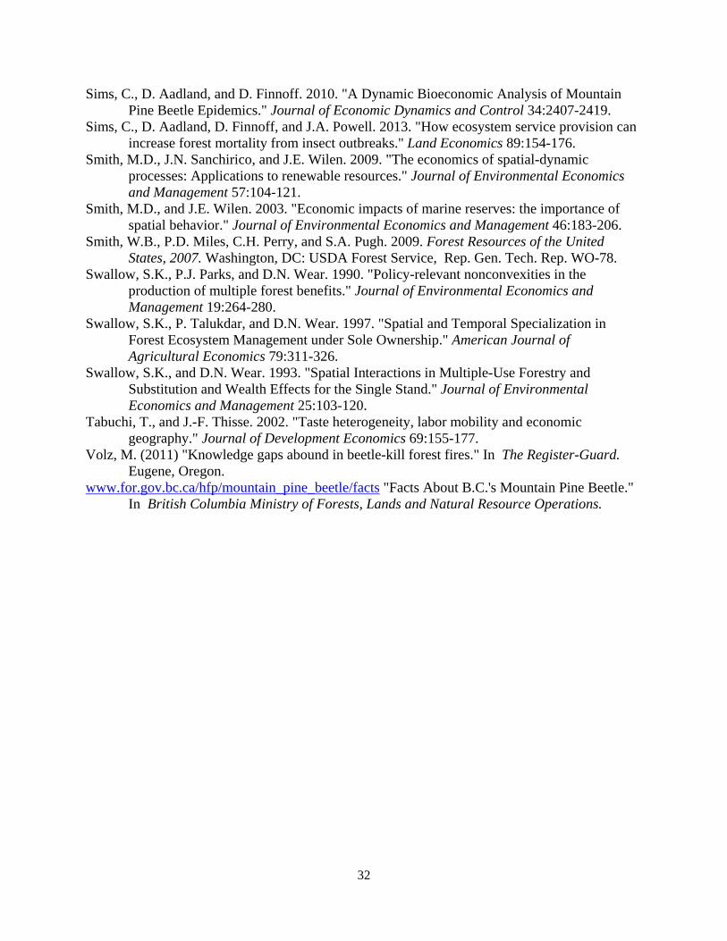
MPB and boundary forests (types 4 and 6) repelling MPB (figure 3 presents the local harvesting

case). Third, harvests and tree stocks vary significantly based on forest type. Position on the

grid creates differential MPB risk even for forests that are otherwise identical. This differential

MPB risk leads to a complex spatial configuration of tree stocks, MPB and harvests (figure 3).

Types 4 and 6 (boundary forests) have the densest forests, the most harvesting and the lowest

MPB stocks. Types 2 and 3 (intermediate forests) have the sparsest forests, the least harvesting

and the highest MPB stocks. As a result, stakeholders in type 4 and 6 forests receive the highest

utility while type 2 and 3 stakeholders receive the lowest utility. Fourth, stocks, harvests and

                                                            9 For the vast majority of calibrations and for a wide range of starting values, the system contains a unique interior steady state and satisfies the saddle-path stability condition. See the sensitivity analysis in the Appendix for the cases where an interior steady state could not be found.

19  

utility levels are similar for local and central harvesting. This occurs because the migration

externality (which results in over-harvesting of adult trees as local managers encourage

migration off their forest) largely offsets the reproduction externality (which results in under-

harvesting as local managers ignore the costs to neighboring forests of a new MPB cohort). As a

result, there is a reduced need for central management to intervene and dictate harvesting quotas

on local forests. In the appendix, we investigate the sensitivity of this result to variation in the

fundamental parameters.

3.4.2 Transition Dynamics after a MPB Outbreak

Figures 4 and 5 contrast the impacts of optimal and no harvesting on the spatiotemporal

dynamics of beetles and adult trees after a MPB outbreak. As MPB are native and endemic,

there are no long-run equilibrium effects of the outbreak. There are however significantly

different transition effects depending on the management regime. Figure 6 displays optimal

local and central harvest paths to highlight the differences in management responses after the

outbreak. All three figures show the dynamics over 15 years following the initial outbreak

across the entire 6 6 landscape grid. Note that the vertical scale on the figures is not fixed in

order to emphasize the pattern of the impulse response.

The MPB populations are displayed in figure 4 with thick, solid and dashed lines

representing no, local and central harvesting (the solid and dashed lines are sometimes close

together and difficult to distinguish). The intercepts on the vertical axis mark the endemic

steady-state levels of MPB on each local forest. At 1 an outbreak occurs in cell (1,1),

elevating the MPB population to approximately 13,000 MPB per acre. The new MPB attack

adult pine trees in cell (1,1), laying eggs under the bark, killing the trees, and producing the next

20  

generation of MPB. In period 2, the new MPB emerge from trees and begin to search for

new hosts. The initial outbreak kills nearly 10% of the adult trees in cell (1,1) causing many of

the MPB to disperse to neighboring cells. They then attack trees in the neighboring cells and

start the reproduction process over again. The migration and reproduction process continues

over space and time until the outbreak has dispersed over the entire grid and dissipated through

time. Figure 5 shows that adult tree densities across the grid are lower after the outbreak, but

they gradually regenerate as younger trees mature to the adult category. MPB also spread to

neighboring cells at a greater rate under optimal harvesting than under no harvesting. We

discuss this effect further in the next section.

Figure 6 displays the optimal local and central harvesting strategies. Steady-state, initial

harvest levels are similar for centralized planning (dashed lines) and local planning (solid lines).

After the outbreak, harvest levels immediately increase across the grid. In cell (1,1), the local

forest manager responds immediately to the local outbreak by harvesting additional adult trees

because the expected future value of a tree declines. In the neighboring forests, cells (1,2), (2,2)

& (2,1), managers also increase their harvesting in 1, as they anticipate the effects of the

outbreak spreading to their forest in 2. Immediate harvesting has the benefit of providing

additional timber products but also reduces the likelihood that MPB from the epidemic disperse

to your local forest. The increased harvesting on neighboring cells causes additional beetles to

leave these cells in 2. Most of these beetles will disperse to cells (1,3), (2,3), (3,3), (3,2),

and (3,1) in 2 since there are fewer susceptible host trees in cell (1,1) due to the outbreak.

Anticipating this influx of MPB in 2, managers two cells away from the outbreak

immediately increase harvest levels in 1. Likewise, managers three cells away from the

outbreak immediately increase harvest levels in 1 in response to the increase in harvests in

21  

all northwest cells. This highlights how a biological shock to local timber markets (the outbreak)

is transferred across space due to the physical movement of the MPB and due to the expectations

of local forest managers. Even though the effect of the outbreak will not reach other forests for

at least two periods, the additional harvesting on neighboring cells in 1 creates a ripple effect

that encourages all managers to immediately increase harvest levels. As the stock of adult trees

decline, harvest levels gradually drop and fall below steady-state levels due to the increasing

marginal non-timber value of each adult tree. With central planning, there is a similar but

smoother pattern, with the initial increase in harvesting being less steep and the decline more

gradual.

3.4.3 Contrasting the Degree of Spread: Optimal versus No Harvesting

A comparison of the transition paths over management regimes reveals a potential tradeoff

caused by a MPB outbreak. Outbreaks under no harvesting are severe with high aggregate MPB

abundances and high degrees of MPB induced tree mortality, but lower rates of dispersal across

the landscape. In contrast, outbreaks with optimal harvesting see a reduction in severity, yet the

MPB disperse across the landscape at a higher rate. Optimal harvesting allows humans to

anticipate the MPB-induced mortality, harvest the trees before they are attacked, capture the

value of the trees from the market, and moderate the severity of the outbreak.10 However, there

is an ecological feedback response. MPB disperse quicker in their search for prey, which in turn

moderates the incentive to harvest. The combined outcome sees a less severe outbreak but more

                                                            10 See Holmes (1991) and Prestemon and Holmes (2004) for more information on the impact of beetle outbreaks on timber markets.

22  

spread over the landscape. These interdependencies are not present in aspatial models (or spatial

models of a single species) and provide a clear contribution of this work.

The consequences of the tradeoff also vary at different points in the landscape. To illustrate,

consider a MPB outbreak that occurs at 1 in cell (1,1) and gradually spreads across the grid.

To measure the degree of MPB spread, we calculate the deviation of MPB from their endemic,

steady-state level, , , at a point in time after the outbreak. This measure captures pure MPB

migration but also includes other factors that influence MPB population such as reproductive

efficiency. Since there are more trees and fewer beetles on the borders, we contrast MPB spread

in two directions – along the top border , , , , , , , , , and down the

diagonal , , , , , , , , , .11 Figure 7 graphs the difference in , under local

and no harvesting. The graph captures the influence of harvesting on MPB spread with positive

values indicating that harvesting leads to more MPB spread.12 The figure highlights the tradeoff

between the severity and extent of MPB epidemics: harvesting effectively limits the severity of

MPB outbreaks but encourages MPB migration and increases the spread rate for MPB

epidemics. The nature of this tradeoff will differ over space given the differences in spread

along the border and diagonal.

4. Computational Efficiency and Numerical Approximations

Here we discuss the computational efficiency of our algorithm and present a more in-depth

analysis of our two approximations: (1) linearization of the harvest rules and (2) truncation of

                                                            11 Due to the symmetry of the landscape grid, horizontal and vertical spread originating from the (1,1) cell will be equal. 12 The graphs are qualitatively similar for the comparison between central management and no harvesting. Results are available upon request.

23  

the endogenous migration effects. It is not possible to calculate the exact magnitude of the total

approximation error as this would require solving the full nonlinear spatial optimization problem.

We were unable to solve this problem, even on a grid as small as 2 × 2. We instead investigate

the magnitude of each approximation error separately and report the results in subsections 4.2

and 4.3. Our conclusion is that both approximation errors are negligible, and the method will

provide a close fit to the true optimal management rule.

4.1 Computational Efficiency

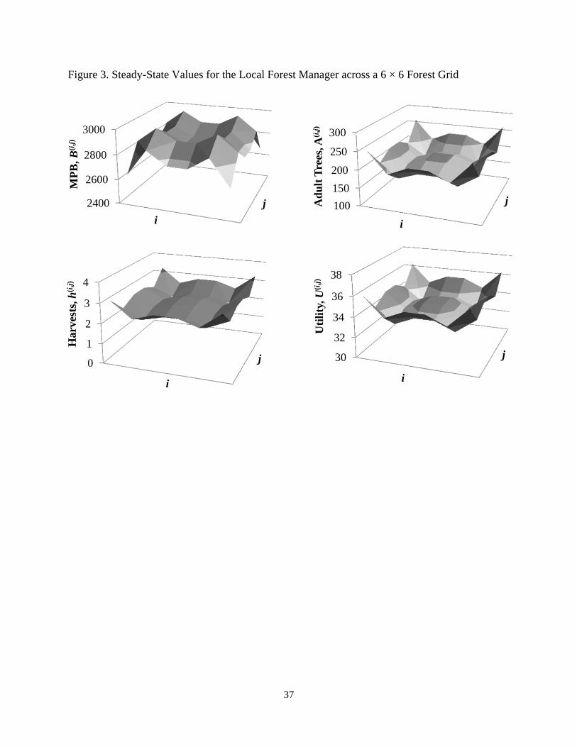
In Figure 8, we graph the computational time for our algorithm against various (square) grid

sizes. A quadratic trend line fits the data points perfectly indicating that the computational time,

, can be expressed as ∈ , where is the number of cells in the grid. Our

linearization is capable of solving for the optimal local harvest rule on a grid as large as 20 20

in only 5300 CPU seconds. By contrast, we were unable to solve the non-linear local planner

problem for even a 6 6 grid or the non-linear central planner problem for even a 2 2 grid.

4.2 Linearization of the Harvest Rules

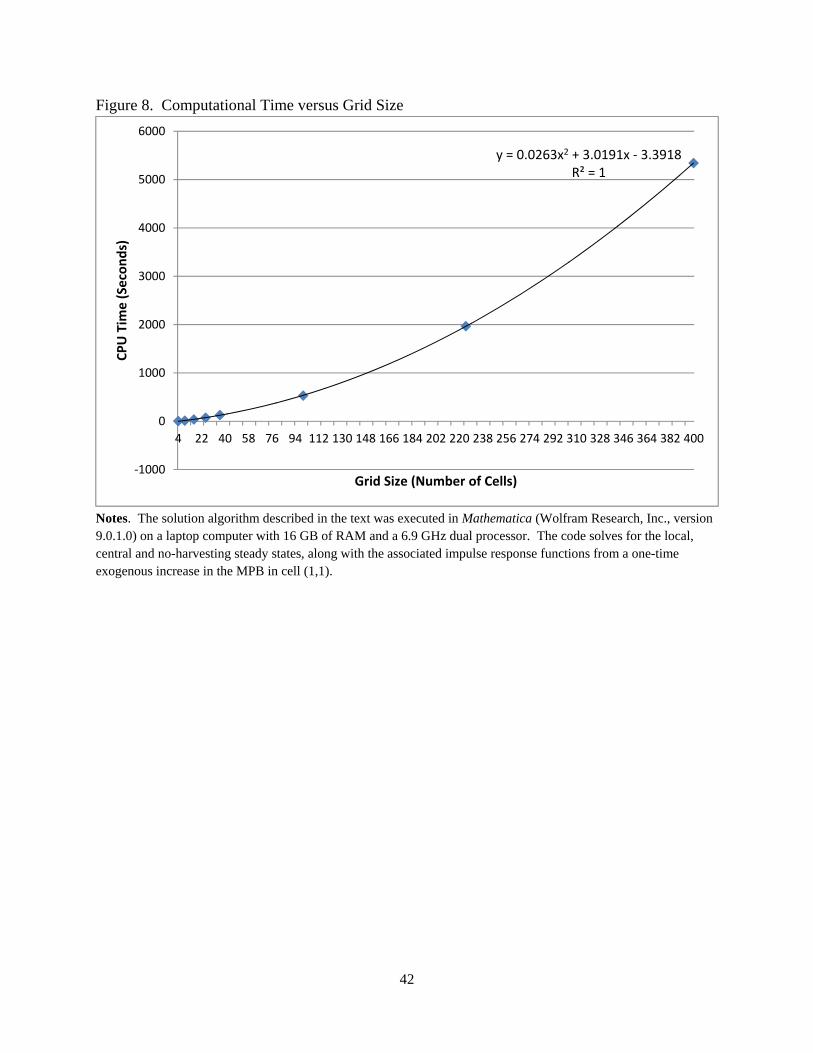
To determine how well the linearized rule approximates the nonlinear harvest rule, we

calculate optimal decentralized nonlinear harvests paths on a smaller 4×4 grid using the PATH

solver in GAMS (GAMS Development Corporation, 2006). We then applied the linearized

harvest rule to the same 4×4 grid. The approximation error increases with the size of the initial

MPB shock and tends to decrease as time passes and both harvest rules return to steady state.

Spatially, the approximation error is also largest in the cell where the shock takes place, cell (1,1)

in our simulations (see Figure 9). The linear and nonlinear harvest rules produced similar

24  

harvest paths with the linear harvest rule successfully replicating the cyclical dynamics present in

the complete nonlinear model. The linear and nonlinear harvest rules differ by no more than

10% when the shock takes place. This difference quickly dissipates to less than 5% in the next

period. As the linear harvest rule is implemented in conjunction with the nonlinear biological

system, this translates into an even smaller difference in stocks. For instance, adult tree stocks

differ by less than 0.2%.

We also calculate optimal linear and nonlinear harvests paths on 1×1, 2×2, and 3×3 grids

and find that a larger grid size does not necessarily imply a larger linear approximation error

(figures are available upon request). Initially the maximum percent deviation between linear and

nonlinear harvest paths grows as one increases spatial scale from a 1×1 to 2×2 to 3×3 grid.

However, the maximum percent deviation between linear and nonlinear harvest paths begins to

decline when spatial scale increases further to the 4×4 grid. While a larger grid implies more

approximated harvest decisions, it also allows the largest approximation error in cell (1,1) to be

dissipated as MPB spread to neighboring cells. This indicates that approximation error in our

results associated with a 6×6 grid is likely to be modest. In sum, we feel our methodology is a

significant step forward because it is capable of offering reasonable management prescriptions

for decentralized spatial optimization problems that were otherwise thought to be intractable.

4.3 Truncation of the Endogenous Migration Effects

Here we investigate the magnitude of multi-cell endogenous migration effects. Recall that

our solution procedure allows the forest manager to consider all future exogenous migration

25  

effects but restricts the manager to only consider endogenous migration effects that work through

neighboring forests. Due to this truncation, the terms

, / , (15)

for 3 are missing from equation (11). These terms in (15) capture how harvesting decisions

in period (which directly affect , ) impact MPB risk three periods or more into the future

through multi-cell migration. Direct calculation of these terms is extremely complicated and

likely to be infeasible. Although we have derived analytic expressions for the 3 effect

(the 1 and 2 effects are shown in the Appendix), programming the optimal harvesting

rule with these higher-order multi-cell migration effects is impractical. As a second-best

approach, we use other information to argue that these endogenous multi-cell migration terms are

unlikely to have a significant impact on harvesting decisions and the associated state variables.

First, the endogenous migration effects in (15) are likely to dissipate over time and space as

grows. If not, the total impact of these effects would grow without bound as planners look into

the indefinite future. Although we are unable to calculate the full set of endogenous migration

effects, we are able to calculate (15) at the endemic steady state for = 1, 2, and 3. For our

calibration, these impacts decrease as grows. For a 6 6 grid, the 2 and 3 endogenous

migration terms are approximately 50% and 25% of the 1 term, respectively. This suggests

that truncating the endogenous migration terms past the neighbor effect is likely to have a

negligible impact on the optimal harvest rules.

Second, the relative impact of the endogenous migration terms in (15) appears to be fairly

stable off steady state. As stated in the paragraph directly above, the steady-state endogenous

migration terms decline as increases from 1 to 2 to 3. Because these terms are

26  

getting progressively smaller, truncation of the future endogenous migration terms is unlikely to

have a substantial impact on optimal harvesting levels at steady state. To get an idea of whether

this also holds off steady state, we calculated local harvesting levels with and without the 2

endogenous migration term after a MPB outbreak. Figure 10 shows that optimal local harvesting

levels with and without the 2 endogenous migration terms share a similar pattern with

slightly more harvesting when the 2 endogenous migration terms are included. This suggests

that truncation of future endogenous migration effects past 2 is likely to have a negligible

impact on optimal timber harvests, both at steady state and during an outbreak.

Third, and finally, the complexity of the endogenous migration partial derivatives grow so

fast that we were unable to analytically calculate these terms beyond the 3 effect. It seems

reasonable that local planners may have similar difficulties in calculating these effects and

rationally choose to ignore the impact that their harvesting decision will have on their own future

welfare through this type of multi-cell migration. Similar arguments have been made in the

literature on spatial discounting on the basis that external effects of economic activity are

spatially diffused at positive rates (Perrings and Hannon, 2001).

Truncation of the higher-order endogenous migration terms appears to provide reasonable

optimal harvest levels for our application where half the MPB disperse to other cells in steady

state. However, it is likely that the approximation will be less accurate in applications where the

dispersal rate is very high and the majority of the migrating state variable leave the cell each

period. In these applications, the use of our approximation method requires caution.

In sum, we feel the evidence presented above suggests that our method will provide reasonable

solutions to the optimal management problems in a wide range of spatial bioeconomic systems

with continuous controls and migrating states.

27  

5. Conclusions

This paper builds on and extends an emerging spatial literature in environmental and natural

resource economics. Borrowing from solution techniques in macroeconomics, we solve for

explicit local harvesting rules that incorporate current and future spatial risks from insect

outbreaks. The harvest rules are a function of the current tree and insect stocks from every cell

on the grid. While our application focuses on insect outbreaks, the method is sufficiently general

to be applicable to a wide range of spatially and temporally dynamic economic systems.

Methodologically, the most important feature of the optimal harvest rules is that they only

depend on current stocks. Therefore, rather than needing to collectively solve the entire set of

first-order conditions and biological equations, the system collapses to a recursive set of simpler

two-period tasks. For problems of local optimal control, this procedure allows for a much larger

grid even in the presence of spatial interdependencies. While the procedure requires two

approximations, these had a negligible impact in the spatial bioeconomic system we considered.

For problems of central optimal control that rely on gradient-based search algorithms

(Rassweiler, et al., 2012), computational cost can be reduced by using our approximation method

to provide starting values for these algorithms.

In terms of natural resource policy, we highlight two features of the bioeconomic model.

First, harvesting increases the rate of pest spread and has important spatial consequences. In our

application, this occurs because timber harvesting results in less dense stands of timber and

therefore MPB migrate to neighboring forests at a greater rate. Harvesting therefore dampens

outbreaks but causes them to spread faster over the landscape. Second, we find that centralized

28  

harvesting strategies produce harvests, forest densities, and welfare levels that are similar to

those under local planning. This occurs because the migration and reproduction externalities

associated with local planning work in opposing directions. The migration externality

encourages local over-harvesting so more MPB migrate to neighboring forests, while the

reproduction externality encourages under-harvesting as local planners fail to recognize that

dense forests lead to more MPB and elevated MPB risk on neighboring forests. The sensitivity

analysis shows that although these two externalities will always have opposite sign, they are not

always of equal magnitude. This implies that the role for central management will vary across

areas with differing rates of resource growth and pest susceptibility.

Many challenges remain in the spatially optimized management of bioeconomic systems.

Much of the economic literature is built on a grid-based representation of the environment where

management takes place on a cell and state variables migrate between cells. This implies that

local management and dispersal take place on the same spatial scale which may be restrictive in

many settings (Borgström, et al., 2006, Cash, et al., 2006, Cumming, et al., 2006). Increased use

of dispersal kernels in bioeconomic modeling allows for a continuous representation of migration

that could address this scale mismatch. Also, dispersal in many spatial bioeconomic systems

may not be solely governed by density dependence. Human-mediated dispersal vectors such as

trucking and individual travel could be incorporated with a more general dispersal equation.

Similar techniques have been used in gravity models of invasive species spread (Bossenbroek, et

al., 2001, Buchan and Padilla, 1999, Leung, et al., 2006). These issues are reserved for future

research.

29  

References

Abbott, B., B. Stennes, and G.C. van Kooten. 2009. "Mountain pine beetle, global markets, and the British Columbia forest economy." Canadian Journal of Forest Research 39:1313-1321.

Albers, H.J. 1996. "Modeling Ecological Constraints on Tropical Forest Management: Spatial Interdependence, Irreversibility, and Uncertainty." Journal of Environmental Economics and Management 30:73-94.

Albers, H.J., C. Fischer, and J.N. Sanchirico. 2010. "Invasive species management in a spatially heterogeneous world: Effects of uniform policies." Resource and Energy Economics 32:483-499.

Azariadis, C. 1993. Intertemporal Macroeconomics. Cambridge, MA: Blackwell Publishers. Bentz, B.J. 2006. "Mountain pine beetle population sampling: inferences from Lindgren

pheromone traps and tree emergence cages." Canadian Journal of Forest Research 36:351-360.

Berryman, A.A., B. Dennis, K.F. Raffa, and N.C. Stenseth. 1985. "Evolution of optimal group attack, with particular reference to bark beetles (Coleoptera: Scolytidae)." Ecology 66:898-903.

Bhat, M.G., and R.G. Huffaker. 2007. "Management of a transboundary wildlife population: A self-enforcing cooperative agreement with renegotiation and variable transfer payments." Journal of Environmental Economics and Management 53:54-67.

Bhat, M.G., R.G. Huffaker, and S.M. Lenhart. 1996. "Controlling transboundary wildlife damage: modeling under alternative management scenarios." Ecological Modeling 92:215-224.

Blanchard, O.J., and C.M. Kahn. 1980. "The Solution of Linear Difference Models under Rational Expectations." Econometrica 48:1305-1311.

Borgström, S.T., T. Elmqvist, P. Angelstam, and C. Alfsen-Norodom. 2006. "Scale mismatches in management of urban landscapes." Ecology and Society 11:16.

Bossenbroek, J.M., C.E. Kraft, and J.C. Nekola. 2001. "Prediction of long-distance dispersal using gravity models: zebra mussel invasion of inland lakes." Ecological Applications 11:1778-1788.

Brock, W., and A. Xepapadeas. 2008. "Diffusion-induced instability and pattern formation in infinite horizon recursive optimal control." Journal of Economic Dynamics and Control 32:2745-2787.

---. 2010. "Pattern formation, spatial externalities and regulation in coupled economic-ecological systems." Journal of Environmental Economics and Management 59:149-164.

Brown, G., and J. Roughgarden. 1997. "A metapopulation model with private property and a common pool." Ecological Economics 22:65-71.

Buchan, L.A., and D.K. Padilla. 1999. "Estimating the probability of long-distance overland dispersal of invading aquatic species." Ecological Applications 9:254-265.

Bulte, E.H., and G.C. van Kooten. 1999. "Metapopulation dynamics and stochastic bioeconomic modeling." Ecological Economics 30:293-299.

Cash, D.W., W.N. Adger, F. Berkes, P. Garden, L. Lebel, P. Olsson, L. Pritchard, and O. Young. 2006. "Scale and cross-scale dynamics: governance and information in a multilevel world." Ecology and Society 11:8.

30  

Clarida, R., J. Galí, and M. Gertler. 2000. "Monetary Policy Rules and Macroeconomic Stability: Evidence and Some Theory." Quarterly Journal of Economics 115:147-180.

Cole, W.E. 1983. Interaction between Mountain Pine Beetle and Dynamics of Lodgepole Pine Stands. United States Department of Agriculture, Forest Service Res. Note INT-170, Rep. Res. Note INT-170.

Cole, W.E., and M.D. McGregor. 1983. Estimating the rate and amount of tree loss from mountain pine beetle infestations: US Department of Agriculture, Forest Service, Intermountain Forest and Range Experiment Station.

Cooley, T.F., and E.C. Prescott (1995) "Economic Growth and Business Cycles." In T.F. Cooley ed. Frontiers of Business Cycle Research. Princeton, NJ, Princeton University Press.

Costello, C., and S. Polasky. 2008. "Optimal harvesting of stochastic spatial resources." Journal of Environmental Economics and Management 56:1-18.

Cumming, G.S., D.H. Cumming, and C.L. Redman. 2006. "Scale mismatches in social-ecological systems: causes, consequences, and solutions." Ecology and Society 11:14.

Dockner, E.J., S. Jorgensen, N. Van Long, and G. Sorger. 2012. Differential games in economics and management science: Cambridge University Press.

Epanchin-Niell, R.S., and J.E. Wilen. 2012. "Optimal spatial control of biological invasions." Journal of Environmental Economics and Management 63:260-270.

Farmer, R.E.A. 2002. Macroeconomics of Self-fulfilling Prophecies. 2nd ed. ed. Cambridge, MA: The MIT Press.

Fredriksson, P.G., and D.L. Millimet. 2002. "Strategic interaction and the determination of environmental policy across US states." Journal of Urban Economics 51:101-122.

Fujita, M., P. Krugman, and A.J. Venables. 1999. The Spatial Economy: Cities, Regions, and International Trade. Cambridge, MA: MIT Press.

GAMS Development Corporation. 2006. GAMS Release 22.2 Version 145, Washington, D.C. Heavilin, J., and J. Powell. 2008. "A novel method of fitting spatio-temporal models to data, with

applications to the dynamics of mountain pine beetles." Natural Resource Modeling 21:489-524.

Hof, J.G., M. Bevers, L.A. Joyce, and B. Kent. 1994. "An Integer Programming Approach for Spatially and Temporally Optimizing Wildlife Populations." Forest Science 40:177-191.

Holmes, T.P. 1991. "Price and welfare effects of catastrophic forest damage from southern pine beetle epidemics." Forest Science 37:500-516.

Horan, R.D., C.A. Wolf, E.P. Fenichel, and K.H. Matthews Jr. 2005. "Spatial Management of Wildlife Disease." Review of Agricultural Economics 27:483-490.

Kaffine, D.T., and C. Costello. 2011. "Unitization of Spatially Connected Renewable Resources." The B.E. Journal of Economics Analysis and Policy 11:Article 15.

Koch, P. 1996. Lodgepole Pine in North America: Forest Products Society. Konoshima, M., C.A. Montgomery, H.J. Albers, and J.L. Arthur. 2008. "Spatial-endogenous fire

risk and efficient fuel management and timber harvest." Land Economics 84:449-468. Krugman, P. 1991. Geography and Trade. Cambridge, MA: MIT Press. Kuang, Y., and Y. Takeuchi. 1994. "Predator-prey dynamics in models of prey dispersal in two-

patch environments." Mathematical Biosciences 120:77-98. Kurz, W.A., C.C. Dymond, G. Stinson, G.J. Rampley, E.T. Neilson, A. Carroll, T. Ebata, and L.

Safranyik. 2008. "Mountain pine beetle and forest carbon feedback to climate change." Nature 452:987-990.

31  

Leung, B., J.M. Bossenbroek, and D.M. Lodge. 2006. "Boats, pathways, and aquatic biological invasions: estimating dispersal potential with gravity models." Biological Invasions 8:241-254.

Logan, J.A., J. Regniere, and J.A. Powell. 2003. "Assessing the impacts of global warming on forest pest dynamics." Frontiers in Ecology and the Environment 1:130-137.

Lotan, J.E., and W.B. Critchfield (1990) "Pinus contorta Dougl. ex Loud." In R.M. Burns, and B.H. Honkala eds. Silvics of North America Vol. 1 confiers. Washington, D.C., US Department of Agriculture, pp. 302-315.

Millennium Ecosystem Assessment, 2005 "Ecosystems and Human Well-Being: Synthesis." Island Press, Washington, DC.

Patriquin, M.N., A.M. Wellstead, and W.A. White. 2007. "Beetles, trees, and people: Regional economic impact sensitivity and policy considerations related to the mountain pine beetle infestation in British Columbia, Canada." Forest Policy and Economics 9:938-946.

Perrings, C., and B. Hannon. 2001. "An introduction to spatial discounting." Journal of Regional Science 41:23-38.

Pfeiffer, D., T. Robinson, M. Stevenson, K.B. Stevens, D.J. Rogers, and A.C.A. Clements. 2008. Spatial analysis in epidemiology. New York: Oxford University Press.

Phillips, B.R., J.A. Breck, and T.J. Nickel. 2007. Title."Unpublished, Institution|. Prestemon, J., P., and T. Holmes, P. 2004. "Market Dynamics and Optimal Timber Salvage After

a Natural Catastrophe." Forest Science 50:495-511. Rassweiler, A., C. Costello, and D.A. Siegel. 2012. "Marine protected areas and the value of

spatially optimized fishery management." Proceedings of the National Academy of Sciences 109:11884-11889.

Rosie, J.P. 1990. "Multicriteria Nonlinear Programming for Optimal Spatial Allocation of Stands." Forest Science 36:487-501.

Row, C., H.F. Kaiser, and J. Sessions. 1981. "Discount rate for long-term Forest Service investments." Journal of Forestry 79:367-369.

Safranyik, L., and A. Carroll (2006) "The biology and epidemiology of the mountain pine beetle in lodgepole pine forests." In L. Safranyik, and B. Wilson eds. The Mountain Pine Beetle: A Synthesis of Its Biology, Management and Impacts on Lodgepole Pine. Victoria, British Columbia, Canadian Forest Service, Pacific Forestry Centre, Natural Resources Canada, pp. 3-66.

Safranyik, L., D.A. Linton, R. Silversides, and L. McMullen. 1992. "Dispersal of released mountain pine beetles under the canopy of a mature lodgepole pine stand." Journal of Applied Entomology 113:441-450.

Safranyik, L., D.M. Shrimpton, and H. Whitney. 1974. Management of Lodgepole Pine to Reduce Losses from the Mountain Pine Beetle. Canadian Forest Service, Pacific Forest Research Station, Forest Technical Report 1:24, Rep. Forest Technical Report 1:24.

Samman, S., and J. Logan. 2000. Assessment and response to bark beetle outbreaks in the Rocky Mountain area. USDA Forest Service, Rep. RMRS-GTR-62.

Sanchirico, J., J.E. Wilen, and C. Coleman. 2010. "Optimal Rebuilding of a Metapopulation." American Journal of Agricultural Economics 92:1087-1102.

Sanchirico, J.N., and J.E. Wilen. 1999. "Bioeconomics of Spatial Exploitation in a Patchy Environment." Journal of Environmental Economics and Management 37:129-150.

---. 2005. "Optimal spatial management of renewable resources: matching policy scope to ecosystem scale." Journal of Environmental Economics and Management 50:23-46.

32  

Sims, C., D. Aadland, and D. Finnoff. 2010. "A Dynamic Bioeconomic Analysis of Mountain Pine Beetle Epidemics." Journal of Economic Dynamics and Control 34:2407-2419.

Sims, C., D. Aadland, D. Finnoff, and J.A. Powell. 2013. "How ecosystem service provision can increase forest mortality from insect outbreaks." Land Economics 89:154-176.

Smith, M.D., J.N. Sanchirico, and J.E. Wilen. 2009. "The economics of spatial-dynamic processes: Applications to renewable resources." Journal of Environmental Economics and Management 57:104-121.

Smith, M.D., and J.E. Wilen. 2003. "Economic impacts of marine reserves: the importance of spatial behavior." Journal of Environmental Economics and Management 46:183-206.

Smith, W.B., P.D. Miles, C.H. Perry, and S.A. Pugh. 2009. Forest Resources of the United States, 2007. Washington, DC: USDA Forest Service, Rep. Gen. Tech. Rep. WO-78.

Swallow, S.K., P.J. Parks, and D.N. Wear. 1990. "Policy-relevant nonconvexities in the production of multiple forest benefits." Journal of Environmental Economics and Management 19:264-280.

Swallow, S.K., P. Talukdar, and D.N. Wear. 1997. "Spatial and Temporal Specialization in Forest Ecosystem Management under Sole Ownership." American Journal of Agricultural Economics 79:311-326.

Swallow, S.K., and D.N. Wear. 1993. "Spatial Interactions in Multiple-Use Forestry and Substitution and Wealth Effects for the Single Stand." Journal of Environmental Economics and Management 25:103-120.

Tabuchi, T., and J.-F. Thisse. 2002. "Taste heterogeneity, labor mobility and economic geography." Journal of Development Economics 69:155-177.

Volz, M. (2011) "Knowledge gaps abound in beetle-kill forest fires." In The Register-Guard. Eugene, Oregon.

www.for.gov.bc.ca/hfp/mountain_pine_beetle/facts "Facts About B.C.'s Mountain Pine Beetle." In British Columbia Ministry of Forests, Lands and Natural Resource Operations.

   

33  

Table 1. Model parameters

Parameter Definition Value

Rate of germination of seeds in seed base 0.001

Rate of maturation of young trees 0.0019

Rate of viable seed production in young trees 0.0018

Rate of viable seed production in adult trees 0.0018

Number of MPB/acre required for a 50% chance of MPB-induced mortality in adult trees in 1990 63,800

Average MPB offspring per infested tree 4,500

Rate of natural adult tree mortality 0.02

Rate of decrease in beetle reproduction with increases in beetle-induced mortality in adult trees

0.5

Discount factor 0.96

 Relative preference for non-timber versus timber benefits

6.23

  Own-cell dispersal parameter varies by type

  Own-cell dispersal parameter 10

Notes. The preference parameter is selected so average steady-state harvests for the local forest manager equal 2.5. The own-cell dispersal parameter varies by steady-state type and is selected so , → , 0.5.

34  

Table 2. Steady-State Values for No, Local, and Central Harvesting

Variable (per acre)

Type

1 2 3 4 5 6

No

Har

vest

ing

MPB, , 7657.21 7657.21 7657.21 7657.21 7657.21 7657.21

Adult Trees, , 203.02 161.93 183.04 224.25 198.62 258.38

Harvests, , 0 0 0 0 0 0

Loc

al H

arve

stin

g

MPB, , 2771.68 2930.46 2847.68 2710.46 2813.00 2605.37

Adult Trees, , 201.09 163.97 182.78 221.98 198.68 255.27

Harvests, , 2.48 1.98 2.23 2.75 2.44 3.20

Utility, , 34.03 32.53 33.33 34.75 33.94 35.77

Cen

tral

Har

vest

ing

MPB, , 2927.80 3133.46 3026.12 2850.02 2983.64 2714.22

Adult Trees, , 201.32 164.98 183.35 222.04 199.26 255.00

Harvests, , 2.44 1.95 2.19 2.71 2.40 3.16

Utility, , 34.02 32.55 33.33 34.73 33.94 35.75

Notes. Steady-state values use the parameters in Table 1. See Figure 1 for the grid position of each type. Local and central optimal harvesting are calculated using equations (11) and (14).

35  

Figure 1. Stylized Representation of the Forest Landscape and Beetle Dispersal

Type 6

(1,1)

Type 5

(1,2)

Type 4

(1,3)

Type 4

(1,4)

Type 5

(1,5)

Type 6

(1,6)

Type 5

(2,1)

Type 3

(2,3)

Type 3

(2,4)

Type 2

(2,5)

Type 5

(2,6)

Type 4

(3,1)

Type 3

(3,2)

Type 1

(3,3)

Type 1

(3,4)

Type 3

(3,5)

Type 4

(3,6)

Type 4

(4,1)

Type 3

(4,2)

Type 1

(4,3)

Type 1

(4,4)

Type 3

(4,5)

Type 4

(4,6)

Type 5

(5,1)

Type 2

(5,2)

Type 3

(5,3)

Type 3

(5,4)

Type 2

(5,5)

Type 5

(5,6)

Type 6

(6,1)

Type 5

(6,2)

Type 4

(6,3)

Type 4

(6,4)

Type 5

(6,5)

Type 6

(6,6)

Notes. The green shaded area represents the forest landscape while the brown shaded area is the non-forested perimeter. There are six types of cells based on symmetric grid positions. Each cell contains an , index representing row and column . The figure in cell (2,2) represents beetle dispersal to neighboring cells based on a queen contiguity pattern.

Non‐Forested Region 

36  

Figure 2. Dispersal Function for MPB Remaining on Own Cell (Type 1)

Notes. The own-dispersal weight is , → , 1 exp c A , , where c 0.0047 and c 10.

0.0

0.2

0.4

0.6

0.8

1.0

10 30 50 70 90 110 130 150 170 190 210 230 250 270 290 310 330

Fraction of MPB Rem

aining on Own Cell

Adult Stock (A)

37  

Figure 3. Steady-State Values for the Local Forest Manager across a 6 × 6 Forest Grid

2400

2600

2800

3000

j

MP

B, B

(i,j)

i100

150

200

250

300

jAd

ult

Tre

es, A

(i,j)

i

0

1

2

3

4

j

Har

vest

s, h

(i,j)

i

30

32

34

36

38

j

Uti

lity

, U(i

,j)

i

38  

Figure 4. Landscape Mountain Pine Beetle (MPB) Dispersal after Local Outbreak

Notes. The thick solid line represents MPB dynamics under no harvesting. The solid (dashed) lines represent MPB dynamics under optimal local (central) planning. The vertical axis measures number of MPB per acre on each local forest; the horizontal axis measures time in years. A MPB outbreak occurs in cell (1,1) at time 1. The initial outbreak is ten times the steady-state MPB population in cell (1,1). The initial outbreak is restricted to be equal under the three cases.

0 2 4 6 8 10 12 140

2000400060008000

1000012000

Cell 1, 1

0 2 4 6 8 10 12 140

2000400060008000

Cell 1, 2

0 2 4 6 8 10 12 140

2000400060008000

Cell 1, 3

0 2 4 6 8 10 12 140

2000400060008000

Cell 1, 4

0 2 4 6 8 10 12 140

2000400060008000

Cell 1, 5

0 2 4 6 8 10 12 140

2000400060008000

Cell 1, 6

0 2 4 6 8 10 12 140

2000400060008000

Cell 2, 1

0 2 4 6 8 10 12 140

2000400060008000

Cell 2, 2

0 2 4 6 8 10 12 140

2000400060008000

Cell 2, 3

0 2 4 6 8 10 12 140

2000400060008000

Cell 2, 4

0 2 4 6 8 10 12 140

2000400060008000

Cell 2, 5

0 2 4 6 8 10 12 140

2000400060008000

Cell 2, 6

0 2 4 6 8 10 12 140

2000400060008000

Cell 3, 1

0 2 4 6 8 10 12 140

2000400060008000

Cell 3, 2

0 2 4 6 8 10 12 140

2000400060008000

Cell 3, 3

0 2 4 6 8 10 12 140

2000400060008000

Cell 3, 4

0 2 4 6 8 10 12 140

2000400060008000

Cell 3, 5

0 2 4 6 8 10 12 140

2000400060008000

Cell 3, 6

0 2 4 6 8 10 12 140

2000400060008000

Cell 4, 1

0 2 4 6 8 10 12 140

2000400060008000

Cell 4, 2

0 2 4 6 8 10 12 140

2000400060008000

Cell 4, 3

0 2 4 6 8 10 12 140

2000400060008000

Cell 4, 4

0 2 4 6 8 10 12 140

2000400060008000

Cell 4, 5

0 2 4 6 8 10 12 140

200040006000

Cell 4, 6

0 2 4 6 8 10 12 140

2000400060008000

Cell 5, 1

0 2 4 6 8 10 12 140

2000400060008000

Cell 5, 2

0 2 4 6 8 10 12 140

2000400060008000

Cell 5, 3

0 2 4 6 8 10 12 140

2000400060008000

Cell 5, 4

0 2 4 6 8 10 12 140

200040006000

Cell 5, 5

0 2 4 6 8 10 12 140

200040006000

Cell 5, 6

0 2 4 6 8 10 12 140

2000400060008000

Cell 6, 1

0 2 4 6 8 10 12 140

2000400060008000

Cell 6, 2

0 2 4 6 8 10 12 140

2000400060008000

Cell 6, 3

0 2 4 6 8 10 12 140

200040006000

Cell 6, 4

0 2 4 6 8 10 12 140

200040006000

Cell 6, 5

0 2 4 6 8 10 12 140

200040006000

Cell 6, 6

39  

Figure 5. Adult Trees Stock after Local MPB Outbreak

Notes. The thick solid line represents adult tree stocks under no harvesting. The solid (dashed) lines represent adult tree stocks under optimal local (central) planning. The vertical axis measures the number of adult trees per acre on each local forest. The horizontal axis measures time in years. A MPB outbreak occurs in cell (1,1) at time 1.

0 2 4 6 8 10 12 14235240245250255

Cell 1, 1

2 4 6 8 10 12 14188190192194196198

Cell 1, 2

0 2 4 6 8 10 12 14

216218220222224

Cell 1, 3

0 2 4 6 8 10 12 14218219220221222223224

Cell 1, 4

0 2 4 6 8 10 12 14

197.5198.0198.5199.0

Cell 1, 5

0 2 4 6 8 10 12 14254255256257258

Cell 1, 6

2 4 6 8 10 12 14188190192194196198

Cell 2, 1

2 4 6 8 10 12 14156158160162164

Cell 2, 2

0 2 4 6 8 10 12 14177178179180181182183

Cell 2, 3

0 2 4 6 8 10 12 14180.0180.5181.0181.5182.0182.5183.0

Cell 2, 4

0 2 4 6 8 10 12 14161.5162.0162.5163.0163.5164.0164.5165.0

Cell 2, 5

0 2 4 6 8 10 12 14198.0198.2198.4198.6198.8199.0199.2

Cell 2, 6

0 2 4 6 8 10 12 14216218220222224

Cell 3, 1

0 2 4 6 8 10 12 14177178179180181182183

Cell 3, 2

0 2 4 6 8 10 12 14

198199200201202203

Cell 3, 3

2 4 6 8 10 12 14199200201202203

Cell 3, 4

2 4 6 8 10 12 14182.0182.2182.4182.6182.8183.0183.2

Cell 3, 5

0 2 4 6 8 10 12 14221.5222.0222.5223.0223.5224.0

Cell 3, 6

0 2 4 6 8 10 12 14218219220221222223224

Cell 4, 1

0 2 4 6 8 10 12 14180.0180.5181.0181.5182.0182.5183.0

Cell 4, 2

2 4 6 8 10 12 14199200201202203

Cell 4, 3

0 2 4 6 8 10 12 14200.0200.5201.0201.5202.0202.5203.0

Cell 4, 4

2 4 6 8 10 12 14

182.4182.6182.8183.0183.2

Cell 4, 5

2 4 6 8 10 12 14221.5222.0222.5223.0223.5224.0

Cell 4, 6

0 2 4 6 8 10 12 14

197.5198.0198.5199.0

Cell 5, 1

0 2 4 6 8 10 12 14161.5162.0162.5163.0163.5164.0164.5165.0

Cell 5, 2

2 4 6 8 10 12 14182.0182.2182.4182.6182.8183.0183.2

Cell 5, 3

2 4 6 8 10 12 14

182.4182.6182.8183.0183.2

Cell 5, 4

0 2 4 6 8 10 12 14162.0162.5163.0163.5164.0164.5165.0

Cell 5, 5

0 2 4 6 8 10 12 14

198.6198.8199.0199.2

Cell 5, 6

0 2 4 6 8 10 12 14254255256257258

Cell 6, 1

0 2 4 6 8 10 12 14198.0198.2198.4198.6198.8199.0199.2

Cell 6, 2

0 2 4 6 8 10 12 14221.5222.0222.5223.0223.5224.0

Cell 6, 3

2 4 6 8 10 12 14221.5222.0222.5223.0223.5224.0

Cell 6, 4

0 2 4 6 8 10 12 14

198.6198.8199.0199.2

Cell 6, 5

0 2 4 6 8 10 12 14255.0255.5256.0256.5257.0257.5258.0258.5

Cell 6, 6

40  

Figure 6. Landscape Harvesting after Local MPB Outbreak

Notes. The solid (dashed) lines represent adult tree harvesting under optimal local (central) planning. The vertical axis measures the number of adult trees harvested per acre on each local forest. The horizontal axis measures time in years. A MPB outbreak occurs in cell (1,1) at time 1.

2 4 6 8 10 12 143.03.23.43.63.8

Cell 1, 1

0 2 4 6 8 10 12 14

2.42.52.62.7

Cell 1, 2

0 2 4 6 8 10 12 14

2.752.802.852.902.95

Cell 1, 3

0 2 4 6 8 10 12 14

2.75

2.80

2.85

Cell 1, 4

0 2 4 6 8 10 12 142.402.422.442.462.48

Cell 1, 5

0 2 4 6 8 10 12 143.163.183.203.223.243.26

Cell 1, 6

0 2 4 6 8 10 12 14

2.42.52.62.7

Cell 2, 1

0 2 4 6 8 10 12 14

1.952.002.052.102.15

Cell 2, 2

0 2 4 6 8 10 12 142.20

2.25

2.30

2.35Cell 2, 3

0 2 4 6 8 10 12 142.202.222.242.262.282.302.32

Cell 2, 4

0 2 4 6 8 10 12 14

1.961.982.002.02

Cell 2, 5

0 2 4 6 8 10 12 142.402.422.442.462.48

Cell 2, 6

0 2 4 6 8 10 12 14

2.752.802.852.902.95

Cell 3, 1

0 2 4 6 8 10 12 142.20

2.25

2.30

2.35Cell 3, 2

0 2 4 6 8 10 12 142.45

2.50

2.55

Cell 3, 3

0 2 4 6 8 10 12 142.442.462.482.502.522.54

Cell 3, 4

0 2 4 6 8 10 12 142.202.222.242.26

Cell 3, 5

0 2 4 6 8 10 12 14

2.722.742.762.78

Cell 3, 6

0 2 4 6 8 10 12 14

2.75

2.80

2.85

Cell 4, 1

0 2 4 6 8 10 12 142.202.222.242.262.282.302.32

Cell 4, 2

0 2 4 6 8 10 12 142.442.462.482.502.522.54

Cell 4, 3

0 2 4 6 8 10 12 142.442.462.482.502.52

Cell 4, 4

0 2 4 6 8 10 12 142.192.202.212.222.232.242.252.26

Cell 4, 5

0 2 4 6 8 10 12 14

2.722.742.762.78

Cell 4, 6

0 2 4 6 8 10 12 142.402.422.442.462.48

Cell 5, 1

0 2 4 6 8 10 12 14

1.961.982.002.02

Cell 5, 2

0 2 4 6 8 10 12 14

2.202.222.242.26

Cell 5, 3

0 2 4 6 8 10 12 142.192.202.212.222.232.242.252.26

Cell 5, 4

2 4 6 8 10 12 141.951.961.971.981.992.00

Cell 5, 5

0 2 4 6 8 10 12 142.402.412.422.432.442.452.46

Cell 5, 6

0 2 4 6 8 10 12 143.163.183.203.223.243.26

Cell 6, 1

0 2 4 6 8 10 12 142.402.422.442.462.48

Cell 6, 2

0 2 4 6 8 10 12 14

2.722.742.762.78

Cell 6, 3

0 2 4 6 8 10 12 14

2.722.742.762.78

Cell 6, 4

0 2 4 6 8 10 12 142.402.412.422.432.442.452.46

Cell 6, 5

0 2 4 6 8 10 12 143.163.173.183.193.203.213.22

Cell 6, 6

41  

Figure 7. Relative Degree of MPB Spread: ‘Local Optimal’ less ‘No’ Harvesting

Notes. The curves are a relative measure of MPB spread. The measures are calculated as the difference between MPB populations (deviations from steady states) with local optimal versus no harvesting. A positive number indicates greater spread of MPB with (local optimal) harvesting as compared to no harvesting. The horizontal axis measures the number of periods after the initial MPB outbreak or alternatively the (diagonal or horizontal) distance from the origin of the outbreak in cell (1,1).

0

500

1000

1500

2000

2500

3000

1 2 3 4 5

Beetles per Acre

Time Since Outbreak & Distance from Origin

Border Spread

Diagonal Spread

42  

Figure 8. Computational Time versus Grid Size

Notes. The solution algorithm described in the text was executed in Mathematica (Wolfram Research, Inc., version 9.0.1.0) on a laptop computer with 16 GB of RAM and a 6.9 GHz dual processor. The code solves for the local, central and no-harvesting steady states, along with the associated impulse response functions from a one-time exogenous increase in the MPB in cell (1,1).

y = 0.0263x2 + 3.0191x ‐ 3.3918R² = 1

‐1000

0

1000

2000

3000

4000

5000

6000

4 22 40 58 76 94 112 130 148 166 184 202 220 238 256 274 292 310 328 346 364 382 400

CPU Tim

e (Seconds)

Grid Size (Number of Cells)

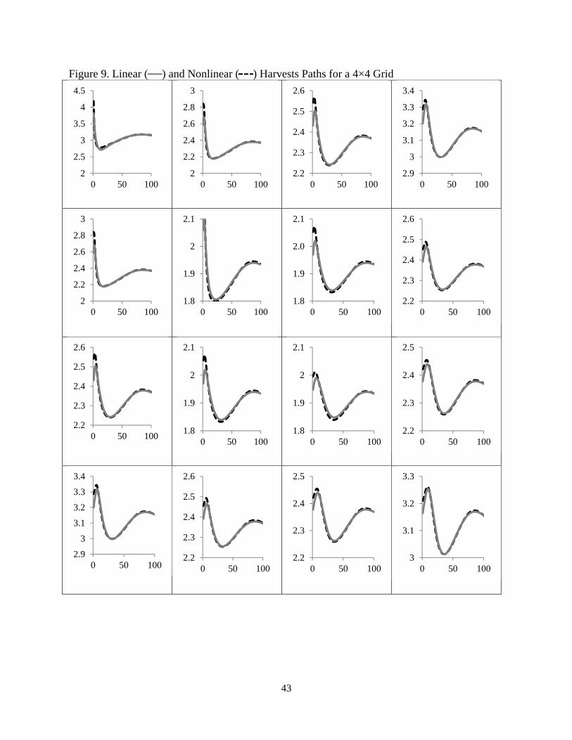
43  

Figure 9. Linear ( ) and Nonlinear ( ) Harvests Paths for a 4×4 Grid

2

2.5

3

3.5

4

4.5

0 50 1002

2.2

2.4

2.6

2.8

3

0 50 1002.2

2.3

2.4

2.5

2.6

0 50 1002.9

3

3.1

3.2

3.3

3.4

0 50 100

2

2.2

2.4

2.6

2.8

3

0 50 1001.8

1.9

2

2.1

0 50 1001.8

1.9

2.0

2.1

0 50 1002.2

2.3

2.4

2.5

2.6

0 50 100

2.2

2.3

2.4

2.5

2.6

0 50 1001.8

1.9

2

2.1

0 50 1001.8

1.9

2

2.1

0 50 1002.2

2.3

2.4

2.5

0 50 100

2.9

3

3.1

3.2

3.3

3.4

0 50 1002.2

2.3

2.4

2.5

2.6

0 50 1002.2

2.3

2.4

2.5

0 50 1003

3.1

3.2

3.3

0 50 100

44  

Figure 10. Comparison of Optimal Local Harvests with and without 2 effects

 Notes. The solid (dashed) lines represent adult tree harvesting under optimal local planning with (and without) the 2 endogenous migration term in (15). The vertical axis measures the number of adult trees harvested per acre on each local forest. The horizontal axis measures time in years. A MPB outbreak occurs in cell (1,1) at time 1 and is tracked for 50 years.

10 20 30 40 50

3.0

3.2

3.4

3.6

3.8Cell 1, 1

10 20 30 40 50

2.3

2.4

2.52.6

2.7

Cell 1, 2

10 20 30 40 50

2.6

2.7

2.8

2.9

Cell 1, 3

10 20 30 40 50

2.65

2.70

2.75

2.80

2.85

Cell 1, 4

10 20 30 40 50

2.35

2.40

2.45

Cell 1, 5

10 20 30 40 50

3.10

3.15

3.20

3.25Cell 1, 6

10 20 30 40 50

2.3

2.4

2.5

2.6

2.7

Cell 2, 1

10 20 30 40 50

1.9

2.0

2.1

Cell 2, 2

10 20 30 40 50

2.152.202.252.302.35

Cell 2, 3

10 20 30 40 50

2.15

2.20

2.25

2.30

Cell 2, 4

10 20 30 40 50

1.901.921.941.961.982.002.02

Cell 2, 5

10 20 30 40 50

2.35

2.40

2.45

Cell 2, 6

10 20 30 40 50

2.6

2.7

2.8

2.9

Cell 3, 1

10 20 30 40 50

2.152.202.252.302.35

Cell 3, 2

10 20 30 40 50

2.40

2.45

2.50

2.55

Cell 3, 3

10 20 30 40 50

2.40

2.45

2.50

2.55Cell 3, 4

10 20 30 40 50

2.142.162.182.202.222.242.26

Cell 3, 5

10 20 30 40 50

2.65

2.70

2.75

2.80Cell 3, 6

10 20 30 40 50

2.65

2.70

2.75

2.80

2.85

Cell 4, 1

10 20 30 40 50

2.15

2.20

2.25

2.30

Cell 4, 2

10 20 30 40 50

2.40

2.45

2.50

2.55Cell 4, 3

10 20 30 40 50

2.40

2.45

2.50

Cell 4, 4

10 20 30 40 50

2.162.182.202.222.242.26

Cell 4, 5

10 20 30 40 50

2.65

2.70

2.75

Cell 4, 6

10 20 30 40 50

2.35

2.40

2.45

Cell 5, 1

10 20 30 40 50

1.901.921.941.961.982.002.02

Cell 5, 2

10 20 30 40 50

2.142.162.182.202.222.242.26

Cell 5, 3

10 20 30 40 50

2.162.182.202.222.242.26

Cell 5, 4

10 20 30 40 50

1.901.92

1.941.96

1.982.00

Cell 5, 5

10 20 30 40 50

2.362.382.402.422.442.46

Cell 5, 6

10 20 30 40 50

3.10

3.15

3.20

3.25Cell 6, 1

10 20 30 40 50

2.35

2.40

2.45

Cell 6, 2

10 20 30 40 50

2.65

2.70

2.75

2.80Cell 6, 3

10 20 30 40 50

2.65

2.70

2.75

Cell 6, 4

10 20 30 40 50

2.362.382.402.422.442.46

Cell 6, 5

10 20 30 40 50

3.10

3.15

3.20

Cell 6, 6

45  

APPENDIX

Here, we present additional details on the calculation of the local and centralized harvesting

conditions, (11) and (14). We also discuss the choice of parameter values and a sensitivity

analysis to changes in the parameters.

Local first-order condition

The first-order condition for the fully forward-looking planner is

, 1 , , ∑,

,, , ∑ ∆ , , . (A1)

where ∆ , ,,

,

,

,

,

, is the effect of harvesting working through the seed

base. The harvesting condition in (11) therefore imposes two restrictions on the local manager’s

choice. First, the effect of harvesting on future MPB risk is limited to 1 and 2 effects.

This restricts the MPB migration and reproduction impacts from harvesting to neighboring

forests. Second, the seed effects of harvesting, ∆ , , are ignored. Due to the relatively slow

growth of the forest resource, these effects are negligible even when summed over the planning

horizon. For example, the seed effect in period 4, the first period a seed effect is present, is the

marginal net benefit of an adult tree in period 4 multiplied by less than 1 10 . All

subsequent seed effects are even smaller and at the boundaries of numerical precision.

The harvesting condition (11) involves two partial derivatives that capture the local manager’s

response to MPB risk. The first derivative is positive and given by

46  

,

,

,

,

,

,

, ,

, /

, → ,

, ,, ∑

, → ,

, ,,

∈ , 0    (A2) 

where

, → ,

, , 1 , → , ln 1 , → , 0(A3) 

, → ,

,

, → ,

, 1, → ,

, → , 0.                                      (A4) 

Equation (A2) reflects the ability of the manager on local forest , to harvest in period and

lower MPB risk in period 1 by encouraging migration off forest , and discouraging

migration to forest , .

The second derivative reflects the ability of the manager to harvest in period and influence

MPB risk in period 2:

, ,

, ,

, /

, → ,,

,,

, , ,

∑ , → ,,

,, → ,

, , → ,

,

, ,∈ ,

(A5)

where

,

, , ,

, /

, → ,

, ,, ∑

, → ,

, ,,

∈ (A6)

, → ,

, , ln 1 , → , , → ,                                 (A7)

47  

, → ,

,

, → ,

, , → , (A8)

, → ,

,

, → ,

,

,

,

,

, , → ,

,

,

,, (A9)

, → ,

, , ln 1 , → , , → , . (A10)

The index in (A6) runs over the set of neighbors shared by cell , and cell , . The

effect on , in (A5) occurs through both MPB reproduction and migration.

Central first-order condition

The central planner’s first-order condition includes two derivatives that account for the

spatial MPB externality. The first is given in (A6) and the second is

, ,

, ,

, /, → ,

,,

,

, , , , (A11)

Equations (A6) and (A11) are similar to equations (A2) and (A5) except rather than harvests

impacting own MPB risk, harvests impact MPB risk on neighboring forests.

Selection of the parameter values

In this section, we discuss the selection of the parameter values shown in Table 1. We set the

discount rate equal to 4% (implying a discount factor of 0.96) in accordance with USDA FS

practice (Row, et al., 1981). The parameters dictating seed production , ,

48  

germination , maturation , and natural mortality ( ) produce comparable and defensible

values for typical USDA FS land in the western U.S. (Koch, 1996). These forest-specific

parameters also allow the forest to re-establish within 80 to 140 years following a stand-

replacing disturbance (Lotan and Critchfield, 1990).

MPB-specific parameters , , and depend on site conditions, tree species, climate, and

geography among other things. Proportional changes in and have little impact on the model.

The key value is the ratio of tree resistance to beetle fecundity, / . Previous studies provide

multiple measures of the fecundity of an infested tree by counting the number of emerging

beetles (e.g., Bentz, 2006). These studies generally place between 4,000 and 5,000 beetles per

infested tree. There have been few studies that have investigated ; however, indirect measures

of this parameter can be obtained by combining various field measurements. For example,

Heavilin and Powell (2008) find that the parameter should lie between 56,000 and 240,000

beetles per acre based on attack density measures from Berryman, Dennis, Raffa, and Stenseth

(1985) and forest structure measures from Cole and McGreggor (1983). Using more recent

aerial survey data from 1990 to 2001 and an estimating function procedure, Heavilin and Powell

(2008) find that the ratio / may range from 1.6 to 16.2 trees per acre. This suggests should

lie between 6,478 and 80,972 beetles per acre. Our choice of a = 63,800 is within the ranges

implied by both approaches. Finally Berryman et al. (1985) report a decreasing relationship

between MPB offspring and the number of MPB attacks per square meter of tree surface area.

This indicates decreasing reproductive returns from increases in adult-tree mortality and implies

a degree of curvature in (9). In the absence of any additional quantitative results to guide us, we

set 0.5.

49  

The non-timber preference parameter is set at 6.23, which is selected to ensure an

average steady-state harvest per acre of 2.5. The selected value is consistent with USDA FS

data showing average harvests in MPB habitat to range from 0.008% to 3.2% of the total

inventory of adult pine trees (Smith, et al., 2009). Setting average harvests at 2.5 implies a

harvest level equal to 1% of the adult tree stock, an approximate midpoint of this range.

The dispersal parameters, and determine the shape and position of the MPB dispersal

function. Since MPB may only disperse at a rate of one cell per year, the appropriate choice for

and is dependent on the size of the cells relative to the scale of beetle dispersal. Research

shows that MPB can disperse as far as 250 meters via flight migration (Safranyik, et al., 1992)

with the possibility of longer-range wind dispersal on the order of tens and hundreds of

kilometers (Safranyik and Carroll, 2006). With so much variation in the scale of MPB dispersal,

it is difficult to define the relationship between these parameters and cell size.13 In order to move

forward, we set 10 and specify forest-specific values for that range between 0.0037

and0.0059. The chosen values for and produce a dispersal function, , → , , such that

50% of the beetles migrate to adjacent cells at the local planner steady state (see figure 2). We

experiment with alternative steady-state values of , → , ; results are reported below.

Sensitivity Analysis to Parameter Changes

Table A1 shows the steady-state values for a change in several fundamental parameters.

Each parameter is individually decreased and increased from its value in Table 1. Drought and                                                             13 In future research, we intend to more accurately measure the size and shape of each local forest using GIS mapping techniques. Each local forest will be mapped and divided into multiple spatial cells that will allow more precision in modeling MPB dispersal within and across local forests. This is an area for future research but beyond the scope of the current paper.

50  

winter temperatures can cause changes in the number of MPB offspring from an infested tree ( )

and tree defenses against MPB attack ( ) (Heavilin and Powell, 2008). An increase in leads to

more killed trees and fewer MPB. Even though more MPB emerge from an infested tree, there

are fewer host trees so the MPB population falls. Likewise, a decrease in implies that a tree’s

defenses have weakened and fewer MPB are needed to successfully attack a tree. This results in

fewer trees and fewer MPB. In both cases, the reproduction externality increases relative to the

migration externality because failure to harvest a tree results in more successful MPB

reproduction, which, in turn, increases MPB migration to neighboring forests. An increase in

can be interpreted as a less healthy forest with a higher natural death rate. This leads to less

harvesting, fewer trees and fewer MPB. The reproduction externality now exceeds the migration

externality because the migration externality is smaller due to the reduction in the MPB

population. This implies that recent changes in climate and forest health will provide an

incentive for local managers to under-harvest as a result of the spatial externality. In contrast, an

increase in implies a greater preference for non-timber forest benefits and therefore less

harvesting, more trees, more MPB, and a relatively greater migration externality. Finally,

, → , determines how many MPB migrate off the local forest in steady state. We fix this

value at 0.5 for each local forest. Although changes in , → , have little effect on the steady-

state values, we note that they have a significant effect on the spread of a MPB outbreak over the

forest landscape.

51  

Table A1. Sensitivity Analysis to Parameter Changes

Parameter % Change Variable (under Optimal Central Planning)

net externality

(migration + reproduction)

5%† 2.43 225.55 3754.41 0.0021

0% 2.46 203.40 2943.89 0.0013

+5%† 2.49 184.32 1683.07 0.0004

ν

3%† 2.47 196.17 2530.57 -0.0010

0% 2.46 203.40 2943.89 0.0013

+3%† 2.45 207.73 3158.53 -0.0014

10% 2.41 171.56 772.44 +0.0001

0% 2.46 203.40 2943.89 0.0013

+10% 2.41 246.44 4699.13 0.0028

10% 2.56 203.24 2560.85 0.0009

0% 2.46 203.40 2943.89 0.0013

+10% 2.40 203.33 3152.95 0.0015

10% 2.42 203.76 4227.26 0.0027

0% 2.46 203.40 2943.89 0.0013

+10% 2.32 201.26 1630.26 +0.0001

, → ,

10% 2.47 203.79 2919.78 0.0010

0% 2.46 203.40 2943.89 0.0013

+10% 2.44 203.04 2965.35 0.0016

Notes. The variables are measured as the average steady-state values across the 36 cells on the landscape forest grid. The net spatial externality is given by equation (14). A negative number indicates that the migration externality (first term in equation (14)) dominates the reproduction externality (second term in equation (14)). A positive value indicates that the reproduction externality dominates the migration externality. (†) Steady-states could not be found for 10% changes in and ν.