Spatial coherence of sunlight and itsimplications for light management inphotovoltaicsSHAWN DIVITT AND LUKAS NOVOTNY*Photonics Laboratory, ETH Zürich, 8093 Zürich, Switzerland

*Corresponding author: lnovotny@ethz.ch

Received 14 August 2014; revised 12 December 2014; accepted 12 December 2014 (Doc. ID 221013); published 27 January 2015

New technologies are emerging that capture and redirect sunlight inside solar cells. This type of light man-agement can significantly increase efficiency, but the device behavior will fundamentally depend on thespatial coherence of the incoming light. This dependence calls for a complete characterization of the spatialcoherence of sunlight. Here, we present the first spectral measurements of the spatial degree of coherence ofdirect, diffuse, and simulated sunlight. An expression is derived for both the cross-spectral density and thespatial degree of coherence in an arbitrarily oriented device plane, including the effects of overcast skies.Implications of the present work are discussed and may lead to a better understanding of light-managingcomponents in solar cells as well as a new class of solar simulator that provides both the same spectrum andspatial coherence as direct sunlight. © 2015 Optical Society of America

OCIS codes: (030.1640) Coherence; (350.6050) Solar energy; (030.1670) Coherent optical effects.

http://dx.doi.org/10.1364/OPTICA.2.000095

1. INTRODUCTION

Multi-junction solar cells, which divide or selectively respondto portions of the solar spectrum, are the highest-efficiencycells ever produced [1]. However, spectral control is only apartial solution toward maximizing efficiency [2]; a comple-mentary method for higher performance is the use of light-managing structures that capture or redirect light [3–12].

Light management can increase efficiency in single- andmulti-junction cells, but the device behavior will depend onboth the spatial coherence and the bandwidth of the incominglight [13]. The behavior of rectenna solar cells has similardependencies [14,15]. It is therefore necessary to fully charac-terize the spectral variation of the spatial coherence of sunlight.We refer to devices whose behavior depends on spatial coher-ence as coherent photovoltaics or co-PVs.

The spatial coherence of direct terrestrial sunlight (sun-shine) was first considered in the 19th century by Verdet[16]. Much more recently the machinery of modern coherencetheory was applied to the calculation of the spectral degree ofspatial coherence expected from sunshine by Agarwal et al. [17]

and found to essentially match Verdet’s expectation. Indeed,the mutual intensity of sunshine, a broadband quantity that isrelated to the spectral degree of coherence [18], was sub-sequently measured by Mashaal et al. [19] and found to sub-stantially agree with the expectation [20]. However, thecalculations of Agarwal et al. are based on a uniform spheremodel and therefore ignore real optical effects such as solarlimb darkening.

While the previous measurements demonstrate agreementwith the theory in the broadband case, the spectral degree ofcoherence, which considers each spectral component sepa-rately, has not been measured. Further, if co-PVs are to be usedin real applications, it is necessary to understand the spatialcoherence of sunlight under non-ideal weather conditions aswell as to establish a spatial coherence standard for device test-ing. Here, we present the first interferometric measurements ofthe transverse spectral degree of coherence of both direct sun-shine and diffuse terrestrial sunlight, where the Sun is obscuredby clouds or fog. In this context, transverse indicates that thecoherence function is measured in a plane whose normal vectorpoints directly toward the center of the Sun.

2334-2536/15/020095-09$15/0$15.00 © 2015 Optical Society of America

Research Article Vol. 2, No. 2 / February 2015 / Optica 95

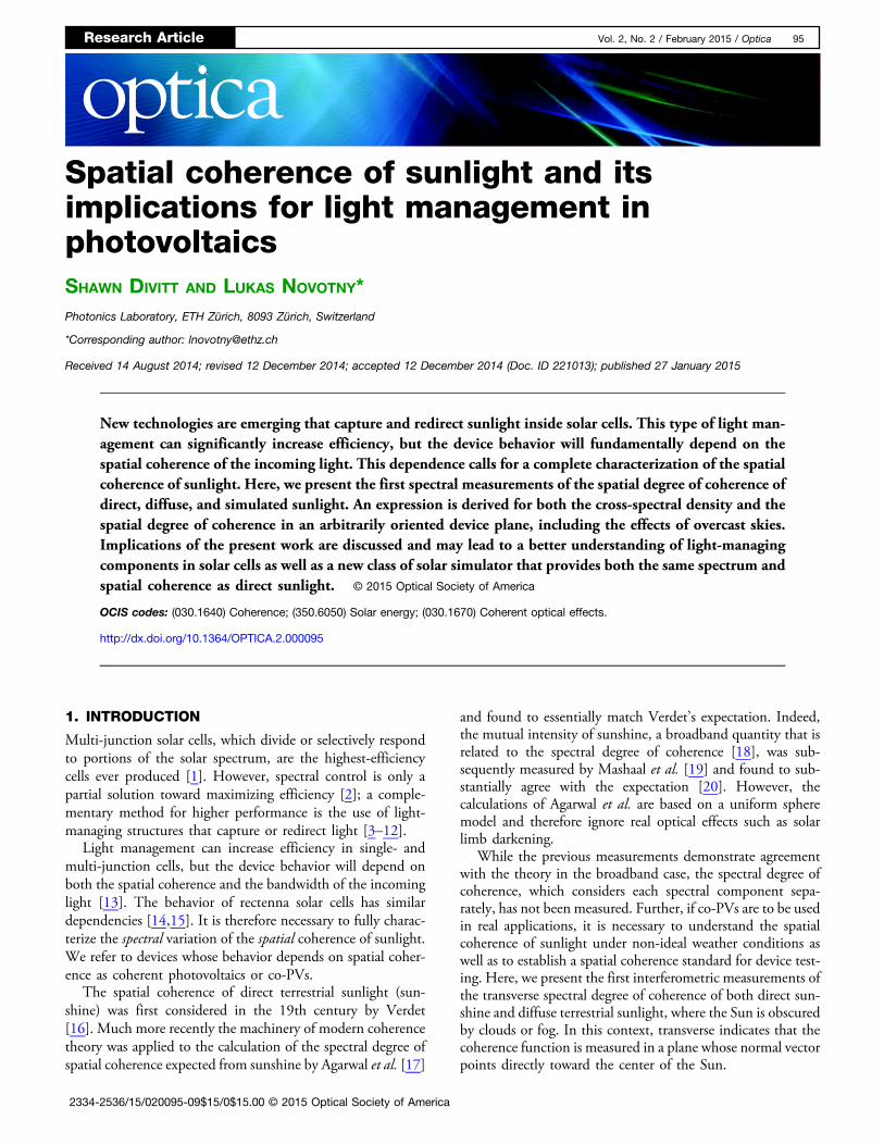
Our measurements are performed using the method illus-trated in Fig. 1. The method involves non-parallel slits and itsworking principles have been described previously [21]. Themeasurements are precise enough to distinguish betweenthe expectations of uniform and limb-darkened incoherentspheres. To demonstrate the precision of the measurements,we compare our findings with those expected by theory as ap-plied to hyperspectral solar limb darkening measurementsmade by Neckel and Labs [22]. We also present a measure-ment of the spectral degree of coherence of light emitted bya solar simulator, establishing the need for a spatial coherencestandard in co-PV device testing.

To provide context to the measurements and their practicaluse, we present the theory of the spectral degree of coherenceof sunlight beyond the transverse case and/or under a uni-formly cloudy sky. Unless sophisticated tracking methodsare used, a photovoltaic cell is generally never in a plane whosenormal vector points directly toward the center of the Sun.Consequently, a description of how the coherence propertiesof sunlight vary with the position of the Sun in the sky relativeto a fixed device plane is important to predict the behavior ofco-PVs at different times in the day. We provide an expressionthat derives any non-transverse spectral degree of coherencefunction in terms of the measured transverse function. Havingestablished these results, we discuss how to apply them to thesimulation of co-PV devices.

2. PROBLEM STATEMENT

Spatial coherence is a measure for the correlation between op-tical fields in different locations of space. More specifically, weare interested in measuring the degree of spatial coherence,η�r1; r2;ω�, which gives a scalar description of the statisticalcorrelation between the fields with frequency ω at locationsr1 and r2. In the following we will refer to η�r1; r2;ω� asthe spectral degree of coherence [23]. In general, a degreeof coherence can be described between any pair of field com-ponents for any pair of points in space. A rigorous descriptionof second-order coherence is given by a 3 × 3 covariance matrixknown as the cross-spectral density (CSD) matrixW�r1; r2;ω�(see Mandel and Wolf [24], Sect. 6.6.1). The CSD matrix isdirectly applicable to the numerical simulation of light propa-gating in a solar cell (see Implications). However, the spectral

degree of coherence can be more easily measured and providesevidence for the structure of a theoretical CSD matrix.

The spectral degree of coherence can be defined in terms ofthe CSD matrix as [23]

η�r1; r2;ω�≔Tr�W�r1; r2;ω��ffiffiffiffiffiffiffiffiffiffiffiffiffiffiffiffiffiffiffiffiffiffiffiffiffiffiffiffiffiffi

Tr�W�r1; r1;ω��p ffiffiffiffiffiffiffiffiffiffiffiffiffiffiffiffiffiffiffiffiffiffiffiffiffiffiffiffiffiffi

Tr�W�r2; r2;ω��p ; (1)

where Tr denotes the matrix trace. The two-slit apparatus illus-trated in Fig. 1 provides a simple and robust measurement of ηas defined by Eq. (1) (see Appendix A). We note that alterna-tive definitions of the spectral degree of coherence exist thattake all elements of W into account [25]. However, the useof Eq. (1) is justified by the facts that direct and cloud-diffusedsunlight are unpolarized [26] and therefore Eq. (1) representsthe essential elements of W. Partially polarized skylight (bluesky) is discussed as a separate case in Appendix E.

For scalar fields, the van Cittert-Zernike theorem has beentraditionally used to calculate the CSD of sunshine (see Bornand Wolf [27], Sect. 10.4.2). For electromagnetic fields, thegeneral case can be calculated using an angular spectrum ofplane waves propagating within a solid angle σ subtended bythe source at the device plane. Under the assumption ofangularly uncorrelated and unpolarized plane waves theCSD matrix is given by [28,29]

W�r1; r2;ω�≔hE��r1;ω�E⊺�r2;ω�i

�Zσa�u;ω��U3 − uu⊺� exp�iku · r�dΩ; (2)

where E is the random electric field column vector;

u � − sin θ cos ϕx − sin θ sin ϕy − cos θz

is the unit vector that specifies the propagation direction of aplane wave (θ and ϕ represent polar and azimuthal sphericalcoordinates, respectively); the vectors j�j � x; y; z� are the unitcolumn vectors along the coordinate axes (see Fig. 2(a));dΩ≔ sin θdθdϕ is the differential solid angle; k≔ω∕c is thewavenumber; r≔r2 − r1; U3 is the 3 × 3 identity matrix;a�u;ω� is, up to a constant, the average power spectral densityper unit solid angle of waves traveling with frequency ω in theu direction; � indicates complex conjugate; ⊺ indicates vectortranspose; and the angle brackets indicate an ensembleaverage over monochromatic field realizations. Equation (2)immediately implies, under the given assumptions, thatW�r1; r1;ω� � W�r2; r2;ω� and that W�r1; r2;ω� is a func-tion of r alone such that we can write W�r ;ω� and η�r ;ω�in their respective places. For a very distant source, the func-tion a�u;ω� is given by the power spectral density distributionof the source that is apparent from the origin (see Novotny andHecht [30], Sect. 3.4).

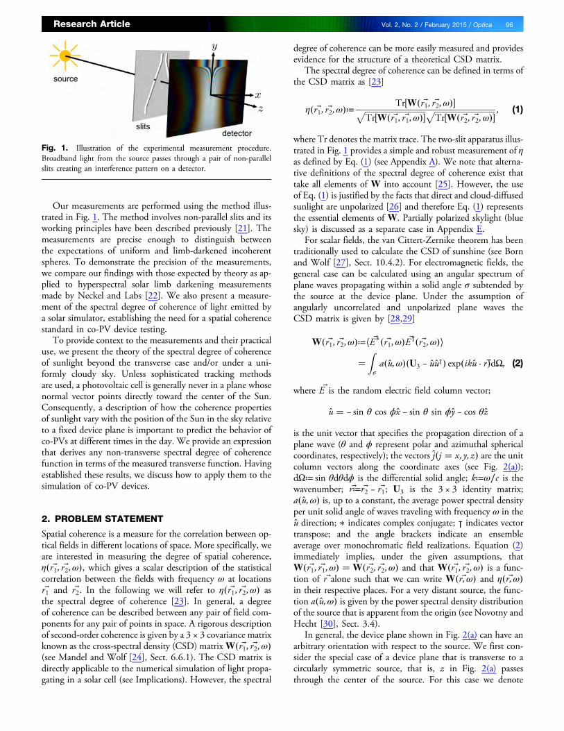
In general, the device plane shown in Fig. 2(a) can have anarbitrary orientation with respect to the source. We first con-sider the special case of a device plane that is transverse to acircularly symmetric source, that is, z in Fig. 2(a) passesthrough the center of the source. For this case we denote

Fig. 1. Illustration of the experimental measurement procedure.Broadband light from the source passes through a pair of non-parallelslits creating an interference pattern on a detector.

Research Article Vol. 2, No. 2 / February 2015 / Optica 96

the spectral degree of coherence as η⊥, or the transverse spectraldegree of coherence. Due to rotational symmetry, η⊥�r ;ω� is afunction of r≔jrj alone and can be written η⊥�r;ω�. Later, wewill consider an arbitrarily oriented device plane and express ηin terms of η⊥ and orientational angles.

In the following we will distinguish between two differenttypes of sources, direct sunshine and diffuse sunlight. Thelatter corresponds to a uniformly bright, cloudy sky. We modelthis situation with a spatially incoherent half-shell sourcewhose radius is large, surrounding the device plane (seeFig. 2(b)). The origin of the device plane is placed at the centerof the half-shell. The spectral degree of coherence in this case isgiven by (see Appendix B) [23,31]

ηs�r ;ω� �sin�kjrj�kjrj : (3)

This result indicates that, for a spatially incoherent half-shellsource, the spatial coherence length along any direction at thecenter of the shell is on the order of one wavelength ofthe light.

Light illuminating the device plane is in general a mixture ofdirect and diffuse sunlight. We model this situation as thecombination of a disk and a half-shell source, as shown inFig. 2(b). Consequently, the spectral degree of coherence isgiven by (see Appendix C)

η�r ;ω� � sdsd � ss

ηd �r ;ω� �ss

sd � ssηs�r ;ω�; (4)

where sd and ss represent the spectral densities in the deviceplane due to the disk and shell, ηs is given by Eq. (3) andηd is the spectral degree of coherence in the disk-only caseas defined by Eqs. (1) and (2). Introducing the parameterγ≔sd∕�sd � ss�, we can rewrite the equation above as

η�r ;ω� � γηd �r ;ω� � �1 − γ�ηs�r ;ω�: (5)

In the next section we will use a simple experimental pro-cedure to measure η in the transverse plane and compare theresults with the theoretical model, Eq. (5).

3. EXPERIMENTAL RESULTS

We have fabricated a pair of non-parallel slits to measure thetransverse spectral degree of coherence of i) direct sunshine, ii)light emitted by a solar simulator, and iii) diffuse sunlight (seeAppendix A for materials and methods).

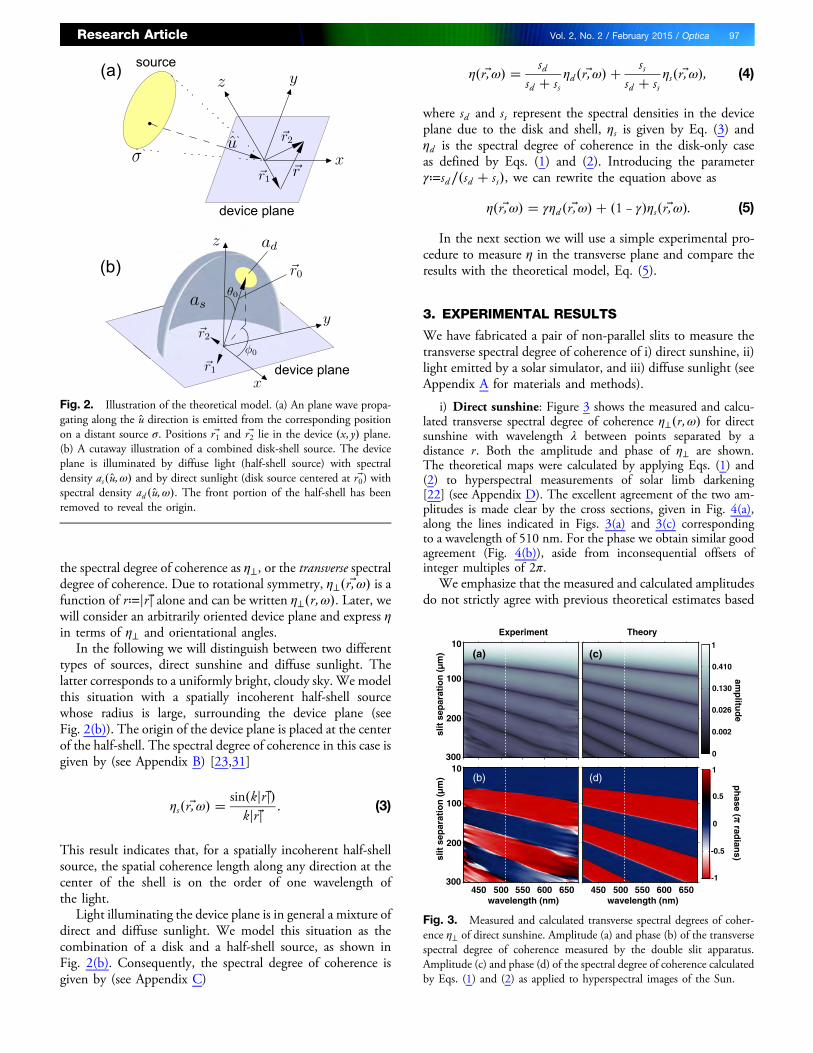
i) Direct sunshine: Figure 3 shows the measured and calcu-lated transverse spectral degree of coherence η⊥�r;ω� for directsunshine with wavelength λ between points separated by adistance r. Both the amplitude and phase of η⊥ are shown.The theoretical maps were calculated by applying Eqs. (1) and(2) to hyperspectral measurements of solar limb darkening[22] (see Appendix D). The excellent agreement of the two am-plitudes is made clear by the cross sections, given in Fig. 4(a),along the lines indicated in Figs. 3(a) and 3(c) correspondingto a wavelength of 510 nm. For the phase we obtain similar goodagreement (Fig. 4(b)), aside from inconsequential offsets ofinteger multiples of 2π.

We emphasize that the measured and calculated amplitudesdo not strictly agree with previous theoretical estimates based

Fig. 2. Illustration of the theoretical model. (a) An plane wave propa-gating along the u direction is emitted from the corresponding positionon a distant source σ. Positions r1 and r2 lie in the device �x; y� plane.(b) A cutaway illustration of a combined disk-shell source. The deviceplane is illuminated by diffuse light (half-shell source) with spectraldensity as�u;ω� and by direct sunlight (disk source centered at r0) withspectral density ad �u;ω�. The front portion of the half-shell has beenremoved to reveal the origin.

(d)

(c)

(b)

(a)

Experiment Theory

wavelength (nm)450 500 550 600 650

1

0.5

0

-0.5

-1

1

0.410

0.130

0.026

0.002

0

amp

litud

ep

hase (

radian

s)

wavelength (nm)450 500 550 600 650

slit

sep

arat

ion

(µ

m)

slit

sep

arat

ion

(µ

m)

10

100

200

30010

100

200

300

Fig. 3. Measured and calculated transverse spectral degrees of coher-ence η⊥ of direct sunshine. Amplitude (a) and phase (b) of the transversespectral degree of coherence measured by the double slit apparatus.Amplitude (c) and phase (d) of the spectral degree of coherence calculatedby Eqs. (1) and (2) as applied to hyperspectral images of the Sun.

Research Article Vol. 2, No. 2 / February 2015 / Optica 97

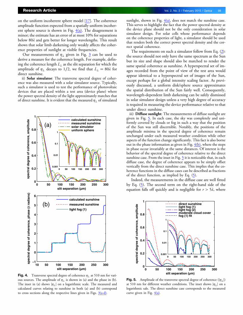
on the uniform incoherent sphere model [17]. The coherenceamplitude function expected from a spatially uniform incoher-ent sphere source is shown in Fig. 4(a). The disagreement isminor; the estimate has an error of at most 10% for separationsbelow 80λ and gets better for longer wavelengths. This resultshows that solar limb darkening only weakly affects the coher-ence properties of sunlight at visible frequencies.

Our measurements of η⊥ given in Fig. 3 can be used toderive a measure for the coherence length. For example, defin-ing the coherence length L⊥ as the slit separation for which theamplitude of η⊥ decays to 1∕2, we find that L⊥ � 80λ fordirect sunshine.ii) Solar simulator: The transverse spectral degree of coher-

ence was also measured with a solar simulator source. Typically,such a simulator is used to test the performance of photovoltaicdevices that are placed within a test area (device plane) wherethe power spectral density of the light approximately matches thatof direct sunshine. It is evident that the measured η⊥ of simulated

sunlight, shown in Fig. 4(a), does not match the sunshine case.This serves to highlight the fact that the power spectral density atthe device plane should not be the only consideration in solarsimulator design. For solar cells whose performance dependson the coherence properties of light, a simulator should be usedthat renders both the correct power spectral density and the cor-rect spatial coherence.

The requirements on such a simulator follow from Eq. (2):the source should not only have the same spectrum as the Sunbut its size and shape should also be matched to render thesame spatial coherence as sunshine. A hyperspectral set of im-ages recorded from the point of view of the test area wouldappear identical to a hyperspectral set of images of the Sun,except perhaps for a global intensity scaling factor. As previ-ously discussed, a uniform disk/sphere source approximatesthe spatial distribution of the Sun fairly well. Consequently,wavelength-dependent limb darkening can be safely dismissedin solar simulator design unless a very high degree of accuracyis required in measuring the device performance relative to thatunder direct sunshine.iii) Diffuse sunlight: The measurements of diffuse sunlight are

given in Fig. 5. In each case, the sky was completely and uni-formly covered by clouds or fog in such a way that the positionof the Sun was still discernible. Notably, the positions of theamplitude minima in the spectral degree of coherence remainunchanged under each measured weather condition while otheraspects of the function change significantly. This fact is also borneout in the phase information as given in Fig. 4(b), where the stepsin phase occur invariably at the same distances. Of interest is thebehavior of the spectral degree of coherence relative to the directsunshine case. From the inset in Fig. 5 it is noticeable that, in eachdiffuse case, the degree of coherence appears to be simply offsetvertically from the direct sunshine case. This implies that the co-herence functions in the diffuse cases can be described as fractionsof the direct function, as implied by Eq. (5).

Indeed, the measurements in the diffuse case are well fittedby Eq. (5). The second term on the right-hand side of theequation falls off quickly and is negligible for r > 5λ, where

0 50 100 150 200 250 3000

0.2

0.4

0.6

0.8

1

slit separation (µm)

spec

tral

deg

ree

of

coh

eren

ce, a

mp

litu

de

(a)

0 50 100 150 200 250 3000.001

0.01

0.1

1

calculated sunshinemeasured sunshinesolar simulatoruniform sphere

10 50 100 150 200 250 300−1

0

1

2

3

4

5

6

slit separation (µm)

spec

tral

deg

ree

of

coh

eren

ce, p

has

e (

rad

ian

s)

(b)calculated sunshine

measured sunshine

light fog (1)

Fig. 4. Transverse spectral degree of coherence η⊥ at 510 nm for vari-ous sources. The amplitude of η⊥ is shown in (a) and the phase in (b).The inset in (a) shows jη⊥j on a logarithmic scale. The measured andcalculated curves relating to sunshine in both (a) and (b) correspondto cross sections along the respective lines given in Figs. 3(a-d).

0 50 100 150 200 250 3000

0.2

0.4

0.6

0.8

1

slit separation (µm)

spec

tral

deg

ree

of

coh

eren

ce, a

mp

litu

de

0 50 100 150 200 250 3000.001

0.01

0.1

1

direct sunshinelight fog (1)light fog (2)moderate cloud coverfog (1) fit

Fig. 5. Amplitude of the transverse spectral degree of coherence (jη⊥j)at 510 nm for different weather conditions. The inset shows jη⊥j on alogarithmic sale. The direct sunshine case corresponds to the measuredcurve given in Fig. 4(a).

Research Article Vol. 2, No. 2 / February 2015 / Optica 98

r � jr2 − r1j is the distance between points in the transverseplane. Then, ignoring the second term, Eq. (5) can be approxi-mated by γη⊥�r;ω�. Thus, the simple relationship betweenthe diffuse cases and the direct function becomes clear.This approximation was used with a value γ � 0.45 infitting the first fog case. The fit and measurement overlapsignificantly.

The second fog measurement was taken two minutes afterthe first using a slightly different system (see Appendix A). Inthis case, a peak-like feature related to the second term on theright-hand side of Eq. (5) becomes visible in the lowest slitseparation region. This feature is significantly wider than ex-pected by the second term. The discrepancy between the sec-ond fog measurement and the second term in Eq. (5) is duesimply to the fact that the diffused light was not truly uniform.In reality, the brightness of the fog fell off for positions awayfrom the Sun. This factor effectively narrowed the spatial dis-tribution of the source and thus widened the part of the co-herence function due to diffused light. However, even giventhis discrepancy, it is clear that the spatial coherence lengthis greatly reduced in the diffuse case as compared to the directsunshine case. For example, using the same definition for thecoherence length L⊥ as before, we find for the second fog caseL⊥ � 7λ as given by Fig. 5. This length is expected by Eq. (5)to be as low as λ∕3 in the extreme (γ � 0) case.

4. ARBITRARILY ORIENTED DEVICE PLANE

We proceed by describing how, in the solar disk-only case, thecross spectral density Wd �r1; r2;ω� and spectral degree of co-herence ηd �r1; r2;ω� between points in an arbitrarily orienteddevice plane can be given in terms of the transverse functionsW⊥�r ;ω� and η⊥�r;ω�, where r≔r2 − r1 and r≔jrj. We as-sume a spatially incoherent, broadband source that appears cir-cularly symmetric (but not necessarily uniform) from theorigin. We define the set of rectangular coordinate axesx; y; z such that r1 and r2 lie in the x–y plane and the centerof the source is located at position r0, with polar angle θ0 andazimuthal angle ϕ0 (see Fig. 2(b)). We assume that the sourceis far from the device plane such that jr0j is much larger than r.

Now, by applying the appropriate rotation matrix to thecross-spectral density in the transverse case, we can find thecross-spectral density and spectral degree of coherence betweenany two points in the device plane. Let M�θ0;ϕ0�≔Rz�ϕ0�Ry�θ0� where Ri�φ� is a rotation about the i axis byangle φ as given by the right-hand rule. Then, as shown explic-itly in Appendix D, Wd and ηd can be expressed as

Wd �r1; r2;ω� ≈MW⊥�M⊺r ;ω�M⊺ exp�−ikrp�; (6)

and

ηd �r1; r2;ω� ≈ η⊥�rffiffiffiffiffiffiffiffiffiffiffi1 − p2

q;ω� exp�−ikrp�; (7)

where p≔ sin θ0 cos�ϕ0 − ϑ�, ϑ≔ arctan�r · y; r · x�, andarctan�y; x� is the four-quadrant inverse tangent. The functionsW⊥�r ;ω� and η⊥�r;ω� describe, respectively, the cross-spectraldensity and spectral degree of coherence in the transverse plane

(the θ0 � 0, sunshine-only case), the latter of which is given inFig. 3. We note that the degree of coherence between points inthe transverse plane is a function of only ω and the distance rbetween the points; fields of this type are known as Schell-model fields [32].

Coherence functions in the general case: We now con-sider a device plane that is oriented obliquely to the transverseplane and illuminated by both diffuse and direct sunlight. Asbefore, we model this situation as the combination of a diskand a half-shell (see Fig. 2(b)).

By the additive nature of the cross-spectral density formutually-incoherent sources, and by Eqs. (3), (5), (6), and(7) we find

W�r1; r2;ω� ≈Wd �r1; r2;ω� �Ws�r1; r2;ω�; (8)

and

η�r1; r2;ω� ≈ γη⊥�rffiffiffiffiffiffiffiffiffiffiffi1 − p2

q;ω�e−ikrp � �1 − γ� sin�kr�

kr; (9)

where Ws is the cross-spectral density in the device plane dueto the uniform half-shell (explicit expressions for W⊥ and Wsare given in Appendix D).

Equations (8) and (9) are the main results of this section.They state that the cross-spectral density and spectral degree ofcoherence between two points in a device plane can be de-scribed by their relative distance (r), their orientation with re-spect to the Sun (θ0;ϕ0; ϑ), the transverse coherence functionsof direct sunshine (W⊥, η⊥), the frequency (ω), and the ratio(γ) between the spectral densities in the device plane due to theSun and a uniform cloud cover or fog. Using Eq. (9)together with our experimental results for η⊥ we can derivethe spectral degree of coherence in an arbitrarily orienteddevice plane.

5. IMPLICATIONS FOR THE SIMULATION OFCOHERENT PHOTOVOLTAICS

In general, the electromagnetic field impinging on a device isnot a plane wave but rather it fluctuates randomly in time andspace. The average response of a device is thereby an ensembleaverage of responses to random field realizations. In simulatingdevices, it is not enough to consider the response under planewave illumination; a rigorous treatment requires that they besimulated under realizations of the full field. The cross-spectraldensity matrix W is a particular measure for the statistics ofthese realizations. In fact, W as given by Eq. (8) can beused to directly generate realizations of the field [33]. Anothermethod for generating realizations, as implied by Eq. (2), is touse a Monte Carlo simulation in which plane waves with ran-dom polarization, phase, and wave vector are coherentlysuperposed.

For devices with a linear response, the requirements for real-istic simulations become more relaxed. For some ensembleaveraged observable B�ω� (absorption, external quantum effi-ciency, etc.), we can write [34]

Research Article Vol. 2, No. 2 / February 2015 / Optica 99

B�ω� �Zσa�u;ω�χ�u;ω�dΩ; (10)

where a, σ, and dΩ are as before (see Problem Statement andAppendix D). χ is the generalized linear susceptibility that cor-responds to the observable B and describes the response of thesystem to unpolarized plane waves traveling in the u directionwith frequency ω. Simply, the device can be simulated underillumination by plane waves of different wave vectors andpolarizations and the responses to these waves can belinearly summed with the proper weight to determine theoverall response. Implementation of Eq. (10) is therefore com-patible with simulation modalities that consider plane waveillumination.

It is also possible, from knowledge of the dielectric suscep-tibility of the scattering medium and the CSDmatrixW of theincoming light, to determine the power spectral density distri-bution of light within a device. Such a calculation would in-volve propagating W into the device [13,35] and using thebasic equations for scattering in random media (see Mandeland Wolf [24], Sect. 7.6) to determine the power spectrum.

6. CONCLUSIONS

We have used a double slit aperture, in which the slit separa-tion slowly varies, to measure the transverse spectral degree ofcoherence of direct sunshine, sunlight diffused by clouds orfog, and light emitted by a solar simulator. The results in thedirect case were compared to those expected by theory asapplied to hyperspectral image data and found to agree.The results are precise enough to distinguish the true transversespectral degree of coherence of direct sunlight from the uni-form disk approximation. It was shown that, in general, theuniform disk approximation is very close to the measuredfunction.

We have shown that the spectral degree of coherence in aplane that is arbitrarily oriented with respect to a circularlysymmetric source, such as the Sun, can be derived given thetransverse spectral degree of coherence. A simple model wasalso developed to describe the spectral degree of coherenceunder overcast skies. This model was shown to accurately fitthe diffuse sunlight measurements in the transverse case. Fur-ther, an intuitive set of requirements was provided for the de-sign of a solar simulator with spatial coherence propertiessimilar to those of the Sun.

We have also described a method by which simulations ofco-PVs can include the effects of partial coherence. For lineardevices, an ensemble average of plane wave responses is suffi-cient. For non-linear devices, a rigorous treatment includes anensemble average of the device response to random realizationsof the field. We have also shown that, for devices with effectivedimensions on the order of a few wavelengths or less, directsunlight can be approximated as spatially coherent. However,this is not true for overcast skies where the coherence functionfalls off quickly within these dimensions. This implies that fu-ture co-PV designs should take into account the spatial coher-ence of sunlight, especially if the components are expected tobe used under cloud cover. Additionally, co-PVs should be

tested under a spatial coherence standard such that fair com-parisons may be made between different devices.

APPENDIX A: MATERIALS AND METHODS

Measurement apparatus: The measurement procedure hasbeen described previously in Ref. [21]. The measurementswere performed using a stock Nikon DX-format camera sensorplaced at a distance of 6.19 cm behind non-parallel slits, asshown in Fig. 1. The slit separation varies from 10 to 300 μm.6.19 cm is sufficient to be in the far-field of the two slits to-gether but still in the near-field of the long dimension of eachslit. Consequently, diffraction can be approximated as takingplace only along the direction that connects the two slits andthe resulting interference pattern describes an ensemble of si-multaneous Thompson-Wolf experiments [36]. The spectraldegree of coherence is recovered by combining informationfrom the interference pattern with power spectra as measuredby the same device. Technically, Ref. [21] provides a methodto measure the spectral degree of coherence μ�r1; r2;ω� of ascalar field. However, under comparison with Ref. [23], itis clear that the same method measures the spectral degreeof coherence η�r1; r2;ω� of an electromagnetic vector field.

Direct sunlight: Our measurement of direct sunlight wasperformed by recording only two images, one to measure thespectrum and one to measure the spectral degree of coherence.The first image, to measure the spectrum, is of an interferencepattern created by illuminating the slits with sunshine reflectedfrom a small, distant mirror. The second image is of an inter-ference pattern created behind the aperture by direct sunshine.By using the first image to normalize the second, as describedin [21], the transverse spectral degree of coherence can be mea-sured. The measurement was made on 22 March 2013 inZurich, Switzerland. A solar semi-diameter of 16.1 minutes,corresponding to 15 March 2013 [37], was used in the calcu-lation of the theoretical maps. The uniform disk source calcu-lation was also made assuming a 16.1 minute semi-diameter.

Solar simulator: The simulator consists of a xenon arc-lamp with air-mass 1.5 optical filters. Our measurementmethod for the solar simulator source is similar to that of thedirect sunshine case. The coherence image was recorded at thedevice plane and the spectral image was recorded at a distanceof 2 m from the source. Further, since the simulator sourcesubtended a significant solid angle at the device plane, an extrapost-processing step was required beyond those described in[21]: the spectral image was deconvolved from the coherencefunction image. This allowed for the retrieval of the point-spread function that, when projected along one dimensionand convolved again with the spectrum image, gives the resultthat would be expected in the limit of very long slits and aSchell-model coherence function. The lowest spatial frequencycomponents of the point-spread function were obscured in theparticular images that were recorded. These components wererecovered by extrapolation using a polynomial fit of higher fre-quency components.

Diffuse sunlight: For diffuse sunlight we chose a simplermeasurement procedure. The transverse spectral degree ofcoherence corresponding to a wavelength of 510 nm was

Research Article Vol. 2, No. 2 / February 2015 / Optica 100

obtained by recording only a single image. The slits wereplaced behind a narrow-band-pass optical filter centered at510 nm and the equal time degree of coherence j����r� wasfound using the method described in [21] and directly equatedto the spectral degree of coherence via an equation first derivedby Wolf [38]: μ�r;ω0� � j����r�, where ω0 is the center fre-quency of the optical bandpass filter. This method was used, asopposed to that used for measuring direct sunshine, because itrequires only a single image to be recorded and avoids the com-plication of a time-varying spectral density of the source. In thesecond fog measurement, a 4x telescope was used to decreasethe apparent size of the Sun from the point of view of the slits.The use of a telescope in this fashion is equivalent to a reduc-tion in the slit-to-slit separation by a factor of 4. Consequentlythe minimum available separation was reduced from 10to 2.5 μm.

APPENDIX B: A HALF-SHELL SOURCE

Here we consider a uniform, hemispherical, incoherent shellsource, which is a simple model for cloud cover. The resultgiven in Eq. (3) has been derived by Beran and Parrent[31] and Korotkova and Wolf [23]. The same result can alsobe found by applying Eq. (1) to the explicit expression for thecross-spectral density given by Blomstedt et al. [29](see Eq. (D7)).

Beran and Parrent consider the cross-spectral density on thesurface of a volume composed of classical isotropic radiators.They show in Eqs. (4)–(51) that, for a shell source, thespectral degree of coherence in the device plane is given byEq. (3). Korotkova and Wolf apply Eq. (1) to thecross-spectral density matrix given by Mehta and Wolf[39]. While the cross-spectral density matrix given by Mehtaand Wolf [39] differs from that given by Blomstedt et al. [29],they both return the same expression for the spectral degree ofcoherence as defined by Eq. (1).

APPENDIX C: A COMBINED DISK-SHELL SOURCE

Here we discuss the derivation of Eq. (4). Returning to Eq. (2),we consider a spectral density distribution given bya�u;ω�≔ad �u;ω� � as�u;ω�, where ad �u;ω� is the spectraldensity distribution of the disk and as�u;ω� is the spectraldensity distribution of the shell, as shown in Fig. 2(b), andwe have assumed very distant sources. Then W�r1; r2;ω� �Wd �r1; r2;ω� �Ws�r1; r2;ω�, where Wd and Ws are thecross-spectral densities that would be found for the diskand shell alone, respectively. Let sd �ω�≔Tr�Wd �r1; r1;ω�� �Tr�Wd �r2; r2;ω�� and ss�ω�≔Tr�Ws�r1; r1;ω�� �Tr�Ws�r2; r2;ω��, where sd and ss represent the spectraldensities at r1 and r2 (the spectral density at both pointsis the same under these conditions) due to the diskand shell, respectively. Then, by Eq. (1), ηd �r1; r2;ω� �Tr�Wd �r1; r2;ω��∕sd �ω� and ηs�r1; r2;ω� � Tr�Ws�r1;r2;ω��∕ss�ω�. Since Tr�A� B� � Tr�A� � Tr�B�, this leadsdirectly to Eq. (4).

APPENDIX D: THE CROSS-SPECTRAL DENSITYOF DIRECT AND DIFFUSE SUNLIGHT

Here we derive expressions for the cross-spectral density andspectral degree of coherence of direct and diffuse sunlight. Forthe solar disk centered on the z axis, a�u;ω� � Θ�θd −θ�aθ�θ;ω� for some function aθ�θ;ω� where Θ�x� is theunit-step function and θd is the angular semi-diameter of thesource. Under the uniform disk approximation, aθ�θ;ω� �a0�ω� where a0�ω� represents a power spectral density ofthe disk per unit solid angle. In the more accurate limb-darkened case, a good approximation is given byaθ�θ;ω� � a0�ω�

P5n�0 An�ω�ψ�θ�n, where

ψ�θ�≔ffiffiffiffiffiffiffiffiffiffiffiffiffiffiffiffiffiffiffiffiffiffiffiffiffiffiffiffiffiffisin2 θd − sin

2 θp

sin θd(D1)

and each An�ω� represents a coefficient that can be 2-D inter-polated from solar limb-darkening data (see Ref. [22], Table 1).In either case Eq. (2) gives

W�r1; r2;ω� ≈ exp�−ikz⊺r�Z

θd

0

Z2π

0

aθ�θ;ω��U3 − uu⊺�

× exp�ikσ · ρ� sin θdϕdθ; (D2)

where σ≔ − sin θ cos ϕx − sin θ sin ϕy, ρ≔U2r, U2≔xx⊺�yy⊺, and we have used the small angle approximationcos θ ≈ 1. The approximation is justified by the fact that theangular semi-diameter θd of the Sun is always less than 16.5arcminutes ≈0.0048 radians [37]. In the transverse plane, r1and r2 have no z component which implies a definition for thetransverse cross-spectral density

W⊥�r ;ω�≔Z

θd

0

Z2π

0

aθ�θ;ω��U3 − uu⊺�

× exp�ikσ · ρ� sin θdϕdθ; (D3)

which further implies

W�r1; r2;ω� ≈ exp�−ikz⊺r�W⊥�r ;ω�: (D4)

W⊥ itself implies a definition for the transverse spectral degreeof coherence η⊥�r ;ω�≔Tr�W⊥�r ;ω��∕Tr�W⊥�~0;ω��.

The general case of a solar disk centered at polar angle θ0and azimuthal angle ϕ0 (see Fig. 2(b)) can be found using therotation matrix

M�θ;ϕ�≔Rz�ϕ�Ry�θ�

�0@

cos ϕ cos θ − sin ϕ cos ϕ sin θ

cos θ sin ϕ cos ϕ sin ϕ sin θ

− sin θ 0 cos θ

1A: (D5)

The rotation of a vector field F�r� using a rotationmatrix R is given by RF�R⊺r�. Since W�r1; r2;ω� �hE��r1;ω�E⊺�r2;ω�i, the general solar disk case Wd is foundby applying M�θ0;ϕ0� to Eq. (D4), after noting that the

Research Article Vol. 2, No. 2 / February 2015 / Optica 101

z component of both r1 and r2 is zero in the device plane,which gives Eq. (6).

An explicit expression for W⊥ can be found under the uni-form disk and small angle approximations by straightforwardapplication of the method given by Blomstedt et al. [29],Appendix A, and is given to second order in θd by

W⊥�r ;ω� ≈ 2πad �ω���

θdJ1�α�β

− θ2dJ2�α�β2

�U2

�2θ2dJ2�α�β2

z z⊺ � iθ2dJ2�α�β

�ρz⊺ � zρ⊺��; (D6)

where α≔kρθd , β≔kρ, ρ≔jρj, ρ≔ρ∕ρ, each J i is a Besselfunction of order i, and ad is the appropriate power spectraldensity for direct sunlight (see Fig. 2(b)). From the aboveequation it is clear that η⊥�r ;ω� is a function of ρ alone, thatis, η⊥�r ;ω� can be written as η⊥�ρ;ω�; this can be shown tohold in general for any circularly symmetric source and thefunction η⊥�ρ;ω� is given for sunshine (denoted η⊥�r;ω�)in Fig. 3. Finally, combining the facts that r � ρ � jU2rjin the transverse plane, jU2rj → jU2M⊺rj under rotation,and that the matrix trace is invariant under similarity transfor-mations, Eq. (7) follows immediately from Eq. (6).

For reference, Ws is given by Blomstedt et al. [29],Eq. (D4), as

Ws�r1; r2;ω� � 2πas�ω���

j0�β� −j1�β�β

�U3

� j2�β�ρρ⊺ � iJ2�β�β

�ρz⊺ � zρ⊺��; (D7)

where each ji is a spherical Bessel function of order i and as isthe appropriate power spectral density for diffuse sunlight. Theequation above has a sign change in front of the imaginaryterm relative to the expression given by Blomstedt et al.due to a difference in definitions of coordinate axes.

APPENDIX E: THE CROSS-SPECTRAL DENSITYMATRIX OF PARTIALLY POLARIZED SKYLIGHT

Here we discuss the CSD matrixWy due to partially polarizedskylight alone. We begin by noting that skylight is relativelyminor compared to direct sunlight in contributing to the totalpower that strikes the surface of the Earth, making up about10% of the total under the AM 1.5 standard [40]. Althoughpolarized, skylight is expected to be angularly uncorrelated as itoriginates from a single scattering of sunlight [26]. This allowsWy to be decomposed, with knowledge of the spatial distribu-tion of the degree and direction of polarization (see Bohren[26], section 3), into two separate matrices, Wp and Wu,which correspond to the CSDs of completely polarized andunpolarized skylight, respectively. These matrices would beadded to the right-hand side of Eq. (8), and Ws removed,in order to take pure skylight into account. The use ofEq. (2) is sufficient for calculating Wu but not Wp. To calcu-late Wp one can use the more general expression given byBlomstedt et al. [29], Eq. (4).

FUNDING INFORMATION

Swiss National Science Foundation (SNSF)(200021_149433).

ACKNOWLEDGMENT

We thank Z. J. Lapin, P. Bharadwaj, and M. Kasperczyk forfruitful discussions and M. Parzefall for help in creating figuresof this paper.

REFERENCES AND NOTES

1. M. A. Green, K. Emery, Y. Hishikawa, W. Warta, and E. D. Dunlop,“Solar cell efficiency tables (version 43),” Prog. Photovoltaics 22,1–9 (2014).

2. A. Polman and H. A. Atwater, “Photonic design principles for ultra-high-efficiency photovoltaics,” Nat. Mater. 11, 174–177 (2012).

3. E. Garnett and P. Yang, “Light trapping in silicon nanowire solarcells,” Nano Lett. 10, 1082–1087 (2010).

4. V. E. Ferry, M. A. Verschuuren, M. C. v. Lare, R. E. I. Schropp, H. A.Atwater, and A. Polman, “Optimized spatial correlations forbroadband light trapping nanopatterns in high efficiency ultrathinfilm a-Si:H solar cells,” Nano Lett. 11, 4239–4245 (2011).

5. C. Battaglia, C.-M. Hsu, K. Söderström, J. Escarré, F.-J. Haug, M.Charrière, M. Boccard, M. Despeisse, D. T. L. Alexander, M.Cantoni, Y. Cui, and C. Ballif, “Light trapping in solar cells: Can peri-odic beat random?” ACS Nano 6, 2790–2797 (2012).

6. R. A. Pala, J. S. Liu, E. S. Barnard, D. Askarov, E. C. Garnett, S. Fan,and M. L. Brongersma, “Optimization of non-periodic plasmoniclight-trapping layers for thin-film solar cells,” Nat. Commun. 4,2095 (2013).

7. M. van Lare, F. Lenzmann, and A. Polman, “Dielectric back scatter-ing patterns for light trapping in thin-film Si solar cells,” Opt.Express 21, 20738–20746 (2013).

8. Y. Kuang, M. D. Vece, J. K. Rath, L. van Dijk, and R. E. I. Schropp,“Elongated nanostructures for radial junction solar cells,” Rep.Prog. Phys. 76, 106502 (2013).

9. M. L. Brongersma, Y. Cui, and S. Fan, “Light management forphotovoltaics using high-index nanostructures,” Nat. Mater. 13,451–460 (2014).

10. T. Sun, C. Fei Guo, F. Cao, E. Metin Akinoglu, Y. Wang, M. Giersig,Z. Ren, and K. Kempa, “A broadband solar absorber with 12 nmthick ultrathin a-Si layer by using random metallic nanomeshes,”Appl. Phys. Lett. 104, 251119 (2014).

11. S. Pattnaik, N. Chakravarty, R. Biswas, V. Dalal, and D. Slafer,“Nano-photonic and nano-plasmonic enhancements in thin filmsilicon solar cells,” Sol. Energ. Mat. Sol. C. 129, 115–123 (2014).

12. S. Morawiec, M. J. Mendes, S. A. Filonovich, T. Mateus, S.Mirabella, H. Águas, I. Ferreira, F. Simone, E. Fortunato, R. Martins,F. Priolo, and I. Crupi, “Broadband photocurrent enhancement ina-Si:H solar cells with plasmonic back reflectors,” Opt. Express22, A1059–A1070 (2014).

13. The statistical correlations of light obey precise propagation laws asgiven in Ref. (24) p. 182–183. Specifically, the ensemble averagebehavior of an optical system depends on the cross-spectral den-sity of incident light, which is a measure for the spectral depend-ence of the spatial coherence.

14. G. Moddel, “Will rectenna solar cells be practical?” in RectennaSolar Cells, G. Moddel and S. Grover, eds. (Springer, 2013),pp. 3–24.

15. R. E. Collin and F. J. Zucker, Antenna Theory Part 1 (McGraw-Hill,1969).

16. M. E. Verdet, Leçons d’Optique Physique, vol. 1 (L’ImprimerieImpériale, 1869).

17. G. S. Agarwal, G. Gbur, and E. Wolf, “Coherence properties ofsunlight,” Opt. Lett. 29, 459–461 (2004).

Research Article Vol. 2, No. 2 / February 2015 / Optica 102

18. A. T. Friberg and E. Wolf, “Relationships between the complex de-grees of coherence in the space–time and in the space–frequencydomains,” Opt. Lett. 20, 623–625 (1995).

19. H. Mashaal, A. Goldstein, D. Feuermann, and J. M. Gordon, “Firstdirect measurement of the spatial coherence of sunlight,” Opt. Lett.37, 3516–3518 (2012).

20. H. Mashaal and J. M. Gordon, “Fundamental bounds for antennaharvesting of sunlight,” Opt. Lett. 36, 900–902 (2011).

21. S. Divitt, Z. J. Lapin, and L. Novotny, “Measuring coherence func-tions using non-parallel double slits,” Opt. Express 22, 8277–8290(2014).

22. H. Neckel and D. Labs, “Solar limb darkening 1986–1990 (λλ303 to1099 nm),” Sol. Phys. 153, 91–114 (1994).

23. O. Korotkova and E. Wolf, “Spectral degree of coherence of a ran-dom three-dimensional electromagnetic field,” J. Opt. Soc. Am. A21, 2382–2385 (2004).

24. L. Mandel and E. Wolf, Optical Coherence and Quantum Optics(Cambridge University Press, 1995).

25. T. Setälä, J. Tervo, and A. T. Friberg, “Complete electromagneticcoherence in the space-frequency domain,” Opt. Lett. 29, 328–330(2004).

26. C. F. Bohren, “Atmospheric optics,” in The Optics Encyclopedia(Wiley-VCH Verlag GmbH and Co. KGaA, 2007).

27. M. Born and E. Wolf, Principles of Optics, 7th ed. (Cambridge Uni-versity, 1999).

28. T. Setälä, M. Kaivola, and A. T. Friberg, “Spatial correlations anddegree of polarization in homogeneous electromagnetic fields,”Opt. Lett. 28, 1069–1071 (2003).

29. K. Blomstedt, T. Setälä, J. Tervo, J. Turunen, and A. T. Friberg,“Partial polarization and electromagnetic spatial coherence of

blackbody radiation emanating from an aperture,” Phys. Rev. A88, 013824 (2013).

30. L. Novotny and B. Hecht, Principles of Nano-Optics, 2nd ed. (Cam-bridge University, 2012).

31. M. Beran and G. Parrent, Jr., Theory of Partial Coherence (TheSociety of Photo-optical Instrumentation Engineers, 1974).

32. E. Wolf, Introduction to the Theory of Coherence and Polarization ofLight (Cambridge University, 2007).

33. R. Popescu, G. Deodatis, and J. Prevost, “Simulation of homo-geneous nonGaussian stochastic vector fields,” Probabilist. Eng.Mech. 13, 1–13 (1998).

34. J. Jensen and A. R. Mackintosh, Rare Earth Magnetism: Structuresand Excitations (Clarendon, 1991).

35. M. Lahiri and E. Wolf, “Propagation of electromagnetic beamsof any state of spatial coherence and polarization throughmultilayered stratified media,” J. Opt. Soc. Am. A 30, 2547–2555(2013).

36. B. J. Thompson and E. Wolf, “Two-beam interference with partiallycoherent light,” J. Opt. Soc. Am. 47, 895 (1957).

37. U. S. N. A. Office, Astronomical Almanac for the Year 2013(United States Naval Observatory/Nautical Almanac Office,2012).

38. E. Wolf, “Young’s interference fringes with narrow-band light,” Opt.Lett. 8, 250–252 (1983).

39. C. L. Mehta and E. Wolf, “Coherence properties of blackbodyradiation. III. Cross-spectral tensors,” Phys. Rev. 161, 1328–1334(1967).

40. ASTM G173-03(2012), “Standard tables for reference solar spectralirradiances: Direct normal and hemispherical on 37° tilted surface,”(2012). ASTM International.

Research Article Vol. 2, No. 2 / February 2015 / Optica 103