sparse reduced-order modelling: sensor-based dynamics to
TRANSCRIPT
HAL Id: hal-02445591https://hal.archives-ouvertes.fr/hal-02445591
Submitted on 20 Jan 2020
HAL is a multi-disciplinary open accessarchive for the deposit and dissemination of sci-entific research documents, whether they are pub-lished or not. The documents may come fromteaching and research institutions in France orabroad, or from public or private research centers.
L’archive ouverte pluridisciplinaire HAL, estdestinée au dépôt et à la diffusion de documentsscientifiques de niveau recherche, publiés ou non,émanant des établissements d’enseignement et derecherche français ou étrangers, des laboratoirespublics ou privés.
Sparse reduced-order modelling: sensor-based dynamicsto full-state estimation
Jean-Christophe Loiseau, Bernd R. Noack, Steven L. Brunton
To cite this version:Jean-Christophe Loiseau, Bernd R. Noack, Steven L. Brunton. Sparse reduced-order modelling:sensor-based dynamics to full-state estimation. Journal of Fluid Mechanics, Cambridge UniversityPress (CUP), 2018, 844, pp.459-490. �10.1017/jfm.2018.147�. �hal-02445591�
1
Sparse reduced-order modeling: Sensor-baseddynamics to full-state estimation
Jean-Christophe Loiseau1†, Bernd R. Noack2,3,4 and StevenL. Brunton5
1Laboratoire DynFluid, Arts et Metiers ParisTech, 75013 Paris, France2Laboratoire d’Informatique pour la Mecanique et les Sciences de l’Ingenieur, LIMSI-CNRS,
Rue John von Neumann, Campus Universitaire d’Orsay, Bat 508, F-91403 Orsay, France3Institut fur Stromungsmechanik, Technische Universitat Braunschweig,
Hermann-Blenk-Straße 37, D-38108 Braunschweig, Germany4Institut fur Stromungsmechanik und Technische Akustik (ISTA), Technische Universitat
Berlin, Muller-Breslau-Straße 8, D-10623 Berlin, Germany5Department of Mechanical Engineering, University of Washington, Seattle, WA 98195, USA
We propose a general dynamic reduced-order modeling framework for typical experimen-tal data: time-resolved sensor data and optional non-time-resolved PIV snapshots. Thisframework contains four steps. First, the sensor signals are lifted to a dynamic featurespace. Second, we identify a sparse human-interpretable nonlinear dynamical system forthe feature state based on the sparse identification of nonlinear dynamics (SINDy). Third,if PIV snapshots are available, a local linear mapping from the feature state to velocityfields is shown to be orders of magnitudes more accurate than optimal modal expansionsof the same order. Fourth, a generalized feature-based modal decomposition identifiescoherent structures that are most dynamically correlated with the linear and nonlinearinteraction terms in the sparse model, adding interpretability. Steps 1 and 2 define ablack-box model. Optional steps 3 and 4 lift the black-box dynamics to a ‘gray-box’model of the coherent structures, if non-time-resolved full-state data is available. Thisgray-box modeling strategy is successfully applied to the transient and post-transientlaminar cylinder wake, and compares favorably with a POD model. We foresee numerousapplications of this highly flexible modeling strategy, including estimation, predictionand control. Moreover, the feature space may be based on intrinsic coordinates, whichare unaffected by a key challenge of modal expansion: the slow change of low-dimensionalcoherent structures with changing geometry and varying parameters.
1. Introduction
Understanding and modeling complex fluid flows is a central focus in many scientific,technological, and industrial applications, including energy (e.g., wind, tidal, and com-bustion), transportation (e.g., planes, trains, and automobiles), security (e.g. airbornecontamination), and medicine (e.g., artificial hearts and artificial respiration). Improvedmodels of engineering flows have the potential to dramatically improve performance inthese systems through optimization and control, resulting in practical gains such asdrag reduction, lift increase, and mixing enhancement (Fabbiane et al. 2014; Brunton &Noack 2015; Sipp & Schmid 2016; Rowley & Dawson 2016). Although the Navier-Stokesequations provide a detailed mathematical model, this representation may be difficult to
† Email address for correspondence: [email protected]

2 J.-Ch. Loiseau, B. R. Noack and S. L. Brunton
use for engineering design, optimization, and control. Feynman et al. (2013) points outthe limitation of the governing equations to reveal underlying behavior:
“The test of science is its ability to predict. Had you never visited the earth,could you predict the thunderstorms, the volcanos, the ocean waves, the auroras,and the colorful sunset?”
Instead of studying the Navier-Stokes equations directly, fluid systems are commonlydiscretized into a high-dimensional, nonlinear dynamical system with many degrees offreedom and multi-scale interactions. These equations are expensive to simulate, makingthem unwieldy for iterative optimization or in-time control, and they may also obscurethe underlying physics, which often evolves on a low-dimensional attractor (Holmes et al.2012; Noack et al. 2003). The various fidelities of model description were described byWiener (1948): ‘white-box’ describes an accurate evolution equation based on first prin-ciples (e.g., Navier-Stokes discretization), ‘gray-box’ describes a low-dimensional modelapproximating the full state (e.g., POD-Galerkin models), and ‘black-box’ describesinput–output models that lack a connection to the full state space (e.g., neural networks).
In the following, we outline related reduced-order models as our point of departure in§1.1 and foreshadow proposed innovations of this study in §1.2.
1.1. Related reduced-order models as point of departure
Reduced-order models provide minimal descriptions of the underlying fluid behavior ina compact and computationally efficient representation. There are many techniques forreduced-order modeling, ranging from physical reductions to purely data-driven methods,and nearly everything in between. Proper orthogonal decomposition (POD) (Sirovich1987; Berkooz et al. 1993; Holmes et al. 2012) provides a low-rank modal decompositionof fluid flow field data, extracting the most energetic modes. It is then possible to Galerkinproject the Navier-Stokes equations onto these modes, resulting in an approximate, low-dimensional model in terms of mode coefficients (Noack et al. 2011; Carlberg et al. 2015).POD-Galerkin models are widely used, as they are interpretable, gray-box models, and itis straightforward to reconstruct the high-dimensional flow field from the low-dimensionalmodel via POD modes. The first pioneering example of Aubry et al. (1988) features wallturbulence—almost three decades ago. Subsequent POD models have been developed forthe transitional boundary layer (Rempfer & Fasel 1994), the mixing layer (Ukeiley et al.2001; Wei & Rowley 2009), the cylinder wake (Deane et al. 1991; Galletti et al. 2004),and the Ahmed body wake (Osth et al. 2014), to name only a few.
POD-Galerkin modeling is challenging for changing domains (Bourguet et al. 2011),changing boundary conditions (Graham et al. 1999) and slow deformation of the modalbasis (Babaee & Sapsis 2016). Standard Galerkin projection can also be expected tosuffer from stability issues (Rempfer 2000; Schlegel & Noack 2015; Carlberg et al. 2017),although including energy-preserving constraints may improve the long-time stabilityand performance of nonlinear models (Balajewicz et al. 2013; Cordier et al. 2013). POD-Galerkin models tend to be valid for a narrow range of operating conditions, namelyaround the data set used for the POD modes. Transients also pose a challenge to PODmodeling. Noack et al. (2003) and Tadmor et al. (2010) demonstrate the ability of a low-dimensional model to reproduce nonlinear transients of the von Karman vortex sheddingpast a two-dimensional cylinder, provided the projection basis includes a shift modequantifying the distortion between the linearly unstable base flow and marginally stablemean flow. These techniques have been extended to include the effect of wall actuation(Graham et al. 1999; Rediniotis et al. 2002).
In addition to the physics-based Galerkin projection, data-driven modeling approaches
Sparse reduced-order modeling 3
are prevalent in fluid dynamics (Brunton & Noack 2015; Rowley & Dawson 2016).For example, dynamic mode decomposition (DMD) (Schmid 2010; Rowley et al. 2009;Kutz et al. 2016), the eigensystem realization algorithm (ERA) (Juang & Pappa 1985),Koopman analysis (Mezic 2005, 2013; Tu et al. 2014; Williams et al. 2015), cluster-basedreduced order models (CROM) (Kaiser et al. 2014), NARMAX models (Billings 2013;Semeraro et al. 2016; Zhang et al. 2012; Glaz et al. 2010), and network analysis (Nair& Taira 2015) have all been used to identify dynamical systems models from fluidsdata, without relying on knowledge of the underlying Navier-Stokes equations. DMDmodels are readily obtained directly from data, and they provide interpretability interms of flow structures, but the resulting models are linear, and the connection tononlinear systems is tenuous unless DMD is enriched with nonlinear functions of thedata (Williams et al. 2015; Kutz et al. 2016). Neural networks have long been used forflow modeling and control (Milano & Koumoutsakos 2002; Zhang & Duraisamy 2015; Leeet al. 1997; Krizhevsky et al. 2012), and recently deep neural networks have been usedfor Reynolds averaged turbulence modeling (Ling et al. 2016; Kutz 2017). Parsimonyhas also become an overarching theme when using machine learning to model nonlineardynamics. Bongard & Lipson (2007) and Schmidt & Lipson (2009) discover governingdynamics and conservation laws using genetic programming along with a Pareto analysisto balance model accuracy and complexity. However, some machine learning methods,such as neural networks and genetic programming, may be prone to overfitting, havelimited interpretability, and make it difficult to incorporate known physical constraints.
Recently, Brunton et al. (2016b) introduced the sparse identification of nonlineardynamics (SINDy), which identifies parsimonious nonlinear models from data. SINDyfollows the principle of Ockham’s razor, resting on the assumption that there are onlya few important terms that govern the dynamics of a system, so that the equations aresparse in the space of possible functions. Sparse regression is then used to efficientlydetermine the fewest terms in the dynamics required to accurately represent the data,preventing overfitting. Because SINDy is based on linear algebra (i.e., the nonlineardynamics are represented as a linear combination of candidate nonlinear functions), themethod is readily extended to incorporate known physical constraints (Loiseau & Brunton2016). In general, it is possible to obtain nonlinear models using genetic programmingor SINDy on POD or DMD mode coefficients, which make these methods gray box,having a transformation from the model back to the high-dimensional, interpretable state-space. However, models developed on POD/DMD mode coefficients may still suffer fromfundamental challenges of traditional POD-Galerkin models, such as capturing changingboundary condition, moving geometry, and varying operating condition.
1.2. Contribution of this work
In this work, we introduce a new gray-box modeling procedure that yields interpretablenonlinear models from measurement data. The method is applied to the well-investigatedtwo-dimensional transient flow past a circular cylinder with slow change of the base flowand varying coherent structures (Tadmor et al. 2011). In particular, we develop nonlinearmodels only from lift measurements that accurately capture steady-state and transientflow behavior. First, a feature vector is constructed from the lift signal, including a time-delayed value. Second, a sparse dynamical model is identified in this feature space. For thefollowing steps, full-state measurement data is assumed to be available. Third, a locallinear mapping from feature vector to velocity field is constructed using a K-nearestneighbors (KNN) approach. This mapping provides significantly more accurate flowreconstruction, as compared to a POD-Galerkin model of the same order. Technically,we mitigate the significant challenges of using an ‘elliptic’ Galerkin modeling approach
4 J.-Ch. Loiseau, B. R. Noack and S. L. Brunton
da1/dt = �a1 � !a2 + �a1a3
da2/dt = !a1 + �a2 + �a2a3
a3 = �a21 + a2
2
�
2
1
0
1
2
2
1
0
1
2
Full-statekinematics
Sensor-based dynamics
State-space
Reduced-order models
Sparse dynamics
Sparse expansion
Optimal feature-based
manifold
Low dimensional
feature vector
Time-resolved data (e.g.,
sensor signals)
a = g(s)
s(t)
da
dt= f(a)
u(x, t) = h(x,a(t))
16 J.-Ch. Loiseau, B. R. Noack and S. L. Brunton
101
1
Figure 8. (a) Time evolution of the di↵erent basis coe�cients used in the Galerkinexpansion (4.6). (b) Corresponding cross-correlation matrix.
Figure 9. Vorticity field of the feature modes associated to the feature vector b. The dashedline on figure (a) depicts the spatial extent of the reversed flow region.
Figure 10. Evolution as a function of time of the estimation residual krk for di↵erent flowestimators.
Data
Sparse reduced-order modeling 13
Figure 6. (a) Comparison of the evolution as a function of time of the sensor measurementa3 obtained from direct numerical simulation (—– a•
3) and predicted by the identifiedlow-dimensional descriptor system made of (4.3) and (4.4) (– – a3). (b) Trajectory of thetrue system and the identified one in the phase plane a1-a3.
As for the dynamical system (4.3), this algebraic measurement equation can be identifiedusing sparse regression and the same pool ⇥(a1, a2) of candidate functions (4.2) as before.Given our training dataset, the best measurement equation identified reads
a23 = 0.97a2
1 0.16a1a2 + 0.84a22. (4.4)
Combining this measurement equation with the dynamical system (4.3) identified in§4.1 results in a low-dimensional descriptor system governing the evolution of both theinstantaneous lift and drag coe�cients.
Figure 6(a) and figure 7(a) provide a comparison of the predicted time-evolution ofa3(t) against the evolution of a•
3(t) obtained from direct numerical simulation, whereasfigure 6(b) and figure 7(b) depict the associated trajectories projected onto the a1-a3
phase plane. Along with the dynamics of a1 and a2 being correctly captured by thedynamical system (4.3), see §4.1.1, it is clear that the nonlinear algebraic measurementequation (4.4) correctly infers the evolution of a3. Although a small misprediction of theamplitude of a3 can be seen for 45 6 t 6 65, the low-dimensional descriptor systemidentified in the present work is nonetheless one of the simplest and yet most accurateand physically interpretable low-order model available in the literature to reproduce thedynamics of the cylinder flow at Re = 100.
4.2. Flow field estimation
The descriptor system identified in the previous section provides valuable informationand accurate predictions of the dynamics of the system. It however does not allow usto directly infer what the corresponding flow field is. In order to do so, we thus need tosupplement our dynamical system with a full-state estimator given by
u(x, t) = h(a(t))
Formally, this full-state estimator h is a nonlinear mapping from the low-dimensionalfeature-space to the high-dimensional physical space. In the rest of this section, twodi↵erent strategies will be employed in order to approximate this nonlinear mapping:the locally linear mapping procedure described in §3.3, or a Galerkin expansion of thevelocity field in terms of the feature modes introduced in §3.3.2.
Before continuing, let us discuss the Galerkin expansion used herein. For that purpose,
a1
a3Step 1
Step 2
Step 3
Step 4
Available full-state
snapshot data{u(x, tm)}M
m=1
u(x, t) = us(x)
+X
ai(t)ui(x)
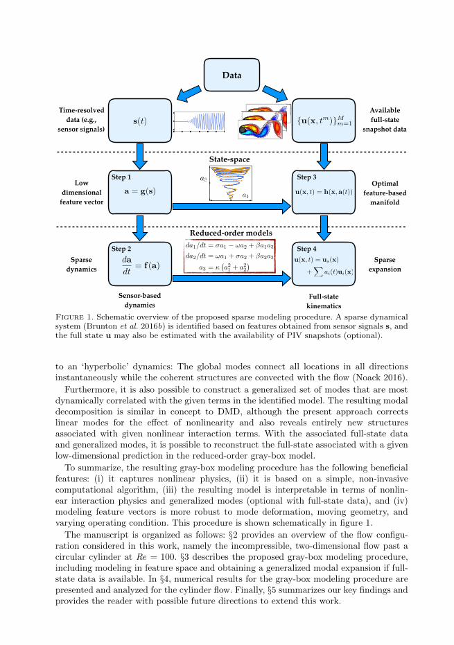
Figure 1. Schematic overview of the proposed sparse modeling procedure. A sparse dynamicalsystem (Brunton et al. 2016b) is identified based on features obtained from sensor signals s, andthe full state u may also be estimated with the availability of PIV snapshots (optional).
to an ‘hyperbolic’ dynamics: The global modes connect all locations in all directionsinstantaneously while the coherent structures are convected with the flow (Noack 2016).
Furthermore, it is also possible to construct a generalized set of modes that are mostdynamically correlated with the given terms in the identified model. The resulting modaldecomposition is similar in concept to DMD, although the present approach correctslinear modes for the effect of nonlinearity and also reveals entirely new structuresassociated with given nonlinear interaction terms. With the associated full-state dataand generalized modes, it is possible to reconstruct the full-state associated with a givenlow-dimensional prediction in the reduced-order gray-box model.
To summarize, the resulting gray-box modeling procedure has the following beneficialfeatures: (i) it captures nonlinear physics, (ii) it is based on a simple, non-invasivecomputational algorithm, (iii) the resulting model is interpretable in terms of nonlin-ear interaction physics and generalized modes (optional with full-state data), and (iv)modeling feature vectors is more robust to mode deformation, moving geometry, andvarying operating condition. This procedure is shown schematically in figure 1.
The manuscript is organized as follows: §2 provides an overview of the flow configu-ration considered in this work, namely the incompressible, two-dimensional flow past acircular cylinder at Re = 100. §3 describes the proposed gray-box modeling procedure,including modeling in feature space and obtaining a generalized modal expansion if full-state data is available. In §4, numerical results for the gray-box modeling procedure arepresented and analyzed for the cylinder flow. Finally, §5 summarizes our key findings andprovides the reader with possible future directions to extend this work.
Sparse reduced-order modeling 5
2. Flow configuration
The flow configuration considered in the present work is the two-dimensional incom-pressible viscous flow past a circular cylinder at Re = 100. This Reynolds number, basedon the free-stream velocity U∞, the cylinder diameter D and the kinematic viscosity ν,is well above the onset of vortex shedding (Zebib 1987; Schumm et al. 1994) and belowthe onset of three-dimensional instabilities (Zhang et al. 1995; Barkley & Henderson1996). In the fluid dynamics community, a large body of literature exists in which thisparticular setup has been chosen to illustrate modal decomposition (Bagheri 2013) andmodel identification techniques (Noack et al. 2003; Sengupta et al. 2015; Brunton et al.2016b; Rowley & Dawson 2016). This setup is thus a particularly compelling test case toillustrate our model identification strategy, as well as to draw connections and quantifyits performance against other well-established techniques.
The dynamics of the flow are governed by the incompressible Navier-Stokes equations
∂u
∂t+ (u · ∇)u = −∇p+
1
Re∇2u
∇ · u = 0,(2.1)
where u = (u, v)T and p are the velocity and pressure fields, respectively. The centerof the cylinder has been chosen as the origin of the reference frame x = (x, y), wherex denotes the streamwise coordinate and y denotes the spanwise coordinate. This studyconsiders the same computational domain as in Noack et al. (2003), extending fromx = −5 to x = 15 in the streamwise direction, and from y = −5 to y = 5 in the spanwisedirection. A uniform velocity profile is prescribed at the inflow, a classical stress-freeboundary condition is used at the outflow, and free-slip boundary conditions are usedon the lateral boundaries of the computational domain. Based on the spectral elementsolver Nek 5000 (Fischer et al. 2008), the domain is discretized by 1832 seventh-orderspectral elements. Finally, the time-integration of the diffusive terms relies on a BackwardDifferentiation of order 3 (BDF3), while the convective terms are advanced in time basedon a third-order accurate extrapolation.
Many of the direct numerical simulations performed in this work have been initializedwith the following initial condition
u(x, 0) = us(x) + 0.001ε(x), (2.2)
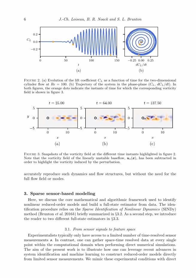
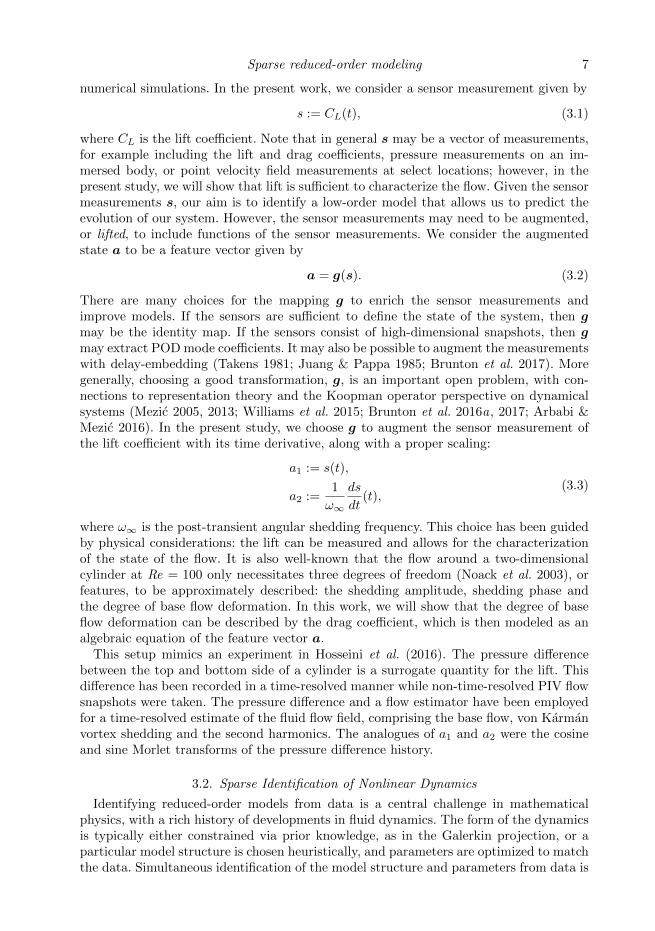
where us(x) is the linearly unstable steady solution of the Navier-Stokes equations andε(x) is a zero-mean and unit-variance random white-noise velocity field. Each simulationis run for 150 convective time units, providing M = 1200 equidistantly sampled velocitysnapshots um(x) = u(x, tm), m = 1, · · · ,M , and associated measurements of the lift anddrag coefficients, CL(tm) and CD(tm). This time-span covers the entire unforced transientphase, from the steady solution to the fully developed von Karman vortex street. Figure2 depicts a typical evolution of the lift coefficient CL, while figure 3 shows snapshotsof the vorticity field at different instants of time. For t 6 50, the flow is governed bylinear dynamics. Consequently, the vorticity field of the perturbation v(x, t) = u(x, t)−us(x), as shown in figure 3(a), can be well approximated by the leading instability mode.For 50 6 t 6 80, the perturbation grows to an extent that nonlinear effects cause theperturbation to distort. Eventually, for t > 80, the flow settles onto a periodic limit cyclecorresponding to the onset of the von Karman vortex street. Given the evolution of thelift coefficient depicted in figure 2 and the associated snapshots shown in figure 3, theaim of the present work is to propose a new reduced-order modeling strategy able to
6 J.-Ch. Loiseau, B. R. Noack and S. L. Brunton
0 50 100 150t
−0.2
0.0
0.2CL
(a)
−0.25 0.00 0.25dCL/dt
(b)
Figure 2. (a) Evolution of the lift coefficient CL as a function of time for the two-dimensionalcylinder flow at Re = 100. (b) Trajectory of the system in the phase-plane (CL, dCL/dt). Inboth figures, the orange dots indicate the instants of time for which the corresponding vorticityfield is shown in figure 3.
Figure 3. Snapshots of the vorticity field at the different time instants highlighted in figure 2.Note that the vorticity field of the linearly unstable baseflow, us(x), has been subtracted inorder to highlight the vorticity induced by the perturbation.
accurately reproduce such dynamics and flow structures, but without the need for thefull flow field or modes.
3. Sparse sensor-based modeling
Here, we discuss the core mathematical and algorithmic framework used to identifynonlinear reduced-order models and build a full-state estimator from data. The iden-tification procedure relies on the Sparse Identification of Nonlinear Dynamics (SINDy)method (Brunton et al. 2016b) briefly summarized in §3.2. As a second step, we introducethe reader to two different full-state estimators in §3.3.
3.1. From sensor signals to feature space
Experimentalists typically only have access to a limited number of time-resolved sensormeasurements s. In contrast, one can gather space-time resolved data at every singlepoint within the computational domain when performing direct numerical simulations.The aim of the present work is to illustrate how one can leverage recent advances insystem identification and machine learning to construct reduced-order models directlyfrom limited sensor measurements. We mimic these experimental conditions with direct
Sparse reduced-order modeling 7
numerical simulations. In the present work, we consider a sensor measurement given by
s := CL(t), (3.1)
where CL is the lift coefficient. Note that in general s may be a vector of measurements,for example including the lift and drag coefficients, pressure measurements on an im-mersed body, or point velocity field measurements at select locations; however, in thepresent study, we will show that lift is sufficient to characterize the flow. Given the sensormeasurements s, our aim is to identify a low-order model that allows us to predict theevolution of our system. However, the sensor measurements may need to be augmented,or lifted, to include functions of the sensor measurements. We consider the augmentedstate a to be a feature vector given by
a = g(s). (3.2)
There are many choices for the mapping g to enrich the sensor measurements andimprove models. If the sensors are sufficient to define the state of the system, then gmay be the identity map. If the sensors consist of high-dimensional snapshots, then gmay extract POD mode coefficients. It may also be possible to augment the measurementswith delay-embedding (Takens 1981; Juang & Pappa 1985; Brunton et al. 2017). Moregenerally, choosing a good transformation, g, is an important open problem, with con-nections to representation theory and the Koopman operator perspective on dynamicalsystems (Mezic 2005, 2013; Williams et al. 2015; Brunton et al. 2016a, 2017; Arbabi &Mezic 2016). In the present study, we choose g to augment the sensor measurement ofthe lift coefficient with its time derivative, along with a proper scaling:
a1 := s(t),
a2 :=1
ω∞
ds
dt(t),
(3.3)
where ω∞ is the post-transient angular shedding frequency. This choice has been guidedby physical considerations: the lift can be measured and allows for the characterizationof the state of the flow. It is also well-known that the flow around a two-dimensionalcylinder at Re = 100 only necessitates three degrees of freedom (Noack et al. 2003), orfeatures, to be approximately described: the shedding amplitude, shedding phase andthe degree of base flow deformation. In this work, we will show that the degree of baseflow deformation can be described by the drag coefficient, which is then modeled as analgebraic equation of the feature vector a.
This setup mimics an experiment in Hosseini et al. (2016). The pressure differencebetween the top and bottom side of a cylinder is a surrogate quantity for the lift. Thisdifference has been recorded in a time-resolved manner while non-time-resolved PIV flowsnapshots were taken. The pressure difference and a flow estimator have been employedfor a time-resolved estimate of the fluid flow field, comprising the base flow, von Karmanvortex shedding and the second harmonics. The analogues of a1 and a2 were the cosineand sine Morlet transforms of the pressure difference history.
3.2. Sparse Identification of Nonlinear Dynamics
Identifying reduced-order models from data is a central challenge in mathematicalphysics, with a rich history of developments in fluid dynamics. The form of the dynamicsis typically either constrained via prior knowledge, as in the Galerkin projection, or aparticular model structure is chosen heuristically, and parameters are optimized to matchthe data. Simultaneous identification of the model structure and parameters from data is
8 J.-Ch. Loiseau, B. R. Noack and S. L. Brunton
considerably more challenging, as there are combinatorially many possible model struc-tures. The sparse identification of nonlinear dynamics (SINDy) architecture (Bruntonet al. 2016b) bypasses the intractable combinatorial search through all possible modelstructures, leveraging the fact that many systems may be modeled by dynamics f thatare sparse in the space of possible right-hand side functions:
da
dt= f(a), (3.4)
where a is the same state vector as in §3.1. It is then possible to solve for the relevantterms that are active in the dynamics using either a convex `1-regularized regression (Tib-shirani 1996) or a sequentially thresholded least-squares (Brunton et al. 2016b); thesealgorithms penalize the number of terms in the dynamics and scale favorably to largeproblems.
First, time-series data is collected and formed into a data matrix:
A =[a(t1) a(t2) · · · a(tM )
]T(3.5)
where ‘T ’ denotes the matrix transpose. A similar matrix of derivatives is formed:
A =
[da
dt(t1)
da
dt(t2) · · · da
dt(tM )
]T. (3.6)
In practice, this may be computed directly from the data in A. However, for noisy data,the total-variation regularized derivative (Chartrand 2011) tends to provide numericallyrobust derivatives. Based on the data in A, a library of candidate nonlinear functionsΘ(A) is constructed:
Θ(A) =[1 A A2 · · · Ad · · · sin(A) · · ·
]. (3.7)
Here, the matrix Ad denotes a matrix with column vectors given by all possible time-series of d-th degree polynomials in the state a. The dynamical system in Eq. (3.4) maynow be represented in terms of the data matrices in Eqs. (3.6) and (3.7) as
A = Θ(A)Ξ. (3.8)
Each column Ξk in Ξ is a vector of coefficients determining the active terms in the k-throw equation in Eq. (3.4). A parsimonious model will provide an accurate model fit inEq. (3.8) with as few terms as possible in Ξ. Such a model may be identified using aconvex `1-regularized sparse regression:
Ξk = argminΞ′
k
‖Ak −Θ(A)Ξ′k‖2 + λ‖Ξ′k‖1. (3.9)
Here, Ak is the k-th column of A. Sparse regression, such as the LASSO (Tibshirani1996) or the sequential thresholded least-squares algorithm used in SINDy, improvesthe numerical robustness of this identification for noisy overdetermined problems, incontrast to earlier methods (Wang et al. 2011) that used compressed sensing (Donoho2006; Candes 2006). Once identified, the sparse vectors Ξk may be synthesized into anonlinear dynamical system model:
dakdt
= Θ(a)Ξk, (3.10)
where ak is the k-th element of a and Θ(a) is a row vector of symbolic functions ofa, as opposed to the data matrix Θ(A). Identifying the most parsimonious nonlinearmodel by applying sparse regression in the library Θ is a convex procedure. The
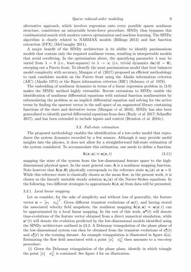
Sparse reduced-order modeling 9
alternative approach, which involves regression onto every possible sparse nonlinearstructure, constitutes an intractable brute-force procedure. SINDy thus bypasses thiscombinatorial search with modern convex optimization and machine learning. The SINDyalgorithm is closely related to NARMAX models (Billings 2013) and fast functionextraction (FFX) (McConaghy 2011).
A major benefit of the SINDy architecture is its ability to identify parsimoniousmodels that contain only the required nonlinear terms, resulting in interpretable modelsthat avoid overfitting. In the optimization above, the sparsifying parameter λ may bevaried from λ = 0 (i.e., least-squares) to λ → ∞ (i.e, trivial dynamics da/dt = 0),sweeping out a Pareto front. To identify the most parsimonious model that best balancesmodel complexity with accuracy, Mangan et al. (2017) proposed an efficient methodologyto rank candidate models on the Pareto front using the Akaike information criterion(AIC) (Akaike 1974) or the Bayes information criterion (BIC) (Schwarz et al. 1978).
The embedding of nonlinear dynamics in terms of a linear regression problem in (3.9)makes the SINDy method highly extensible. Recent extensions to SINDy enable theidentification of nonlinear differential equations with rational function nonlinearities byreformulating the problem as an implicit differential equation and solving for the activeterms by finding the sparsest vector in the null space of an augmented library containingfunctions of the state and derivative terms (Mangan et al. 2016). SINDy has also beengeneralized to identify partial differential equations from data (Rudy et al. 2017; Schaeffer2017), and has been extended to include inputs and control (Brunton et al. 2016c).
3.3. Full-state estimation
The proposed methodology enables the identification of a low-order model that repro-duces the system dynamics recorded by a few sensors. Although it may provide usefulinsights into the physics, it does not allow for a straightforward full-state estimation ofthe system considered. To accommodate this estimation, one needs to define a function
h(x,a) ≈ u(x, t) (3.11)
mapping the state of the system from the low-dimensional feature space to the high-dimensional physical space. In the most general case, h is a nonlinear mapping function.Note however that h(x,0) physically corresponds to the reference state us(x) at a = 0.While this reference state is classically chosen as the mean flow, in the present work, it ischosen as the linearly unstable steady solution us(x) of the Navier-Stokes equations. Inthe following, two different strategies to approximate h(x,a) from data will be presented.
3.3.1. Local linear mapping
Let us consider, for the sake of simplicity and without loss of generality, the feature
vector a =[a1 a2
]T. Given different transient evolutions of a(t), and having stored
the associated velocity field snapshots, the nonlinear mapping h(x,a) ≈ u(x, t) canbe approximated by a local linear mapping. In the rest of this work, a•(t) will denotetime-evolutions of the feature vector obtained from a direct numerical simulation, whilea◦(t) will denote the evolution predicted by the low-dimensional models identified usingthe SINDy architecture outlined in §3.2. A Delaunay triangulation of the phase plane ofthe low-dimensional system can then be obtained from the transient evolutions of a•1(t)and a•2(t) in the training dataset. An example triangulation is illustrated in figure 4(a).Estimating the flow field associated with a point
[a◦1 a◦2
]then amounts to a two-step
procedure:(i) Given the Delaunay triangulation of the phase plane, identify in which triangle
the point[a◦1 a◦2
]is contained. See figure 4 for an illustration.
10 J.-Ch. Loiseau, B. R. Noack and S. L. Brunton
−1.5 0.0 1.5a1
−1.5
0.0
1.5
a2
(a)
−0.6 −0.5 −0.4a1
0.0
0.1
0.2
a2
(b)
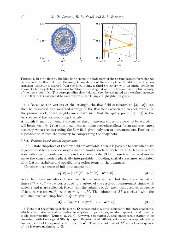
Figure 4. In both figures, the blue line depicts the trajectory of the testing dataset for which wereconstruct the flow field. (a) Delaunay triangulation of the state plane. In addition to the twotransient trajectories started from the fixed point, a third trajectory with an initial conditionabove the limit cycle has been used to obtain this triangulation. (b) Close-up view in the vicinityof the query point (•). The corresponding flow field can then be estimated as a weighted averageof the flow fields associated to each vertex of the triangle highlighted in green.
(ii) Based on the vertices of this triangle, the flow field associated to[a◦1 a◦2
]can
then be estimated as a weighted average of the flow fields associated to each vertex. Inthe present work, these weights are chosen such that the query point
[a◦1 a◦2
]is the
barycentre of the corresponding triangle.Although it may be memory–intensive, since numerous snapshots need to be stored, itwill be shown in §4.2 that this local linear mapping procedure allows for an unprecedentedaccuracy when reconstructing the flow field given only sensor measurements. Further, itis possible to reduce the memory by compressing the snapshots.
3.3.2. Feature-based modal expansion
If full-state snapshots of the flow field are available, then it is possible to construct a setof generalized feature-based modes that are most correlated with either the feature vectora or with specific nonlinear terms in the sparse model (3.4). These feature-based modesmake the sparse models physically interpretable, providing spatial structures associatedwith feature variables and specific interaction terms in the dynamics.
Consider a sequence of full-state snapshots‡Q(x) =
[um1(x) um2(x) ump(x)
]. (3.12)
Note that these snapshots do not need to be time-resolved, but they are collected attimes tm1 , · · · , tmp that correspond to a subset of the resolved measurement times withwhich s and a are collected. Recall that the columns of AT are a time-resolved sequenceof feature vectors a(tm), with m = 1, · · · ,M . The columns of AT associated with thenon-time-resolved snapshots in Q are given by
ATQ =
[a(tm1) a(tm2) · · · a(tmp)
]. (3.13)
‡ Note that the columns of the matrix Q correspond to a time-sequence of full-state snapshots,which is the mathematical convention in snapshot proper orthogonal decomposition and dynamicmode decomposition (Kutz et al. 2016). However, the matrix A uses transposed notation to beconsistent with the original SINDy paper (Brunton et al. 2016b), with rows corresponding to atime-sequence of transposed feature vectors aT . Thus, the columns of AT are a time-sequenceof the features a, similar to Q.
Sparse reduced-order modeling 11
Thus, the snapshots sequence may be approximated by
Q = U(x)ATQ(t) +R(x, t), (3.14)
where R is the truncation residual. The columns of U(x) are feature-based modes thatare most correlated with the terms in the feature vector a(t). These modes are found vialeast-squares regression:
U = Q(ATQ
)†, (3.15)
where(ATQ
)†is the Moore-Penrose pseudo-inverse of AT
Q. In practice, this least-squares
regression may be solved efficiently using the singular value decomposition of ATQ.
More generally, it is possible to compute modes that are most correlated with thedynamic interaction terms in the sparse model (3.8). Let γ1, · · · , γq denote the indicesof the rows in Ξ with non-zero entries, i.e. corresponding to active terms in the sparsedynamics. The corresponding terms in the dynamics may be extracted via:
α =(Θ(a)
[eγ1 eγ2 · · · eγq
])T, (3.16)
where eγj is a column vector consisting entirely of zeros, except for a one in the γj-th row;i.e., eγj is the γj-th column of the identity matrix. For example, in the results, we will con-
sider a vector of nonlinear terms α given by α =[a1 a2 a21 + a22 2a1a2 a21 − a22
]T.
It is now possible to obtain generalized modes:
U = Q([α(tm1) α(tm2) · · · α(tmp)
])†. (3.17)
Thus, each mode ui(x) is a spatial field corresponding to a specific interaction term inthe dynamical system, given by a component of α.
Compared to the local linear mapping presented in §3.3.1, such a feature-based expan-sion has a low memory footprint, although it will typically be less accurate. However,even if the feature-based modes are not used for full-state reconstruction, they imbuethe sparse model with physical interpretability. The modal representation above may bethought of as closely related to the proper orthogonal decomposition or dynamic modedecomposition, except generalized to identify modes that are most correlated with thefeatures in a or the dynamic interaction terms in α.
4. Results
4.1. Sensor-based dynamics
In this section, a low-dimensional model of the transient and post-transient laminarcylinder wake is presented. First, a dynamical model capturing the dynamics of the liftcoefficient is identified in §4.1.1. Then, in §4.1.2, the low-order model aforementionedis supplemented with a nonlinear algebraic measurement equation in order to infer theevolution of the drag coefficient.
4.1.1. Dynamical system
It is well known that the two-dimensional cylinder flow behaves as a self-excited, self-limiting and nearly harmonic nonlinear oscillator. This behavior is clearly visible in thetime-evolution of the instantaneous lift coefficient depicted in figure 2. As such, thedynamics can be described by a nonlinear second-order ordinary differential equation, orby a set of two coupled first-order ODEs. Given our feature vector a (3.3), mapping thestate of the system from the sensor-space to the feature-space, is defined as
a =[a1 a2
]T, (4.1)
12 J.-Ch. Loiseau, B. R. Noack and S. L. Brunton
with a =a
amax, amax being the maximum value of a once the system evolves onto the
periodic limit cycle. Such normalization ensures that
−1 6 a1,2 6 1,
a condition which greatly simplifies the sparse optimization problem involved in theidentification procedure. Although this mapping function has been defined analyticallyin the present work, similar features could be identified using delay coordinates, as in thesingular spectrum analysis (SSA) in meteorology and ecology (Colebrook 1978; Barnett &Hasselmann 1979; Weare & Nasstrom 1982; Ghil et al. 2002), NARMAX (Billings 2013),the eigensystem realization algorithm (ERA) from system identification and controltheory (Juang & Pappa 1985); these delay coordinates have recently been connectedto the linear embedding of nonlinear dynamics via Koopman operator theory (Bruntonet al. 2017; Arbabi & Mezic 2016). Alternatively, one could have also used the Hilberttransform for that purpose.
Based on the different transient time evolutions of s•(t) recorded from direct numericalsimulations, the corresponding feature vectors a•(t) have been computed and groupedinto our training dataset. The Sparse Identification of Nonlinear Dynamics (Bruntonet al. 2016b), briefly outlined in §3.2, is used to identify the equations governing thedynamics of a. The pool of candidate functions required for the identification process ischosen as
Θ(a1, a2) =[1 a1 a2 a21 a1a2 a22 a31 a21a2 a1a
22 a32
]. (4.2)
Such a pool of polynomial functions, which can easily be enriched if needed, is a naturalchoice for the identification of a nonlinear oscillator (Holmes & Guckenheimer 1983). Inthe present case, it leads to the identification of the following dynamical system
d
dt
[a1a2
]=
[0 1.12
−1.116 0.28(1− a21 − a22)
] [a1a2
]. (4.3)
More details about the model selection procedure can be found in appendix A. As shownin figure 5, the time evolution of a◦1(t) predicted by this low-dimensional system is in verygood agreement with the one obtained for a•1(t) based on a direct numerical simulationwhose initial condition has been chosen in the vicinity of the linearly unstable baseflow.It is also remarkable that, despite its apparent simplicity, this two-degrees-of-freedomsystem captures all of the key physics of the cylinder flow, namely:• It admits only one linearly unstable fixed point given by a = 0 and one attracting
limit cycle characterized by ‖a‖ = 1. The corresponding circular frequency ω◦ = 1.119 inthe nonlinearly saturated state is moreover less than 1.5% smaller than the one observedin DNS (ω• = 1.132).• It explicitly highlights the quadratic dependency of the instantaneous growth rate
2σ(a) = 0.28(1 − a21 − a22). Such quadratic dependencies are in line with our currentunderstanding of the nonlinear saturation process of globally unstable flows; see Mantic-Lugo et al. (2014) for more details.• Once the amplitude of the oscillation has saturated to ‖a‖ = 1, the system reduces
to a simple harmonic oscillator. A similar structure could be derived based on a Galerkinprojection of the Navier-Stokes equations onto the span of the first two POD modes andusing the marginally stable mean flow as the reference state.From a physical point of view, this low-order system describes the dynamics of the originalhigh-dimensional system when constrained to the low-dimensional manifold structuringits phase phase (Noack et al. 2003).
Sparse reduced-order modeling 13
0 50 100 150t
−1
0
1
a1
(a)
Raw data a•(t) Model a◦(t)
−1 0 1a2
(b)
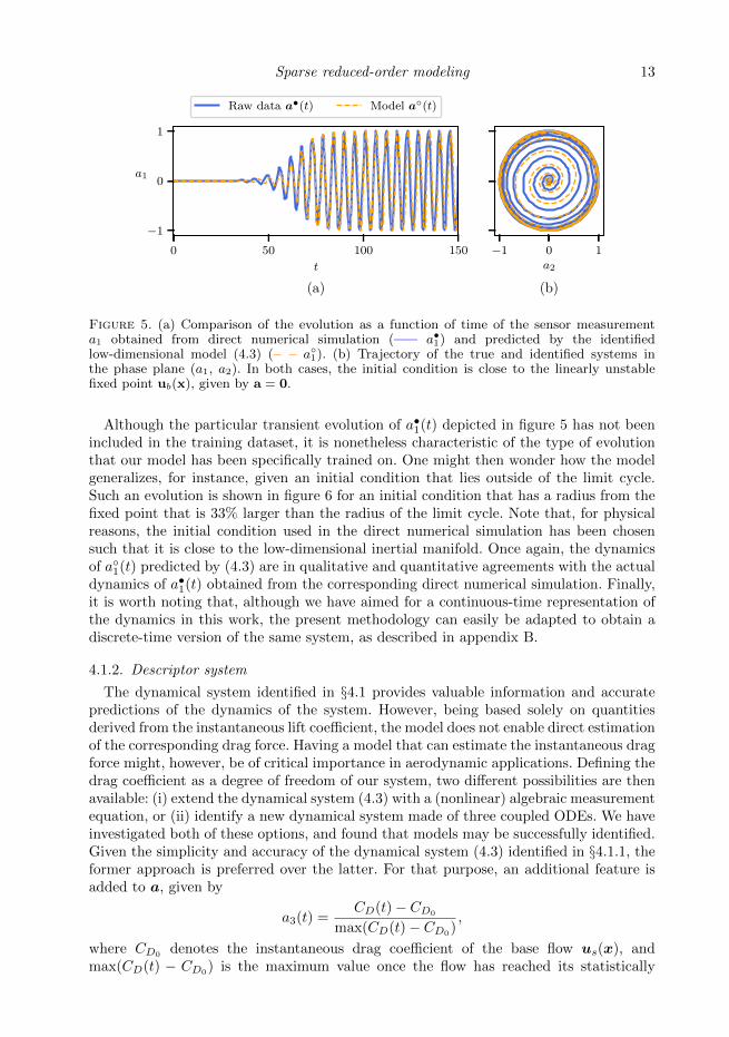
Figure 5. (a) Comparison of the evolution as a function of time of the sensor measurementa1 obtained from direct numerical simulation (—– a•1) and predicted by the identifiedlow-dimensional model (4.3) (– – a◦1). (b) Trajectory of the true and identified systems inthe phase plane (a1, a2). In both cases, the initial condition is close to the linearly unstablefixed point ub(x), given by a = 0.
Although the particular transient evolution of a•1(t) depicted in figure 5 has not beenincluded in the training dataset, it is nonetheless characteristic of the type of evolutionthat our model has been specifically trained on. One might then wonder how the modelgeneralizes, for instance, given an initial condition that lies outside of the limit cycle.Such an evolution is shown in figure 6 for an initial condition that has a radius from thefixed point that is 33% larger than the radius of the limit cycle. Note that, for physicalreasons, the initial condition used in the direct numerical simulation has been chosensuch that it is close to the low-dimensional inertial manifold. Once again, the dynamicsof a◦1(t) predicted by (4.3) are in qualitative and quantitative agreements with the actualdynamics of a•1(t) obtained from the corresponding direct numerical simulation. Finally,it is worth noting that, although we have aimed for a continuous-time representation ofthe dynamics in this work, the present methodology can easily be adapted to obtain adiscrete-time version of the same system, as described in appendix B.
4.1.2. Descriptor system
The dynamical system identified in §4.1 provides valuable information and accuratepredictions of the dynamics of the system. However, being based solely on quantitiesderived from the instantaneous lift coefficient, the model does not enable direct estimationof the corresponding drag force. Having a model that can estimate the instantaneous dragforce might, however, be of critical importance in aerodynamic applications. Defining thedrag coefficient as a degree of freedom of our system, two different possibilities are thenavailable: (i) extend the dynamical system (4.3) with a (nonlinear) algebraic measurementequation, or (ii) identify a new dynamical system made of three coupled ODEs. We haveinvestigated both of these options, and found that models may be successfully identified.Given the simplicity and accuracy of the dynamical system (4.3) identified in §4.1.1, theformer approach is preferred over the latter. For that purpose, an additional feature isadded to a, given by
a3(t) =CD(t)− CD0
max(CD(t)− CD0),
where CD0 denotes the instantaneous drag coefficient of the base flow us(x), andmax(CD(t) − CD0) is the maximum value once the flow has reached its statistically
14 J.-Ch. Loiseau, B. R. Noack and S. L. Brunton
0 10 20 30 40 50t
−1
0
1
a1
(a)
Raw data a•(t) Model a◦(t)
−1 0 1a2
(b)
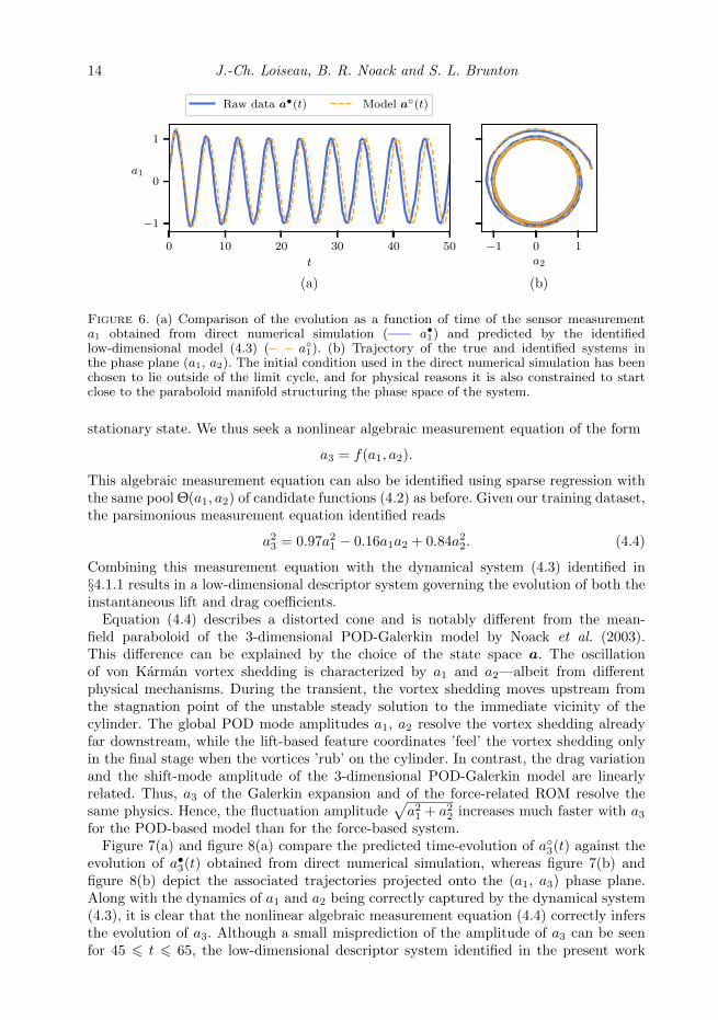
Figure 6. (a) Comparison of the evolution as a function of time of the sensor measurementa1 obtained from direct numerical simulation (—– a•1) and predicted by the identifiedlow-dimensional model (4.3) (– – a◦1). (b) Trajectory of the true and identified systems inthe phase plane (a1, a2). The initial condition used in the direct numerical simulation has beenchosen to lie outside of the limit cycle, and for physical reasons it is also constrained to startclose to the paraboloid manifold structuring the phase space of the system.
stationary state. We thus seek a nonlinear algebraic measurement equation of the form
a3 = f(a1, a2).
This algebraic measurement equation can also be identified using sparse regression withthe same pool Θ(a1, a2) of candidate functions (4.2) as before. Given our training dataset,the parsimonious measurement equation identified reads
a23 = 0.97a21 − 0.16a1a2 + 0.84a22. (4.4)
Combining this measurement equation with the dynamical system (4.3) identified in§4.1.1 results in a low-dimensional descriptor system governing the evolution of both theinstantaneous lift and drag coefficients.
Equation (4.4) describes a distorted cone and is notably different from the mean-field paraboloid of the 3-dimensional POD-Galerkin model by Noack et al. (2003).This difference can be explained by the choice of the state space a. The oscillationof von Karman vortex shedding is characterized by a1 and a2—albeit from differentphysical mechanisms. During the transient, the vortex shedding moves upstream fromthe stagnation point of the unstable steady solution to the immediate vicinity of thecylinder. The global POD mode amplitudes a1, a2 resolve the vortex shedding alreadyfar downstream, while the lift-based feature coordinates ’feel’ the vortex shedding onlyin the final stage when the vortices ’rub’ on the cylinder. In contrast, the drag variationand the shift-mode amplitude of the 3-dimensional POD-Galerkin model are linearlyrelated. Thus, a3 of the Galerkin expansion and of the force-related ROM resolve thesame physics. Hence, the fluctuation amplitude
√a21 + a22 increases much faster with a3
for the POD-based model than for the force-based system.Figure 7(a) and figure 8(a) compare the predicted time-evolution of a◦3(t) against the
evolution of a•3(t) obtained from direct numerical simulation, whereas figure 7(b) andfigure 8(b) depict the associated trajectories projected onto the (a1, a3) phase plane.Along with the dynamics of a1 and a2 being correctly captured by the dynamical system(4.3), it is clear that the nonlinear algebraic measurement equation (4.4) correctly infersthe evolution of a3. Although a small misprediction of the amplitude of a3 can be seenfor 45 6 t 6 65, the low-dimensional descriptor system identified in the present work

Sparse reduced-order modeling 15
0 20 40 60 80 100 120 140t
0.0
0.5
1.0a
3
(a)
Raw data Descriptor System
−1 0 1a1
(b)
Figure 7. (a) Comparison of the evolution as a function of time of the sensor measurementa3 obtained from direct numerical simulation (—– a•3) and predicted by the identifiedlow-dimensional descriptor system made of (4.3) and (4.4) (– – a◦3). (b) Trajectory of thetrue system and the identified one in the phase plane (a1, a3).
0 10 20 30 40 50t
0.9
1.0
1.1
1.2
a3
(a)
Raw data Descriptor System
−1 0 1a1
(b)
Figure 8. (a) Comparison of the evolution as a function of time of the sensor measurementa3 obtained from direct numerical simulation (—– a•3) and predicted by the identifiedlow-dimensional descriptor system made of (4.3) and (4.4) (– – a◦3). (b) Trajectory of thetrue system and the identified one in the phase plane (a1, a3).
is nonetheless one of the simplest and yet most accurate and physically interpretablelow-order models available in the literature to reproduce the dynamics of the cylinderflow at Re = 100.
4.2. Flow field estimation
The descriptor system identified in the previous section provides valuable informationand accurate predictions of the dynamics of the system. However, it does not allow us todirectly infer what the corresponding flow field is. In order to estimate the flow, we thusneed to supplement our dynamical system with a full-state estimator given by
u(x, t) ≈ h(x,a(t)).
Formally, this full-state estimator h is a nonlinear mapping from the low-dimensionalfeature-space to the high-dimensional physical space. In the rest of this section, twodifferent strategies will be employed in order to build this nonlinear mapping: the local

16 J.-Ch. Loiseau, B. R. Noack and S. L. Brunton
linear mapping procedure described in §3.3, or a feature-based modal expansion of thevelocity field in terms of the feature modes introduced in §3.3.2.
Given a sparse nonlinear model, it is also possible to construct a generalized feature-based modal decomposition that identifies modal structures that are most correlatedwith specific terms in the dynamics. We define a new feature vector α containing all ofthe nonzero terms identified in the right hand side of the sparse model:
α ,
a1a2
a21 + a222a1a2a21 − a22
=
α1
α2
α3
α4
α5
. (4.5)
The feature-based modal expansion considered hereafter then reads
u(x, t) = u0(x) +
5∑
i=1
ui(x)αi(t) + r(x, t) (4.6)
where u0(x) is the linearly unstable steady solution to the Navier-Stokes equations andr(x, t) the residual. The different feature modes ui(x) have been computed followingthe procedure described in §3.3. Mathematically, the generalized mode decomposition isachieved with a simple least-squares regression:
Q ≈
u1(x) u2(x) u3(x) u4(x) u5(x)
︸ ︷︷ ︸Modes: U
α1(t)α2(t)α3(t)α4(t)α5(t)
︸ ︷︷ ︸Time dynamics: α(t)
=⇒ U = Q (α(t))†
(4.7)
where (α(t))†
denotes the pseudo-inverse of the matrix α(t), and Q is the sequence ofbaseflow-substracted snapshots.
The associated vorticity fields are shown in figure 10, while the time-evolution of thedifferent basis coefficients αi(t) is depicted in figure 9(a). Figure 9(b) shows the crosscorrelation matrix of these signals. Given its diagonal structure, it is clear that thedifferent basis coefficients αi(t) are uncorrelated one to another. For the cylinder flow,these feature modes are very similar to the classical POD modes. A key advantage overPOD modes is that the present modes are directly interpretable as being the coherentstructures most correlated with our different measurements and the sparse nonlinearinteraction terms in the model. Moreover, the shift mode u3 naturally arises in thisframework as the result of quadratic interactions between a1 and a2, consistent with ourunderstanding of the nonlinear saturation of globally unstable flows (Mantic-Lugo et al.2014). Defining the feature vector α used in the feature-based modal expansion suchthat it includes quadratic terms was thus deemed necessary in order to ensure that thedistortion between the linearly unstable base flow and the marginally stable mean flow iscorrectly captured by the flow estimator using the feature-based modal expansion (4.6).
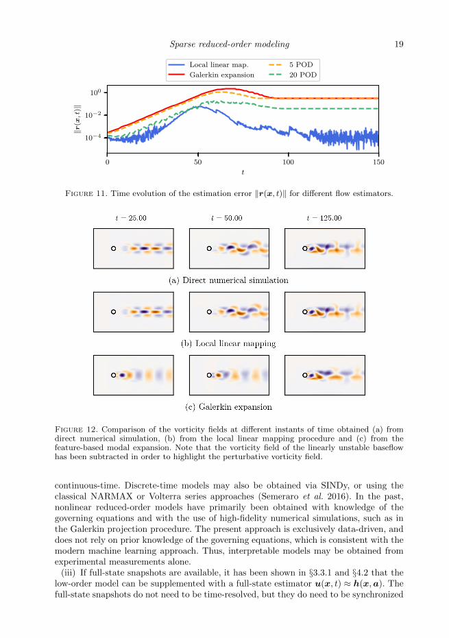
Figure 11 compares the evolution of ‖r‖, i.e. the norm of the estimation error, for thelocal linear mapping and the feature-based modal expansion (4.6). The evolution of thetruncation error for different POD bases is also reported for the sake of comparison. Theflow estimator based on the local linear mapping (LLM) largely outperforms the twoestimators based on a 5-mode POD expansion and the generalized modal decomposition

Sparse reduced-order modeling 17
with 5 modes. Its very good performances, on average two to three orders of magnitudemore accurate than the other estimators considered, results from the fact that LLMleverages all of the information contained in the different snapshots matrices used whereasthe different modal expansions only provide low-rank approximations of these samematrices. However, this higher accuracy comes at the price of increased storage. Thisrequirement can nonetheless be mitigated by computing a low-rank approximation ofthe snapshot matrix used in the training dataset. In the present case, considering a rank-50 approximation based on the singular value decomposition has almost no effect on theestimation error, while significantly reducing the memory requirements. Instead of storingM = 1, 200 snapshots, each a 100,000-dimensional vector corresponding to a vertex ofthe Delaunay triangulation of phase space, only the 50 leading full-state singular vectorsmust be stored, along with the 50-dimensional vector of coefficients for each vertex. Thisreduces the storage requirements by a factor of nearly 24. In this case, the local linearmapping would then approximate the transfer function mapping the state of our systemfrom the 2-dimensional phase space of the dynamical system (4.3) to the 50-dimensionalspace of coefficients resulting from the truncated singular value decomposition of thesnapshots matrix.
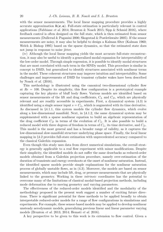
Finally, figures 12(b) and (c) depict the estimated vorticity field, with the base flowsubtracted, at different instants in time and compare them with the true vorticity fieldobtained from direct numerical simulation in figure 12(a). The vorticity fields estimatedusing the local linear mapping are in much better agreement, from a physical andkinematic point of view, than the ones obtained by the 5-mode modal expansion. This isespecially pronounced during the period of exponential growth of the linear instabilityand at the onset of nonlinear saturation during which the local linear mapping correctlycaptures the deformation and distortion of the flow structure. In contrast, low-rank modalexpansions are notorious for their inability to capture such mode deformation and/orchanges in operating conditions. Given that the POD modes and generalized featuremodes used in this work essentially approximate the flow structure once the systemhas reached the periodic limit cycle, it is thus expected that they provide only a verycrude estimation of the flow structures when the system evolves in the vicinity of thelinearly unstable base flow. This inability of a modal expansion to easily address modedeformation is one of its key limitations and is the principal reason why the local linearmapping strategy should be preferred. Combining the descriptor system identified in §4.1with the local linear flow estimator finally allows us to construct a two-degrees-of-freedomreduced-order model of the cylinder flow, having an unprecedented accuracy.
5. Conclusions
This work develops a new reduced-order modeling procedure for unsteady fluid flowsthat yields accurate nonlinear models and insight into relevant flow structures. Thisprocedure identifies sparse nonlinear models, not on the full fluid state, but from time-resolved sensor measurements that may be realistically obtained in experiments. Thesparsity of the model prevents overfitting and uncovers key nonlinear interaction terms.If PIV snapshots are also available, not necessarily time-resolved, it is possible toestimate the full-state from the sparse model using local linear mapping: the full-stateis interpolated between the most similar historical flow fields, based on the dynamics. Itis also possible to construct a generalized modal decomposition that identifies coherentstructures most correlated with each interaction term in the sparse nonlinear model.
Our methodology, summarized in figure 1, can be divided into four steps:(i) Given a set of physically relevant sensor measurements s, create a low-dimensional

18 J.-Ch. Loiseau, B. R. Noack and S. L. Brunton
−101
α1
−101
α2
−101
α3
−101
α4
0 50 100 150t
−101
α5
(a)
α1 α2 α3 α4 α5
(b)
Figure 9. (a) Time evolution of the different basis coefficients used in the feature-based modalexpansion (4.6). (b) Corresponding cross-correlation matrix. Dark squares indicate that αi andαj are strongly correlated, while white squares indicate they are uncorrelated.
Figure 10. Figure (a) depicts the vorticity field of the linearly unstable base flow, while thedashed line highlights the spatial extent of the reversed flow region. Figurs (b) to (e) show thevorticity field of the feature modes associated to the feature vector b.
feature vector a that allows for a complete dynamics characterization of the state of thesystem. Although we have used an analytical mapping a = g(s) in the present work, thisprocedure could also be performed, for instance, by means of kernel PCA (Scholkopf et al.1998). Moreover, the sensors could come from force measurements, as in the present work,or from any other time resolved sensor measurements, such as pressure along the body. Inthe case of limited measurements, it may also be possible to augment the state using delaycoordinates (Takens 1981), in the spirit of SSA (Colebrook 1978; Barnett & Hasselmann1979), NARMAX (Billings 2013), ERA (Juang & Pappa 1985), or HAVOK (Bruntonet al. 2017) models; delay coordinates have since been connected to Koopman operatortheory (Brunton et al. 2017; Arbabi & Mezic 2016).
(ii) The second step identifies the equations governing the dynamics of a. In thisstudy, the SINDy algorithm (Brunton et al. 2016b) yields a sparse nonlinear model in
Sparse reduced-order modeling 19
0 50 100 150t
10−4
10−2
100
‖r(x,t
)‖Local linear map.Galerkin expansion
5 POD20 POD
Figure 11. Time evolution of the estimation error ‖r(x, t)‖ for different flow estimators.
Figure 12. Comparison of the vorticity fields at different instants of time obtained (a) fromdirect numerical simulation, (b) from the local linear mapping procedure and (c) from thefeature-based modal expansion. Note that the vorticity field of the linearly unstable baseflowhas been subtracted in order to highlight the perturbative vorticity field.
continuous-time. Discrete-time models may also be obtained via SINDy, or using theclassical NARMAX or Volterra series approaches (Semeraro et al. 2016). In the past,nonlinear reduced-order models have primarily been obtained with knowledge of thegoverning equations and with the use of high-fidelity numerical simulations, such as inthe Galerkin projection procedure. The present approach is exclusively data-driven, anddoes not rely on prior knowledge of the governing equations, which is consistent with themodern machine learning approach. Thus, interpretable models may be obtained fromexperimental measurements alone.
(iii) If full-state snapshots are available, it has been shown in §3.3.1 and §4.2 that thelow-order model can be supplemented with a full-state estimator u(x, t) ≈ h(x,a). Thefull-state snapshots do not need to be time-resolved, but they do need to be synchronized
20 J.-Ch. Loiseau, B. R. Noack and S. L. Brunton
with the sensor measurements. The local linear mapping procedure provides a highlyaccurate approximation h(x,a). Full-state estimation is particularly relevant in controlapplications (Fabbiane et al. 2014; Brunton & Noack 2015; Sipp & Schmid 2016), wherefeedback control is often designed on the full state, which is then estimated from sensormeasurements (Dullerud & Paganini 2000; Skogestad & Postlethwaite 2005). If the sensormeasurements are noisy, it may also be helpful to design a Kalman filter (Kalman 1960;Welch & Bishop 1995) based on the sparse dynamics, so that the estimated state doesnot jump in response to noise jitter.
(iv) Although the local linear mapping yields the most accurate full-state reconstruc-tion, it may also be useful to identify a generalized modal expansion for interpretability ofthe low-order model. Through simple regression, it is possible to identify modal structuresthat are most correlated with each term in the SINDy model. This procedure is similar inconcept to DMD, but generalized to identify structures associated with nonlinear termsin the model. These coherent structures may improve intuition and interpretability. Somechallenges and improvements of DMD for transient cylinder wakes have been describedby Noack et al. (2016).
This methodology is illustrated using the canonical two-dimensional cylinder flowat Re = 100. Despite its simplicity, this flow configuration is a prototypical examplecapturing the key physics of bluff body flows. Various models are identified based onsensor measurements of the lift and drag coefficients, CL and CD, which are physicallyrelevant and are readily accessible in experiments. First, a dynamical system (4.3) isidentified using a single sensor input s = CL, which is augmented with its time derivative.As discussed in §4.1.1, this system models the cylinder flow dynamics, which evolvealong a low-dimensional manifold. Next, in §4.1.2, the same dynamical system may besupplemented with a sparse nonlinear equation to build an algebraic representation ofthe drag coefficient CD in terms of the evolution of CL. It is also possible to build areduced model with three degrees of freedom in terms of CL, its time derivative, and CD.This model is the most general and has a broader range of validity, as it captures thelow-dimensional slow-manifold structure underlying phase space. Finally, the local linearmapping in §4.2 provides full-state estimation with unprecedented accuracy compared tothe classical Galerkin expansion.
Even though this study uses data from direct numerical simulations, the overall strat-egy is generally applicable to a real flow experiment with minor modifications. Despitetheir simplicity, the identified models do not suffer the same drawbacks as reduced-ordermodels obtained from a Galerkin projection procedure, namely over-estimation of theduration of transients and energy overshoots at the onset of nonlinear saturation. Instead,the identified sparse models provide simple explanations for the nonlinear saturationprocess of globally unstable flows, as in (4.3). Moreover, the models are based on sensormeasurements, which may include lift, drag, or pressure measurements that are physicallylinked to the geometry. Working in these intrinsic coordinates has the potential toovercome many of the limitations of classical modal-based projection methods, includingmode deformation due to moving geometry and varying parameters.
The effectiveness of the reduced-order models identified and the modularity of themethodology proposed in the present work suggest a number of exciting future direc-tions. There is significant potential for these methods to be applied broadly to obtaininterpretable reduced-order models for a range of flow configurations in simulations andexperiments. For example, these sensor-based models may be applied to develop nonlinearunsteady aerodynamic models, generalizing previous linear and linear parameter varyingmodels (Brunton et al. 2013, 2014; Hemati et al. 2016).
A key perspective to be given to this work is its extension to flow control. Given a
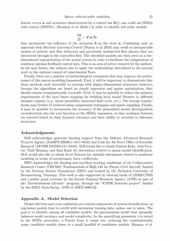
Sparse reduced-order modeling 21
feature vector a and actuators characterized by a control law b(t), one could use SINDywith control (SINDYc) (Brunton et al. 2016c) in order to identify low-order models
da
dt= f(a, b)
that incorporate the influence of the actuation b on the state a. Combining such anapproach with Machine Learning Control (Duriez et al. 2016) may result in interpretablemodels of entirely new flow behaviors and previously unobserved flow physics that arediscovered through in the controlled flow. The identified models can then serve as a low-dimensional representation of the actual system in order to facilitate the computation ofnonlinear optimal feedback control laws. This is an area of active research by the authors.In the near future, the authors aim to apply the methodology introduced in the presentwork to the optimal control of experimental flows.
Finally, there are a number of methodological extensions that may improve the perfor-mance of this sparse modeling framework. First, it will be important to demonstrate thatthese methods scale favorably to systems with higher-dimensional attractors; however,because the algorithms are based on simple regression and sparse optimization, theyshould remain computationally tractable. Next, it may be possible to reduce the memoryrequirements of the local linear mapping by building local modal libraries in differentdynamic regimes (e.g., linear instability, saturated limit cycle, etc.). The storage require-ments may further be reduced using compression techniques and sparse sampling. Finally,it may be possible to incorporate the accuracy of the generalized modal decompositionreconstruction into the cost function in the SINDy regression, so that nonlinear featuresare selected based on their dynamic relevance and their ability to correlate to full-statestructures.
Acknowledgments
SLB acknowledges generous funding support from the Defense Advanced ResearchProjects Agency (DARPA HR0011-16-C-0016) and from the Air Force Office of ScientificResearch (AFOSR FA9550-13-1-0183). SLB would like to thank Nathan Kutz, Josh Proc-tor, Niall Mangan, and Sam Rudy for discussions related to sparse model identification.SLB would also like to thank Scott Dawson for valuable discussions related to nonlinearmodeling in terms of aerodynamic force coefficients.
BRN acknowledges the funding and excellent working conditions of the CollaborativeResearch Center (CRC880) ’Fundamentals of High Lift for Future Civil Aircraft’ fundedby the German Science Foundation (DFG) and hosted by the Technical University ofBraunschweig, Germany. This work is also supported by internal funds of LIMSI-CNRSand a public grant overseen by the French National Research Agency (ANR) as part ofthe “Investissement dAvenir” program, through the “iCODE Institute project” fundedby the IDEX Paris-Saclay, ANR-11-IDEX-0003-02.
Appendix A. Model Selection
Model selection and cross-validation are crucial components of system identification, asregression models tend to overfit with increasing training data, unless care is taken. Thegoal is to identify, among all candidate models, the parsimonious model that optimallybalances model accuracy and model complexity. As the sparsifying parameter λ is variedin the SINDy procedure, a Pareto front is swept out, reducing the combinatoriallymany candidate models down to a small handful of candidates models. Mangan et al.
22 J.-Ch. Loiseau, B. R. Noack and S. L. Brunton
(2017) have recently demonstrated how SINDy can be combined with the well-knownAkaike information criterion (AIC) (Akaike 1974) or the Bayes information criterion(BIC) (Schwarz et al. 1978) in order to select the most parsimonious model from thisPareto front. Given a candidate model, the associated AIC score is given by
AIC = 2k − 2 ln(L(a, µ)) + 2(k + 1)(k + 2))
(m− k − 2), (A 1)
where L(a, µ) is the loss function of the observations a given the best-fit parametersvalues µ of the candidate model and k the total number of free parameters. The last termin (A 1) is a finite sample size correction where m is the total number of observationsused to cross-validate the model. For two models of the same accuracy, the AIC scorewill penalize the one having the larger number of free parameters. In this work, the lossfunction has been chosen as
L(a, µ) =1
m
∑∫ T0‖a◦(t)− a•(t)‖2dt∫ T0‖a•(t)‖2dt
(A 2)
where a•(t) is the time-evolution obtained from direct numerical simulation of the Navier-Stokes equations and a◦(t) is the evolution predicted by the low-dimensional modelconsidered. The summation is over the m different training and testing datasets usedfor cross-validation. The AIC scores for each candidate model can have a wide range ofvalues, hence requiring a rescaling by the minimum AIC value. The relative AIC score isthus given by
∆ = AIC −AICmin. (A 3)
The different candidate models can then be ranked based on this relative AIC score.Following Mangan et al. (2017), models with ∆ 6 2 have so-called strong support, modelswith 4 6 ∆ 6 7 have weak support, and models with ∆ > 10 have no support. It shouldbe emphasized that the model characterized by ∆ = 0 is not necessarily the best modelpossible, but only the best one among the different models tested.
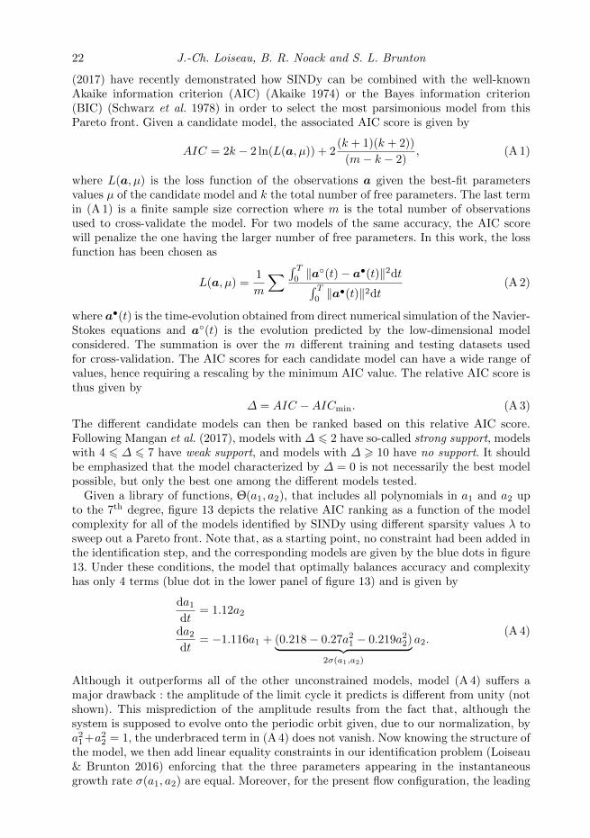
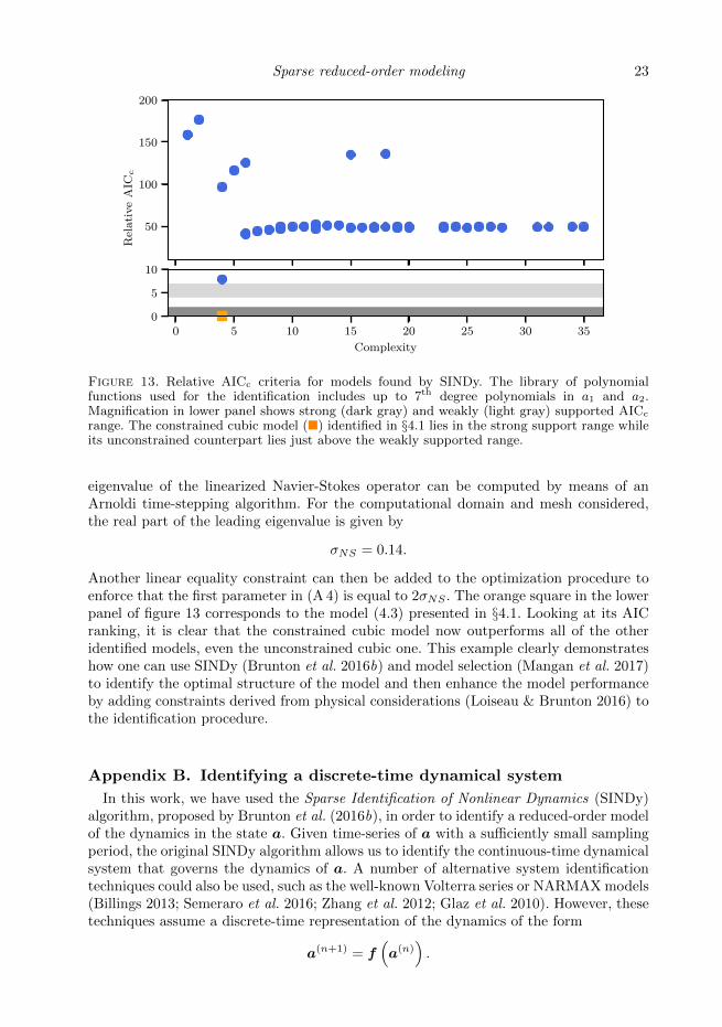
Given a library of functions, Θ(a1, a2), that includes all polynomials in a1 and a2 upto the 7th degree, figure 13 depicts the relative AIC ranking as a function of the modelcomplexity for all of the models identified by SINDy using different sparsity values λ tosweep out a Pareto front. Note that, as a starting point, no constraint had been added inthe identification step, and the corresponding models are given by the blue dots in figure13. Under these conditions, the model that optimally balances accuracy and complexityhas only 4 terms (blue dot in the lower panel of figure 13) and is given by
da1dt
= 1.12a2
da2dt
= −1.116a1 + (0.218− 0.27a21 − 0.219a22)︸ ︷︷ ︸2σ(a1,a2)
a2.(A 4)
Although it outperforms all of the other unconstrained models, model (A 4) suffers amajor drawback : the amplitude of the limit cycle it predicts is different from unity (notshown). This misprediction of the amplitude results from the fact that, although thesystem is supposed to evolve onto the periodic orbit given, due to our normalization, bya21+a22 = 1, the underbraced term in (A 4) does not vanish. Now knowing the structure ofthe model, we then add linear equality constraints in our identification problem (Loiseau& Brunton 2016) enforcing that the three parameters appearing in the instantaneousgrowth rate σ(a1, a2) are equal. Moreover, for the present flow configuration, the leading
Sparse reduced-order modeling 23
0.0 0.2 0.4 0.6 0.8 1.00.0
0.2
0.4
0.6
0.8
1.0
Rel
ativ
eA
ICc
0 5 10 15 20 25 30 35
50
100
150
200
0 5 10 15 20 25 30 35Complexity
0
5
10
Figure 13. Relative AICc criteria for models found by SINDy. The library of polynomialfunctions used for the identification includes up to 7th degree polynomials in a1 and a2.Magnification in lower panel shows strong (dark gray) and weakly (light gray) supported AICc
range. The constrained cubic model (�) identified in §4.1 lies in the strong support range whileits unconstrained counterpart lies just above the weakly supported range.
eigenvalue of the linearized Navier-Stokes operator can be computed by means of anArnoldi time-stepping algorithm. For the computational domain and mesh considered,the real part of the leading eigenvalue is given by
σNS = 0.14.
Another linear equality constraint can then be added to the optimization procedure toenforce that the first parameter in (A 4) is equal to 2σNS . The orange square in the lowerpanel of figure 13 corresponds to the model (4.3) presented in §4.1. Looking at its AICranking, it is clear that the constrained cubic model now outperforms all of the otheridentified models, even the unconstrained cubic one. This example clearly demonstrateshow one can use SINDy (Brunton et al. 2016b) and model selection (Mangan et al. 2017)to identify the optimal structure of the model and then enhance the model performanceby adding constraints derived from physical considerations (Loiseau & Brunton 2016) tothe identification procedure.
Appendix B. Identifying a discrete-time dynamical system
In this work, we have used the Sparse Identification of Nonlinear Dynamics (SINDy)algorithm, proposed by Brunton et al. (2016b), in order to identify a reduced-order modelof the dynamics in the state a. Given time-series of a with a sufficiently small samplingperiod, the original SINDy algorithm allows us to identify the continuous-time dynamicalsystem that governs the dynamics of a. A number of alternative system identificationtechniques could also be used, such as the well-known Volterra series or NARMAX models(Billings 2013; Semeraro et al. 2016; Zhang et al. 2012; Glaz et al. 2010). However, thesetechniques assume a discrete-time representation of the dynamics of the form
a(n+1) = f(a(n)
).
24 J.-Ch. Loiseau, B. R. Noack and S. L. Brunton
Interestingly, the SINDy algorithm described in §3.2 only requires minor modifications inorder to identify such systems. For that purpose, one simply needs to replace the matrixA in the optimization problem by a time-shifted copy of A. Applying this strategy forthe two-dimensional cylinder flow at Re = 100 with a time-lag τ = 0.125 leads to theidentification of the following discrete-time nonlinear dynamical system
[a(n+1)1
a(n+1)2
]=
[0.994 0.139−0.122 1.026
][a(n)1
a(n)2
]
+
[0
−(
0.019a(n)1 + 0.04a
(n)2
)(a(n)1
)2−(
0.017a(n)1 + 0.036a
(n)2
)(a(n)2
)2]. (B 1)
The resulting model can be interpreted as a sparse nonlinear vector autoregressive model(VAR) of the first order. As shown in figure 14, the time evolution of a◦1(t) predictedby this low-dimensional discrete-time system is in good agreement with a•1(t) based ona direct numerical simulation, whose initial condition has been chosen in the vicinity ofthe linearly unstable baseflow.
Based on the continuous-time system (4.3), it thus appears that SINDy can identifyhighly accurate low-order models of the two-dimensional cylinder flow. However, onemay argue that direct numerical simulations only provide ideal noise-free and non-corrupted training data, hence questioning the ability of SINDy to identify similar low-dimensional systems from real-world experimental data. This issue can be addressed bypre-processing the training dataset, such as using a low-pass filter. Alternatively, Bruntonet al. (2016b) used the Total Variation Regularized Numerical Differentiation proposedby Chartrand (2011) in order to evaluate the time-derivative of their noisy data priorto the identification step. Moreover, the SINDy implementation used by Brunton et al.(2016b), Loiseau & Brunton (2016) and herein relies on an iteratively hard-thresholdedleast-square algorithm. As such, one can easily estimate the variance-covariance matrixof the identified model’s parameters in order to estimate its robustness even if noisy dataare used. Finally, it has been shown by Tran & Ward (2016) that SINDy can exactlyrecover the governing equations even if the training data are highly corrupted, providedthe system is sufficiently ergodic or if a sufficient number of different transient trajectorieshave been included in the training dataset.
REFERENCES
Akaike, H. 1974 A new look at the statistical model identification. Automatic Control, IEEETransactions on 19 (6), 716–723.
Arbabi, H. & Mezic, I. 2016 Ergodic theory, Dynamic Mode Decomposition and Computationof Spectral Properties of the Koopman operator. arXiv preprint arXiv:1611.06664 .
Aubry, N., Holmes, P., Lumley, J. L. & Stone, E. 1988 The dynamics of coherent structuresin the wall region of a turbulent boundary layer. J. Fluid Mech. 192, 115–173.
Babaee, H. & Sapsis, T. P. 2016 A variational principle for the description of time-dependentmodes associated with transient instabilities. Phil. Trans. Roy. S. Lond. accepted.
Bagheri, S. 2013 Koopman-mode decomposition of the cylinder wake. J. Fluid Mech 726,596–623.
Balajewicz, M., Dowell, E. H. & Noack, B. R. 2013 Low-dimensional modelling of high-Reynolds-number shear flows incorporating constraints from the Navier-Stokes equation.J. Fluid Mech. 729, 285–308.
Barkley, D. & Henderson, R. D. 1996 Three-dimensional Floquet stability analysis of thewake of a circular cylinder. J. Fluid Mech. 322, 215–241.

Sparse reduced-order modeling 25
0 50 100 150t
−1
0
1
a1
(a)
Raw data a•(t) Discrete-time Model a◦(t)
−1 0 1a2
(b)
Figure 14. (a) Comparison of the evolution as a function of time of the sensor measurement a1obtained from direct numerical simulation (—– a•1) and predicted by the discrete-time sparsemodel (– – a◦1). (b) Trajectory of the true and identified systems in the phase plane (a1, a2). Inboth cases, the initial condition is close to the linearly unstable fixed point.
Barnett, T. P. & Hasselmann, K. 1979 Techniques of linear prediction, with application tooceanic and atmospheric fields in the tropical Pacific. Rev. Geophys. 17, 949–968.
Berkooz, G., Holmes, P. J. & Lumley, J. L. 1993 The proper orthogonal decomposition inthe analysis of turbulent flows. Annual review of fluid mechanics 25 (1), 539–575.
Billings, S. A. 2013 Nonlinear system identification: NARMAX methods in the time, frequency,and spatio-temporal domains. John Wiley & Sons.
Bongard, J. & Lipson, H. 2007 Automated reverse engineering of nonlinear dynamicalsystems. Proceedings of the National Academy of Sciences 104 (24), 9943–9948.
Bourguet, R., Braza, M. & Dervieux, A. 2011 Reduced-order modeling of transonic flowsaround an airfoil submitted to small deformations. J. Comp. Phys. 230, 159–184.
Brunton, S. L., Brunton, B. W., Proctor, J. L., Kaiser, E. & Kutz, J. N. 2017 Chaosas an intermittently forced linear system. Nature Communications 8 (19), 1–9.
Brunton, S. L., Brunton, B. W., Proctor, J. L. & Kutz, J. N 2016a Koopman invariantsubspaces and finite linear representations of nonlinear dynamical systems for control.PLoS ONE 11 (2), e0150171.
Brunton, S. L., Dawson, S. TM & Rowley, C. W. 2014 State-space model identificationand feedback control of unsteady aerodynamic forces. Journal of Fluids and Structures50, 253–270.
Brunton, S. L. & Noack, B. R. 2015 Closed-loop turbulence control: Progress and challenges.Applied Mechanics Reviews 67 (5), 050801.
Brunton, S. L., Proctor, J. L. & Kutz, J. N. 2016b Discovering governing equations fromdata by sparse identification of nonlinear dynamical systems. Proceedings of the NationalAcademy of Sciences 113 (15), 3932–3937.
Brunton, S. L., Proctor, J. L. & Kutz, J. N. 2016c Sparse Identification of NonlinearDynamics with Control (SINDYc). IFAC NOLCOS 49 (18), 710–715.
Brunton, S. L., Rowley, C. W. & Williams, D. R. 2013 Reduced-order unsteadyaerodynamic models at low Reynolds numbers. Journal of Fluid Mechanics 724, 203–233.
Candes, E. J. 2006 Compressive sensing. Proceedings of the International Congress ofMathematics .
Carlberg, K., Barone, M. & Antil, H. 2017 Galerkin v. least-squares Petrov–Galerkinprojection in nonlinear model reduction. Journal of Computational Physics 330, 693–734.
Carlberg, K., Tuminaro, R. & Boggs, P. 2015 Preserving Lagrangian structure in nonlinearmodel reduction with application to structural dynamics. SIAM Journal on ScientificComputing 37 (2), B153–B184.

26 J.-Ch. Loiseau, B. R. Noack and S. L. Brunton
Chartrand, R. 2011 Numerical differentiation of noisy, nonsmooth data. ISRN AppliedMathematics 2011.
Colebrook, J. M. 1978 Continuous plankton records: Zooplankton and environment, NortheastAtlantic and North Sea. Oceanol. Acta 1, 9–23.
Cordier, L., Noack, B. R., Daviller, G., Delvile, J., Lehnasch, G., Tissot, G.,Balajewicz, M. & Niven, R.K. 2013 Control-oriented model identification strategy.Exp. Fluids 54, Article 1580.
Deane, A. E., Kevrekidis, I. G., Karniadakis, G. E. & Orszag, S. A. 1991 Low-dimensional models for complex geometry flows: Application to grooved channels andcircular cylinders. Phys. Fluids A 3, 2337–2354.
Donoho, D. L. 2006 Compressed sensing. IEEE Transactions on Information Theory 52 (4),1289–1306.
Dullerud, Geir. E. & Paganini, F. 2000 A course in robust control theory: A convex approach.Berlin, Heidelberg: Springer.
Duriez, T., Brunton, S. L. & Noack, B. R. 2016 Machine Learning Control–TamingNonlinear Dynamics and Turbulence. Fluid mechanics and its applications (ISSN 0926-5112 116.
Fabbiane, N., Semeraro, O., Bagheri, S. & Henningson, D. S. 2014 Adaptive and model-based control theory applied to convectively unstable flows. Applied Mechanics Reviews66 (6), 060801.
Feynman, R. P., Leighton, R. B. & Sands, M. 2013 The Feynman Lectures on Physics, ,vol. 2. Basic Books.
Fischer, P.F., Lottes, J.W. & Kerkemeir, S.G. 2008 Nek5000 Web pages.Http://nek5000.mcs.anl.gov.
Galletti, G., Bruneau, C. H., Zannetti, L. & Iollo, A. 2004 Low-order modelling oflaminar flow regimes past a confined square cylinder. J. Fluid Mech. 503, 161–170.
Ghil, M., Allen, R. M., Dettinger, M. D., Ide, K., Kondrashov, D. & others 2002Advanced spectral methods for climatic time series. Rev. Geophys. 40, 3.1–3.41.
Glaz, B., Liu, L. & Friedmann, P. P. 2010 Reduced-order nonlinear unsteady aerodynamicmodeling using a surrogate-based recurrence framework. AIAA journal 48 (10), 2418–2429.
Graham, W. R., Peraire, J. & Tang, K. Y. 1999 Optimal control of vortex shedding usindlow-order models. Part I — Open-loop model development. Int. J. Numer. Meth. Engrng.44, 945–972.
Hemati, M. S., Dawson, S. TM & Rowley, C. W. 2016 Parameter-Varying AerodynamicsModels for Aggressive Pitching-Response Prediction. AIAA Journal pp. 1–9.
Holmes, P. J. & Guckenheimer, J. 1983 Nonlinear oscillations, dynamical systems, andbifurcations of vector fields, Applied Mathematical Sciences, vol. 42. Berlin, Heidelberg:Springer-Verlag.
Holmes, P. J., Lumley, J. L., Berkooz, G. & Rowley, C. W. 2012 Turbulence, coherentstructures, dynamical systems and symmetry , 2nd edn. Cambridge, England: CambridgeUniversity Press.
Hosseini, Z., Noack, B. R. & Martinuzzi, R. J. 2016 Modal energy flow analysis of a highlymodulated wake behind a wall-mounted pyramid. J. Fluid Mech. 798, 774–786.
Juang, J.-N. & Pappa, R. S. 1985 An eigensystem realization algorithm for modal parameteridentification and model reduction. Journal of guidance, control, and dynamics 8 (5),620–627.
Kaiser, E., Noack, B. R., Cordier, L., Spohn, A., Segond, M., Abel, M., Daviller, G.,Osth, J., Krajnovic, S. & Niven, R. K. 2014 Cluster-based reduced-order modellingof a mixing layer. J. Fluid Mech. 754, 365–414.
Kalman, R. E. 1960 A new approach to linear filtering and prediction problems. Journal ofFluids Engineering 82 (1), 35–45.
Krizhevsky, A., Sutskever, I. & Hinton, G. E. 2012 Imagenet classification with deepconvolutional neural networks. In Advances in neural information processing systems, pp.1097–1105.
Kutz, J. N. 2017 Deep learning in fluid dynamics. Journal of Fluid Mechanics 814, 1–4.
Sparse reduced-order modeling 27
Kutz, J. N., Brunton, S. L., Brunton, B. W. & Proctor, J. L. 2016 Dynamic ModeDecomposition: Data-Driven Modeling of Complex Systems. SIAM.
Lee, C., Kim, J., Babcock, D. & Goodman, R. 1997 Application of neural networks toturbulence control for drag reduction. Physics of Fluids 9 (6), 1740–1747.
Ling, J., Kurzawski, A. & Templeton, J. 2016 Reynolds averaged turbulence modellingusing deep neural networks with embedded invariance. Journal of Fluid Mechanics 807,155–166.
Loiseau, J.-Ch. & Brunton, S. L. 2016 Constrained sparse Galerkin regression. arXiv preprintarXiv:1611.03271 .
Mangan, N. M., Brunton, S. L., Proctor, J. L. & Kutz, J. N. 2016 Inferring biologicalnetworks by sparse identification of nonlinear dynamics. IEEE Transactions on Molecular,Biological, and Multi-Scale Communications 2 (1), 52–63.
Mangan, N. M., Kutz, J. N., Brunton, S. L. & Proctor, J. L. 2017 Model selectionfor dynamical systems via sparse regression and information criteria. arXiv preprintarXiv:1701.01773 .
Mantic-Lugo, V., Arratia, C. & Gallaire, F. 2014 Self-consistent mean flow descriptionof the nonlinear saturation of the vortex shedding in the cylinder wake. Physical reviewletters 113 (8), 084501.
McConaghy, T. 2011 Ffx: Fast, scalable, deterministic symbolic regression technology. InGenetic Programming Theory and Practice IX , pp. 235–260. Springer.
Mezic, I. 2005 Spectral properties of dynamical systems, model reduction and decompositions.Nonlinear Dynamics 41 (1-3), 309–325.
Mezic, I. 2013 Analysis of fluid flows via spectral properties of the Koopman operator. AnnualReview of Fluid Mechanics 45, 357–378.
Milano, M. & Koumoutsakos, P. 2002 Neural network modeling for near wall turbulent flow.Journal of Computational Physics 182 (1), 1–26.
Nair, A. G. & Taira, K. 2015 Network-theoretic approach to sparsified discrete vortexdynamics. Journal of Fluid Mechanics 768, 549–571.
Noack, B. R. 2016 From snapshots to modal expansions – bridging low residuals and purefrequencies. J. Fluid Mech. – Focus in Fluids 802, 1–4.
Noack, B. R., Afanasiev, K., Morzynski, M., Tadmor, G. & Thiele, F. 2003 A hierarchyof low-dimensional models for the transient and post-transient cylinder wake. J. FluidMech. 497, 335–363.
Noack, B. R., Morzynski, M. & Tadmor, G. 2011 Reduced-order modelling for flow control.,, vol. 528. Springer Science & Business Media.
Noack, B. R., Stankiewicz, W., Morzynski, M. & Schmid, P. J. 2016 Recursive dynamicmode decomposition of transient and post-transient wake flows. J. Fluid Mech. 809, 843–872.
Osth, J., Krajnovic, S., Noack, B. R., Barros, D. & Boree, J. 2014 On the need fora nonlinear subscale turbulence term in POD models as exemplified for a high Reynoldsnumber flow over an Ahmed body. J. Fluid Mech. 747, 518–544.
Rediniotis, O.K., Ko, J. & Kurdila, A.J. 2002 Reduced order nonlinear Navier-Stokesmodels for synthetic jets. J. Fluids Enrng. 124 (2), 433–443.
Rempfer, D. 2000 On low-dimensional Galerkin models for fluid flow. Theoret. Comput. FluidDynamics 14, 75–88.
Rempfer, D. & Fasel, F. H. 1994 Dynamics of three-dimensional coherent structures in aflat-plate boundary-layer. J. Fluid Mech. 275, 257–283.
Rowley, C. W. & Dawson, S. 2016 Model reduction for flow analysis and control. AnnualReview of Fluid Mechanics 49 (1).
Rowley, C. W., Mezic, I., Bagheri, S., Schlatter, P. & Henningson, D.S. 2009 Spectralanalysis of nonlinear flows. J. Fluid Mech. 645, 115–127.
Rudy, S. H., Brunton, S. L., Proctor, J. L. & Kutz, J. N. 2017 Data-driven discovery ofpartial differential equations. Science Advances 3 (e1602614).
Schaeffer, H. 2017 Learning partial differential equations via data discovery and sparseoptimization. In Proc. R. Soc. A, , vol. 473, p. 20160446.
Schlegel, M. & Noack, B. R. 2015 On long-term boundedness of galerkin models. Journalof Fluid Mechanics 765, 325–352.
28 J.-Ch. Loiseau, B. R. Noack and S. L. Brunton
Schmid, P. J. 2010 Dynamic mode decomposition of numerical and experimental data. Journalof Fluid Mechanics 656, 5–28.
Schmidt, M. & Lipson, H. 2009 Distilling free-form natural laws from experimental data.science 324 (5923), 81–85.
Scholkopf, B., Smola, A. & M uller, K.-R. 1998 Nonlinear component analysis as a kerneleigenvalue problem. Nerual Computation 10, 1299–1319.
Schumm, M., Eberhard, B. & Monkewitz, P. A. 1994 Self-excited oscillations in the wakeof two-dimensional bluff bodies and their control. J. Fluid Mech. 271, 17–53.
Schwarz, G. & others 1978 Estimating the dimension of a model. The annals of statistics6 (2), 461–464.
Semeraro, O., Lusseyran, F., Pastur, L. & Jordan, P. 2016 Qualitative dynamics ofwavepackets in turbulent jets. arXiv preprint arXiv:1608.06750 .
Sengupta, T. K., Haider, S. I., Parvathi, M. K. & Pallavi, G. 2015 Enstrophy-basedproper orthogonal decomposition for reduced-order modeling of flow past a cylinder.Physical Review E 91 (4), 043303.
Sipp, D. & Schmid, P. J. 2016 Linear closed-loop control of fluid instabilities and noise-induced perturbations: A review of approaches and tools. Applied Mechanics Reviews68 (2), 020801.
Sirovich, L. 1987 Turbulence and the dynamics of coherent structures. Part I: Coherentstructures. Quarterly of Applied Mathematics 45 (3), 561–571.
Skogestad, S. & Postlethwaite, I. 2005 Multivariable feedback control: analysis and design,2nd edn. Hoboken, New Jersey: John Wiley & Sons, Inc.
Tadmor, G., Lehmann, O., Noack, B. R., Cordier, L., Delville, J., Bonnet, J.-P. &Morzynski, M. 2011 Reduced order models for closed-loop wake control. PhilosophicalTransactions of the Royal Society A 369 (1940), 1513–1524.
Tadmor, G., Lehmann, O., Noack, B. R. & Morzynski, M. 2010 Mean field representationof the natural and actuated cylinder wake. Physics of Fluids (1994-present) 22 (3), 034102.
Takens, F. 1981 Detecting strange attractors in turbulence. In Dynamical systems andturbulence, Warwick 1980 , pp. 366–381. Springer.
Tibshirani, R. 1996 Regression shrinkage and selection via the lasso. Journal of the RoyalStatistical Society. Series B (Methodological) pp. 267–288.
Tran, G. & Ward, R. 2016 Exact Recovery of Chaotic Systems from Highly Corrupted Data.ArXiv e-prints , arXiv: 1607.01067.
Tu, J. H., Rowley, C. W., Luchtenburg, D. M., Brunton, S. L. & Kutz, J. N. 2014On dynamic mode decomposition: theory and applications. Journal of ComputationalDynamics 1 (2), 391–421.
Ukeiley, L., Cordier, L., Manceau, R., Delville, J., Bonnet, J. P. & Glauser, M. 2001Examination of large-scale structures in a turbulent plane mixing layer. Part 2. Dynamicalsystems model. J. Fluid Mech. 441, 61–108.
Wang, W. X., Yang, R., Lai, Y. C., Kovanis, V. & Grebogi, C. 2011 Predictingcatastrophes in nonlinear dynamical systems by compressive sensing. Physical ReviewLetters 106, 154101–1–154101–4.
Weare, B. C. & Nasstrom, J. N. 1982 Examples of extended empirical orthogonal functionanalyses. Mon. Weather Rev. 110, 784–812.
Wei, M. & Rowley, C. W. 2009 Low-dimensional models of a temporally evolving free shearlayer. J. Fluid Mech 618, 113–134.
Welch, G. & Bishop, G. 1995 An introduction to the Kalman filter.
Wiener, N. 1948 Cybernetics or Control and Communication in the Animal and the Machine,1st edn. Boston: MIT Press.
Williams, M. O., Kevrekidis, I. G. & Rowley, C. W. 2015 A data-driven approximationof the Koopman operator: extending dynamic mode decomposition. Journal of NonlinearScience .
Zebib, A. 1987 Stability of viscous flow past a circular cylinder. Journal of EngineeringMathematics 21 (2), 155–165.
Zhang, H.-Q., Fey, U., Noack, B. R., Konig, M. & Eckelmann, H. 1995 On the transitionof the cylinder wake. Physics of Fluids (1994-present) 7 (4), 779–794.

Sparse reduced-order modeling 29
Zhang, W., Wang, B., Ye, Z. & Quan, J. 2012 Efficient method for limit cycle flutter analysisbased on nonlinear aerodynamic reduced-order models. AIAA journal 50 (5), 1019–1028.
Zhang, Z. J. & Duraisamy, K. 2015 Machine learning methods for data-driven turbulencemodeling. In 22nd AIAA Computational Fluid Dynamics Conference, p. 2460.