Reduced order borehole induction modellingN. Ardjmandpour1, C. Pain2, F. Fang2, J. Singer1, M. A. Player1, Xu Xu1, I. M. Navon3, J.

Carter2

1 GE Energy Oilfield Technology, Building X 107, Range Road, Cody Technology Park, Farnborough, Hampshire,

GU14 0FG, UK

2 Department of Earth Science and Engineering, Imperial College London, South Kensington Campus, ExhibitionRoad, London SW7 2AZ, UK

3 Department of Scientific Computing, Florida State University, Tallahassee, FL 32306-4120, U.S.A.

SUMMARY

The development of the reduced order model, Proper Orthogonal Decomposition (POD) method,for array induction tool has been demonstrated in this paper for the first time. The motivationbehind the reduced order modelling is that numerical simulation of Maxwell equations is tooexpensive in terms of computational time for the purpose of inversion, where the forward modelneeds to be run many times. In this study, we demonstrate that the POD model is fast and accu-rate for an iterative inversion to estimate the formation conductivity. The POD method optimallyextracts a few fundamental modes or basis functions from the numerical/experimental solutions,that can accurately represent the most energy in the original dynamic system. The solutions canbe reconstructed as a linear combination of the POD basis functions through Galerkin projec-tion. POD provides a low-dimensional description of the system’s dynamics, which is an orderof magnitude smaller than the dimension of the full forward model. The POD model is appliedto the numerical solutions obtained from a finite element forward model. The results show thatthe POD solutions agree well with the ones obtained from the forward model.

Key words: POD, reduced order model, array induction tool, Maxwell equations.

1 Introduction

The goal of processing induction log signals is to invert measured responses and obtain theestimates of the true formation conductivity profiles. The conductivity can be used to infer thefluid content of geological formations, where lower conductivity (higher resistivity) is typicallyassociated with those formations that bear hydrocarbons.

When inverting the measured induction log signal to estimate the formation conductivity, oneuses an iterative optimization technique based on a forward model. However, the use of a

1

forward model based on the solution of the partial differential equation (PDE) using an approachsuch as Finite Element (FE) is very expensive in terms of the computer time (Lin et al., 1984).Anderson and Gianzero (1983) developed a 1D spectral integral code which computes inductionresponse in an arbitrary number of planar layered media. Although their fast forward model cansignificantly improve the speed compared to the forward model with FE method (Lin et al.,1984; Dyos, 1987; Freedman and Minerbo, 1991), these models are still not fast enough fordetermination of inversions that could lead to well-site identification. The approximation to theforward model such as Born approximation (Thadani et al., 1983) based on geometrical factortheory (Doll, 1949; Moran, 1982), could considerably speed up the inversion process (Dyos,1987; Freedman and Minerbo, 1991). The drawback of this approximation is that it breaks downfor high conductivity beds or where there are large contrasts in the formation conductivity.

To speed up the inversion process, one can replace the forward model by a fast forward modelsuch as a neural network, where the layer conductivities are inputs and the array responsesare the output. In this case, a large quantity of training data is required in order to cover thecombinations and ranges of conductivities on the layer media. However, even if we use thetechnique developed for the efficient collection of training data (Ardjmandpour, 2010), it maynot be practical to obtain sufficient data. To tackle this problem, one can use model reductiontechniques to lessen memory and computational costs as demonstrated in this paper using theproper orthogonal decomposition (POD) method.

The POD method optimally extracts the fewest most energetic modes or basis functions fromthe numerical/experimental solutions that can accurately represent the system dynamic. PODwas invented by Pearson (1901). Proper orthogonal decomposition is also known as principlecomponent analysis (Kosambi, 1943; Fukunaga, 1990) in statistics, or Karhunen-Loeve decom-position (Loeve, 1945; Karhunen, 1946), and empirical orthogonal functions (EOF) in oceanog-raphy (Jolliffe, 2002; Crommelin and Majda, 2004) and meteorology (Majda et al., 2003).

The POD methodologies, in combination with the Galerkin projection procedure, have addi-tionally provided an efficient means of generating reduced-order models (Holmes et al., 1998;Kunisch and Volkwein, 2003; Luo et al., 2007). This technique can provide a low dimensionalordinary differential equation (ODE) as an approximation to the PDE models. Basically thePDE’s are solved for different parameter values to extract an ensemble of forward solutions,referred to as snapshots. The POD basis functions are obtained by applying a singular valuedecomposition (SVD) analysis to the snapshots. The Galerkin method is then used to projectthe PDE onto the reduced POD basis functions. To improve the accuracy of reduced models,a goal-oriented approach has been used to optimize the POD basis functions (Willcox et al.,2005; Bui-Thanh et al., 2007).

POD has been used successfully in several fields, such as fluid dynamics and coherent structures(Lumley, 1967; Aubry et al., 1988; Holmes et al., 1998; Willcox and Peraire, 2002), signal pro-cessing and pattern recognition (Fukunaga, 1990), image reconstruction (Kirby and Sirovich,

2

1990), inverse problems (Vauhkonen et al., 1997; Banks et al., 2000; Hopcroftand et al., 2009)and ocean modelling with the four-dimentional variational (4D-Var) data assimilation technique(Robert et al., 2005; Hoteit and Khl, 2006; Luo et al., 2007; Fang et al., 2009). In this paper, wepropose to use the POD method for downhole measurements for the first time.

The COMSOL forward model 1 is used to generate snapshots, which are sampled at differentconductivities. The solutions/snapshots, which are the azimuthal magnetic vector potentials,are stored in a data matrix, where each column represents the solution at each conductivity. ThePOD procedure is then used to extract the few most energetic modes/basis functions from thedata matrix. The POD reduced model is then derived using Galerkin projection of the PODbasis functions onto the governing equation used by COMSOL, which leads to the POD coef-ficients. Finally, the data matrix can be reconstructed with the use of the POD basis functionsand coefficients. In order to construct the POD model, the numerical technique introduced byFang et al. (2009, 2010) is used, whereby the POD forward model can be constructed by us-ing the system matrices derived from the full model. The main advantages of POD are; i) itrequires standard matrix computations and ii) it can applied to nonlinear problems (Schilderset al., 2008).

The POD basis functions are derived from snapshots using SVD. The POD basis functionsare only able to give an optimal representation of the energy included in the snapshot sets.Therefore, the effectiveness of the POD basis rely on the generation of good snapshot sets(Gunzburger, 2003). Although, there are some methods such as the dual-weighed approach(Daescu and Navon, 2008; Chen et al., 2009) which can be used to select the snapshots, thechoice and number of the snapshots are problem dependent and mostly rely on knowledgeof the solution of the original physical system. In this study, snapshots are generated usinga layered model in which the conductivity varies only with depth. The number of snapshotschosen is based on the fractional factorial design (Xu, 2005).

The reminder of this paper is structured as follows: In section 2, a brief introduction to thetheory of array induction tools is given, followed by a brief description of the governing equa-tions used in simulating the array induction tool responses. A brief review of POD is givenin section 3. The reduced forward model is then derived, followed by a detailed descriptionof mathematical procedure used to solve the POD model. Finally, the results are presented insection 4.

1http://www.comsol.com

3

2 Induction Tools

Fundamental aspects

Commercial induction tools are normally composed of several transmitter and receiver coilswhich are designed to optimize vertical resolution and depth of investigation. The basic elementin an induction tool is the two-coil sonde, which consists of a transmitter and receiver mountedcoaxially on a mandrel (Figure 1). The constant-amplitude alternating current in the transmittercoil sets up a primary electromagnetic field around the tool. The primary electromagnetic fieldinduces eddy currents (often called “ground loops”) in the formation. The eddy currents, whichflow coaxially to the borehole and the intensity of which are proportional to conductivity of theformation, in turn induce a secondary voltage in a receiver coil. The voltage induced in thereceiver directly from the transmitter coil is bucked-out using bucking coils, so that only thesecondary voltages can be investigated.

The induced secondary voltage is due to the sum of all the eddy current loops with radius r, atdepth z, weighted by geometrical factors to allow for their radial distance r from the borehole,and the vertical distance z above or below the transmitter. The induced secondary voltage is out-of-phase with the transmitter current, and therefore has both a real and an imaginary component.A complex conductivity for the formation can be obtained by dividing measured voltage by theK factor, which is a tool constant containing information about dimensions of transmitter andreceiver (Moran and Kunz, 1962).

However, the measured signal is effected by the logging environment (Figure 2) such as

• Borehole effects: the conductivity of the mud and borehole size can affect the accuracyof the measurements; i.e. the influence of the borehole increases with mud conductivityand borehole diameter.

• Mud filtrate invasion: in permeable formations, responses are influenced by the spatialdistribution of fluids/hydrocarbons in the vicinity of the borehole resulting from the inva-sion of mud filtrate.

• Shoulder effects: the conductivity/resistivity of the formation layers above and below abed/layer of interest, referred as shoulder beds, can also effect the measurement.

• Dipping beds: the relative dip between the tool and formation can affect the tool re-sponses, e.g. the effect of high relative dip angle is to blur the response and to introducehorns at the bed boundaries (Barber et al., 1999).

To accurately estimate the formation conductivity, one needs to correct the measurements forthese effects. Traditional method for correction involved applying a series of corrections chart (Rust

4

and Anderson, 1975; Anderson, 2001; Hardman and Shen, 1987). However, the accuracy of theresults largely relied on the experience of the log analyst. On the other hand, the manual cor-rections for the induction tools such as array tools (Hunka et al., 1990; Barber et al., 1995)with more measurements are time consuming. In the mid 1980’s, the development of computermodelling made it possible for the log analyst to use correction algorithms based on forwardmodelling (Anderson, 2001).

Grove and Minerbo, in 1991, designed a correction algorithm to solve for borehole parametersby minimizing the difference between the model and measured signals from array inductiontool. The borehole corrected signals are then combined to form the log responses which havethe desired vertical response, radial response and a smooth near-borehole 2D response (Bar-ber and Rosthal, 1991; Ellis and Singer, 2007). Then a 2D inversion can be used to estimatethe formation conductivity and invasion parameters; i.e. invasion conductivity and invasion ra-dius (Howard, 1992). In horizontal and deviated wells, the dip correction algorithms, based onfiltering (Xiao et al., 2000) or iterative inversion (Barber et al., 1999) can be used to remove thedip effects.

However, the 2D inversion is slow because the nonlinearity of the problem leads to severaliterations through the model for each interval. The process can be speeded up by dividing theproblem into a sequence of 1D inverse problems, such as first determining vertical layers andthen invasion depth (Lin et al., 1984; Dyos, 1987; Freedman and Minerbo, 1991; Anderson,2001; Ellis and Singer, 2007). This can significantly reduce the computation time.

Assuming we can neglect invasion and dip effects, a 1D inversion can be used to estimate theconductivity in a layered medium. In this study, we introduce a fast surrogate model POD topredict the array response for a layered media. We demonstrate that the POD model is fastand accurate for an iterative inversion to estimate the formation conductivity. In this study themethod is applied to the two-coil sonde. The method has been expanded for the multi arrayinduction tool (Ardjmandpour, 2010).

Governing equation

COMSOL Multiphysics is a simulator software that uses Finite-Element models (FEM) to com-pute the array response. COMSOL uses a built-in formulation of the time harmonic Quasi-staticelectromagnetic equation. The partial differential equation, in 2D modelling, solved by COM-SOL can be expressed as:

(iωσ−ω2ε0εr

)Aφ +∇×

(µ−1

0 µ−1r ∇×Aφ

)= Je

φ, (1)

where ω is the frequency of the current, µr is the relative magnetic permeability of the formation,σ is the formation conductivity, ε0 is the dielectric permittivity of free space, εr is relative

5

dielectric permittivity, µ0 is magnetic permeability of free space, Aφ is the azimuthal vectorpotential and Je

φ is the azimuthal component of external current density.

The voltage induced in the receiver coils is computed using the relation, E = iωAφ. For areceiver coil of radius ρ with NR turns, the induced voltage is calculated as follows:

V = 2πρNRE = 2πρNRiωAφ. (2)

The discrete model of equation 1 can be written in a general form as follows:

E(σ)Aφ = b, (3)

where E(σ) is the matrix including all the discretisation of equation 1 and b includes a discre-tised source term. The dimension of equation 3 is N×N where N is the number of grid pointsin the numerical model, e.g. for the data studied N = 111081. In the following subsections, weexplain the mathematical procedure used to derive a low dimensional model of equation 3 usingthe POD approach.

3 POD reduced model

The solutions/snapshots obtained from the original full model are stored in the data matrix Awith dimension N×K, where K is the number of snapshots (typically K ¿ N). The average ofthe ensemble of snapshots is defined as:

Ai =1K

K

∑k=1

Ai,k, 1≤ i≤ N. (4)

Then, a new data matrix is formed by subtracting the mean Ai from each snapshot (Mirandaet al., 2008):

Ci,k = Ai,k− Ai. (5)

The goal of POD is to find a set of orthogonal basis functions Φ = Φ1,Φ2, · · · ,ΦK , such that itmaximises:

6

1K

K

∑k=1

N

∑i=1

(CikΦk)2, (6)

subject to:

K

∑k=1

Φ2k = 1. (7)

The optimal POD basis functions Φk are computed by forming the singular value decomposi-tion (SVD) of the matrix C ∈ RN×K:

C = X ∆ UT , (8)

where diagonal entries of ∆ = diag(σ1, σ2, · · · , σk) are the singular values, X =(Φ1,Φ2, · · · ,ΦN)and, U = (u1,u2, · · · ,uK) are the matrices which consist of orthogonal vectors for CCT and CTCrespectively. In order to obtain the POD basis, we need to solve CCT . This matrix has a dimen-sion of N×N, therefore an eigen decomposition of this matrix will be very computationallyexpensive. Therefore the K×K eigenvalue problem is solved as:

CTCuk = λkuk; 1≤ k ≤ K, (9)

where λk = σ2k are real and positive and should be sorted in a descending order. In this case,

the singular value decomposition is equivalent to the eigenvalue decomposition. The POD basisfunctions Φ are then calculated as follows:

Φk = Cik uk/√

λk. (10)

The kth eigenvalue is a measure of the kinetic energy transferred within the kth basis mode(Fang et al., 2009). Since eigenvalues are arranged in descending order, we can choose thefirst M POD basis functions corresponding to the largest eigenvalues and neglect eigenvaluespossessing small amounts of energy. The energy associated with the M basis functions can bequantified as EM = ∑M

m=1 λm. The total energy of the system is obtained by Et = ∑Kk=1 λk. The

relative energy captured by the Mth basis functions is given by:

7

I(M) =EM

Et, (11)

M can be chosen to capture the desired level of energy. There are other criteria which can beused to select M; e.g. the rate of decay of λk with increasing k, or through an iterative processby minimizing the error between the reduced order model and the full model (Cardoso andDurlofsky, 2010).

The POD basis functions are then used to reconstruct the data matrix as follows:

APODi,k = Ai +

M

∑m=1

Φi,mam,k, (12)

where a are POD coefficients and are determined by solving the forward model in the reducedspace. To calculate POD coefficients, we use the Galerkin projection, in which the POD basisfunctions are used as a basis to solve the full model. The procedure involves substituting thePOD solution (equation 12) into the full forward model and taking the POD basis function asthe test function, then integrating over the computational domain. The result of this procedureis a conductivity-dependent ordinary differential equation of an order equal to the number ofthe POD basis functions M. In this study, we solve the discrete representation of the ODE inwhich the system matrices are obtained by projecting the system matrices of the full forwardmodel (E and b in equation 3) onto the POD basis. In the following subsections, each step ofthe approach will be explained in detail.

3.1 Discrete POD model for array induction measurement

The POD model is derived by substituting equation 12 into equation 1 and taking the POD basisfunction as the test function, then integrating over the computational domain, yielding:

∫

ΩΦ j((iωσ−ω2ε0εr)(A+

M

∑m=1

am Φm(x)) +

∇× (µ−10 µ−1

r ∇× (A+M

∑m=1

am Φm(x)))− Jeφ)dΩ = 0, (13)

where A is the mean value of the ensemble of snapshots, and in the finite element method, thePOD basis Φm(x) = ∑N

i=1 NiΦmi. The discrete model of equation 13 can be written in a generalform as:

8

E(σ)a = b, (14)

where E(σ) is the matrix including all the discretisation of equation 13 and b is including adiscretised source term and the terms corresponding to the mean values (detailed explanationin section 3.2). E(σ) and b can be calculated by projecting E and b onto the basis functions asfollows:

E(σ) = ΦT E(σ)Φ,

b = ΦT b. (15)

Therefore, the entry of the matrix E(σ) can be constructed by the entries of the matrix E (Fanget al., 2010) as:

Eml(σ) =N

∑p=1

N

∑q=1

Epq(σ)Φm pΦl q, (16)

bm =N

∑p=1

bpΦm p, (17)

where Epq(σ) is the (p,q)th entry of the matric E (equation 3) and bp is the pth entry of b (equa-tion 3).

In order to solve equation 14, one needs to derive the vector b and the system matrix E(σ)for each value of conductivity. However, calculating E(σ) for each value of conductivity, ateach finite element and node over the computational domain is a time consuming process. Toovercome this problem, we construct the matrix E(σ) by a set of sub-matrices independent ofconductivity, as follows (Fang et al., 2009, 2010):

E(σ) = E0 +L

∑l=1

σl(E l1−E0), (18)

where E l1 and E0 are derived from equation 1, when σ = 1 and σ = 0 respectively and l is the

number of vertical layers considered in the model. Therefore, instead of calculating matrix Efor each value of the conductivity, one needs to extract the sub-matrices E0 and E1 once prior tothe POD calculations.

9

3.2 Forming the discrete POD model

This section explains how to solve the discrete POD model (equation 14). Since the forwardmodel is complex, the discrete POD model is also complex, and can be written in a complexform as follows:

(P+ i Q)(aR + i aI) = (bR + i bI),

in a matrix form:

(P −QQ P

)(aR

aI

)=

(bR

bI

), (19)

where P and Q are the real and imaginary parts of the matrix E, respectively. The subscript ′R′

refers to the real part and the subscript ′I′ refers to the imaginary part.

To solve equation 19, first the POD basis functions are used to project the system to reducedspace (equation 15). In order to obtain precise estimation of the complex solution, the PODbasis are calculated for the real and imaginary parts separately. Therefore, the POD procedureis applied as follows:

• First, the data matrix C is constructed for the real and imaginary parts

CR = AR− AR; real part,

CI = AI− AI; imaginary part, (20)

where AR and AI are the real and imaginary parts of the snapshots and (AR) and (AI) arethe mean value of real and imaginary parts calculated using equation 4 respectively.

• Then the singular value decomposition is applied to CR and CI separately, leading to thePOD basis for real (ΦR) and imaginary (ΦI) parts.

Once the POD basis functions (ΦR and ΦI) are obtained, the left hand side (E) and the righthand side (b) of equation 19 can be calculated as follows:

Calculating matrix E

Considering equation 15:

10

E(σ) = ΦT E(σ)Φ, (21)

Substituting E =

(P −QQ P

), where P and Q are the real and imaginary parts of the matrix E

and POD basis functions Φ =

(ΦR 00 ΦI

)in equation 21, yields:

(ΦT

RPΦR −ΦTRQΦI

ΦTI QΦR ΦT

I PΦI

). (22)

Taking into account equation 18, matrix E can be constructed as follows:

(ΦT

R P0ΦR +∑Ll=1 σl(ΦT

R Pl1ΦR−ΦT

R P0ΦR) −(ΦTR Q0ΦI +∑L

l=1 σl(ΦTR Ql

1ΦI −ΦTR Q0ΦI))

ΦTI Q0ΦR +∑L

l=1 σl(ΦTI Ql

1ΦR−ΦTI Q0ΦR) ΦT

I P0ΦI +∑Ll=1 σ(ΦT

I Pl1ΦI −ΦT

I P0ΦI)

), (23)

where P0 and Q0 are the real and imaginary parts of E0 and P1 and Q1 are the real and imaginaryparts of E1 respectively.

Calculating b

The vector b includes a discretised source term and terms corresponding to the mean values isexpressed as:

b = ΦT (b−E(σ)A), (24)

The second term can be written in a matrix form as:

(ΦT

RPAR−ΦTRQAI

ΦTI QAR +ΦT

I PAI

)real part

imaginary part(25)

The first term is real, therefore the equation 24 can be expressed as:

ΦT

Rb−ΦTRPAR +ΦT

RQAI

−ΦTI QAR−ΦT

I PAI

. (26)

11

Taking into account equation 18, the vector b can be constructed as follows:

(ΦT

R b− (ΦT

R P0AR +∑Ll=1 σl(ΦT

R Pl1AR−ΦT

R P0AR))+

(ΦT

R Q0AI +∑Ll=1 σl(ΦT

R Ql1AI −ΦT

R Q0AI))

−(ΦT

I P0AI +∑Ll=1 σl(ΦT

I Pl1AI −ΦT

I P0AI))− (

ΦTI Q0AR +∑L

l=1 σl(ΦTI Ql

1AR−ΦTI Q0AR)

).

)

(27)

The coefficients aI and aR are then calculated by substituting equations 23 and 27 into equa-tion 19. The dimension of the POD reduced model (equation 19) is 2M× 2M. Since M ¿ N,the POD model has a much smaller dimension than the full model (equation 3).

To speed up the POD simulation, the sub-matrices; (ΦTRP0ΦR, ΦT

RPl1ΦR, ΦT

RQ0ΦI , ΦTRQl

1ΦI ,ΦT

I Q0ΦR, ΦTI Ql

1ΦR, ΦTI P0ΦI and ΦT

I Pl1ΦI) in equation 23 and (ΦT

RP0A, ΦTRPl

1A, ΦTRQ0AI ,

ΦTRQl

1AI , ΦTI P0AI , ΦT

I Pl1AI and ΦT

I Ql1) in equation 27 are calculated once prior to the POD

calculations; with a dimension of M which is much smaller than dimension N of P0, Q0, P1 andQ1. Therefore a POD simulation can be run in a few seconds. This significantly speeds up thePOD calculation, especially in inverse problems, where the POD forward model needs to be runmany times.

3.3 POD solution

The solution of the reduced order model a can then be converted back to a FE nodal vector byusing the POD basis functions. The POD solution of the azimuthal vector potential for real andimaginary parts can be obtained as follows:

APODR (x,σ) = AR +ΦT

RaR; real part,

APODI (x,σ) = AI +ΦT

I aI; imaginary part. (28)

4 Numerical experiments

In this section, the POD method is applied to the array induction measurements. Snapshotsare generated by running COMSOL for different values of conductivities. The formation ismodelled as a layered medium in which the conductivity varies only with depth. The PODbasis functions are calculated based on singular value decomposition. The POD coefficientsare calculated by solving the POD discrete model using the POD basis functions, leading to thereconstruction of the snapshots.

12

Generation of Snapshots

In order to generate the required snapshots for POD calculation, COMSOL simulation is used.A 5 layered model, as depicted in Figure 3, with the computational domain size 4m×2m, with10929 triangular elements and 111081 nodes in the model, is set up for array 1. We assumethat there is no invasion and data has been corrected for borehole effect, therefore the boreholeis not included in the model. The thickness of each layer is 0.07 m (3 inch). The transmittercoil (Tx) and main receiver (RxM) are located at the same distance from the center; the Txcoil is situated within the layer 2 and Main (RxM) and Bucking (RxB) coils are located 0.15 mand 0.1 m respectively from the source. The upper and lower sections of formation (“layer 0”and “layer 6”) have a fixed background conductivity of 0.016 S/m. The solution is calculatedas the azimuthal component of magnetic vector potential Aφ, the model imposes the Dirichletboundary conditions Aφ = 0 on the symmetry axis.

Snapshots are generated for different values of conductivities for each layer. The layer con-ductivities should be chosen in a way that can represent the values encountered in the actualformation, i.e. values between 0.001 S/m and 1 S/m. To achieve this, low (L), medium (M)and high (H) values of σ, in the range of 0.001-1 S/m, with the contrast 1:10 are chosen, i.e.L=0.001 S/m, M=0.03 S/m and H=1 S/m. The 27 combinations of L, M and H values of σ for5 layers are chosen based on fractional factorial design (Xu, 2005). The design of 27 runs usedto generate the snapshots is summarised in Table 1.

POD basis

The ensemble of snapshots C are constructed for the real and the imaginary parts (equation 20)separately. The ARPACK (Lehoucq et al., 1998), which is a collection of Fortran 77 subroutinesthat is designed to solve large scale eigenvalue problems, is then used to compute the eigenval-ues and eigenvectors. Figure 4 shows the percentage energy (equation 11) captured by differentnumbers of POD basis functions. 5 POD basis functions can capture about 98% of the energyfrom the imaginary part and 86.68% from the real part. As can be seen, the more POD basisfunctions that are chosen, the better the % energy capture. The aim is to choose the minimumnumber of the POD basis which can capture most of the energy. In our case, 20 POD basisfunctions are chosen which can capture 99% of the energy from the real part and 99.99% of theenergy from the imaginary part.

POD solution method

To solve the discrete POD model (section 3.2), the required system matrices (E0 and E l1 where

l = 1,2,3, · · · ,5) are derived from the full forward model as follows:

13

1. E0 is obtained from discretization of equation 1 where the conductivity of all 5 layers isequal to zero.

2. E11 is obtained where the conductivity corresponding to layer l is equal to 1 and other

layers is equal to 0. For example for l=1 the conductivity of layer 1 is equal to 1 andlayers 2 to 5 are equal to 0.

In total, the matrices (E0,E1,E2,E3,E4,E5) and the vector b are extracted from the discretiza-tion of the full model (equation 1). These matrices and the vector b are used to construct E(equation 23) and b (equation 27), leading to solution of the discrete POD model (equation 14).The dimension of the reduced order model is 40, which is several orders of magnitude smallerthan the dimension of the full model of 111081.

4.1 Results

Figures 5 to 8 show the POD solution of the azimuthal vector potential. Figures 5 and 6 illus-trate the results for one of the snapshots which is used to calculate the POD basis functions (seencase) with conductivities of 0.03 S/m, 0.03 S/m, 0.001 S/m, 1 S/m, 0.001 S/m corresponding tolayers 1 to 5 respectively. The results show that the POD solutions for both real and imaginaryparts are in good agreement with those from the COMSOL. Figures 7 and 8 show the results ofreal and imaginary parts for a case, which is not used in determining the POD basis functions(we call it unseen case). The conductivities of each layer are 0.025 S/m, 0.033 S/m, 0.08 S/m,0.09 S/m, and 0.09 S/m, from layers 1 to 5 respectively. The results for both seen and unseencases show that the POD results agree well with those from the COMSOL. The maximum abso-lute difference errors between the COMSOL and POD solution, for both seen and unseen cases,are less than 0.4×10−11 S/m for real part and 0.4×10−12 S/m for imaginary part (Figures 5-cand 6-c). The close agreement between the forward and POD solutions on the unseen casevalidates the feasibility of the POD method.

To further quantify the quality of the POD results, voltages are calculated at Main and Buckingcoils using the POD solution. The voltage of a coil can be calculated as follows (equation 2):

V = iωNR

h

∫

line2πρAφdz, (29)

where h is the length of the coil and z is the vertical coordinate. The integral is taken over theline representing the cylindrical surface of the coil. The voltages in COMSOL are calculatedusing COMSOL interpolation and integration procedures.

In order to calculate V from the solution Aφ, without using COMSOL’s interpolation, the meshpoints situated on the coil surfaces are used. Each coil is represented by three points with the

14

coordinates of (ρ,z1), (ρ,z2) and (ρ,z3). V is calculated using the value of Aφ at relevant meshpoints as follows:

V = i2πρωNR

h

(12(A1

φ +A2φ)∆z1 +

12(A2

φ +A3φ)∆z2

), (30)

where ∆z1 = z2− z1 and ∆z2 = z3− z2.

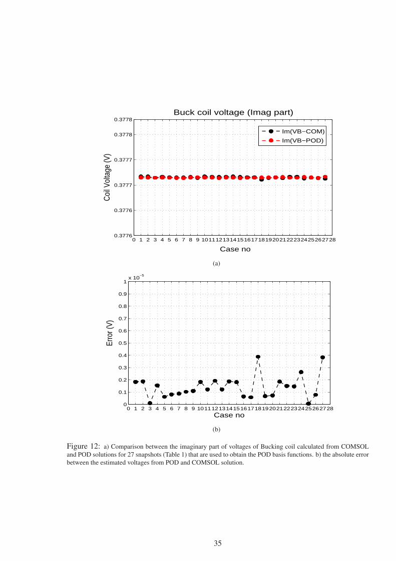
Figures 9 to 12 show real and imaginary parts of voltages of Main and Bucking coils for seencases Table 1 with corresponding error E, which measures the difference between the voltagescalculated using the forward model and the POD solutions. The results look very promising,with a good correlation between voltages calculated using POD and COMSOL solutions. Ascan be seen, for most of the cases the real part of voltages of the Main and Bucking coils can beestimated with an absolute error less than 0.5× 10−4 S/m (for Main coil) and 0.5× 10−6 S/m(for Bucking coil), with the maximum percentage error 6% for both Main and Bucking coils,however larger errors are observed for some cases such as 18 and 27, where most of layers havehigh conductivity (H=1 S/m). The imaginary part of the voltages for both Main and Buckingcoils can be estimated with an absolute error less than 1.5× 10−5 S/m (for Main coil) and3.8× 10−6 S/m (for Bucking coil), with a percentage error less than 1% for both Main andBucking coils.

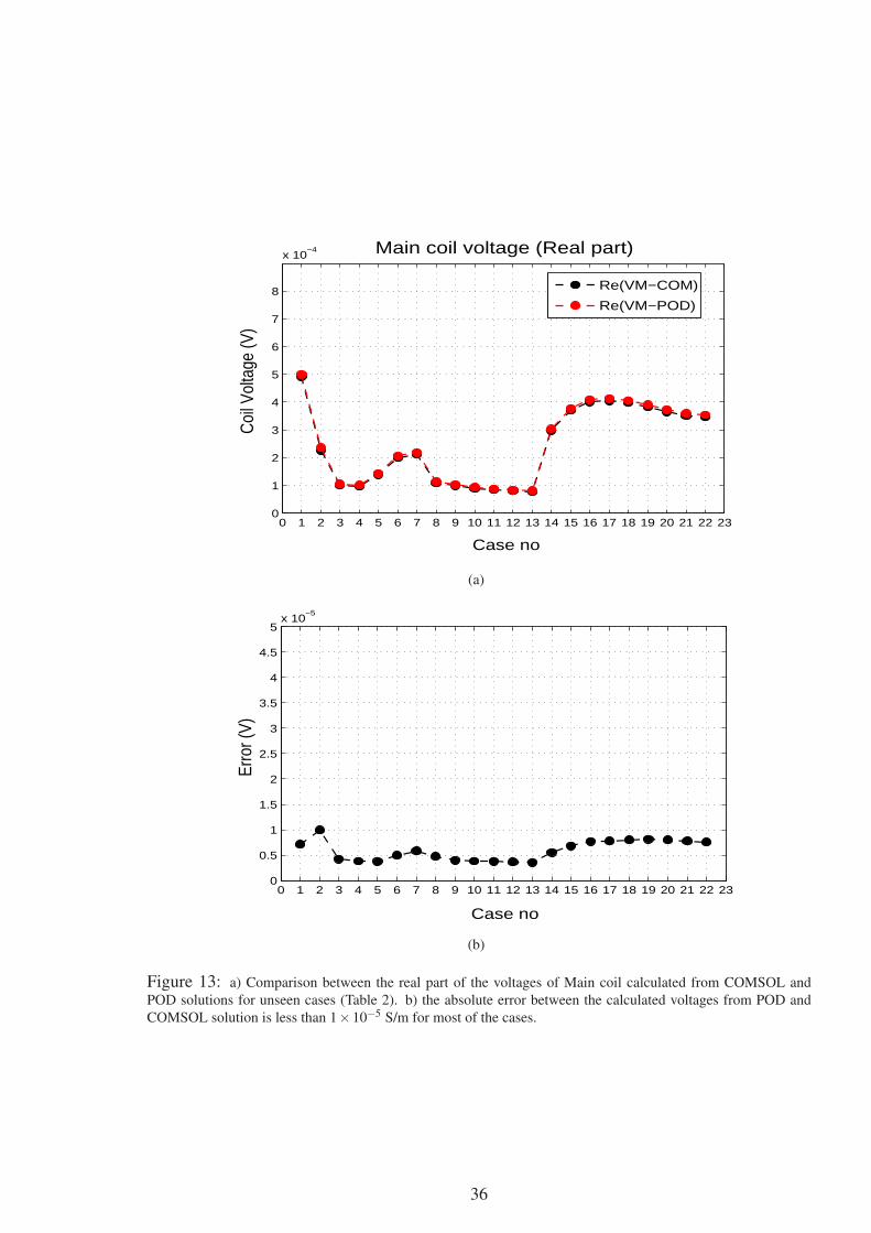
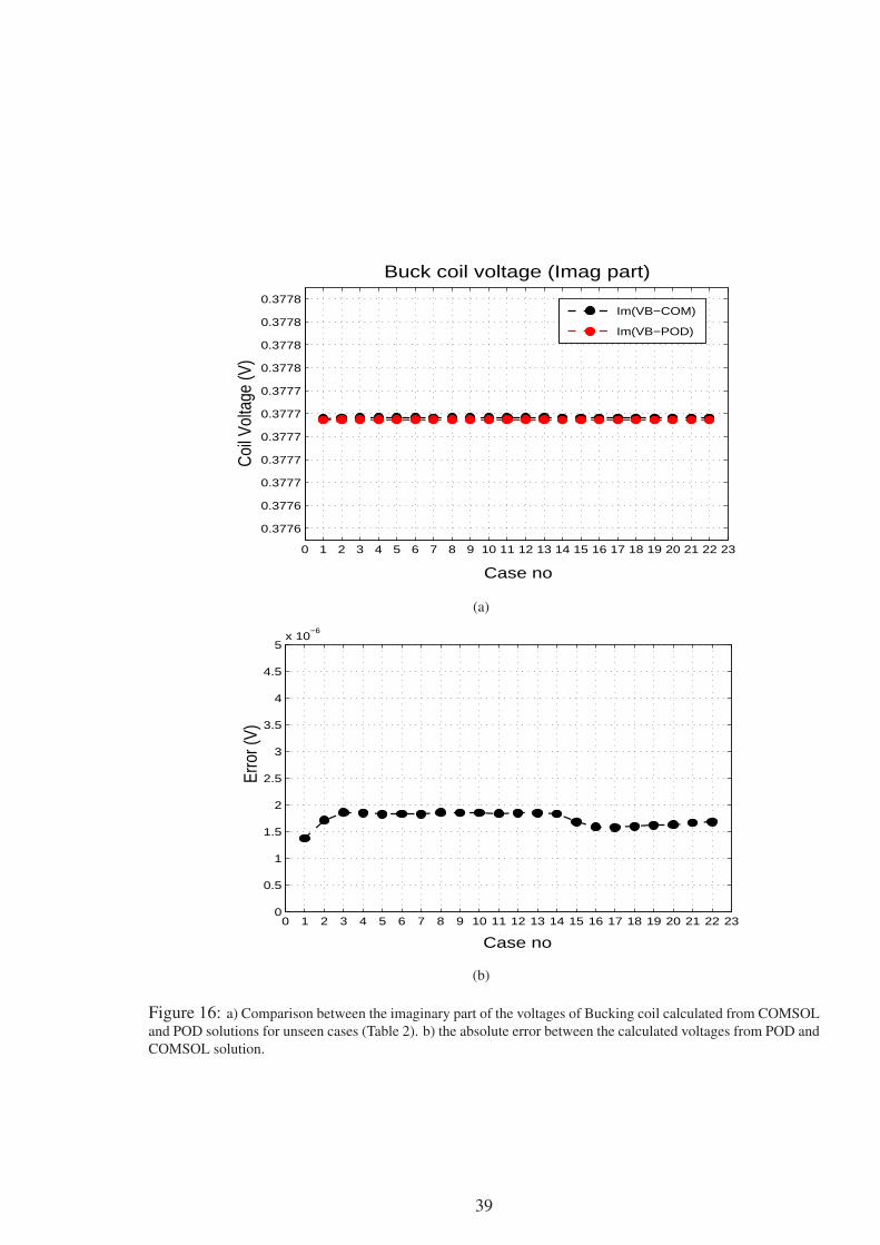
The results of calculated voltages for unseen cases (Table 2) are provided in Figures 13 to16. Good correlation is again found between the calculated voltages from POD and COMSOLsolutions, with absolute difference errors of less than 5×10−6 S/m for the real part and 2×10−6

for the imaginary part of Main and Bucking coils. The voltages of Main and Bucking coils canbe estimated to within a 6% error on real and 1% error on imaginary parts.

5 Conclusions

In this paper, the POD method is introduced as a surrogate model to replace the computationallydemanding COMSOL finite element model that solves Maxwell equations. First, the COMSOLforward model is run to obtain the solution snapshots at different conductivities. The PODbasis functions are then calculated using singular value decomposition. The minimum num-ber of POD basis functions, which can represent the maximum kinetic energy included in thesnapshots, is chosen.

To solve the POD discrete model obtained from the full POD reduced model, a set of sub-matrices independent of conductivity is derived from discretization of the full model. These sub-matrices are then projected onto the reduced space by using the POD basis functions, leadingto a discrete POD model of dimension M which is much smaller than dimension N of the full

15

forward model. In this way, a POD simulation can be run in a few seconds.

The POD model is applied to 27 snapshots obtained from COMSOL using a 5-layer model. Thelayer conductivities are chosen from a combination of three values of conductivities, 0.001 S/m,0.03 S/m and 1 S/m, based on fractional factorial design. The 27 snapshots with 20 POD basisfunctions, for each real and imaginary parts, are chosen to capture more than 99% of the energyof the real part and 99.99% of the energy of the imaginary part.

The results obtained from seen and unseen cases show that the POD solutions agree well withthe ones obtained from the forward model for both real and imaginary parts. Evaluation ofthe accuracy of the POD model is also carried out through the calculation of voltages usingthe POD solutions. The close agreement between voltages estimated from COMSOL and PODsolutions, for both seen and unseen cases, validates the accuracy of POD solutions. Overall, theresults show that the POD method is fast and accurate and thus may be a good candidate forfuture formation conductivity inversion in a layered media.

16

REFERENCES

Anderson, B. and Gianzero, S. (1983). Induction sonde response in stratified media. The LogAnalyst, 24(1):25–31.

Anderson, B. I. (2001). Modeling and Inversion Methods for the Interpretation of ResistivityLogging Tool Response. PhD thesis, Technische Universiteit Delft.

Ardjmandpour, N. (2010). MOdelling and Inversion of Array Induction Tool. PhD thesis,Imperial College London.

Aubry, N., Holmes, P., and Lumley, J. L. (1988). The dynamics of coherent structures in thewall region of a turbulent boundary layer. Journal of Fluid Dynamics, 192:115–173.

Banks, H. T., Joyner, M. L., Wincheski, B., and Winfree, W. P. (2000). Nondestructive evalua-tion using a reduced-order computational methodology. Inverse Problems, 16(4):929–945.

Barber, T., Orban, A., Hazen, G., Long, T., Schlein, R., Alderman, S., Tabanou, J., and Seydoux,J. (1995). A multiarray induction tool optimized for efficient wellsite operation. SPE AnnualTechnical Conference and Exhibition, 22-25 October 1995, Dallas, Texas, SPE 30583.

Barber, T. D., Broussard, T., Minerbo, G. N., Murgatroyd, D., and Sijercic, Z. (1999). In-terpretation of multiarray induction logs in invaded formations at high relative dip angles.40(3):220–217.

Barber, T. D. and Rosthal, R. A. (1991). Using a multiarray induction tool to achieve high-resolution logs with minimum environmental effects. SPE Annual Technical Conference andExhibition, Dallas, Texas.

Bui-Thanh, T., Willcox, K., Ghattas, O., and van Bloemen Waanders, B. (2007). Goal-oriented,model-constrained optimization for reduction of large-scale systems. J. Comput. Phys.,224:880–896.

Cardoso, M. A. and Durlofsky, L. J. (2010). Linearized reduced-order models for subsurfaceflow simulation. J. Comput. Phys., 229(3):681–700.

Chen, X., Navon, I. M., and Fang, F. (2009). A dual-weighted trust-region adaptive POD 4D-VAR applied to a finite-element shallow-water equations model. International Journal forNumerical Methods in Fluids.

Crommelin, D. T. and Majda, A. J. (2004). Strategies for model reduction: Comparing differentoptimal bases. Journal of the Atmospheric Sciences, 61(17):2206–2217.

Daescu, D. N. and Navon, I. M. (2008). A Dual-Weighted approach to order reduction in4DVAR data assimilation. Monthly Weather Review, 136(3):1026–1041.

17

Doll, H. G. (1949). Introduction to induction logging and application to logging of wells drilledwith oil base mud. Journal of Petroleum Technology, 1:148–162.

Dyos, C. J. (1987). Inversion of induction log data by the method of maximum entropy. InSPWLA 28th Annual Logging Symposium Transactions. Society of Professional Well LogAnalysts, July 1-13.

Ellis, D. V. and Singer, J. M. (2007). Well logging for Earth Scientists. Springer, The Nether-lands.

Fang, F., Pain, C. C., Navon, I. M., Gorman, G. J., Piggott, M. D., and Allison, P. A. (2010).The independent set perturbation adjoint method: A new method of differentiating mesh-based fluids models. International Journal for Numerical Methods in Fluids.

Fang, F., Pain, C. C., Navon, I. M., Piggott, M. D., Gorman, G. J., Allison, P. A., and Goddard,A. J. H. (2009). Reduced order modelling of an adaptive mesh ocean model. InternationalJournal for Numerical Methods in Fluids, 59:827–851.

Freedman, R. and Minerbo, G. N. (1991). Maximum Entropy Inversion of Induction-Log Data.SPE Formation Evaluation, 6:259–268.

Fukunaga, K. (1990). ntroduction to Statistical Recognition (2nd edn). Computer Science andScientific Coomputing Series. Academic Press: Boston, MA.

Grove, G. P. and Minerbo, G. N. (1991). An adaptive borehole correction scheme for arrayinduction tools. Society of Professional Well Log Analysts Logging Symposium, Paper P:1–25.

Gunzburger, M. D. (2003). Perspectives in flow control and optimization. SIAM.

Hardman, R. H. and Shen, L. C. (1987). Charts for correcting the effect of formation dip andhole deviation on induction logs. 28(4):349–356.

Holmes, P., Lumley, J. L., and Berkooz, G. (1998). Turbulence Coherent Structures, DynamicalSystems and Symmetry, volume 192.

Hopcroftand, P. O., Gallagher, K., Pain, C. C., and Fang, F. (2009). Three-dimensional sim-ulation and inversion of borehole temperatures for reconstructing past climate in complexsettings. J. Geophys. Res., 114.

Hoteit, I. and Khl, A. (2006). Efficiency of reduced-order, time-dependent adjoint data assimi-lation approaches. Journal of Oceanography, 62:539–550.

Howard, A. Q. (1992). A new invasion model for resistivity log interpretation. Log Analyst,33(2):96–110.

18

Hunka, J., Barber, T. D., Rosthal, R. A., Minerbo, G. N., Head, E. A., Howard, A., Hazen, G.,and Chandler., R. (1990). A new resistivity measurement system for deep formation imag-ing and high-resolution formation evaluation. In Proceedings 1990 SPE Annual TechnicalConference and Exhibition., volume SPE 20559. Society of Petroleum Engineers.

Jolliffe, I. T. (2002). Principal Component Analysis. Springer, second edition.

Karhunen, K. (1946). Zur spektraltheorie stochastischer prozesse. Annales Academi Scien-tiarum Fennic, 34:1–7.

Kirby, M. and Sirovich, L. (1990). Application of the KarhunenLoeve procedure for the charac-terization of human faces. IEEE Transactions on Pattern Analysis and Machine Intelligence,12:103 – 108.

Kosambi, D. D. (1943). Statistics in function space. Journal of the Indian Mathematical Society,7:76 – 88.

Kunisch, K. and Volkwein, S. (2003). Galerkin proper orthogonal decomposition methods fora general equation in fluid dynamics. SIAM Journal on Numerical Analysis, 40(2):492–515.

Lehoucq, R. B., Sorensen, D. C., and Yang, C. (1998). ARPACK Users’ Guide: Solution ofLarge-Scale Eigenvalue Problems with Implicitly Restarted Arnoldi Methods. Siam.

Lin, Y.-Y., Gianzera, S., and Strickland, R. (1984). Inversion of induction logging data using theleast squares technique. In SPWLA 25th Annual Logging Symposium Transactions. Societyof Professional Well Log Analysts, June 10-13.

Loeve, M. (1945). Sur les fonctions aleatoires stationaires du second ordre. Revue Scientifique,83:297–303.

Lumley, J. L. (1967). The structure of inhomogeneous turbulence. Atmospheric Turbulence andWave Propagation, pages 166 – 178.

Luo, Z., Zhu, J., Wang, R., and Navon, I. M. (2007). Proper orthogonal decomposition approachand error estimation of mixed finite element methods for the tropical pacific ocean reducedgravity model. Computer Methods in Applied Mechanics and Engineering, 196(41-44):4184–4195.

Majda, A. J., Timofeyev, I., and Vanden-Eijnden, E. (2003). Systematic strategies for stochasticmode reduction in climate. Journal of the Atmospheric Sciences, 60(14):1705–1722.

Miranda, A., Le Borgne, Y.-A., and Bontempi, G. (2008). New routes from minimal approxi-mation error to principal components. Neural Processing Letters, 27:197–207.

Moran, J. H. (1982). Induction logging-geometrical factors with skin effect. The Log Analyst,23(6):4 – 10.

19

Moran, J. H. and Kunz, K. S. (1962). Basic theory of induction logging and application to studyof two-coil sondes. Geophysics, 27(6):829–858.

Pearson, K. (1901). On lines and planes of closest fit to systems of points in space. 2(6):559572.

Robert, C., Durbiano, S., Blayo, E., Verron, J., Blum, J., and Dimet, F.-X. L. (2005). A reduced-order strategy for 4d-var data assimilation. Journal of Marine Systems, 57(1-2):70 – 82.

Rust, D. and Anderson, B. (1975). An intimate look at induction logging. Technical Reniew 2.

Schilders, W. H. A., van der Vorst, H. A., and Rommes, J. (2008). Model order reduction:theory, research aspects and applications, volume 13. Springer ECMI Series on Mathematicsin Industry.

Thadani, S. G., Merchant, G. A., and Verbout, J. L. (1983). Deconvolution with variable fre-quency induction logging systems. SPWLA Twenty Fourth Annual Logging Symposium, June27-30.

Vauhkonen, M., Kaipio, J. P., Somersalo, E., and Karjalainen, P. A. (1997). Electricalimpedance tomography with basis constraints. Inverse Problems, 13(2):523–530.

Willcox, K., Ghattas, O., van Bloemen Waanders, B., and Bader, B. (2005). An optimizationframework for goal-oriented, model-based reduction of large-scale systems.

Willcox, K. and Peraire, J. (2002). Balanced model reduction via the proper orthogonal decom-position. AIAA Journal, 40:2323 – 2330.

Xiao, J., Geldmacher, I., and Rabinovich, M. (2000). Deviated-well software focusing of mul-tiarray induction measurements. SPWLA 41th Annual Logging Symposium, June 4-7.

Xu, H. (2005). A catalogue of three-level regular fractional factorial designs. Metrika,62(2):259–281.

20

List of Figures

Figure1 Basic two-coil induction tool. The vertical component of the magnetic field from the

transmitter coil induces ground loop currents. The current loops in the conductive formation

produce a secondary magnetic field detected by the receiver coil (Anderson, 2001). . . . . . . 25Figure2 The logging environment such as mud conductivity and borehole size, mud filtrate in-

vasion, adjacent bed and dipping beds affect on the measured signal. To estimate the true

formation conductivity, one needs to correct for these effects. . . . . . . . . . . . . . . . 25Figure3 Layered media to be modelled to generate the required snapshots for POD model re-

duction. We assume that the data are borehole corrected, therefore the borehole is not included

in the model. Layer thickness (layers 1 to 5) is 0.07 m (3 inch). The transmitter coil (Tx) is

situated within layer 2 and Main (RxM) and Bucking (RxB) coils are located 0.15 m (6 inch)

and 0.1 m (4 inch) respectively form Tx. The solution is calculated as the azimuthal component

of magnetic vector potential Aφ, the model imposes the Dirichlet boundary conditions Aφ = 0

on the symmetry axis. . . . . . . . . . . . . . . . . . . . . . . . . . . . . . . . . 26Figure4 Energy percentage captured by POD basis for real and imaginary parts. In our case, we

choose 20 POD basis functions which can capture 99% energy from the real part and 99.99%

energy from the imaginary part. . . . . . . . . . . . . . . . . . . . . . . . . . . . . 27Figure5 Comparison of the real part of azimuthal vector potential between the full model (a) and

the reduced model (b) for a seen case with conductivities of 0.03 (S/m), 0.03 (S/m), 0.001 (S/m),

1 (S/m), 0.001 (S/m) for each layer. c) The error between the forward and POD solution. . . . 28Figure6 Comparison of the imaginary part of azimuthal vector potential between the full model (a)

and the reduced model (b) for a seen case with conductivities of 0.03 (S/m), 0.03 (S/m), 0.001 (S/m),

1 (S/m), 0.001 (S/m) for each layer. c) The error between the forward and POD solution. . . . 29Figure7 Comparison of the real part of azimuthal vector potential between the full model (a)

and the reduced model (b) for an unseen case with conductivities of 0.025 (S/m), 0.033 (S/m),

0.08 (S/m), 0.09 (S/m), 0.09 (S/m) for each layer. c) The error between the forward and POD

solution. . . . . . . . . . . . . . . . . . . . . . . . . . . . . . . . . . . . . . . 30Figure8 Comparison of the imaginary part of azimuthal vector potential between the full model (a)

and the reduced model (b) for an unseen case with conductivities of 0.025 (S/m), 0.033 (S/m),

0.08 (S/m), 0.09 (S/m), 0.09 (S/m) for each layer. c) The error between the forward and POD

solution. . . . . . . . . . . . . . . . . . . . . . . . . . . . . . . . . . . . . . . 31Figure9 a) Comparison between the real part of the voltages of Main coil calculated from COM-

SOL and POD solutions for 27 snapshots (Table 1) that are used to obtain the POD basis func-

tions. b) the absolute error (E = |V mRCOM−V mR

POD|). . . . . . . . . . . . . . . . . . . 32Figure10 a) Comparison between the imaginary part of the voltages of Main coil calculated from

COMSOL and POD solutions for 27 snapshots (Table 1) that are used to obtain the POD basis

functions. b) the absolute error (E = |V mICOM−V mI

POD|). . . . . . . . . . . . . . . . . 33

21

Figure11 a) Comparison between the real part of voltages of Bucking coil calculated from COM-

SOL and POD solutions using equation for 27 snapshots (Table 1) that are used to obtain

the POD basis functions. b) the absolute error between the estimated voltages from POD and

COMSOL solution. . . . . . . . . . . . . . . . . . . . . . . . . . . . . . . . . . 34Figure12 a) Comparison between the imaginary part of voltages of Bucking coil calculated from

COMSOL and POD solutions for 27 snapshots (Table 1) that are used to obtain the POD ba-

sis functions. b) the absolute error between the estimated voltages from POD and COMSOL

solution. . . . . . . . . . . . . . . . . . . . . . . . . . . . . . . . . . . . . . . 35Figure13 a) Comparison between the real part of the voltages of Main coil calculated from COM-

SOL and POD solutions for unseen cases (Table 2). b) the absolute error between the calculated

voltages from POD and COMSOL solution is less than 1×10−5 S/m for most of the cases. . . 36Figure14 a) Comparison between the imaginary part of the voltages of Main coil calculated from

COMSOL and POD solutions for unseen cases (Table 2). b) the absolute error between the

calculated voltages from POD and COMSOL solution. . . . . . . . . . . . . . . . . . . 37Figure15 a) Comparison between the real part of the voltages of Bucking coil calculated from

COMSOL and POD solutions for unseen cases (Table 2). b) the absolute error between the

calculated voltages from POD and COMSOL solution. . . . . . . . . . . . . . . . . . . 38Figure16 a) Comparison between the imaginary part of the voltages of Bucking coil calculated

from COMSOL and POD solutions for unseen cases (Table 2). b) the absolute error between

the calculated voltages from POD and COMSOL solution. . . . . . . . . . . . . . . . . 39

22

No of Cases Layer 1 Layer 2 Layer3 Layer 4 Layer 5

1 0.001 0.001 0.001 0.001 0.0012 0.001 0.001 0.03 0.03 0.0013 0.001 0.001 1 1 0.0014 0.001 0.03 0.001 0.03 15 0.001 0.03 0.03 1 16 0.001 0.03 1 0.001 17 0.001 1 0.001 1 0.038 0.001 1 0.03 0.001 0.039 0.001 1 1 0.03 0.03

10 0.03 0.001 0.001 0.03 0.0311 0.03 0.001 0.03 1 0.0312 0.03 0.001 1 0.001 0.0313 0.03 0.03 0.001 1 0.00114 0.03 0.03 0.03 0.001 0.00115 0.03 0.03 1 0.03 0.00116 0.03 1 1 0.001 117 0.03 1 0.03 0.03 118 0.03 1 1 1 119 1 0.001 0.001 1 120 1 0.001 0.03 0.001 121 1 0.001 1 0.03 122 1 0.03 0.001 1 0.0323 1 0.03 1 0.03 0.0324 1 0.03 1 1 0.0325 1 1 0.001 0.03 0.00126 1 1 1 1 0.00127 1 1 0.001 0.001 0.001

Table 1: The 27 best runs of 3 values of conductivities (0.001 S/m, 0.03 S/m and 1 S/m) for 5 layers determinedbased on the fractional factorial design (Xu, 2005).

23

No of Cases Layer 1 Layer 2 Layer3 Layer 4 Layer 5

1 0.25 0.25 0.25 0.25 0.252 0.25 0.22 0.05 0.025 0.0253 0.05 0.025 0.025 0.025 0.0254 0.025 0.025 0.025 0.025 0.0255 0.025 0.025 0.03 0.08 0.096 0.03 0.08 0.09 0.09 0.097 0.09 0.09 0.09 0.09 0.098 0.08 0.03 0.025 0.025 0.0259 0.03 0.025 0.025 0.025 0.025

10 0.025 0.025 0.025 0.015 0.01411 0.025 0.023 0.015 0.014 0.01412 0.023 0.015 0.014 0.014 0.01413 0.015 0.014 0.014 0.014 0.01414 0.014 0.03 0.17 0.2 0.215 0.03 0.17 0.2 0.2 0.216 0.017 0.2 0.2 0.2 0.217 0.2 0.2 0.2 0.2 0.218 0.2 0.2 0.2 0.19 0.1719 0.2 0.2 0.19 0.17 0.1620 0.2 0.19 0.17 0.16 0.1621 0.19 0.17 0.16 0.16 0.1622 0.17 0.16 0.16 0.16 0.16

Table 2: The conductivity of the each layer for unseen cases.

24

Figure 1: Basic two-coil induction tool. The vertical component of the magnetic field from the transmitter coilinduces ground loop currents. The current loops in the conductive formation produce a secondary magnetic fielddetected by the receiver coil (Anderson, 2001).

Figure 2: The logging environment such as mud conductivity and borehole size, mud filtrate invasion, adjacentbed and dipping beds affect on the measured signal. To estimate the true formation conductivity, one needs tocorrect for these effects.

25

(a)

Figure 3: Layered media to be modelled to generate the required snapshots for POD model reduction. We assumethat the data are borehole corrected, therefore the borehole is not included in the model. Layer thickness (layers 1 to5) is 0.07 m (3 inch). The transmitter coil (Tx) is situated within layer 2 and Main (RxM) and Bucking (RxB) coilsare located 0.15 m (6 inch) and 0.1 m (4 inch) respectively form Tx. The solution is calculated as the azimuthalcomponent of magnetic vector potential Aφ, the model imposes the Dirichlet boundary conditions Aφ = 0 on thesymmetry axis.

26

0 1 2 3 4 5 6 7 8 9 10 11 12 13 14 15 16 17 18 19 20 21 22 23 24 25 26 27 28

Number of POD bases

50

60

70

80

90

100

Cap

ture

d En

ergy

(%)

Real partImaginary part

(a)

Figure 4: Energy percentage captured by POD basis for real and imaginary parts. In our case, we choose 20 PODbasis functions which can capture 99% energy from the real part and 99.99% energy from the imaginary part.

27

(a) COMSOL solution

(b) POD solution

(c) Error

Figure 5: Comparison of the real part of azimuthal vector potential between the full model (a) and the reducedmodel (b) for a seen case with conductivities of 0.03 (S/m), 0.03 (S/m), 0.001 (S/m), 1 (S/m), 0.001 (S/m) for eachlayer. c) The error between the forward and POD solution.

28

(a) COMSOL solution

(b) POD solution

(c) Error

Figure 6: Comparison of the imaginary part of azimuthal vector potential between the full model (a) and thereduced model (b) for a seen case with conductivities of 0.03 (S/m), 0.03 (S/m), 0.001 (S/m), 1 (S/m), 0.001 (S/m)for each layer. c) The error between the forward and POD solution.

29

(a) COMSOL solution

(b) POD solution

(c) Error

Figure 7: Comparison of the real part of azimuthal vector potential between the full model (a) and the reducedmodel (b) for an unseen case with conductivities of 0.025 (S/m), 0.033 (S/m), 0.08 (S/m), 0.09 (S/m), 0.09 (S/m)for each layer. c) The error between the forward and POD solution.

30

(a) COMSOL solution

(b) POD solution

(c) Error

Figure 8: Comparison of the imaginary part of azimuthal vector potential between the full model (a) and thereduced model (b) for an unseen case with conductivities of 0.025 (S/m), 0.033 (S/m), 0.08 (S/m), 0.09 (S/m),0.09 (S/m) for each layer. c) The error between the forward and POD solution.

31

0 1 2 3 4 5 6 7 8 9 101112131415161718192021222324252627280

1

2

3

4x 10

−3 Main coil voltage (Real part)

Case no

Coi

l Vol

tage

(V)

Re(VM−COM)

Re(VM−POD)

(a)

0 1 2 3 4 5 6 7 8 9 101112131415161718192021222324252627280

1

2

3

4

5x 10

−4

Case no

Erro

r (V)

(b)

Figure 9: a) Comparison between the real part of the voltages of Main coil calculated from COMSOL andPOD solutions for 27 snapshots (Table 1) that are used to obtain the POD basis functions. b) the absolute error(E = |V mR

COM−V mRPOD|).

32

0 1 2 3 4 5 6 7 8 9 101112131415161718192021222324252627280.3912

0.3913

0.3914

0.3915Main coil voltage (Imag part)

Case no

Coi

l Vol

tage

(V)

Im(VM−COM)

Im(VM−POD)

(a)

0 1 2 3 4 5 6 7 8 9 101112131415161718192021222324252627280

0.5

1

1.5

2

2.5

3

3.5

4

4.5

5x 10

−5

Case no

Erro

r (V)

(b)

Figure 10: a) Comparison between the imaginary part of the voltages of Main coil calculated from COMSOLand POD solutions for 27 snapshots (Table 1) that are used to obtain the POD basis functions. b) the absolute error(E = |V mI

COM−V mIPOD|).

33

0 1 2 3 4 5 6 7 8 9 101112131415161718192021222324252627280

0.2

0.4

0.6

0.8

1

1.2

1.4

1.6

1.8

2x 10

−3 Buck coil voltage (Real part)

Case no

Coi

l Vol

tage

(V)

Re(VB−COM)

Re(VB−POD)

(a)

0 1 2 3 4 5 6 7 8 9 101112131415161718192021222324252627280

1

2

x 10−4

Case no

Erro

r (V)

(b)

Figure 11: a) Comparison between the real part of voltages of Bucking coil calculated from COMSOL and PODsolutions using equation for 27 snapshots (Table 1) that are used to obtain the POD basis functions. b) the absoluteerror between the estimated voltages from POD and COMSOL solution.

34

0 1 2 3 4 5 6 7 8 9 101112131415161718192021222324252627280.3776

0.3776

0.3777

0.3777

0.3778

0.3778Buck coil voltage (Imag part)

Case no

Coi

l Vol

tage

(V)

Im(VB−COM)

Im(VB−POD)

(a)

0 1 2 3 4 5 6 7 8 9 101112131415161718192021222324252627280

0.1

0.2

0.3

0.4

0.5

0.6

0.7

0.8

0.9

1x 10

−5

Case no

Erro

r (V)

(b)

Figure 12: a) Comparison between the imaginary part of voltages of Bucking coil calculated from COMSOLand POD solutions for 27 snapshots (Table 1) that are used to obtain the POD basis functions. b) the absolute errorbetween the estimated voltages from POD and COMSOL solution.

35

0 1 2 3 4 5 6 7 8 9 10 11 12 13 14 15 16 17 18 19 20 21 22 230

1

2

3

4

5

6

7

8

x 10−4 Main coil voltage (Real part)

Case no

Coi

l Vol

tage

(V)

Re(VM−COM)

Re(VM−POD)

(a)

0 1 2 3 4 5 6 7 8 9 10 11 12 13 14 15 16 17 18 19 20 21 22 230

0.5

1

1.5

2

2.5

3

3.5

4

4.5

5x 10

−5

Case no

Erro

r (V)

(b)

Figure 13: a) Comparison between the real part of the voltages of Main coil calculated from COMSOL andPOD solutions for unseen cases (Table 2). b) the absolute error between the calculated voltages from POD andCOMSOL solution is less than 1×10−5 S/m for most of the cases.

36

0 1 2 3 4 5 6 7 8 9 10 11 12 13 14 15 16 17 18 19 20 21 22 230.3913

0.3913

0.3914

0.3914

0.3914

0.3914Main coil voltage (Imag part)

Case no

Coi

l Vol

tage

(V)

Im(VM−COM)

Im(VM−POD)

(a)

0 1 2 3 4 5 6 7 8 9 10 11 12 13 14 15 16 17 18 19 20 21 22 230

0.5

1

1.5

2

2.5

3

3.5

4

4.5

5x 10

−6

Case no

Erro

r (V)

(b)

Figure 14: a) Comparison between the imaginary part of the voltages of Main coil calculated from COMSOLand POD solutions for unseen cases (Table 2). b) the absolute error between the calculated voltages from POD andCOMSOL solution.

37

0 1 2 3 4 5 6 7 8 9 10 11 12 13 14 15 16 17 18 19 20 21 22 230

0.5

1

1.5

2

2.5

3

3.5

4

4.5

5x 10

−4 Buck coil voltage (Real part)

Case no

Coi

l Vol

tage

(V)

Re(VB−COM)

Re(VB−POD)

(a)

0 1 2 3 4 5 6 7 8 9 10 11 12 13 14 15 16 17 18 19 20 21 22 230

0.1

0.2

0.3

0.4

0.5

0.6

0.7

0.8

0.9

1x 10

−5

Case no

Erro

r (V)

(b)

Figure 15: a) Comparison between the real part of the voltages of Bucking coil calculated from COMSOL andPOD solutions for unseen cases (Table 2). b) the absolute error between the calculated voltages from POD andCOMSOL solution.

38

0 1 2 3 4 5 6 7 8 9 10 11 12 13 14 15 16 17 18 19 20 21 22 23

0.3776

0.3776

0.3777

0.3777

0.3777

0.3777

0.3777

0.3778

0.3778

0.3778

0.3778

Buck coil voltage (Imag part)

Case no

Coi

l Vol

tage

(V)

Im(VB−COM)

Im(VB−POD)

(a)

0 1 2 3 4 5 6 7 8 9 10 11 12 13 14 15 16 17 18 19 20 21 22 230

0.5

1

1.5

2

2.5

3

3.5

4

4.5

5x 10

−6

Case no

Erro

r (V)

(b)

Figure 16: a) Comparison between the imaginary part of the voltages of Bucking coil calculated from COMSOLand POD solutions for unseen cases (Table 2). b) the absolute error between the calculated voltages from POD andCOMSOL solution.

39