Clemson UniversityTigerPrints

All Dissertations Dissertations

12-2015

Soviet Launch of Sputnik: Sputnik-InspiredEducational Reform and Changes in PrivateReturns in AmericaHyeonggu ChaClemson University, hcha@g.clemson.edu

Follow this and additional works at: https://tigerprints.clemson.edu/all_dissertations

Part of the Public Policy Commons

This Dissertation is brought to you for free and open access by the Dissertations at TigerPrints. It has been accepted for inclusion in All Dissertations byan authorized administrator of TigerPrints. For more information, please contact kokeefe@clemson.edu.

Recommended CitationCha, Hyeonggu, "Soviet Launch of Sputnik: Sputnik-Inspired Educational Reform and Changes in Private Returns in America"(2015). All Dissertations. 1550.https://tigerprints.clemson.edu/all_dissertations/1550

SOVIET LAUNCH OF SPUTNIK: SPUTNIK-INSPIRED EDUCATIONAL REFORM

AND CHANGES IN PRIVATE RETURNS IN AMERICA

A Dissertation

Presented to

the Graduate School of

Clemson University

In Partial Fulfillment

of the Requirements for the Degree

Doctor of Philosophy

Policy Studies

by

Hyeonggu Cha

December 2015

Accepted by:

Dr. Curtis Simon, Committee Chair

Dr. Robert Tollison

Dr. Holley Ulbrich

Dr. Joseph Stewart

ii

ABSTRACT

On October 4th 1957, the Soviet Union launched the world’s first man-made satellite,

Sputnik 1, into an elliptical low Earth orbit. This surprise triggered an arms race between

the United States and the Soviet Union, as well as science-oriented educational reform in

the U.S. Sputnik sparked changes for the U.S. in military, politics, policies, and

education. The launch of Sputnik woke Americans up from complacency came from

technology, science, and educational superiority. Educational reform started with

emphasizing science and defense education and it was expanded to all levels of

education. Early reforms, the National Science Foundation (NSF), and the National

Defense Education Act (NDEA) of 1958 were focused on science and defense education

during Eisenhower’s administration. Domestic programs such as Civil Rights and Great

Society diffused educational policy to produce more general human capitals for improve

poverty and economic growth during the administrations of Kennedy and Johnson. The

Higher Education Act (HEA) of 1965 was enacted to support postsecondary education. I

assert that these policy outputs have contributed to the dramatic increase in the supply of

college graduates since 1960. This study begins with emphasizing the Soviet launching of

Sputnik and educational reform in early 1960s in U.S. as a cause and effect relationship.

Analysis focuses on the policy process of educational reform by applying Kingdon’s

multiple streams model, and on the economic effects of increase in the supply of college

graduates by applying Acemoglu’s theory, the pooling and separating equilibria (1999).

According to Acemoglu, economy transitions from initial pooling equilibrium to

separating equilibrium as supply of high skilled labor increases and thus labor markets

iii

show different patterns in unemployment rates and wage structures for skilled and

unskilled, as well as job mismatch. I find that occupational segregation at the state labor

markets increases corresponding to supply of college graduates, and overeducation

decreases as occupational segregation increases. Moreover, occupational segregation has

positive wage effects and wage penalty from overeducation becomes smaller in states

where occupations are more separated between the skilled and the unskilled. College

graduates earn more wage premiums in states where occupations are more separated

between the skilled and the unskilled.

iv

DEDICATION

To my father & mother: I thank God for allowing us to have so much time

together. Thanks for your endurance and support of this rotten kid. I wish medical

technology can soon give hope to my father and other people who are suffering from

Parkinson’s disease.

v

ACKNOWLEDGMENTS

Thanks to Dr. Robert Tollison. Since when I was in the Economics Department, I

have taken all of your classes and you always encouraged me and other students in your

class, and gave me your helpful hands generously and freely whenever I needed help.

Thanks to Dr. Holley Ulbrich for your precious feedbacks and comments for improving

this paper. I really enjoyed conversations with you in your classes. When I needed to talk

to someone, you were there and listened to me. Thanks to Dr. Joseph Stewart your

willingness to serve on the committee and all of your precious feedbacks and

recommendations. Thanks to Dr. Frankie Felder and Dr. Christopher Ruth for all of your

aid in helping me to graduate this semester. You two gave me hope when I felt low.

Thanks to my friend Ahmed and his wife Omnia for your concerns and encouragements

when I went through difficult times. Thanks to Virginia Caswell and Mack Caswell for

your concern for me always. Thanks to my friend Dean Krupp and his family. If I did not

know Jesus Christ, we would have not known each other. Thanks for the long time you

were there as a friend. Without your help, I would not have finished this dissertation.

I am especially grateful to Dr. Curtis Simon: “It is not the healthy who need a

doctor, but the sick” (Luke 5:31). When I was a weed in the field, you taught me and

made me a useful human capital. Only a good teacher can turn a weed into an effective

human capital.

I am sinning God with gratitude in my heart. To God be the glory, for He has

done glorious things.

vi

TABLE OF CONTENTS

Page

TITLE PAGE .................................................................................................................... i

ABSTRACT ..................................................................................................................... ii

DEDICATION and ACKNOWLEDGMENTS .............................................................. iii

LIST OF TABLES ........................................................................................................ viii

LIST OF FIGURES ........................................................................................................ ix

CHAPTER

I. Introduction .................................................................................................... 1

II. Literature Review........................................................................................... 9

1. Change in Wage Structure ................................................................... 9

2. Theory about Existence of Overeducation ......................................... 12

3. Overeducation: Permanent or Transitory? ......................................... 13

4. Measurement of Required Education................................................. 15

5. Duncan-Hoffman and Verdugo-Verdugo .......................................... 16

6. Job Mismatch and Productivity ......................................................... 18

7. Quantile Regression ........................................................................... 19

8. Unobserved Heterogeneity................................................................. 20

III. Hypothetical Framework ............................................................................. 23

1. Arms Race Model .............................................................................. 24

1-1. Richardson’s Arms Race Model .............................................. 25

1-2. Prisoner’s Dilemma Game....................................................... 26

1-3. Competitive Arms Accumulation Model ................................ 27

2. Agenda Setting .................................................................................... 29

2-1. Problem Stream ....................................................................... 30

2-2. Policy Stream ........................................................................... 34

2-3. Politics Stream ......................................................................... 37

vii

Table of Contents (Continued) Page

IV. Equality of Opportunity ............................................................................... 42

1. Paternalism ......................................................................................... 42

2. Public Choice ..................................................................................... 45

3. Expansion of Reform ......................................................................... 47

V. Policy Outputs and College Enrollments ..................................................... 52

1. National Science Foundation (NSF) .................................................. 52

2. National Defense Educational Act (NDEA) of 1958 ......................... 54

3. Higher Education Act (HEA) of 1965 ............................................... 56

4. College Enrollments........................................................................... 57

5. Sputnik-induced Federalism in American Educational System ......... 66

VI. Empirical Study ........................................................................................... 72

1. Summary Statistics............................................................................. 75

2. Empirical Specification ...................................................................... 88

3. Results ................................................................................................ 90

3-1. Wage Effects of Industry-Occupational Segregation .................

and Mismatch ......................................................................... 90

3-2. College Wage Premiums ...................................................... 106

VII. Conclusion ................................................................................................... 116

REFERENCES ............................................................................................................ 120

viii

LIST OF TABLES

Table Page

Table 1: Years of Overeducation and Incidence of Mismatch ....................................... 6

Table 2: The Arms Race as a Prisoner’s Dilemma Game ............................................. 27

Table 3: Average Amount ($) of Federal Financial Aid Awarded to Full-time,

Full-Year Undergraduates by Race ........................................................ 65

Table 4: Summary Statistics .......................................................................................... 75

Table 5: Duncan-Hoffman Overeducation by Occupations, 2000................................. 85

Table 6: Duncan-Hoffman Undereducation by Occupations, 2000 ............................... 86

Table 7: Specification (1) for Wage Effects of Industry-Occupational Segregation ..... 92

Table 8: Specification (2) for Wage Effects of Industry-Occupational Segregation ..... 94

A. Duncan-Hoffman Mismatch ......................................................................... 94

B. Verdugo-Verdugo Mismatch......................................................................... 95

Table 9: Specification (3) for Wage Effects of Industry-Occupational Segregation ..... 98

A. Duncan-Hoffman Mismatch ......................................................................... 98

B. Verdugo-Verdugo Mismatch......................................................................... 99

Table 10: Alternative Specification

for Wage Effects of Industry-Occupational Segregation ...................... 104

Table 11: Specification (1) for College Wage Premiums ............................................ 108

Table 12: Specification (2) for College Wage Premiums ............................................ 110

A. Duncan-Hoffman Mismatch ..................................................................... 110

B. Verdugo-Verdugo Mismatch..................................................................... 111

Table 13: Specification (3) for College Wage Premiums ............................................ 113

A. Duncan-Hoffman Mismatch ..................................................................... 113

B. Verdugo-Verdugo Mismatch..................................................................... 114

ix

LIST OF FIGURES

Figure Page

Figure 1: Wonder Why We are Not Keeping Pace? ................................................. 3

Figure 2: College/High School Wage Ratio ........................................................... 10

Figure 3: Hypothetical Framework ......................................................................... 23

Figure 4: Military Expenditure Reaction Functions ............................................... 26

Figure 5: College Enrollments of Recent High School Completers, 16-24 Old ..... 58

Figure 6: Total Fall Enrollment by Sex ................................................................ 59

Figure 7: College Enrollment of Recent High School Completers,

By Income Level ............................................................................. 59

Figure 8: College Enrollment of Recent High School Completers by Race........... 60

Figure 9: Total Fall Enrollment by Age ................................................................. 61

Figure 10: Bachelor’s Degree Conferred by Field of Study ................................... 62

Figure 11: Tuition and Required Fees ($2012-2013 Constant dollars) ................. 63

Figure 12: Percentage of Undergraduates Receiving

Federal Financial Aid by Race ...................................................... 64

Figure 13: Federal R&D Outlays, 1949-2005 ($2000FY) ...................................... 68

Figure 14: Expenditure for Education by Federal Government.............................. 69

Figure 15: Expenditure for Higher Education 1962-2008 ..................................... 70

Figure 16: Concept of Occupational Segregation by Skill Groups ......................... 73

Figure 17: Segregation Index vs. Population of College and More Educated

By State of Residence, 2000 ......................................................... 79

Figure 18: Segregation Index by State (%), 2000 ................................................... 81

x

List of Figures (Continued)

Figure Page

Figure 19: Overeducation vs. Segregation Index by State of Residence, 2000 ...... 82

A. Duncan-Hoffman Overeducation .................................................. 82

B. Verdugo-Verdugo Overeducation ................................................. 83

Figure 20: Overeducation vs. College Population by State of Residence, 2000 .... 84

A. Duncan-Hoffman Overeducation .................................................. 84

B. Verdugo-Verdugo Overeducation ................................................. 84

CHAPTER ONE

INTRODUCTION

This paper analyzes educational reform in the early 1960s in the United States, and

its economic consequences. This paper is consisted of two parts: the first part analyzes

policy process of educational reform in early 1960s in the U.S., and the second part

analyzes its economic consequences over time from 1960 to 2000. Instead of focusing on

a single specific policy, I focus on a policy event, which is the educational reform.

Sometimes reform movements in a society arise domestically, but sometimes they

happens by exogenous event. My observation is that the education reform in the early

1960s in America did not arise domestically but was triggered by an exogenous event,

which was the Soviet launch of Sputnik, on October 4, 1957. Therefore, I treat the launch

of Sputnik as a cause of the policy event.

According to the National Aeronautics and Space Act (NASA), Sputnik was the

world’s first artificial satellite and took about 98 minutes to orbit the Earth on its

elliptical path1. I begin this paper with the claim that there is a cause and effect

relationship between the Soviet launching of Sputnik and educational reform in the

United States. My observation is that there were immediate responses from the American

government such as: (1) U.S. Congress increased the National Science Foundation (NSF)

appropriation to $136 million for the 12 months beginning July 1, 1958 for existing NSF

educational programs and for the initiation of new ones. In 1960, the NSF’s appropriation

1 http://history.nasa.gov/sputnik/

2

was $152.7 million and 2000 grants were made. (2) President Eisenhower signed the

National Defense Education Act (NDEA) into law in September 1958. The NDEA

poured $887 million over four years into programs intended to develop talented people in

America in fields related to national defense, and in 1965, Congress passed the Higher

Education Act (HEA) to assist postsecondary education.

The reason why I claim that Sputnik triggered educational reform in America

rather than other countries is that during the Cold War, the Soviet Union and America

(two superpowers) were in an arms race in developing the Inter Continental Ballistic

Missile (ICBM), nuclear weapons, and so on. Moreover, in 1955, America also had

established a project to launch its own satellite, which was called Vanguard. The Project

Vanguard was a program managed by the United States Naval Research Laboratory

(NRL), which intended to launch the first artificial satellite into Earth orbit using a

Vanguard rocket as the launch vehicle. Therefore, the two superpowers were not only in

arms race in missiles and nuclear weapons, but also in launching satellites, a competition

known as the space race2. In this competitive mood, the Soviet launch of Sputnik 1

brought a sudden change in the image of America, which had previously believed itself to

be the superior in education, science, technology, and military power in the world.

2 It is called the space race to distinguish from a formal arms race because its domain is the exterior of the

earth. In this paper, however, I consider the space race as an arms race in satellites such as arms race in

missiles or arms race in nuclear weapons, rather than separating space race from arms race as a different

concept.

3

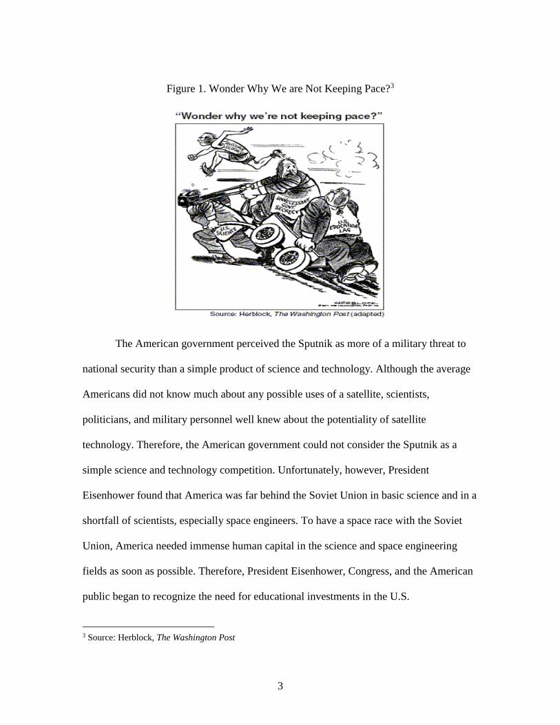
Figure 1. Wonder Why We are Not Keeping Pace?3

The American government perceived the Sputnik as more of a military threat to

national security than a simple product of science and technology. Although the average

Americans did not know much about any possible uses of a satellite, scientists,

politicians, and military personnel well knew about the potentiality of satellite

technology. Therefore, the American government could not consider the Sputnik as a

simple science and technology competition. Unfortunately, however, President

Eisenhower found that America was far behind the Soviet Union in basic science and in a

shortfall of scientists, especially space engineers. To have a space race with the Soviet

Union, America needed immense human capital in the science and space engineering

fields as soon as possible. Therefore, President Eisenhower, Congress, and the American

public began to recognize the need for educational investments in the U.S.

3 Source: Herblock, The Washington Post

4

The second part of this paper is about the economic analysis of consequences of

educational reform. I observe that, since 1960, there has been an increase in college

enrollments. In 1940, less than one American adult in twenty (4.6 percent) was a college

graduate, but the number had quadrupled to one in five (19.4percent) in 1986 (Orfield,

1990). College enrollment was up 45 percent between 1970 and 1983 (Orfield, 1990). In

the beginning of the educational reform, the purpose of the NSF was educating science

elites. The purpose of the NDEA (1958) became a little bit broader focusing on science,

technology, engineering, and mathematics. Later, HEA (1965) was purposed to provide

financial support for general postsecondary education, and was reauthorized many times

up to 2013. Although NSF and NDEA (1958) produced science-related human capitals

intensively, with the perspective of higher education policy, I observe that sequential

education related policies have contributed to an increase in the supply of college

graduates in the labor market. Therefore, I argue that the consequences of the continuous

educational reforms is an increase in the supply of college graduates in the U.S. labor

market.

Some scholars argue that the wage rate of college graduates relative to the high

school graduates, called college wage premium, has been decreased due to an oversupply

of college graduates. For example, Freeman (1975) was the first observant of wage

depression for college graduates. He observed deterioration of economic position of

college graduates between 1969 and 1973, and claimed that there was over investments in

college education in the United States.

5

Autor et al. (1998), however, found that widespread skill-biased technological

changes (SBTC) in the 1980s brought a huge demand for highly educated workers, as

well as a change in wage structure. He used usage of a computer as a proxy measurement

of SBTC and asserted that computer-led industrialization increased demands for skilled

labor and highly educated workers. Therefore, he claimed that over time, relative wages

of college graduates to high school graduates has been increased.

Acemoglu (1999) uses pooling and separating equilibria to explain wage

inequality in 1980s U.S. According to him, when skilled workers are few in the labor

market and productivity gap is small between skilled and unskilled, firms create middling

jobs for both skilled and unskilled workers because creating jobs separately for skilled

and unskilled is not profitable. When skilled workers are abundant in the labor market,

firms create jobs separately for the skilled and the unskilled. By this theory, the economy

transforms from the pooling equilibrium to the separating equilibrium. In separating

equilibrium, wages for skilled workers are much higher but wages for unskilled workers

are much lower than in the pooling equilibrium. Unemployment rates become higher for

both the skilled and the unskilled because firms increase job screening to find better

matched workers, but job mismatch becomes lower.

6

Table 1. Years of Overeducation and Incidence of Mismatch

Years of Overeducation for Total Incidence of Mismatch for College Graduates (%)

Mean Variance Obs. Required Over Under Obs.

1960 0.58 1.36 166301 30.40 62.27 7.33 10056

1970 0.53 1.30 182258 27.86 68.67 3.47 11552

1980 0.78 1.47 1067092 28.43 68.33 3.24 116681

1990 0.62 1.18 1370669 54.04 42.94 3.02 216396

2000 0.59 1.13 1583545 62.68 34.66 2.66 288056

Table 1 shows years of overeducation for the total sample and the incidence of

mismatch for college graduates, respectively.4 Years of overeducation is measured based

on the Duncan-Hoffman mismatch measurement, which is actual education minus mode

years of education in each occupation.5 Years of overeducation measures how many

years of education are surplus over the education that the occupation requires. The left

hand side of the table reveals that, since 1980, the mean value of years of overeducation

has decreased and variance has been smaller. The right hand side of the table is made

based on mismatch dummy variables. For example, required education is a dummy

variable equal to 1 if the worker’s educational attainment is equal to the mode year of

education in each occupation. Overeducation is equal to 1 if his or her education is more

than mode year of education, and undereducation is equal to 1 if his or her education is

4 Generally, economic concern of job mismatch is on overeducation because overeducated workers earn less

than their marginal product, and overeducation is the challenge for mainly college graduates than high school

graduates. 5 Methodology is explained in the literature review.

7

less than mode year of education. It shows that, since 1970, the percentage of college

graduates categorized to required education has been increased, and overeducation has

been decreased.

In this paper, I examine the economic effects of the increase in supply of college

graduates by applying Acemoglu’s theory, the pooling and separating equilibria, in three

aspects: wage effects of industry-occupational segregation, job mismatch, and college

wage premium. I differentiate this paper from previous literatures in two ways. First, with

applying Acemoglu’s theory, I focus on the event of educational reform in America and

thereby I link educational reform and increase in the supply of college graduates.

Therefore, in this paper, supply of college graduates is not an exogenous variable.

Second, with regard to job mismatch, previous literature has not considered the transition

of the economy. Applying Acemoglu’s theory, I measure wage effects of mismatch in the

relation with transition of economy from the pooling equilibrium to the separating

equilibrium. In other words, the magnitudes of wage penalty related with overeducation

may be different in the pooling equilibrium and in the separating equilibrium as wages

for skilled worker are expected to be different from different equilibria.

The outline of the paper is as follows. Chapter 2 reviews previous literature about

changes in wage structure in America and job mismatch. In Chapter 3, I propose three

arms race models to explain the relationship between Sputnik and educational reform. By

applying Kingdon’s multiple streams I try to understand the policy process of policy

outputs in the beginning of the educational reform. In Chapter 4, I review the government

financial aid for education with different views. In Chapter 5, I describe policy outputs

8

such as National Science Foundation (NSF), National Defense Educational Act of 1958,

and Higher Education Act of 1965, and trend of college enrollments as policy effects.

Chapter 6 reports results of the empirical study, and summary and conclusion remarks are

in Chapter 7.

9

CHAPTER TWO

LITERATURE REVIEW

1. Change in Wage Structure

Slonimczyk (2013) shows that skill mismatch was a significant source of

inequality in real earnings in the U.S. during 1973-2002. He uses the Duncan-Hoffman

mismatch measure. His inequality measurements are the variance of log earnings, the

Gini coefficient, and percentile gaps of earnings by using General Education

Development (GED), Dictionary of Occupational Titles (DOT) to measure required

education, and using data from CPS 1973 to 2002. Over-education rates for males and

females were around 15% in 1973 and increasing constantly throughout the period to

reach levels of around 35% of the employed labor force, while under-education follows a

downward trend. Surplus and deficit qualifications taken together account for 4.3% and

4.6% of the variance of log earnings (around 15% of the total explained variance in 2002)

for males and females, respectively.

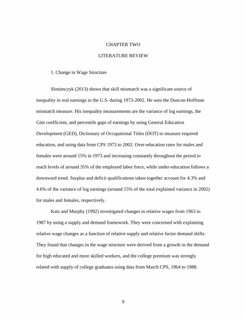
Katz and Murphy (1992) investigated changes in relative wages from 1963 to

1987 by using a supply and demand framework. They were concerned with explaining

relative wage changes as a function of relative supply and relative factor demand shifts.

They found that changes in the wage structure were derived from a growth in the demand

for high educated and more skilled workers, and the college premium was strongly

related with supply of college graduates using data from March CPS, 1964 to 1988.

10

Figure 2. College/High School Wage Ratio

Figure 2 comes from their paper6, which shows that the college wage premium for those

who have 1-5 years of experience and all experience levels, respectively. The wage ratio

rose from 1963 to 1971, fell from 1971 to 1979, and then rose sharply from 1979 to 1987,

consistent with the largest increase in the supply of college graduates during the 1971 to

1979, and the smallest growth of supply during the 1979 to 1987. Moreover, they found

that the changes in the college/high school wage ratio were greatest for the youngest

workers in the 1970s and 1980s and greatest for prime age workers in the 1960s.

Acemoglu (1999) explains wage inequality in 1980’s U.S. by qualitative change

in the composition of jobs, which was derived from the increase in the proportion of

skilled workers or skill-biased technological change (SBTC). He observed wage

differentials between college graduates and high school graduates, and among college

graduates themselves in 1980s. He claims that increase in the supply of skills can create

6 Katz, F. Lawrence, Kevin M. Murphy, “Changes in Relative Wages, 1963-1987: Supply and Demand

Factors”, Quarterly Journal of Economics, Vol. 107, No. 1. (Feb., 1992), pp. 35-78.

All experience

levels

1-5 years of experience

11

more than its own demand and increase inequality. He provides a theory for wage

differentials between different skill groups and within skill groups by using job mismatch

and transition of labor market equilibrium, in which economy has a pooling equilibrium

and a separating equilibrium.

According to Acemoglu, in a pooling equilibrium, profit-maximizing firms create

middling jobs for both skilled and unskilled workers when the supply of skills is limited

and the productivity gap is small between skilled and unskilled workers. Because in a

pooling equilibrium both skilled and unskilled workers are employed in the same jobs,

unskilled workers are employed at higher physical to human capital ratios than the skilled

workers, and thus wage differentials are compressed. In a separating equilibrium, firms

create separate jobs for skilled and unskilled workers. Therefore, in a separating

equilibrium, skilled workers earn more and the unskilled earn less than in a pooling

equilibrium. His theory says that labor market transits from a pooling equilibrium to a

separating equilibrium as the supply of skilled workers increases or skilled-biased

technological change increases the demand for skilled workers. As a result, qualitative

change in the composition of jobs reduces unskilled wages, raises skilled wages and

raises unemployment rates for both groups. He provides some evidence for a shifting of

labor market from a pooling to a separating equilibrium between 1970s and the 1990s by

using Panel Study of Income Dynamics (1976, 1978, and 1985) and Current Population

Survey (ORG 1983, 1993).

12

2. Theory about Existence of Overeducation

Typically, job mismatch is defined as educational mismatch between educational

attainment an occupation requires to do the work and educational attainment that workers

acquired. There are several theoretical explanations about the existence of overeducation

in the labor market.

According to Spence’s (1973) job-screening model, the labor market is

characterized by imperfect information, and education is used as a signal to identify

more able and motivated individuals or more productive ones to employers. In the

job-screening model, education does not relate directly to productivity, while human

capital theory says that education improves productivity and impacts returns to schooling.

In order to acquire more of the signal, individuals will invest more in education,

hoping that an additional amount of educational signal suffices to distinguish them

from others. Therefore, there is a tendency to get more years of education than is

required for jobs. The private rate of return from educational investment can stay high

and provide continuing incentives for investment in education.

The job-competition model of Thurow (1975) considers two queues: a job queue

and a person queue. Each job in the job queue has its own skill requirements, productivity

characteristics and pay scale. Individuals competing for jobs also form a queue, their

relative position in the queue being determined by a set of characteristics such as

education and experience that suggest to employers the cost of training them in the skills

necessary to perform a given job. The higher a person is in the person queue, the less is

the cost of training and the more likely the person will be to get a job at the head of the

13

job queue. Thus, in order to place themselves higher up in the person queue, individuals

will invest in education hoping that an additional amount of education will enhance their

chance of getting a good job relative to others. Therefore, wages are determined by

demand side. Education is heavily subsidized by the government so that the private cost

of education is reduced. Individuals would be expected to consider only their private

costs instead of the true social costs in making decisions regarding educational

investment. According to the job screening theory and job competition theory,

overeducation is rather a persistent phenomenon.

3. Overeducation: permanent or transitory?

There has been an argument whether overeducation is a transitory phenomenon in

one’s job career or a persistent phenomenon. Jovanovic (1979) constructed a model of

permanent job separations, in which a job match is treated as a pure experience good. In

his theory, workers find a better match as their experiences in the labor market grows.

Therefore, inexperienced or young workers are more likely to be in a mismatch.

According to Jovanovic, overeducation is a short-run phenomenon.

Sicherman and Galor (1990) analyzed the significance of occupational mobility in

individuals’ labor market career and explain the part of returns to schooling by

occupational upgrading. They used data from Panel Study of Income Dynamics (PSID)

1976-81. Schooling has a positive effect on career mobility within and across firms. More

educated workers are more likely to quit than to be laid off.

14

Hersch (1991) analyzed the relationship between overeducation and job

satisfaction. He found that overqualified workers are less satisfied with their jobs and are

more likely to quit.

Sicherman Nachum (1991) examined the reasons for overeducation and returns to

schooling in the human capital mobility framework. He hypothesized that a trade-off

exists between schooling and other components of human capital. Mismatch is a

temporary phenomenon in the career mobility theory. He used data from Panel Study of

Income Dynamics (PSID) 1976-77 and 1978-79. Around 40% of the workers report

themselves as overeducated and 16% as undereducated. Overeducated workers have low

mean years of market experience, while undereducated workers are much more

experienced. Overeducated workers have less on-the-job training, while undereducated

workers report more on-the-job training. Overeducated workers are more likely to change

firms, while the undereducated stay much longer in the same firm. Overeducated workers

are more likely to move to a higher-level occupation and undereducated workers have a

lower probability of upward mobility.

Alba-Ramirez (1993) examined overeducation in the Spanish labor market. He

found that overeducated workers have less experience, decreased on-the-job training and

higher turnover than other comparable workers. He used data from The Living and

Working Conditions Survey (ECVT), a Spanish nation-wide representative household

survey of 1985. In the ECVT survey, 17% workers reported themselves as overeducated

and 23% workers reported as undereducated. Overeducated workers earned more than the

adequately educated, while undereducated workers earned less than adequately educated.

15

Unobserved heterogeneity and compensating differentials could be important. A logit

estimation indicated that overeducated workers have a higher turnover rate. Male, more

educated, as well as more experienced workers, have a higher probability of improving

their match as they move from one job to another.

Sousa-Poza and Frei (2012) examined whether overqualification is permanent or

transitory in Switzerland by using panel data from Swiss Household Panel for 1999 to

2006. Constant accumulation of experience and qualifications throughout a worker’s

career help escape from overqualification. While in early life overqualification rises and

reaches its peak between 25 and 35 years of age, it declines in advancing years. They

found that overqualification is short-lived for individuals. More than 60% of the workers

who become overqualified in a given year escape overqualification the following year;

about 80% have escaped overqualification after two years and close to 90% after four

years.

4. Measurement of Required Education

There are three methods of measuring required education: objective measure (job

analysis), subjective measure (self-assessment), and statistical measure (realized

matches). First, job analysis measures required schooling levels based on information

contained in occupational classifications. A well-known example is the Dictionary of

Occupational Titles, which contains indicators for educational requirements in the form

of the General Educational Development (GED) scale. This scale runs from 1 to 7. These

GED categories are then translated into school years equivalents (0 to 18). Second, self-

16

assessment measures are based on workers’ responses to rely on questions that ask

workers about the schooling requirements of their job. In most survey data, respondents

subjectively answer to the survey question whether they consider themselves to have the

required educated or not for the job they are doing. Third, realized matches compare

workers’ educational level in the occupation by using a statistical mean or modal value of

the distribution. Verdugo and Verdugo (1989) defined required education as one standard

deviation plus/minus mean value of education in each occupation. Kiker et al. (1997)

uses mode value of years of education in each occupation for the required education.

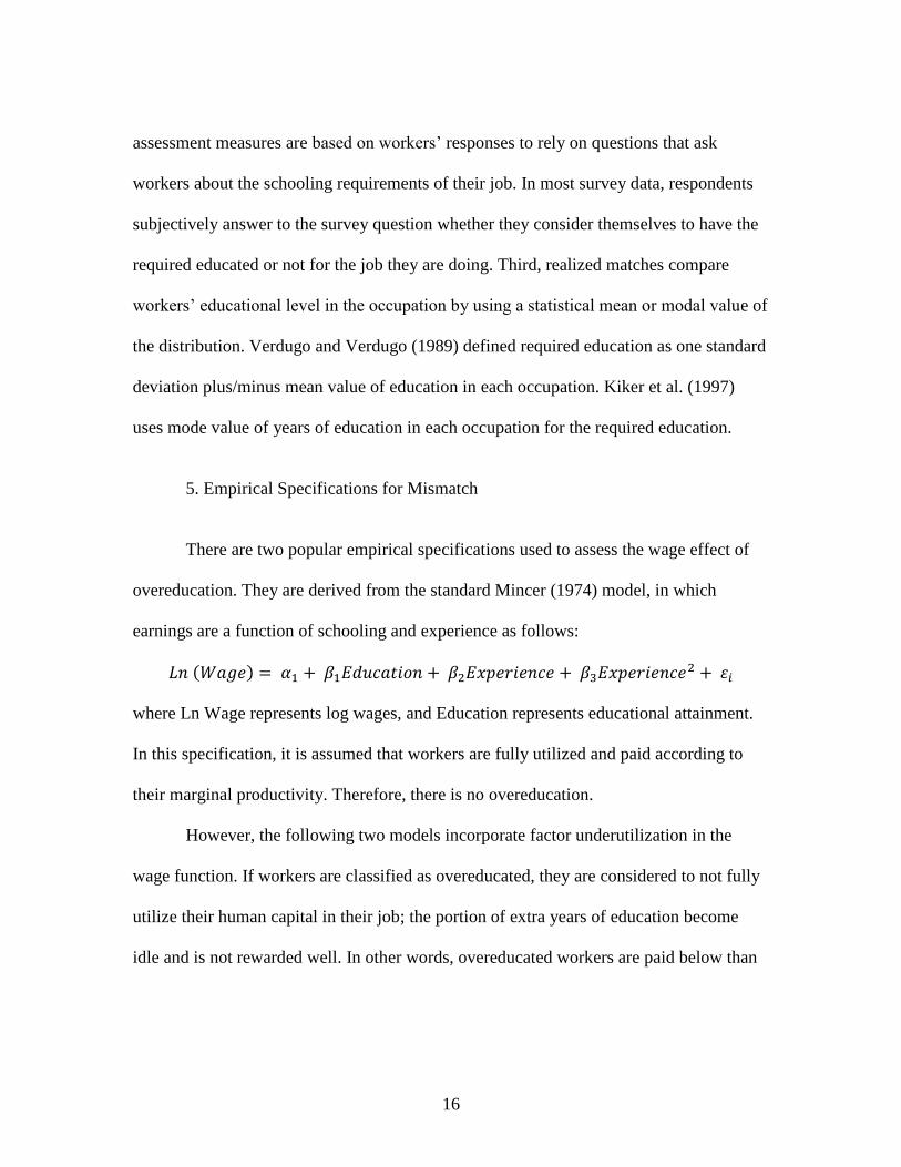
5. Empirical Specifications for Mismatch

There are two popular empirical specifications used to assess the wage effect of

overeducation. They are derived from the standard Mincer (1974) model, in which

earnings are a function of schooling and experience as follows:

𝐿𝑛 (𝑊𝑎𝑔𝑒) = 𝛼1 + 𝛽1𝐸𝑑𝑢𝑐𝑎𝑡𝑖𝑜𝑛 + 𝛽2𝐸𝑥𝑝𝑒𝑟𝑖𝑒𝑛𝑐𝑒 + 𝛽3𝐸𝑥𝑝𝑒𝑟𝑖𝑒𝑛𝑐𝑒2 + 𝜀𝑖

where Ln Wage represents log wages, and Education represents educational attainment.

In this specification, it is assumed that workers are fully utilized and paid according to

their marginal productivity. Therefore, there is no overeducation.

However, the following two models incorporate factor underutilization in the

wage function. If workers are classified as overeducated, they are considered to not fully

utilize their human capital in their job; the portion of extra years of education become

idle and is not rewarded well. In other words, overeducated workers are paid below than

17

their marginal productivity, while workers are paid based on marginal productivity in

neoclassical economics.

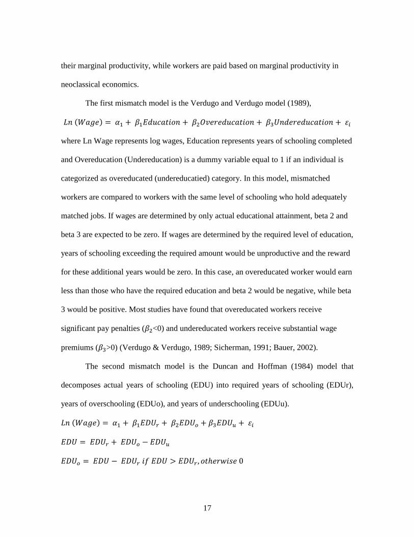
The first mismatch model is the Verdugo and Verdugo model (1989),

𝐿𝑛 (𝑊𝑎𝑔𝑒) = 𝛼1 + 𝛽1𝐸𝑑𝑢𝑐𝑎𝑡𝑖𝑜𝑛 + 𝛽2𝑂𝑣𝑒𝑟𝑒𝑑𝑢𝑐𝑎𝑡𝑖𝑜𝑛 + 𝛽3𝑈𝑛𝑑𝑒𝑟𝑒𝑑𝑢𝑐𝑎𝑡𝑖𝑜𝑛 + 𝜀𝑖

where Ln Wage represents log wages, Education represents years of schooling completed

and Overeducation (Undereducation) is a dummy variable equal to 1 if an individual is

categorized as overeducated (undereducatied) category. In this model, mismatched

workers are compared to workers with the same level of schooling who hold adequately

matched jobs. If wages are determined by only actual educational attainment, beta 2 and

beta 3 are expected to be zero. If wages are determined by the required level of education,

years of schooling exceeding the required amount would be unproductive and the reward

for these additional years would be zero. In this case, an overeducated worker would earn

less than those who have the required education and beta 2 would be negative, while beta

3 would be positive. Most studies have found that overeducated workers receive

significant pay penalties (𝛽2<0) and undereducated workers receive substantial wage

premiums (𝛽3>0) (Verdugo & Verdugo, 1989; Sicherman, 1991; Bauer, 2002).

The second mismatch model is the Duncan and Hoffman (1984) model that

decomposes actual years of schooling (EDU) into required years of schooling (EDUr),

years of overschooling (EDUo), and years of underschooling (EDUu).

𝐿𝑛 (𝑊𝑎𝑔𝑒) = 𝛼1 + 𝛽1𝐸𝐷𝑈𝑟 + 𝛽2𝐸𝐷𝑈𝑜 + 𝛽3𝐸𝐷𝑈𝑢 + 𝜀𝑖

𝐸𝐷𝑈 = 𝐸𝐷𝑈𝑟 + 𝐸𝐷𝑈𝑜 − 𝐸𝐷𝑈𝑢

𝐸𝐷𝑈𝑜 = 𝐸𝐷𝑈 − 𝐸𝐷𝑈𝑟 𝑖𝑓 𝐸𝐷𝑈 > 𝐸𝐷𝑈𝑟 , 𝑜𝑡ℎ𝑒𝑟𝑤𝑖𝑠𝑒 0

18

𝐸𝐷𝑈𝑢 = 𝐸𝐷𝑈𝑟 − 𝐸𝐷𝑈 𝑖𝑓 𝐸𝐷𝑈 < 𝐸𝐷𝑈𝑟 , 𝑜𝑡ℎ𝑒𝑟𝑤𝑖𝑠𝑒 0

In this model, beta 1 is the return to years of required schooling (required education), beta

2 is the return to an additional year of schooling beyond those required (overeducation),

and beta 3 is the return to a year of schooling below the schooling requirement

(undereducation). Most studies have found that the extra years of schooling have a

positive wage effect but smaller than the return to years of required schooling (𝛽1 >

𝛽2>0), while return to years of underschooling is negative (𝛽3<0). Compare to the

Verdugo and Verdugo model, beta 1 and beta 2 must be interpreted relative to workers in

the same occupation who are correctly matched. Human capital theory implies equal

returns 𝛽1 = 𝛽2 = −𝛽3. Job competition theory is a demand-side theory, where marginal

productivity is taken as a fixed characteristic of a particular job and is not related to the

worker. It implies zero returns to years of over and under education, 𝛽2 = 𝛽3 = 0

(Duncan & Hoffman, 1981; Rumberger, 1987; Sicherman, 1991)

6. Job Mismatch and Productivity

Tsang and Levin (1985) questioned the relationship between overeducation and

productivity. Based on industrial psychology literature, they claimed that overeducated

workers are more likely to be dissatisfied with their jobs and exhibit counterproductive

behavior in the workplace.

Tsang (1987) examined the impact of the underutilization of workers’ educational

skills on the production of output of a firm based on the Tsang-Levin model of

19

production. He used the employees of 22 U.S. Bell companies over 1981 to 1983. His

three-step approach showed a negative impact of overeducation on firm productivity.

Ramos et al., (2009) examined impacts of overeducation on the regional

economic growth in 229 European regions in nine countries by using IPUMS

International for 1995, 2000, 2005. They used both cross-sectional and panel regression.

They found that both the percentage of properly educated workers and the percentage of

over-educated workers have positive and statistically significant impacts on per capita

GDP growth. Especially, the magnitude of the coefficient for the percentage of over-

educated workers is greater than the coefficient for the percentage of properly educated

workers. The results reveal that at the regional level as an aggregation, overeducation

might be seen more as an investment than as a cost, although overeducated individuals

obtain a smaller wage than individuals who have required education. In other words, they

insist that the economic impact of overeducation is different between the individual level

and the aggregation level.

7. Quintile Regression

Hartog et al, (2001) examined the evolution of the returns to education in Portugal

over the 1980s and early 1990s. Quintile regression analysis reveals that the effect of

education is not constant across the conditional wage distribution. They are higher for

those at higher quintiles in the conditional wage distribution. Education affects wages

differently at different parts of the distribution. The return to a year of education required

and the return to a year of education above the job requirement increase as one moves

20

upwards in the conditional wage distribution. The penalty for a year of education below

that required for the job also tends to increase at higher quintiles, but at a much slower

pace.

McGuinness and Doyle (2004) examined the impacts of overeducation on income

quantiles for a cohort of Northern Ireland graduates. They used a dummy variable for

overeducation and found that the related wage penalty was heavily concentrated on the

lower income quintiles. Especially, overeducation was more predominant amongst lower

ability male graduates.

8. Unobserved heterogeneity

The majority of studies have assumed that mismatch is exogenous and used cross-

sectional data that cannot account for unobserved heterogeneity. Robst (1995) examined

the relationship between college quality and overeducation by using Panel Study of

Income Dynamics (PSID) data for 1976 and 1985. He found a negative relationship

between college quality and the likelihood of being overeducated, and college quality

influences the ability of overeducated workers to exit the classification. College quality is

measured by ACT scores, SAT scores, the amount of education and general expenditure

per student, and a prestige rating developed by Richard Coleman. Those with higher test

scores face a lower likelihood of being overeducated. For the average ACT score, 44% of

the lowest quartile were overeducated in both periods. Of the workers who were

overeducated in 1976, individuals from higher quality colleges were more likely to leave

the classification by 1985. Workers who attended higher quality colleges are found to

21

have a lower probability of being overeducated. There is a negative relationship between

college quality and the probability of being overeducated and a positive relationship

between college quality and the probability of leaving overeducation status.

Bauer (2002) examined the wage effects of educational mismatch by using a

German Socioeconomic Panel (GSOEP) data set with controlling unobserved

heterogeneity. He found that the estimated differences between adequately and

inadequately educated workers become smaller or disappear totally after controlling for

unobserved heterogeneity. A potential problem of the existing studies, however, lies in

the data sets that they have used, since most employ only cross-sectional data. It is

possible that the estimation results of these studies are biased due to unobserved

heterogeneity of individuals. Controlling for unobserved heterogeneity might be

important if the probability of educational mismatch is correlated with innate ability.

Controlling for unobserved heterogeneity might be important if individuals with lower

innate ability need more education to attain a job for which they are formally

overeducated.

Bauer compared results from three different specifications: V-V model, pooled

OLS, Random effects, and Fixed effects. He used two measurements for mismatch: mean

plus/minus one standard deviation and modal value. The results for the pooled OLS

suggest that overeducated male workers earn 10.6% less and undereducated male workers

8% more than male workers with the same amount of education who are working in

occupations which fully utilize their educational level. For both the random effects and

the fixed effects model, the estimated coefficients of the educational mismatch dummies

22

change in the expected direction. In most cases, the absolute values of the estimated

coefficients on the dummies indicating educational mismatch are significantly lower

when unobserved characteristics are accounted for. The estimated effects change

dramatically when one controls for unobserved heterogeneity using panel estimation

techniques. The earnings differences between inadequately educated workers and equally

educated workers who work in occupations for which they are adequately educated

becomes at least smaller, and in most cases disappears totally.

23

CHAPTER THREE

HYPOTHETICAL FRAMEWORK

Figure 3. Hypothetical Framework

< Exogenous Event >

Soviet Launch of

Sputnik

< Policy Outputs >

1. Expanding role of the NSF

2. National Defense Education

Act (NDEA) of 1958

< Policy Effect >

Increase in College

Enrollments

< Labor Market >

Increase in Supply

of Skilled Labor

<Exogenous Changes in Market>

Skill-Biased Technological Change.

International Trade.

< Labor Market >

Increase in Demand

for Skilled Labor

< Policy Process>

Problems Stream

Policy Stream

Politics Stream

< Economic Issues >

1. Occupational Segregation

between skilled and

unskilled workers.

2. Job Mismatch.

3. College Wage Premium.

< Arms Race >

U.S.S.R. vs.

U.S.

< Policy Event >

Educational

Reform in U.S.

<Domestic Program>

Civil Rights

Great Society

< Policy Output>

3. Higher Education Act

(HEA) of 1965

24

Figure 3 shows the hypothetical framework for this paper; the arrows imply

possible causality flow. I claim that there is a cause and effect relationship between

Sputnik and educational reform in U.S. in early 1960s. By introducing a Sputnik into the

educational reform in U.S., I argue that educational reform in U.S. did not arise based on

domestic needs but it was triggered by an exogenous event. First, I use the Arms Race

Model to support the linkage between Sputnik and educational reform in U.S. Second, I

use John Kingdon’s Multiple Streams Model to explain the policy process of producing

policy outputs related with science and defense. Third, the initial purpose of federal

funding was diffused to producing more general human capitals for economic growth

under the subsequent domestic programs such as Civil Rights and Great Society. Fourth,

I focus on three policy outputs related with higher education: NSF, NDEA (1958), and

HEA (1965). Fifth, I interpret the increase in the supply of college graduates as a policy

outcome, combining the NSF, NDEA, and HEA. Sixth, there are three economic issues

that I analyze with an empirical study: occupational segregation between skilled and

unskilled workers, overeducation, and college wage premium.

1. Arms Race Model

Arms Race Model provides theoretical perspectives about the reaction of the

American government reflecting the rivalry relationship between the U.S. and the Soviet

Union during the Cold War. In other words, the American government perceived Sputnik

as more a military threat than a simple scientific and technological achievement. They

thought that if a country is able to govern space, it will be able to dominate over the

world. Therefore, I interpret the reaction of the American government as an extension of

25

the arms race, instead of merely a science educational competition. The following three

arms race models provide a single dominant strategy for American government against

the Soviet launching of Sputnik.

1-1. Richardson’s arms race model

According to the Richardson’s (1960) arms race model between two countries, the

rate of change in a country’s level of armaments is negative to its own level of

armaments, but positive to its enemy’s level of armaments. It is mathematically expressed

by a set of linear differential equations. For example, let’s say the two countries are U.S.

and the Soviet Union. The equations would be as follows:

𝑑(𝐴𝑚𝑒𝑟𝑖𝑐𝑎)

𝑑𝑡= 𝑎 − 𝑏(𝐴𝑚𝑒𝑟𝑖𝑐𝑎) + 𝑐(𝑆𝑜𝑣𝑖𝑒𝑡𝑠)

𝑑(𝑆𝑜𝑣𝑖𝑒𝑡𝑠)

𝑑𝑡= 𝑑 − 𝑒(𝑆𝑜𝑣𝑖𝑒𝑡𝑠) + 𝑓(𝐴𝑚𝑒𝑟𝑖𝑐𝑎)

The coefficients 𝑎 and 𝑑 are “grievances” which derive nations to arm at a constant rate,

and coefficients 𝑏 and 𝑒 are “fatigue and expense” caused by economic burden, and 𝑐 and

𝑓 are called “defense coefficients” which measure each nation’s reaction to its

opponent’s armaments. Thus, the equations tell us that change in America’s armaments

positively relates with the level of Soviet’s armaments and vice versa.

26

Figure 4. Military Expenditure Reaction Functions

It does not mean that there is no equilibrium. Figure 4 shows the military expenditure

response functions for the Soviet Union and America. In the above equations, A

represents America and S represents the Soviet Union. Let’s say that the initial

equilibrium is E1. Considering the arms race, if the Soviet Union increases its military

expenditure, the new equilibrium will be E2, which triggers America’s response, and the

correspondingly increase in military expenditure by America raises the new equilibrium

level of expenditure to E3. Therefore, America’s best reaction is increased military

expenditure corresponding to the Soviets’. However, why does either of the countries try

to break the equilibrium? The following Prisoner’s Dilemma Game gives an answer.

1-2. The Arms Race as a Prisoner’s Dilemma Game

Brams et al. (1979) modeled a Prisoner’s Dilemma Game for the arms race by

with which they explained why one side broke the equilibrium.

E1

E2

E3

Soviet Union

Union

America

27

Table 2. The Arms Race as a Prisoner’s Dilemma Game

USSR

Disarm Arm

US

Disarm

USSR: 0 USSR: 45

US: 0 US: -30

Arm

USSR: -30 USSR: -5

US: 45 US: -5

Table 2 shows a Prisoner’s Dilemma Game for an arms race between two countries,

America and Soviet Union. The numbers in each box are payoffs for the strategy for each

country. According to the payoff, the dilemma in this game is that Arm is the dominant

strategy for both countries. In other words, regardless of the other country’s strategy,

each country obtains a higher payoff by choosing Arm, which means that America’s best

strategy does not depend on whatever the Soviet Union chooses. If both countries choose

Disarm, then payoff is (US: 0, USSR: 0), but there cannot be an equilibrium because each

country has an incentive to choose Arm and thus obtain its highest payoff (US: 45 or

USSR: 45) and imposes the worst payoff on the other player (USSR: -30 or US: -30).

Therefore, choosing Arm, (US: -5, USSR: -5), is the unique equilibrium.

1-3. Competitive Arms Accumulation Model

Ploeg and Zeeuw (1990) show a competitive arms accumulation model

between two countries in the form of utilities, which depend on consumption, leisure and

28

the characteristic defense. In their model, government finances the investment in arms by

non-distortionary taxation and representative household maximizes utility and firm

maximizes profits.

Government’s budget constraint: ɡ = τ

ɡ: government investment, τ: lump-sum taxes

Household maximizes utility: 𝑢(𝑐, 𝑙, 𝑑) subject to budget constraint 𝑜 ≤ 𝑐 ≤ 𝑤𝑙 + 𝜋 − 𝜏

𝑐: 𝑐𝑜𝑛𝑠𝑢𝑚𝑝𝑡𝑖𝑜𝑛, 𝑙: 𝑙𝑎𝑏𝑜𝑟 𝑠𝑢𝑝𝑝𝑙𝑦, d: defense, w: real wage, π: profits, τ: lump-sum

taxes.

Firm maximizes profit: 𝜋 = 𝑓(𝑙) − 𝑤𝑙

𝑓: 𝑎 𝑐𝑜𝑛𝑐𝑎𝑣𝑒 𝑝𝑟𝑜𝑑𝑢𝑐𝑡𝑖𝑜𝑛 𝑓𝑢𝑛𝑐𝑡𝑖𝑜𝑛, 𝑤 = 𝑓 ,(𝑙)

Goods market equilibrium: 𝑓(𝑙) = 𝑐 + 𝑔

In the model, utility is assumed to be separable in defense, which is a function of a

country’s own weapon stock and foreign weapon stock, that is d=D (a, a*), where ‘a’

denotes own weapon stock and ‘a*’ denotes foreign weapon stock. It is assumed that

defense is an increasing function of one’s own weapon stock, a, 𝑑𝐷 𝑑𝑎⁄ > 0, while it is a

decreasing function of the foreign weapon stock, a*, 𝑑𝐷 𝑑𝑎∗⁄ < 0. Moreover, equal

increase in the weapon stocks of two countries leaves the level of defense unaffected,

which is 𝑑𝐷 𝑑𝑎⁄ = − 𝑑𝐷 𝑑𝑎∗⁄ > 0. If we assume that the two countries are America and

the Soviet Union, ‘a’ represents the level of armaments of U.S. and ‘a*’ represents the

level of armaments of the Soviet Union. Therefore, for the representative household in

the U.S., utility from defense is increased by the level of armaments of the U.S. but

decreased by increasing the level of armaments of the Soviet Union. To satisfy

29

equilibrium condition, 𝑑𝐷 𝑑𝑎⁄ = − 𝑑𝐷 𝑑𝑎∗⁄ , the American government should increase

the level of armaments, as well as tax collections.

In summary, Richardson’s linear differential equations for the arms race model

are inversely related to a country’s own weapon stocks because of economic burden, but

positively related to the competing country’s weapon stock because of the threat. Brams’

Prisoner’s Dilemma Game for the arms race shows that a country can obtain the highest

payoff by arming, regardless of the competitive country’s strategy. Ploeg and Zeeuw’s

competitive arms accumulation model tells us that increase in the weapon stocks of the

competitive country causes disutility of the representative household in the home country.

Equilibrium is achieved when the level of weapon stocks are equal in both countries.

Therefore, the responses of the American government, which are educational reform and

expanding government expenditure for armaments, are justified by these three arms race

models.

2. Agenda Setting by Kingdon’s Multiple Streams Model

Kingdon’s multiple streams model is a popular theoretical perspective used to

explain the dynamic and complex agenda-setting process. Kingdon’s Multiple Streams

Policy Making is based on three independent process streams: problems, policies, and

politics. When any two streams are coupled, they change a circumstance and enhance the

probability of an issue being on the government’s decision agenda (Young et al. 2010).

Sometimes the policy window is opened by a problem that presses in on government, or

at least comes to be regarded as pressing (Kingdon, 2013). According to Kingdon, the

30

problem stream explains why some problems come to occupy the attention of

government officials. The problem stream involves the process of problem recognition by

indicators, focusing events, and feedback. Indicators are used to assess the magnitude of

the condition, a focusing event draws attention to some conditions more than to others,

and officials learn about conditions through feedback about the operation of existing

programs. Conditions come to be defined as problems, and have a better chance of rising

on the agenda, when we come to believe that we should do something to change them.

The political streams model explains the relative prominence of issues on official

agenda. Independently of problem recognition, political events flow along according to

their own dynamics and their own rules. Participants perceive a swing in national mood,

elections bring new administrations to power and new partisan or ideological

distributions to Congress, and interest groups of various descriptions press their demands

on government. Policy stream addresses alternative specifications by members of the

policy community. Policy communities include policy actors inside and outside of the

government. I want to explain the educational agenda setting in the U.S. inspired by

Soviet launching of Sputnik by applying Multiple Streams Model.

2-1. Problem Stream

Problem stream focuses on the exogenous events of the sequential success of

launching Sputnik 1, Sputnik 2, and Sputnik 3, and its impact on American society and

corresponding problem recognition by Americans. Soviet Union launched world’s first

man-made artificial Earth satellite, Sputnik 1, on October 4, 1957. The American public,

31

politicians, and military associates were surprised because the launching of a satellite was

a technological, scientific, and military achievement. Moreover, the success of Sputnik 1

seemed to have changed minds around the world regarding a shift in technological

leadership and military power to the Soviet Union from the United States.

When Americans witnessed the great success of Soviet space technology with the

launching of Sputnik in 1957, they stood in fear of the new aspect of the Soviet threat

(Lucena 2005, p.27). Some sectors of industry and the public responded by incorporating

the new objects of fear into consumer goods. Restaurants began serving

“Sputnikburgers,” and bars sold “Sputnik cocktails” (Lucena 2005, p.27). When

Americans get worried, their fear quickly spreads to the stock market. On October 7, the

Dow Jones index declined 6.32 points and two weeks later the market experienced its

largest one-day loss in two years (Degroot 2006, p.63). A month after the launch, opinion

polls showed that a majority of Americans considered Sputnik a blow to their nation’s

prestige, and a roughly equal percentage believed that the United States was behind the

Soviets in space research, with a significant number believing the gap “dangerously”

large (Degroot 2006, p. 67-68).

In a field-by-field survey of all Russian sciences, scientific experts from all over

the world agreed that, although the USSR lagged in some fields of applied science, it led

the U.S. in most fields of basic scientific research. “What is important about the Russian

satellites is the base of science beneath them,” (Lucena 2005, p.29). Scientific academics

(Vannevar Bush, James Conant, and James Killian) defined the new problem facing the

32

American nation not only in terms of basic science and scientists but also in terms of

science education (Lucena 2005, p.30).

A group of scientists, James Conant (Chairman of the National Science Board),

Nicholas DeWitt (the NSF commission), and Alan Waterman (Director of NSF) criticized

the U.S. for producing too many businessman, lawyers, and humanities scholars and not

enough scientists and engineers (Lucena 2005, p.22). A couple of months after Sputnik,

Eisenhower made an official statement that national security is for the most critical

problem of all for the American people and asserted that the United States needed

thousands more scientists than were currently active (Lucena 2005, p.30). After Sputnik

went up, all the talk was about the “fact” that Russian kids went to school for six hours a

day, six days a week, and got shorter summer holidays than American children (Degroot

2006, p.76). An official report by the Department of Health, Education and Welfare made

the preposterous claim that all Russian children took five years of physics, four of

chemistry, and five of mathematics (Degroot 2006, p.76).

On November 3, 1957, the Soviet Union launched Sputnik 2, a satellite weighing

about 500 kilos, about the size of small car. Even more remarkable than the weight was

the fact that the capsule contained a dog named Laika, and the systems necessary to keep

it alive for a short time (Degroot 2006, p.80). Once Laika went into orbit, Soviet and

American perceptions of space changed radically. Up until that point, the important issue

was the Soviet ability to lift very heavy objects into orbit. That capability seemed to

threaten U.S. security (Degroot 2006, p.81).

33

On December 6, 1957, the United States made its first attempt to place a satellite

in orbit. The Vanguard team had a relatively new rocket that had not been fully tested

(Degroot 2006, p.82). At 11:44:55 AM on Friday, December 6, 1957, the slender rocket

rose slowly from its launch pad. After two seconds, and at an elevation of about four feet,

it abandoned the struggle. It shuddered, then collapsed in a fiery heap. The American

satellite was nicknamed Stayputnik, Flopnik, Oopsnik, Pfftnik, and Sputternik (Degroot

2006, p.83). Sputnik 2 continued to broadcast its signal until early December, thus

pouring salt on American wounds (Degroot 2006, p.84). The president was identified

with Vanguard’s failure and therefore had to share its ignominy (Degroot 2006, p.87).

Eisenhower’s space woes were compounded by talk of a missile gap. On

November 12, 1957, in the wake of Sputnik, a national intelligence estimate forecast that

the Soviets would have five hundred operational ICBMs by the end of 1962, while the

United States would have only around sixty-five. On the strength of this evidence,

Eisenhower was lambasted for endangering the security of the United States, even though

the American lead in bombers and total nuclear weapons was still huge (Degroot 2006,

p.91).

For most Americans, the “missile gap” and the space race were two sides of the

same coin. The public was growing increasingly impatient with Eisenhower’s

leadership—or lack thereof. They demanded action, especially after the success of

Explorer 1 was followed quickly by the embarrassing failure of a second Vanguard, and

then by the crash of Explorer 2 (Degroot 2006, 92).

34

On May 15, 1958, the Soviets again emphasized their supremacy in heavy lifting

by launching Sputnik 3, a behemoth weighing nearly 1,400 kilos. The new capsule, one

Russian scientist stressed, “could easily carry a man with a stock of food and

supplementary equipment.” (Degroot 2006, 94).

In the problem stream, Americans started to recognize that they needed to address

three specific deficits: (1) the numbers of scientists, (2) science education and curriculum,

and (3) a lack of science education from K-12 to college, as well as further basic

scientific researches in higher education. Prior to 1957, the problem was defined as a

matter of numbers in the armed forces (Lucena 2005, p.31). With a more accurate

recognition of the problems facing the United States and its space program, scientists, the

White House, and Congress started to find policies to solve these specific problems.

2-2. Policy Stream

The American government recognized that the Soviet Union was far ahead of

America in basic scientific research. Immediately after Sputnik, one of the first requests

by both Congress and the President was to find out the number of scientists and engineers

available to meet the needs of the nation (Lucena 2005, p.46).

The popular media had better success in shifting the national attention from the

shortfall in numbers to science education (Lucena 2005, p.30). In early 1958, Life

magazine ran a five-part series on the “Crisis in Education” that explored every aspect of

“the field of battle for future brain power-the U.S. and the Russian schools.” (Lucena

2005, p.30). The series of articles concluded with James Conant’s blueprint for high

35

school curriculum in which he pointed out the basic problem of U.S. education, and

proposed a meritocratic educational system (Lucena 2005, p.31).

President Eisenhower selected MIT President James Killian as his full-time

Special Assistant for Science and Technology and established the President’s Science

Advisory Committee (PSAC) (Lucena, 38). In 1951, President Harry S. Truman had

established the Science Advisory Committee as part of the Office of Defense

Mobilization (ODM). As a direct response to the launches of the Sputnik 1 and Sputnik 2,

on October 4 and November 3, 1957, the Science Advisory Committee was upgraded by

President Eisenhower to the President's Science Advisory Committee (PSAC) and moved

to the White House on 21 November 1957. These appointments opened the White House

doors to scientific academism. Robert Kreidler claims that with these appointments

“members of the scientific community were given direct access to the President and an

established means of expressing themselves on matters of science policy (Lucena, 38).

On Oct 10, 1957, only six days after Sputnik’s launch, director of the National

Science Foundation (NSF) Alan Waterman, beginning his quest for money for science

education, told the National Security Council the necessity for effective steps toward

maintaining progress in basic science and the training of capable scientists and engineers

(Lucena, p.41). The President’s budget and subsequent congressional appropriation for

FY 1959 resulted in an increase of 300 percent, to approximately $61 million, for existing

NSF educational programs and for the initiation of new ones. The percentage of the

NSF’s total budget ($137 million) devoted to education reached an all-time high of 45%

36

(Lucena, p.41). NSF began to emerge as an institutional solution for the manpower

political problem of the 1960s (Lucena 2005, p.38).

When asked by legislators to explain what was wrong with American science,

German rocket scientist Werner Von Braun called for a massive injection of money and

effort to be directed to the teaching of science (Degroot 2006, p.75). Legislators

responded with calls for a Manhattan Project for space and a West Point for science

(Degroot 2006, p.75). The Advanced Research Projects Agency was created to make sure

that Americans were kept busy with technological projects, not exclusively related to

space, designed to make sure that the United States would never again fall victim to an

embarrassment like Sputnik (Degroot 2006, p.75). The National Defense Education Act

(NDEA) was rocketed through Congress and signed into law by Eisenhower on

September 2, 1958 (Degroot 2006, p.75). A four-year plan for boosting American

education, it provided millions for the purchase of scientific equipment for schools, in

addition to loans and grants for those inclined to go into teaching (Degroot 2006, p.75).

Before long, the NDEA was giving out scholarships to almost any high school graduate

who could present a credible case for wanting to study science at a university (Degroot

2006, p.75).

Immediate policies and proposals emerged after Sputnik that involved the

extension of NSF’s role to nurture elite scientists, establishing the President’s Science

Advisory Committee (PSAC), and the National Defense Education Act (NDEA) of 1958.

The purposes of proposed policies were not an increase in armed forces but in enhancing

science education and producing scientists needed for national security.

37

2-3. Politics Stream

The politics stream focuses on the interactions between political actors, Congress,

White House, and interest groups with regard to changes in national mood and elections

that bring new administrations to power. Sputnik brought a test on Presidential leadership

and Congressional ability to overcome an imbalance of the superpowers and provide an

improved course for the United States’ science program.

Initially, President Eisenhower was not surprised by Sputnik because he had

expected the event because of information derived from U2 spy planes’ flyover photos.

President Eisenhower steadfastly refused to panic (Degroot 2006, p.77). On October 9,

Eisenhower told a press conference that he saw “nothing…that is significant in that

development as far as security is concerned, except…it does definitely prove the

possession of the Russian scientists of a very powerful thrust in their rocketry…The mere

fact that this thing orbits involves no new discovery of science…so in itself it imposes no

additional threat to the United States.” (Degroot 2006, p.77). He went on to allege that

the reason the Russians had been first in space was because they had “captured all the

German scientists” in Peenemunde (Degroot 2006, p.77). He played five rounds of golf

during the week after the launch, perhaps to drive home the suggestion of calm (Degroot

2006, p.66). Meanwhile, James Hagerty, the White House press secretary, told

journalists that the satellite, while of great scientific interest” did not come as any

surprise; we have never thought of our program as in a race with the Soviet.” (Degroot

2006, p.66).

38

Sensing an electoral opportunity, Senator Lyndon Johnson seized the chance to

weight in: “The issue is one which, if properly handled, would blast the Republicans out

of water, unify the Democrat Party, and elect you President.” an aid told the ambitious

senator (Degroot 2006, p.69). Before Sputnik, the Democrats were mired in gloom. The

segregation issue, which had split the party, seemed likely to destroy their chances of

regaining the White House (Degroot 2006, p.69). “The Roman Empire,” Johnson

claimed, “controlled the world because it could build roads. Later the British Empire was

dominant because it had ships. In the air age we were powerful because we had airplanes.

Now the communists have established a foothold in outer space.” (Degroot, p.70). The

history lesson might have been crude and simplistic, but the American people lapped it

up. On another occasion, he claimed: “From space the masters of infinity would have the

power to control the Earth’s weather, to cause drought and flood, to change the tides and

raise the levels of the sea, to divert the Gulf Stream and change temperate climates to

frigid.” (Degroot 2006, p.70). He promised that, whatever the administration’s space

budget, he would convince Congress to increase it, a promise that alarmed the fiscally

conservative Eisenhower. (Degroot 2006, p.70).

In the November edition of Missiles and Rockets, Editor Erik Bergaust wrote “An

Open Letter to President Dwight D. Eisenhower.” The editorial expressed all the

emotions the president feared. “This is the age of science,” Bergaust warned Eisenhower.

“This is the era of intellectual, uninhibited thinking. Tomorrow is here. And you, as the

leader of the greatest nation on Earth, must see to it that this nation will be out in front as

mankind advances into the space age.” (Degroot 2006, p.81). Bergaust called for a

39

cabinet-level science adviser, a coherent space program, a new space agency, and

missions to the Moon, Venus, and Mars (Degroot 2006, p.81).

Eisenhower realized that he could not simply ignore the American people’s

feelings of inadequacy. On November 7, before a radio and television audience, he

delivered the first of his “Science in National Security” talks from the White House. It

was in part shaped by a report from the Office of Defense Mobilization and Science

Advisory Committee (ODM-SAC) on the need to improve public appreciation of science,

strengthen the partnership between sciences and the federal government, increase support

for basic research, especially in the Department of Defense, and reform science education

(Wang 2008, p.81). In this address, Eisenhower highlighted science not only as the

driving force in the defense of America, but also as a key to the nation’s future security

and prosperity (Wang 2008, p.82). In response to critics who derided the state of

scientific education in the United States, the president announced that he was appointing

James Killian of MIT the first White House science adviser. (Degroot 2006, p.81). A

week later, in another speech on national security, Eisenhower expanded on the

importance of science education and basic research: “My scientific advisers place this

problem (science education) above all other immediate tasks of producing missiles, of

developing new techniques in the Armed Services.” (Wang 2008, p.82). The upgrade of

the Office of Defense Mobilization and Science Advisory Committee (ODM-SAC) into

the President’s Science Advisory Committee (PSAC) in the White House proceeded soon

after the Killian appointment (Wang 2008, p.82).

40

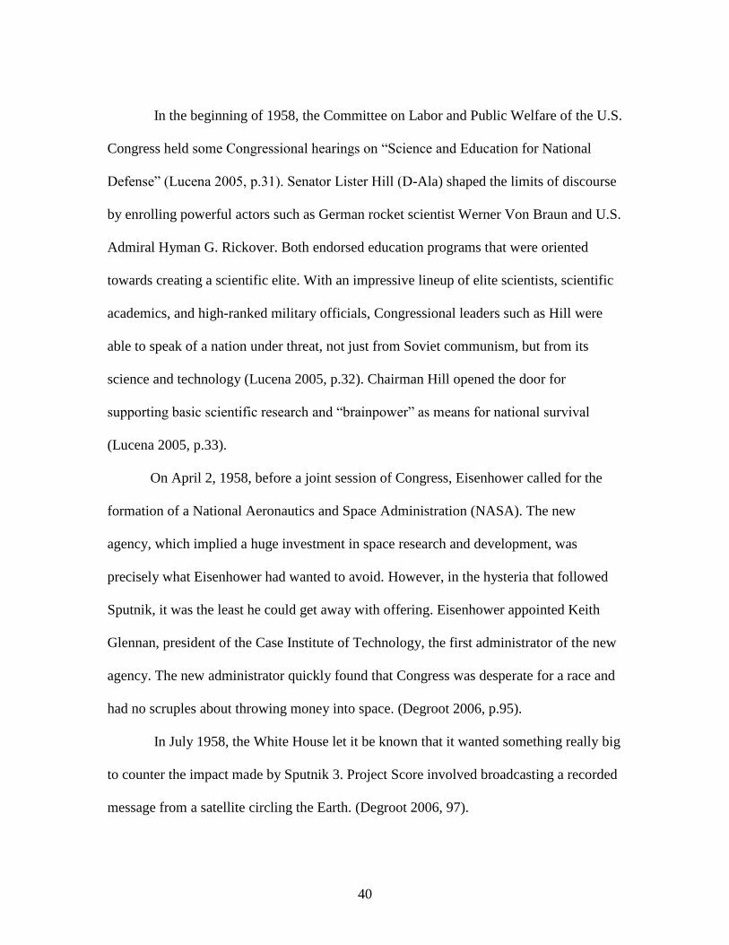
In the beginning of 1958, the Committee on Labor and Public Welfare of the U.S.

Congress held some Congressional hearings on “Science and Education for National

Defense” (Lucena 2005, p.31). Senator Lister Hill (D-Ala) shaped the limits of discourse

by enrolling powerful actors such as German rocket scientist Werner Von Braun and U.S.

Admiral Hyman G. Rickover. Both endorsed education programs that were oriented

towards creating a scientific elite. With an impressive lineup of elite scientists, scientific

academics, and high-ranked military officials, Congressional leaders such as Hill were

able to speak of a nation under threat, not just from Soviet communism, but from its

science and technology (Lucena 2005, p.32). Chairman Hill opened the door for

supporting basic scientific research and “brainpower” as means for national survival

(Lucena 2005, p.33).

On April 2, 1958, before a joint session of Congress, Eisenhower called for the

formation of a National Aeronautics and Space Administration (NASA). The new

agency, which implied a huge investment in space research and development, was

precisely what Eisenhower had wanted to avoid. However, in the hysteria that followed

Sputnik, it was the least he could get away with offering. Eisenhower appointed Keith

Glennan, president of the Case Institute of Technology, the first administrator of the new

agency. The new administrator quickly found that Congress was desperate for a race and

had no scruples about throwing money into space. (Degroot 2006, p.95).

In July 1958, the White House let it be known that it wanted something really big

to counter the impact made by Sputnik 3. Project Score involved broadcasting a recorded

message from a satellite circling the Earth. (Degroot 2006, 97).

41

Initially, President Eisenhower tried to avoid a race to space with the Soviet

Union because of the economic burden, but the media formed public opinion on demand

for science education, and the continuous success of Sputnik 2 and Sputnik 3 made him

take actions. He organized a new science committee and appointed new leadership, and

Congress approved a budget for government agencies and passed an educational act to

improve quality and quantity in science education and scientists. Overall, problem

stream, policy stream, and politics stream all played a part in improving and developing

scientific manpower in America.

42

CHAPTER FOUR

EQUALITY OF OPPORTUNITY

In this chapter, I want to contemplate government financial aid for education in

viewpoints of paternalism and public choice because the nature of policy issues on

education is its redistributive aspect and increasing human capitals. In addition, President

Kennedy and President Johnson were interested in civil rights, eliminating poverty, and

racial injustice. Therefore, science and defense-focused educational reform was shifted to

produce more general human capital for economic growth of the nation and to the

increase of opportunity to access higher education by poor students. Johnson passed the

Higher Education Act on November 8, 1965 by his Great Society domestic agenda. HEA

1965 was designed to provide financial aid to the needy students from lower income

families. Redistributive policies that transfer value to the less advantaged at the expense

of the more advantaged require the convergence of significant forces (Hannah 1996,

p.502). For example, the initiation of basic educational opportunity grants for

postsecondary students with exceptional financial need in HEA 1965 required

presidential leadership, Congressional support, a broad national constituency in the ‘war

on poverty’, the momentum of the civil movement, and a growing economy that could

afford redistribution (Hannah 1996, p.502).

1. Paternalism

Eyal Zamir (2007) defines paternalism as intervention in a person’s freedom

aimed at furthering his or her own good. Gerald Dworkin (1972), however, suggests that

43

paternalism is justified only to preserve a wider range of freedom for the individual in

question. He says that the interference with a person’s liberty of action justified by

reasons referring exclusively to the welfare, good, happiness, needs, interests, or values

of the person being coerced. He provides examples of paternalistic interference: laws

requiring motorcyclists to wear safety helmets when operating their machines, laws

forbidding persons from swimming at a public beach when lifeguards are not on duty,

and so on, which place restrictions on the liberty of individuals. I interpret Dworkin’s

paternalistic intervention as an intent to reduce disutility from what otherwise would have

happened with no intervention.

Isbister (2004) asserts that social justice has three components: equality, freedom,

and efficiency. He classifies equality as equality of opportunity and equality of resources,

and distinguishes “freedoms-to” and “freedoms-from”. According to him, “freedoms-to”

are freedoms to do various things such as freedom to worship, speak, publish, assemble,

and petition the government for redress of grievances. “Freedoms-from” are freedoms

from such afflictions as hunger, poverty, illiteracy, sickness, and homelessness (Isbister

2004, p.16). I think that publicly provided education has a duality if one’s utility of being

educated is at least of the same magnitude with one’s disutility of being illiterate.

Thaler and Sunstein (2003) suggest the idea of libertarian paternalism. Traditional

paternalism involves coercion, although the intervention has a good motive. Thaler and

Sunstein define libertarian paternalism as the intervention that nudges people in the

direction that will promote their welfare with no coercion of choice. The government

provides financial aid for higher education with no coercion of going to college, but

44

influences the decision of college enrollment by reducing the price of college education.

As long as there is no penalty for dropping out of college due to lack of financial aid, the

financial aid for college education is not coercion. Financial aid may bring a substitution

effect by reducing the opportunity costs of staying in school, but also bring an income

effect by reducing the price of education. Subsidies can reduce costs and thereby magnify

the relative benefits.

Johnson (1984) provides three ways to justify government subsidization of higher

education. First, there are gross social benefits from highly educated population. Second,

it is socially inefficient not to provide the optimum amount of training to bright young

people just because their families happen to be poor. Third, taxation affects private

human capital accumulation decisions. Too high an income tax may undervalue of

present discounted future income relative to costs after graduating college, which may

affect the decision of college enrollments. Therefore, subsidy can be used to correct for

the distortions caused by the tax system.

According to Isbister (2004), efficiency means getting the best out of the available

resources. Therefore, it is socially inefficient for bright young people from poor

households to be left with inadequate education because society does not get the best out

of the available resources and also does not provide them a “freedom-to” receive

education or a “freedom-from” being illiterate. A paternalistic state must provide the

population access to receive public education and also prevent the population from being

illiterate, and thus population can have a wider range of freedom.

45

Leonard et al (2000), however, assert that truly paternalistic policies are

distinguishable from interventions intended to correct market failures that arise from

insufficient information, because even a non-paternalistic state can provide information

to the market. They insist that a paternalist is logically required to believe that the

intervener is better placed than the paternalized person to judge the latter’s welfare.

In terms of educational costs, parents are expected to contribute to the cost of

their children’s postsecondary education. However when their ability is limited,

government can provide an educational subsidy based on need. Trostel (2002) insists that

a subsidy in the form of public provision has the potential to be the most efficient

educational policy because it stimulates investment in human capital. He argues that there

is no practical policy to lower the price of the primary input in human capital production.

In other words, it is impractical to lower the opportunity cost of staying in school.

Therefore, it is not practically possible to stimulate investment in education if there is no

public provision of a subsidy.

2. Public Choice

Public Choice sees voters, politicians, and bureaucrats as self-interested agents

who maximize their own utility. Mancur Olson (1993) shows how self-interested utility

maximization motivates leaders in both autocracy and democracy to provide public goods

to their domains. Thus altruism neither of a necessary condition nor a sufficient condition

for providing public goods, especially for an autocrat.

46

Mancur Olson (1993) introduces a new theory of how autocracies and

democracies emerge from anarchy and affect economic development. Of particular

interest is his theory about how a rational self-interested autocrat is motivated to provide

public goods to his citizens, because it is the usual expectation that dictators are more

likely to exploit the population ruthlessly in their domains rather than spending for public

goods. In his theory, however, he emphasizes peaceful order and providing public goods

to make society productive as common factors for both types of government, dictatorship

and democracy. Under anarchy, victims of violence and theft lose what they produced

and also lose the incentive to produce any more goods because roving bandits do not

have any encompassing interest in society. When a roving bandit may steal goods

occasionally and depart immediately, inhabitants can have little incentive to produce or

way to secure accumulate goods. However, if a bandit settles down as a stationary bandit,

he may have an encompassing interest in his domain that encourages him to support a

peaceful order and public goods that increase productivity. According to Olson, having a

dictator as a stationary bandit is better for both the population and the bandit himself in

the sense that the bandit can monopolize theft in the form of taxes regularly and

continuously, and inhabitants can have their own “safe” income after tax and are

provided protection from other thieves. Such protections from other thieves and property

rights on after-tax goods increase output in the society and thus provide more tax

payments to the leader (the stationary bandit). Contrary to the roving bandits, under the

stationary bandit, inhabitants are not a resource to be exploited but a source of tax

payments. Therefore, the leader as stationary bandit has an incentive to protect

47

inhabitants in his domain from domestic violence and foreign thieves, and to provide any

public goods that can increase taxable income up to the point where the marginal cost of

providing public goods is equal to the marginal income from increased output.

The rational self-interested autocrat chooses the revenue-maximizing tax rate

instead of behaving like the wolf that preys on the elk. Therefore, monopolization of theft

and the protection of the tax-generating population replaces anarchy with government.

The rational stationary bandit takes only a part of income in taxes, while he has an

incentive to provide other public goods, which can increase taxable income. By providing

more public goods he can thieve more from his subjects in the form of taxes than he

could have stolen by being a roving bandit. Olson says that this mutual incentive from

settling a government is very effective, even in the democratic community, because a

self-interested incumbent president will maximize his chances of reelection by making

the voters better off.

3. Expansion of Reform

John F. Kennedy became the 35the President of the United States in 1961. He

served as President from January 1961 until his assassination in November 1963.

Kennedy’s time in office is also marked by high tensions with Communist states, Soviet

Union and Cuba in particular. Since when he was a senator, he was interested in civil

rights movements. Kennedy cast a procedural vote on the President Eisenhower’s bill for

the Civil Rights Act of 1957. His concerns about civil rights were reflected in his

domestic policy, which was called the New Frontier. Through the New Frontier, he

ambitiously promised federal funding for education, medical care for the elderly,

48

economic aid to rural regions, and government intervention to halt the recession.

Moreover, he promised to eliminate racial discrimination. Especially, his racial

integration was very well reflected in his Executive Order 10925, which required

government contractors to take affirmative action to ensure that employees are treated

fairly without regard to their race, creed, color, or national origin.

On December 14, 1961, Kennedy signed the executive order creating the

Presidential commission on the Status of Women concerning on sexual discrimination.

On June 10, 1963, Kennedy signed the Equal Pay Act of 1963 aiming at abolishing wage

disparity based on sex. On June 11, 1963, Kennedy gave his famous civil rights address,

on national television and radio to provide equal access to public schools and voting

rights.

Sputnik-inspired educational reform was concentrated in science and national

defense related educations led by NSF and NDEA, during the administration of President

Eisenhower. However, as described above, until assassinated on November 22, 1963,

Kennedy had many concerns on civil rights, racial integration, and equal opportunity of

education. These concerns of Kennedy’s domestic policy started to shift the emphasis of

educational reform from science to equal opportunity to access all level of educations

with no racial or sexual discrimination. It does not mean that Kennedy gave up science

education or the space race with the Soviet Union. In fact, he became eager for the United

States to take the lead in the space race by a manned Moon landing (the Apollo program).

On July 20, 1969, almost six years after Kennedy's death, Apollo 11 landed the first

manned spacecraft on the Moon.

49

President Lyndon Johnson, Kennedy’s successor, pushed the landmark Civil

Rights Act through a bitterly divided Congress by invoking the slain president's memory.

Finally, President Johnson signed the Act into law on July 2, 1964. The Civil Rights Act

of 1964 ended unequal application of voter registration requirements and racial

segregation in schools, at the workplace and by facilities that served the general public.

While Kennedy emphasized equality under his domestic policy, the New

Frontier, Johnson’s domestic program, Great Society, aimed at elimination of poverty and

racial injustice. New major spending programs were about education, medical care, urban

problems, and transportation. The most important educational component of the Great

Society was the Elementary and Secondary Education Act (ESEA) of 1965, which was

enacted on April 11, 1965. During its first year of operation, the Act authorized a $1.1

billion program of grants to states, for allocations to school districts with large numbers

of children of low income families, funds to use community facilities for education

within the entire community, funds to improve educational research and to strengthen

state departments of education, and grants for the purchase of books and library materials

(Voting Record, 89th Congress, 1st Session, 19657).

In regard to a policy for higher education, the Higher Education Facilities Act

(HEFA) of 1963 was signed into law on December 16, 1963, authorized several times

more college aid within a five-year period than had been appropriated under the Land

Grant College in a century8. It provided better college libraries, new graduate centers,

7 Americans for Democratic Action. http://www.adaction.org/pages/publications/voting-records.php 8 Remarks Upon Signing the Higher Education Facilities Act, December 16, 1963.

http://www.presidency.ucsb.edu/ws/index.php?pid=26387

50

several new technical institutes, classrooms for several hundred thousand students, and

new community colleges a year. The Higher Education Act of 1965 was enacted on

November 8, 1965. The law was intended to strengthen the educational resources of

colleges and universities and to provide financial assistance for students in postsecondary

and higher education. It increased federal money given to universities, created

scholarships and low-interest loans for students, and established a national Teacher Corps

to provide teachers to poverty-stricken areas of the United States. The Act also began a

transition from federally funded institutional assistance to individual student aid.

In summary, Sputnik-inspired educational reform raised federal funding for

defense and space exploration by improving science and engineering education during

Eisenhower. NSF and NDEA were instrumental for producing science and defense

related human capitals. Science and defense emphasizing education was diffused to

producing more general human capitals for economic growth in the administrations of

President Kennedy and the President Johnson. Kennedy’s domestic program, the New

Frontier, was interested in racial integration and the civil rights of African Americans,

women’s equal rights in the work place, and Johnson’s domestic program, the Great

Society, was aimed at elimination of poverty and racial injustice. Kennedy’s educational

concern was more on equal opportunity of accessing public education by minorites than

Eisenhower’s science and defense education. Johnson enacted ESEA, HEFA, and HEA to

provide federal aid for educational institutions, facilities, and students. His educational

policy, led by the federal government, ended a long-standing political taboo by providing

significant federal aid to public education, and also began to switch its purpose from

51

providing federal funding to institutions to individual students. Giving financial aid to

students directly might give students more freedoms to choose college to go into a

particular field of study to major. Moreover, figures in the next chapter show an

increasing trend of college enrollments in the 1960s. Diffusing educational policy from

science and defense to all levels of educations might attribute to increasing in college

enrollments.

52

CHAPTER FIVE

POLICY OUTPUTS and COLLEGE ENROLLMENTS

So far, I have described a cause and effect relationship between the Soviet

launching of Sputnik 1 and educational reform (policy event) in America. In this chapter,

I want to look inside three selected policy outputs: National Science Foundation (NSF),

National Defense Education Act (NDEA) of 1958, and Higher Education Act (HEA) of

1965.

1. National Science Foundation (NSF)

Signed into law on May 10, 1950, by President Truman, the NSF Act of 1950

authorized and directed the new Foundation “to promote the progress of science, to

advance the national health, prosperity and welfare, to secure the national defense, and to

fulfill other purposes” (Lucena 2005, p.12-13). Although Congress did not intend for

NSF to be a mission-oriented agency, like the Department of Agriculture or NASA, the

Act of 1950 implicitly defined a national mission for NSF (Lucena 2005, p.13). NSF has

been in charge of developing and promoting science and engineering education and

human resources (Lucena 2005, p.13).

After the launching of Sputnik in 1957, NSF has responded to different needs for

scientists and engineers brought upon by national crises in two ways: its human-resource

programs, such as the National Register and Manpower, and its education programs

(Lucena 2005, p.13). The NSF Fellowship program has been scientific academia’s

instrument to ensure high-quality training to a small cadre of top-level scientists. By

53

1956, NSF Fellowships were of two kinds: pre-doctoral and postdoctoral. The objective

of the pre-doctoral program was to seek out the most able science students interested in

training beyond the baccalaureate degree and to afford them the opportunity to spend full

time at the institutions of their choice so that each fellow could develop his or her

potentiality as a scientist to the fullest (Lucena 2005, p.39). The post-doctoral

fellowships’ main goal was to provide opportunities for scientists who demonstrated

superior accomplishments in a special field to become still more proficient in their

respective specialty by studying and doing research in outstanding laboratories (Lucena

2005, p.40). After Sputnik, scientific academia framed the specific problem of education

for the NSF as follows: how to provide high-quality education in the sciences to the best

and brightest of free-choosing individuals who will save the nation. Only six days after

Sputnik’s launch, Alan Waterman, began his quest for money for science education. The

President’s budget and subsequent Congressional appropriation for FY 1959 resulted in

an increase of 300 percent, or approximately $61 million, to existing NSF educational

programs and the initiation of new ones. The percentage of the NSF’s total budget ($137

million) devoted to education reached an all-time high of 45% (Lucena 2005, p.41).

By connecting the quality of scientific training to the survival of the nation, NSF

was able to increase its fellowships budget by more than 100% immediately after

Sputnik, from $5.6 million (1527 awards) in FY 1958 to $13 million (3937 awards) in FY

1959 (Lucena 2005, p.43). While in 1956, only two kinds of fellowships existed, by the

early 1960s, the program had developed into seven types of fellowships (Lucena 2005,

p.44). By 1959, the NSF, in cooperation with all federal agencies and scientific

54

organizations engaged in gathering information about scientific manpower, received an

additional mandate from Congress to develop a national program of information on

scientific and technical personnel. The NSF became the government’s repository for

information about U.S. scientific and technological resources, including manpower

(Lucena 2005, p.47). After Sputnik, the NSF emerged as an institutional solution to the

political problem surrounding the production of scientific manpower (Lucena 2005,

p.53).

2. National Defense Education Act (NDEA) of 1958

The National Defense Education Act was signed into law on September 2, 1958

by President Eisenhower. The act authorized funding for four years, increasing funding

each year. For example, funding increased on eight program titles from $183 million in

1959 to $222 million in 1960. Under the jurisdiction of the U.S. Office of Health,

Education, and Welfare, the NDEA provided funds to several kinds of educational

programs: student loans; science, math and foreign language instruction; NDEA general

fellowships; training institutes for counselors; language development research; new

educational media; and vocational programs. It was the most sweeping federal education

legislation in the nation’s history (Lucena 2005, p.35).

Although the NDEA had a major impact on general college education, it had a

relatively minor impact on science education and manpower when compared to the NSF.

The NDEA was oriented mostly to undergraduate loans and fellowships in all areas, and

to increasing education in and providing facilities for foreign languages (Lucena 2005,

55

p.35). For example, during FY 1959-63, only 32% of NDEA funds for undergraduate

fellowships went to the physical and natural sciences and 10% to engineering. Fifty-eight

percent went to the social sciences and humanities. Although most of the NDEA’s

activities were modeled after the NSF’s existing programs, the NDEA’s only legislative

link to the NSF was through its authorization of the Scientific Information Service

Program. The difference between NDEA and NSF programs can also be explained in the

way each one defined the problems and solution, in terms of both quality and quantity.

The NDEA was to provide federal assistance to the general population, or the “average”

and “slow,” using Conant’s terms, mostly at elementary and secondary levels, thus

producing large numbers of educated individuals to serve the nation’s needs in

manufacturing, infrastructure, and basic services. The NDEA was to be managed by the

U.S. Department of Health, Education, and Welfare (HEW), the same office of the

federal government that also administered health and welfare programs. In short, it was a

comprehensive federal education assistance program for the masses. Meanwhile, NSF

programs provided federal assistance to the “best and brightest” with high-quality

scientific education in order to produce the scientific elite that would lead the U.S.’s basic

scientific research through the Cold War. The NSF, in other words, had become the

headquarters of scientific academia (Lucena 2005, p.36).

56

3. Higher Education Act (HEA) of 1965

The Higher Education Act of 1965 (HEA) was signed into United States law on

November 8, 1965, as part of President Lyndon Johnson’s Great Society domestic

agenda. Education has historically been the exclusive administrative area for state and

local governments. Compared to the NSF educational program and NDEA of 1958, the

HEA provided the first general federal undergraduate scholarships in U.S. history. The

law was designed to strengthen the educational resources of the colleges and universities

of the United States and to provide financial assistance to post-secondary students. The

HEA, as it is known, increased federal money given to post-secondary institutions,

developed scholarship programs, provided low-interest loans to students, and founded a

National Teachers Corps (National Center for Education Statistics).

The HEA 1965 has undergone several reauthorizations and amendments,

including the addition of new title initiatives. Before each reauthorization, Congress

inserts additional programs, changes the language and policies of existing programs, or

makes other changes (National Center for Education Statistics).

The Higher Education Act of 1965 includes eight titles. Especially, Title IV assists

students by supporting undergraduate scholarships, loans with reduced interest rates, and

work-study programs. For the fiscal year 1966, the HEA 1965 provided total

authorization about $1.1 billion for both institutional aid programs and student aid

(McGuire, 2012).

In summary, the purpose of NSF educational program was to provide federal

assistance to the best and brightest scientific elite, and the NDEA was to provide federal

57

assistance to the general population at elementary and secondary levels, and

undergraduate programs for science, technology, engineering, mathematics fields. The

purpose of HEA was not in developing science-oriented human capitals, but in

supporting general postsecondary education. Therefore, the Sputnik-inspired educational

reform in America has broadened its purpose and students who receive its financial

support in various fields. The extension of NSF’s role in science education and an

enactment of NDEA 1958 support the suggestion of causality between Sputnik and the

initiation of educational reform in America in early 1960s. The HEA, as a successive

policy, has been contributing in the increase of general college enrollments in various

majors by reauthorization through the years. This paper treats the increase in the supply

of college graduates as a policy outcome by combining of NSF, NDEA, and HEA,

instead of evaluating each of them. The following section provides statistics on college

enrollments by sex, family income, race, and age.

4. College Enrollments9

In 1940, less than one American adult in twenty (4.6 percent) was a college

graduate, but the number had quadrupled to one in five (19.4percent) in 1986. The

percentage of adults with college degrees in the late 1980s was higher than the percentage

with high school diplomas in 1930. College enrollment was up 45 percent between 1970

and 1983 but then leveled off (Orfield, 1990).

9 Data for all figures in this chapter are from Digest of Education Statistics in National Center for

Education Statistics. https://nces.ed.gov/programs/digest/

58

Figure 5. College Enrollments of Recent High School Completers, 16-24 Old

Figure 5 shows the percentage of college enrollment from 1960 to 2012 among 16 to 24

year olds. College enrollments increased drastically between 1960 and 1970. It might be

due to the Sputnik-triggered federal government-led educational reform in early the

1960s. As Freeman (1975) observed, however, college enrollments fell sharply between

1969 and 1973, but began to increase after 1980. Skill-biased technological changes

might be the driving force behind increased college enrollments by deriving demand for

college graduates. The overall trend of enrollment has been upward from 1960 to 2012.

Especially, the percentage of enrollment of females is higher than that of males after

1980.

30.0

35.0

40.0

45.0

50.0

55.0

60.0

65.0

70.0

75.0

80.0

19

60

19

62

19

64

19

66

19

68

19

70

19

72

19

74

19

76

19

78

19

80

19

82

19

84

19

86

19

88

19

90

19

92

19

94

19

96

19

98

20

00

20

02

20

04

20

06

20

08

20

10

20

12

Per

cen

t

YearsMales Females Total

Males

Females

59

Figure 6. Total Fall Enrollment by Sex

Figure 6 shows total population of college enrollment in fall by sex, in which the number

of college enrollments of females is higher than that of males from 1980, and the overall

trend of enrollment is upward for the entire sample period. Figure 5 and Figure 6 reveal

that, not only in percentage, but also in number, females’ demand for college education is

higher than males since 1980.

Figure 7. College Enrollment of Recent High School Completers by Income Level10

10 Low income refers to the bottom 20% of all family incomes, high income refers to the top 20% of all

family income, and middle income refers to the 60% in between. Digest of Education Statistics.

0

5,000,000

10,000,000

15,000,000

20,000,000

25,000,000

19

63

19

65

19

67

19

69

19

71

19

73

19

75

19

77

19

79

19

81

19

83

19

85

19

87

19

89

19

91

19

93

19

95

19

97

19

99

20

01

20

03

20

05

20

07

20

09

20

11

20

13

Nu

mb

er

YearsTotal Males Females

Males

Females

0.0

10.0

20.0

30.0

40.0

50.0

60.0

70.0

80.0

90.0

1975 1977 1979 1981 1983 1985 1987 1989 1991 1993 1995 1997 1999 2001 2003 2005 2007 2009 2011 2013

Per

cen

t

YearsTotal Low income Middle income High income

High income

Low incomeMiddle income

60

Figure 7 shows the percentage of college enrollment by family income level, reflecting

the purpose of higher education policy. The trend of college enrollment of students who

have high family income shows constant enrollment overtime, while the trend of college

enrollment of those who have low family income shows substantial fluctuations,

reflecting sensitive enrollment behavior responses to the government policy on grants or

loans. In other words, government policy on grants or loans seems not to affect college

enrollment for high income families, but it seems very important to the low income

families.

Figure 8. College Enrollment of Recent High School Completers by Race

Figure 8 shows the percentage of college enrollment by race between ages 16 and 24. In

the early 1970s, college enrollment of Hispanics seemed higher than whites. Whites have

a constant enrollment pattern, while enrollment patterns of Blacks and Hispanics show

much fluctuations. It might not be unrelated with family income to bear costs for college

education. Data for Asians are available only for recent years.

0.0

10.0

20.0

30.0

40.0

50.0

60.0

70.0

80.0

90.0

100.0

197219741976197819801982198419861988199019921994199619982000200220042006200820102012

Per

cen

t

YearsTotal White Black Hispanic Asian

Black

White

Hispanic

Asian

61

Figure 9. Total Fall Enrollment by Age

Figure 9 shows total fall college enrollment by age between 1970 and 2012. Figure 9

reveals that demand for college education has increased since 1980 among young adults.

Increased demand for college education might be derived by increased in demand for

college graduates induced by computer-led industrialization.

All five figures (5-9) report that since 1960, the overall trend of college

enrollment has been increased in race, sex, family income, and age. Parts of increase in

the college enrollments are likely due to Sputnik-triggered educational reform and

government programs such as New Frontier and Great Society, while parts of increase in

the college enrollments are likely due to a shift in demand favoring college graduates by

skill-biased technological changes.

0

500

1,000

1,500

2,000

2,500

3,000

3,500

4,000

4,500

1970 1980 1990 2000 2003 2004 2005 2006 2007 2008 2009 2010 2011 2012

Nu

mb

er(i

n t

ho

usa

nd

)

Years

14to17 18to19 20to21 22to24 25to29 30to34 35+

62

Figure 10. Bachelor’s Degree Conferred by Field of Study

Figure 10 shows the percentage of college degrees conferred by postsecondary

institutions from 1970 to 2011. Using data from Digest of Education Statistics 2013, I

calculated the percentages of some science and engineering related fields of study in

order to see how many the NSF and the NDEA 1958 produced college students in the

majors of science and engineering. Unfortunately, there are no data from earlier than

1970. In 1970 to 1971 academic year, the three most conferred fields of study are

Education (21%), Social Science and History (18.50%), Business (13.74%). Compared to

these three fields of study, six fields in Figure 10 are relatively small. Among them,

biological and biochemical sciences is about 4.24%, engineering is about 5.36%,

mathematics and statistics is about 2.95%. Because Figure 10 does not show 1950 and

1960, it is difficult to conjecture how much the NSF and the NDEA 1958 contributed in

0.00

1.00

2.00

3.00

4.00

5.00

6.00

7.00

8.00

1970 1975 1980 1985 1990 1995 2000 2001 2002 2003 2004 2005 2006 2007 2008 2009 2010 2011

Per

cen

tage

(%

)

Biological and biomedical sciences Computer and information sciences

Engineering Engineering technologies

Mathematics and statistics Physical sciences and science technologies

Engineering Biological Sciences

Computer Sciences

Mathematics

63

producing science and engineering related human capitals. Overall, however, the pattern

of each field of study in Figure 10 shows downward slope.

Figure 11. Tuition and Required Fees ($2012-2013 Constant dollars)

Figure 11 shows average undergraduate tuition and fees charged for full-time students in

degree-granting postsecondary institutions from 1963 to 2011. Private institutions include

both non-profit and for-profit institutions. Figure 11 reveals that, during the 1970s when

college enrollments were low, price of tuition was also lower than any other periods.

Since 1980, however, tuition and fees have been increased for both public institutions and

private institutions. Especially, tuitions and fees of private institutions are more than

double the price of public institutions. Increases in tuition and fees are not unrelated to

the increase in college enrollments. Demand for college education may increase the price

of tuition and relevant fees. When the federal government extended its educational

reform from science-oriented education (NSF, NDEA) to general postsecondary

0.00

5000.00

10000.00

15000.00

20000.00

25000.00

30000.00

19

63

19

65

19

67

19

69

19

71

19

73

19

75

19

77

19

79

19

81

19

83

19

85

19

87

19

89

19

91

19

93

19

95

19

97

19

99

20

01

20

03

20

05

20

07

20

09

20

11

Do

llar

($)

All Institutions Public Institutions Private Institutions

Private Institutions

All Institutions

Public Institutions

64

education (HEA), it might not have expected soaring college tuition. Therefore, it might

be an unintended consequence of extending college education.

Figure 12. Percentage of Undergraduates Receiving Federal Financial Aid by Race

Figure 12 shows the percentage of undergraduates receiving financial aid from the federal

government by race11. Black, American Indian, and Hispanic undergraduate students

have a higher percentage of receiving federal aid relative to Whites, regardless of whether

it is loan or grant. From the perspective of equality of opportunity to access higher

education, there seems to be no racial discrimination in federal aid.

11 Asian is undervalued because Hawaiian and Pacific Islanders are excluded. Data are not available for

early 1960s.

20.0

30.0

40.0

50.0

60.0

70.0

80.0

1992 1995 1999 2003 2007 2011

Per

cen

t (%

)

White, non-Hispanic Black, non-Hispanic American Indian

Asian American Hispanic

White

BlackHispanic

Asian

American Indian

65

Table 3. Average Amount ($) of Federal Financial Aid Awarded to Full-time,

Full-Year Undergraduates by Race

1992 1995 1999 2003 2007 2011

White, non-Hispanic 4297 5549 8659 7318 8040 10760

Black, non-Hispanic 4329 5262 8476 7901 8970 11890

Hispanic 3666 4644 7084 6670 7370 10190

Asian American12 4111 5106 9221 6745 7400 9520

American Indian 4047 5046 8343 7463 7650 9980

Table 3 shows the average amount of financial aid from federal government. It cannot be

compared across different times because dollar amounts are not converted to constant

dollars. However, Black and White students receive more aid than other races on average.

In summary, the long-term perspective of higher education policy has contributed

to an increase in college enrollments by all aspects such as sex, race, age, and family

income. College enrollments of females have outnumbered that of males since 1980.

College enrollments of students from middle and low income households are much lower

than students from high income households. However, overall enrollments show an

upward trend from 1975 to 2013. White students show relatively constant and upward

trends of enrollments, while enrollment trends of Hispanic and Black students have much

fluctuations but upward trends overall. Despite emphasizing science-oriented education,

conferred rates of Bachelor’s degrees of Mathematics, Physical Sciences are very low.

Engineering and Biological Sciences have relatively higher conferred rates.

12 Hawaiian and Pacific Islanders are excluded.

66

As an unintended consequence, tuition and required fees of college education

have been soared up. Especially, tuition of private institutions is much higher than that of

public institutions. Minorities, such as Black, American Indian, and Hispanic college

students, have received a higher percentage of federal financial aid than White students.

It seems there is no racial discrimination for access to federal aid. Average amounts ($) of

federal financial aid are higher for Black or White students.

5. Sputnik-Induced Federalism in American Educational System

Before Sputnik, there had been no national consensus about what kind of

education and what level of federal involvement was best for the nation. The American

public was still content with liberal education for the mainstream, while the military was

trying to define the problem of education as a matter of numbers (Lucena 2005, p.26).

Sputnik made the question of federal involvement in education more important, however.

Congressional leaders from both sides of the aisle and the President reached a consensus

on the importance of science education for the nation’s survival (Lucena 2005, 27).

Proposals for the federal government’s intervention in education were acceptable as long

as they would not interfere with the constitutional rights of states and localities (Lucena

2005, 33).

The history of federal government’s involvement in education dates back to the

1860s. A land-grant university (also called land-grant institution) is an institution of

higher education in the United States designed by a state to receive the benefits of the

Morrill Acts of 1862 and 1890. The Morrill Acts funded educational institutions by

67

granting federally controlled land to the states for them to sell to raise funds to establish

and endow "land-grant" colleges. The mission of these institutions as set forth in the 1862

Act is to focus on the teaching of practical agriculture, science, military science and

engineering as a response to the industrial revolution and changing social class.

The first land-grant bill was introduced in Congress by Representative Justin

Smith Morrill of Vermont in 1857. A second Morrill Act was passed in 1890, aimed at

the former Confederate states. This act required each state to show that race was not an

admissions criterion, or else to designate a separate land-grant institution for persons of

color.

The mission of the land-grant universities was expanded by the Hatch Act of 1887,

which provided federal funds to states to establish a series of agricultural experiment

stations under the direction of each state's land-grant college. The outreach mission was

further expanded by the Smith-Lever Act of 1914, which sending of agents into rural

areas to help bring the results of agricultural research to the end users.

The Servicemen’s Readjustment Act was signed into law by President Roosevelt

on June 22, 1944, commonly known as the G.I. Bill of Rights. The 1944 GI Bill allowed

returning World War II veterans to continue their education and met twin national goals

of obligation and economic development (Hannah, 1992). Benefits included low-cost

mortgages, low-interest loans to start a business, cash payments of tuition and living

expenses to attend university, high school or vocational education. By 1956, roughly 2.2

million veterans had used the G.I. Bill education benefits in order to attend colleges or

68

universities, and an additional 5.6 million used these benefits for some kind of training

program.

Figure 13. Federal R&D Outlays, 1949-2005 ($2000FY)13

Figure 13 shows federal outlays for the conduct of research and development from 1940

to 2007. It includes both national defense and nondefense. Figure 13 shows a dramatic

change in federal outlays before and after 1957, reflecting impacts of Sputnik. Federal

outlays hit the peak in 1967 and shows some declines but are an upward overall.

The National Science Foundation (NSF) was established by the National Science

Foundation Act of 1950 as an independent federal agency to support fundamental

research and education in all the non-medical fields of science and engineering. The

agency’s initial budget was just $151,000 for 9 months. After the event of Sputnik in

1957, Congress increased the NSF appropriation to $136 million for the 12 months

13 Source: President’s Budget 2007. Fiscal Year 2007. Table 9.7 - Summary of Outlays for the Conduct of

Research and Development: 1949-2007. http://www.gpo.gov/fdsys

69

beginning July 1, 1958. The NSF’s astronomy program provides all the U.S. federal

support for ground-based astronomy. In 1960, the NSF’s appropriation was $152.7

million and 3000 grants were made.

The National Defense Educational Act (NDEA) was signed into law on

September 2, 1958, providing funding to United States education institutions at all levels.

Especially, it was designed to provide the country with specific defense oriented

personnel. The act, however, provided financial assistance for thousands of students who

would be part of the growing numbers enrolling at colleges and universities in the 1960s.

The act authorized funding for four years, increasing funding per year, and funded on

eight program titles from $183 million in 1959 to $222 million in 1960.

Figure 14. Expenditure for Education by Federal Government14

Figure 14 shows federal spending on education by educational level. Since 1965, Federal

spending has increased for elementary and secondary as well as postsecondary education.

14 Source: Figure 20 in Chapter 4. Digest of Education Statistics 2013.

http://nces.ed.gov/programs/digest/d13/figures/fig_20.asp?referrer=figures

70

Figure 15. Expenditure for Higher Education 1962-200815

Figure 15 shows expenditures for higher education by federal, state, and local

governments for 1962 to 2008. State and local agencies have historically dominated

public education, and the traditional task of the Department of Education had been to

provide assistance and advice to state and local school agencies. In 1965, the Johnson

administration and Congress were working together, both controlled by the Democratic

Party. The Higher Education Act of 1965 was passed under President Johnson, along

with the Economic Opportunity Act, the Elementary and Secondary Schools Act, and the

Civil Rights Act, which together were intended to eliminate poverty and discrimination

(Keppel, 1987). The Higher Education Act of 1965 includes eight titles. Especially, Title

IV assists students by supporting undergraduate scholarships, loans with reduced interest

rates, and work-study programs. For the fiscal year 1966, HEA 1965 provided total

authorization for about $1.1 billion for both institutional aid programs and student aid.

15 http://www.usgovernmentspending.com

0.00

50.00

100.00

150.00

200.00

250.00

19

62

19

64

19

66

19

68

19

70

19

72

19

74

19

76

19

78

19

80

19

82

19

84

19

86

19

88

19

90

19

92

19

94

19

96

19

98

20

00

20

02

20

04

20

06

20

08

Years

Federal

State

Local

Billions of constant fiscal year 2013 dollars

71

Title IV also requires higher education institutions to be accredited by a federally

recognized accrediting agency (McGuire, 2012).

In the Nixon administration, Pell Grants were established for needy students. The

War on Poverty tried to help recruit inner-city students for college, and federal civil

rights agencies and courts threatened white colleges in the South that failed to integrate

minority students and faculty (Orfield, 1990). Both federal funding and commitment to

equal education receded in the 1980s, however. The federal government’s share of the

total college costs peaked in 1979 and decreased in the 1980s. By 1985, federal funds

were paying just a tenth (10.5 percent) of the costs of public higher education and a sixth

(16.5 percent) of the costs of private colleges and universities (Orfield, 1990).

The 1972 reauthorization of the HEA replaced Educational Opportunity Grants

(EOGs) with Basic Educational Opportunity Grants (BEOG) that were given directly to

the student. Along with this change, a federal evaluation of need was created that moved

the assessment of financial need away from institutionally based criteria to a centralized

federal process to make it more equitable and standardized. The BEOGs were very

successful, with funding expanding quite rapidly in the early years after their

introduction, helping to solidify the federal government’s role in ensuring equity in

postsecondary education access (Gilbert and Heller, 2013). 1972 ushered in a decade of

Democratic control in Congress and bipartisan support for education in the White House.

The result was a steady expansion in both eligibility and participation in federal student

aid programs (Hannah, 1992).

72

CHAPTER SIX

EMPIRICAL STUDY

This empirical study focuses on wage effects of industry-occupational segregation

in the labor market. According to Acemoglu’s theory, the pooling and separating

equilibria, when skilled workers become more abundant, firms find it profitable to design

jobs for them rather than pool across the two skill groups. A simple relative supply-

demand approach would predict a decline in the relative wages of skilled workers in

response to increase in supply of skilled workers. In the pooling and separating equilibria,

however, skilled workers work with higher capital and obtain higher wages in separating

equilibrium while unskilled workers receive less in separating equilibrium.

To measure segregation in the labor market at the state level, I use the Duncan

Segregation Index for two educational groups: college and higher educated (skilled

workers), and less than college educated (unskilled workers). Although skill and

education are not linearly related, educational attainments are best proxy in the census

data set.

𝐼 =1

2∑ ∑|𝐻𝑖𝑜 − 𝐿𝑖𝑜|, 𝐻𝑖𝑜 ≡

ℎ𝑖𝑜

ℎ , 𝐿𝑖𝑜 ≡

𝑙𝑖𝑜

𝑙

𝑚

𝑜=1

𝑛

𝑖=1

𝐻𝑖𝑜: Percent of highly educated workers in industry 𝑖 and occupation 𝑜

ℎ𝑖𝑜: Number of employment of highly educated workers in industry 𝑖 and occupation 𝑜

ℎ: Total employment of highly educated workers.

𝐿𝑖𝑜: Percent of less educated workers in industry 𝑖 and occupation 𝑜

𝑙𝑖0: Number of employment of less educated workers in industry 𝑖 and occupation 𝑜

73

𝑙: Total employment of less educated workers.

There is no segregation in any occupation category if Index = 0, while there is complete

segregation in all occupation categories if Index = 1. In this paper, highly educated

workers are defined as those with four or more years of college, while less educated

workers are those with less than four years of college. Moreover, considering that each

state has different industrial compositions, a formula is used to measure industry-

occupational segregation. To control outliers, industry-occupation cells containing less

than 10 observations are excluded. This gave a total of 613 cells, containing about 73%

of total employments in the sample for year 2000 data set.

Figure 16. Concept of Occupational Segregation by Skill Groups

Pooling with skilled

and

unskilled workers

Separating by

Skilled

workers

Separating by Unskilled

workers 𝑊𝑎𝑔𝑒𝑈𝑛𝑠𝑘𝑖𝑙𝑙𝑒𝑑𝑆𝑒𝑝𝑎𝑡𝑎𝑖𝑛𝑔

𝑊𝑎𝑔𝑒𝑆𝑘𝑖𝑙𝑙𝑒𝑑𝑆𝑒𝑝𝑎𝑡𝑎𝑖𝑛𝑔

𝑊𝑎𝑔𝑒𝑃𝑜𝑜𝑙𝑖𝑛𝑔

Segregation Index

0 -1 +1

74

Figure 16 is the combined conception of the pooling and separating equilibria with the

Duncan Segregation Index. Although the Duncan Segregation Index takes absolute value,

the absolute term on the X-axis is removed for heuristic purpose. Zero on the X-axis

means complete pooling equilibrium in which firms create only a single type of job for

both skilled and unskilled workers, and the corresponding wage level is “𝑊𝑎𝑔𝑒𝑃𝑜𝑜𝑙𝑖𝑛𝑔”

in the Y-axis. I do not distinguish wage difference between skilled and unskilled workers

in pooling equilibrium. As skilled workers become abundant, occupations are separated

for the skilled and for the unskilled. “-1” represents that occupations are completely

segregated by unskilled workers, while “1” represents that occupations are completely

segregated by skilled workers. Accordingly, skilled workers obtain higher wages while

unskilled workers receive lower wages in separating equilibrium.

The first empirical concern is the relationship between industry-occupational

segregation and percentage population with college and higher education. Acemoglu’s

theory predicts that, as the share of the population with college and higher education

increases, industry-occupational segregation will increase. The second empirical concern

is the relationship between job mismatch and industry-occupational segregation.

Acemoglu’s theory predicts that in separating equilibrium, job mismatch becomes lower

for both skilled and unskilled workers because jobs are separated and firms spend more

resources to screen in hiring to find well-matched workers. Searching costs are higher in

the pooling equilibrium because few skilled workers are available, but searching costs are

lower in the separating equilibrium because skilled workers are abundant.

75

To measure job mismatch, I use both Duncan-Hoffman and Verdugo-Verdugo

mismatch measurements because they have a different definition of the required

education as explained in the literature review. The third empirical concern is interaction

term between the mismatch variable and the segregation index. It has been proven that

overeducation itself has a heavy wage penalty. The interaction term will tell us whether

the wage penalty from overeducation is higher or lower in separating equilibrium. The

fourth empirical concern is the relative wage of college educated workers to high school

educated workers.

1. Summary Statistics

Table 4. Summary Statistics

1960 1970 1980 1990 2000

Age 39.32

(10.67)

38.90

(11.56)

37.46

(11.48)

37.86

(10.35)

39.75

(10.21)

Female 0.28 0.32 0.34 0.40 0.42

Married 0.78 0.77 0.70 0.65 0.62

Racial Category

White 0.91 0.90 0.89 0.89 0.87

Black 0.07 0.08 0.08 0.08 0.08

Asian 0.00 0.00 0.00 0.00 0.01

Hispanic 0.02 0.02 0.03 0.03 0.04

Educational Category

Less than high school 0.45 0.35 0.18 0.09 0.06

High school 0.33 0.39 0.43 0.39 0.35

Some college 0.12 0.16 0.22 0.30 0.33

College 0.06 0.06 0.11 0.16 0.18

76

Over college 0.04 0.04 0.07 0.06 0.07

Less than college 0.90 0.90 0.83 0.78 0.75

College and more 0.10 0.10 0.17 0.22 0.25

Experience 22.25

(11.67)

21.32

(12.44)

18.82

(12.14)

18.71

(10.68)

20.37

(10.40)

Experience-squared 631.26

(554.66)

609.27

(567.13)

501.62

(530.39)

464.24

(459.52)

523.24

(448.31)

Geographical Category

Northeast 0.30 0.27 0.23 0.23 0.20

Midwest 0.30 0.30 0.29 0.26 0.28

South 0.25 0.28 0.31 0.34 0.36

West 0.15 0.14 0.16 0.17 0.17

In metro 0.74 0.75 0.83 n.a. 0.79

Annual Wage ($1999) 30194.88

(16907.47)

37130.50

(23780.01)

40401.98

(23750.72)

39308.56

(27519.50)

40538.93

(27635.39)

Weekly Wage ($1999) 592.06

(331.52)

728.05

(466.27)

792.20

(465.70)

770.76

(539.60)

794.88

(541.87)

Hourly Wage ($1999) n.a.

(n.a.)

n.a.

(n.a.)

18.46

(10.32)

17.45

(10.99)

17.72

(10.74)

Occupation Category

Managerial 0.11 0.12 0.15 0.17 0.16

Professional 0.07 0.06 0.08 0.10 0.12

Technical 0.29 0.28 0.31 0.33 0.33

Service 0.08 0.07 0.05 0.07 0.08

Precision 0.17 0.18 0.18 0.15 0.15

Operator 0.29 0.29 0.23 0.19 0.17

Duncan-Hoffman Mismatch

Required education 0.36 0.41 0.46 0.46 0.46

Over education 0.22 0.21 0.31 0.32 0.34

Under education 0.43 0.37 0.23 0.22 0.20

Years overeducation 0.58 0.53 0.78 0.62 0.59

77

(1.36) (1.30) (1.47) (1.18) (1.13)

Years undereducation -1.45

(2.11)

-1.25

(2.09)

-0.69

(1.55)

-0.62

(1.37)

-0.58

(1.33)

Years required education 11.95

(1.95)

12.31

(1.30)

12.54

(1.51)

13.15

(1.85)

13.38

(1.97)

Verdugo-Verdugo Mismatch

VV required education 0.68 0.76 0.76 0.75 0.76

VV overeducation 0.17 0.10 0.12 0.12 0.13

VV undereducation 0.15 0.14 0.12 0.12 0.11

Population (%) by Education

Level at Residence State

Less than high school 0.45

(0.07)

0.35

(0.09)

0.18

(0.06)

0.09

(0.04)

0.06

(0.02)

High school 0.33

(0.04)

0.39

(0.05)

0.43

(0.05)

0.37

(0.06)

0.34

(0.06)

Some college 0.12

(0.03)

0.16

(0.05)

0.22

(0.05)

0.30

(0.05)

0.33

(0.04)

College 0.06

(0.01)

0.06

(0.02)

0.11

(0.02)

0.17

(0.04)

0.19

(0.04)

Over college 0.04

(0.01)

0.04

(0.01)

0.07

(0.02)

0.07

(0.02)

0.08

(0.02)

Less than college 0.90

(0.02)

0.90

(0.03)

0.83

(0.04)

0.77

(0.06)

0.73

(0.06)

College and more 0.10

(0.02)

0.10

(0.03)

0.17

(0.04)

0.23

(0.06)

0.27

(0.06)

Segregation Index

National Level 69.90 70.88 60.59 59.45 59.08

State Level 46.40

(7.33)

47.26

(6.92)

41.85

(6.28)

42.44

(5.55)

44.24

(5.78)

The data for this study are random samples from IPUMS-USA one percent of

1960, 1970, and five percent of 1980, 1990, and 2000. I limited the sample to those who

are employed or temporarily out of work and between the age 18 and 60, and were born

in the United States excepting American territories. Geographical analysis includes only

48 contiguous states. I also excluded all those who are in the agriculture, forestry, fishing,

armed forces, and public administration industries. To control for outliers, for example in

case of 2000, I exclude everyone whose hourly wage is less than $5.15 (minimum wage

78

in 2000) or greater than $100, or whose weekly wage is less than $103 (($5.15 * 40

hours)/2). Workers in the sample are year-round (50 to 52 weeks) full-time workers

(usually worked more than 35 hours per week).

For the mismatch measure, I used the Duncan-Hoffman measure and the

Verdugo-Verdugo measure. The Duncan-Hoffman mismatch uses the mode years of

education in each occupation to define required education, so one is categorized as

overeducated (undereducated) if his or her educational attainment is greater (lower) than

required years of education. Moreover, the Duncan-Hoffman mismatch measures the

return to an additional year of schooling beyond required schooling, as well as the return

to year of underschooling below required schooling. Mismatched workers are compared

to workers who are in the same occupation holding required schooling.

Verdugo-Verdugo mismatch uses mean years of education plus/minus one

standard deviation in each occupation to define required education. Mismatched workers

are compared to workers with the same level of schooling who hold adequately matched

jobs regardless of occupations. Table 4 summary statistics show that the incidence rate of

the Duncan-Hoffman mismatch is higher than that of the Verdugo-Verdugo mismatch for

overeducation. It might be because Verdugo-Verdugo required education is higher than

Duncan-Hoffman required education. Years of required education have been increased,

which means that college graduates have been increased. The percent (%) population

with college education by state of residence have been increased, while percent

population with less than college education have decreased over the period studied. The

average industry-occupation segregation index has increased for 1980 to 2000 at state

79

level, and the standard deviation has become smaller. Although the segregation index

does not show a clear trend at the national level for 1980 to 2000, the segregation index at

the state level reveals that the labor market has been transformed from the pooling

equilibrium to the separating equilibrium for 1980 to 2000, but the index itself was much

higher in 1970 and in 1960. Overall, these summary statistics reveals that the proportion

of population that is college educated, segregation index, and required years education

have all increased.

Figure 17. Segregation Index vs. Population of College and More Educated

By State of Residence, 2000

Figure 17 shows the relationship between industry-occupational segregation index and

population with college and higher education based on state of residence for the 48

Alabama

Arizona

Arkansas

California

ColoradoConnecticut

Delaware

FloridaGeorgia

Idaho

Illinois

Indiana

Iowa Kansas

KentuckyLouisiana

Maine

Maryland Massachusetts

Michigan

Minnesota

Mississippi

Missouri

Montana

Nebraska

NevadaNew Hampshire

New Jersey

New Mexico

New York

North Carolina

North Dakota

Ohio

OklahomaOregon

Pennsylvania

Rhode Island

South Carolina

South Dakota

Tennessee

Texas

Utah

Vermont

Virginia

Washington

West Virginia

Wisconsin

Wyoming

Y=26.97 + 37.72X

(Std.Err. = 19.95)

20

30

40

50

Se

gre

ga

tion

Ind

ex

.1 .2 .3 .4Population of College & More Educated

80

contiguous states in the U.S. The slope of the fitted line tells us that segregation index

increases 3.77% to a change in 10 percent increase in mean population of high education,

ceteris paribus. This tells us that states where more of the population has a higher

education are also more likely to have higher occupational segregation, as Acemoglu’s

theory predicts.

81

Figure 18. Segregation Index by State (%), 2000

0 10 20 30 40 50 60

Pennsylv

Ohio

Texas

Michigan

Illinois

New York

Californ

North Ca

Virginia

Indiana

Georgia

Florida

Wisconsi

Tennesse

Missouri

Massachu

Maryland

New Jers

Minnesot

Alabama

Kentucky

Louisian

Washingt

South Ca

Arizona

Connecti

Colorado

Kansas

Iowa

Mississi

Oregon

Oklahoma

Arkansas

Nebraska

West Vir

Nevada

Utah

Maine

New Hamp

New Mexi

Idaho

Delaware

Rhode Is

Montana

Vermont

North Da

South Da

Wyoming

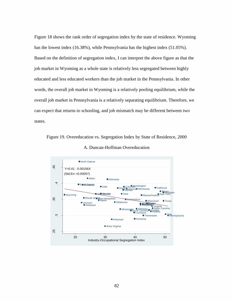
82

Figure 18 shows the rank order of segregation index by the state of residence. Wyoming

has the lowest index (16.38%), while Pennsylvania has the highest index (51.05%).

Based on the definition of segregation index, I can interpret the above figure as that the

job market in Wyoming as a whole state is relatively less segregated between highly

educated and less educated workers than the job market in the Pennsylvania. In other

words, the overall job market in Wyoming is a relatively pooling equilibrium, while the

overall job market in Pennsylvania is a relatively separating equilibrium. Therefore, we

can expect that returns to schooling, and job mismatch may be different between two

states.

Figure 19. Overeducation vs. Segregation Index by State of Residence, 2000

A. Duncan-Hoffman Overeducation

Alabama

Arizona

Arkansas

CaliforniaColorado

Connecticut

DelawareFlorida

Georgia

Idaho

Illinois

Indiana

Iowa

Kansas

Kentucky

Louisiana

Maine

Maryland

MassachusettsMichigan

Minnesota

Mississippi

Missouri

Montana

Nebraska

Nevada

New Hampshire

New Jersey

New Mexico New York

North Carolina

North Dakota

Ohio

Oklahoma

Oregon

Pennsylvania

Rhode Island

South Carolina

South Dakota

Tennessee

Texas

Utah

Vermont

Virginia

Washington

West Virginia

Wisconsin

Wyoming

Y=0.41 - 0.00156X

(Std.Err.=0.00057)

.25

.3.3

5.4

.45

Dun

can

-Ho

ffm

an

Ove

red

uca

tion

20 30 40 50Industry-Occupational Segregation Index

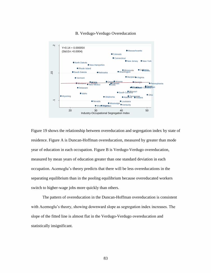
83

B. Verdugo-Verdugo Overeducation

Figure 19 shows the relationship between overeducation and segregation index by state of

residence. Figure A is Duncan-Hoffman overeducation, measured by greater than mode

year of education in each occupation. Figure B is Verdugo-Verdugo overeducation,

measured by mean years of education greater than one standard deviation in each

occupation. Acemoglu’s theory predicts that there will be less overeducations in the

separating equilibrium than in the pooling equilibrium because overeducated workers

switch to higher-wage jobs more quickly than others.

The pattern of overeducation in the Duncan-Hoffman overeducation is consistent

with Acemoglu’s theory, showing downward slope as segregation index increases. The

slope of the fitted line is almost flat in the Verdugo-Verdugo overeducation and

statistically insignificant.

Alabama

Arizona

Arkansas

California

Colorado

Connecticut

Delaware Florida

Georgia

Idaho

Illinois

Indiana

IowaKansas

Kentucky

Louisiana

Maine

Maryland

Massachusetts

Michigan

Minnesota

Mississippi

Missouri

Montana

Nebraska

Nevada

New Hampshire

New Jersey

New Mexico

New York

North Carolina

North Dakota

OhioOklahoma

OregonPennsylvania

Rhode Island

South Carolina

South Dakota

Tennessee

Texas

Utah

Vermont Virginia

Washington

West Virginia

Wisconsin

Wyoming

Y=0.14 + 0.00005X

(Std.Err.=0.0004).1

.15

.2

Ve

rdu

go

-Verd

ug

o O

vere

du

catio

n

20 30 40 50Industry-Occupational Segregation Index

84

Figure 20. Overeducation vs. College Population by State of Residence, 2000

A. Duncan-Hoffman Overeducation

B. Verdugo-Verdugo Overeducation

Alabama

Arizona

Arkansas

California Colorado

Connecticut

DelawareFlorida

Georgia

Idaho

Illinois

Indiana

Iowa

Kansas

Kentucky

Louisiana

Maine

Maryland

MassachusettsMichigan

Minnesota

Mississippi

Missouri

Montana

Nebraska

Nevada

New Hampshire

New Jersey

New Mexico New York

North Carolina

North Dakota

Ohio

Oklahoma

Oregon

Pennsylvania

Rhode Island

South Carolina

South Dakota

Tennessee

Texas

Utah

Vermont

Virginia

Washington

West Virginia

Wisconsin

Wyoming

Y=0.312 + 0.1588X

(Std.Err.=0.0832)

.25

.3.3

5.4

.45

Dun

can

-Ho

ffm

an

Ove

red

uca

tion

.1 .2 .3 .4Population of College & More Educated

Alabama

Arizona

Arkansas

California

Colorado

Connecticut

DelawareFlorida

Georgia

Idaho

Illinois

Indiana

IowaKansas

Kentucky

Louisiana

Maine

Maryland

Massachusetts

Michigan

Minnesota

Mississippi

Missouri

Montana

Nebraska

Nevada

New Hampshire

New Jersey

New Mexico

New York

North Carolina

North Dakota

OhioOklahoma

OregonPennsylvania

Rhode Island

South Carolina

South Dakota

Tennessee

Texas

Utah

VermontVirginia

Washington

West Virginia

Wisconsin

Wyoming

Y=0.045 + 0.346X

(Std.Err.=0.0270)

.1.1

5.2

Ve

rdu

go

-Verd

ug

o O

vere

du

catio

n

.1 .2 .3 .4Population of College & More Educated

85

Figure 20 shows the relationship between overeducation and population with college and

higher education by state of residence. Coefficients of both Duncan-Hoffman and

Verdugo-Verdugo measurements are statistically significant. Especially, Verdugo-

Verdugo measurement shows an almost linear relationship between overeducation and

population with college and higher education. It appears as that states with more

population with higher education are more likely to have higher overeducation.

Table 5. Duncan-Hoffman Overeducation by Occupations, 2000

Overeducation-Most Overeducation-Least

1 Transportation ticket and reservation agents Subject instructors (HS/college)

2 Kindergarten and earlier school teachers Psychologists

3 Engineering technicians Social scientists

4 Administrative support jobs Protective services

5 Insurance adjusters, examiners, and investigators Medical scientists

6 Precision makers, repairers, and smiths Physical scientists

7 Office supervisors Physicists and astronomers

8 Managers of properties and real estate Speech therapists

9 Recreation workers Photographers

10 Aircraft mechanics Vocational and educational counselors

11 Chemical technicians Broadcast equipment operators

12 Library assistants Special education teachers

13 Supervisors of personal service jobs Buyers, wholesale and retail trade

14 Computer and peripheral equipment operators Announcers

15 Surveyors, cartographers, mapping scientists and

technicians

Lawyers

16 Teachers Legal assistants, paralegals, legal support

17 Construction inspectors Advertising and related sales jobs

86

18 Other science technicians Designers

19 Customer service reps, investigators and adjusters,

except insurance

Police, detectives, and private

investigators

20 Material recording, scheduling, production,

planning, and expediting clerks

Insurance sales occupations

Table 5 shows the 20 most overeducated occupations and 20 least overeducated

occupations out of 300 occupations. Overeducation is measured based on Duncan-

Hoffman mode year of education in each occupation. According to Table 5, the

occupation of ‘Transportation Ticket and Reservation Agents’ is the most overeducated

occupation, while ‘Subject Instructors (HS/College)’ is the least overeducated occupation

for year-round full-time U.S. born workers. Overeducation is a relative concept

geographically. A worker with a required education in a region can be overeducated in a

different region, even in the same industry-occupation. If there is no physical barrier

between labor markets, however, workers will migrate to find a well-matched job as long

as benefit is higher than moving costs.

Table 6. Duncan-Hoffman Undereducation by Occupations, 2000

Undereducation-Most Undereducation-Least

1 Legal assistants, paralegals, legal support Library assistants

2 Police, detectives, and private investigators Statistical clerks

3 Art/entertainment performers and related Freight, stock, and materials handlers

4 Photographers Motion picture projectionists

5 Broadcast equipment operators Purchasing agents and buyers, of farm

products

6 Buyers, wholesale and retail trade Transportation ticket and reservation

agents

87

7 Vocational and educational counselors Insurance adjusters, examiners, and

investigators

8 Insurance sales occupations Power plant operators

9 Social scientists Interviewers, enumerators, and surveyors

10 Real estate sales occupations Computer and peripheral equipment

operators

11 Salespersons Secretaries

12 Purchasing managers, agents and buyers Other plant and system operators

13 Managers in education and related fields Payroll and timekeeping clerks

14 Management support occupations Administrative support jobs

15 Designers Bank tellers

16 Announcers Dental assistants

17 Physical scientists Typists

18 Biological technicians Patternmakers and model makers

19 Managers and administrators Correspondence and order clerks

20 Insurance underwriters Office supervisors

Table 6 shows the 20 most undereducated occupations and 20 least undereducated

occupations out of 300 occupations. Undereducation is measured based on Duncan-

Hoffman mode year of education in each occupation. According to the table 6, ‘Legal

Assistants’ is the most undereducated occupation, while ‘Library Assistants’ is the least

undereducated occupation for year-round full-time U.S. born workers.

88

2. Empirical Specification

Empirical specification analyzes wage effects of industry-occupational

segregation and job mismatch. I use a simple OLS wage equation, including segregation

index, mismatch, and interaction terms. Duncan segregation index applied in this

regression is the industry-occupational segregation at the state level.

𝐥𝐧(𝒘𝒂𝒈𝒆) = 𝜶 + 𝜷𝟏(𝑺𝒆𝒈𝒓𝒆𝒈𝒂𝒕𝒊𝒐𝒏)

+ 𝜷𝟐(𝑶𝒗𝒆𝒓 𝒆𝒅𝒖𝒄𝒂𝒕𝒊𝒐𝒏) + 𝜷𝟑(𝑼𝒏𝒅𝒆𝒓 𝒆𝒅𝒖𝒄𝒂𝒕𝒊𝒐𝒏)

+ 𝜷𝟒(𝑺𝒆𝒈𝒓𝒆𝒈𝒂𝒕𝒊𝒐𝒏 ∗ 𝑶𝒗𝒆𝒓 𝒆𝒅𝒖𝒄𝒂𝒕𝒊𝒐𝒏)

+ 𝜷𝟓(𝑺𝒆𝒈𝒓𝒆𝒈𝒂𝒕𝒊𝒐𝒏 ∗ 𝑼𝒏𝒅𝒆𝒓 𝒆𝒅𝒖𝒄𝒂𝒕𝒊𝒐𝒏) + 𝚽𝒊𝚭𝒊 + 𝜺𝒊

Acemoglu’s theory predicts that when skilled workers are abundant, employers react to

that supply by creating separate jobs for the skilled and the unskilled. Employers make

investments in capital for the skilled workers to improve productivity and thus to get

more profits, while depressing wage for unskilled workers. Therefore, as labor markets

are segregated between skilled and unskilled workers, average wage rate will increase

more than in the pooling equilibrium. Beta 1 captures the effect of occupational

segregation on wage rate. Beta 2 and Beta 3 capture wage penalty from mismatch. Their

sign and magnitude depend on mismatch measurements whether it is Duncan-Hoffman

mismatch or Verdugo-Verdugo mismatch.

Marginal effects of segregation are measured by the partial derivative

89

𝝏 𝐥𝐧 (𝒘𝒂𝒈𝒆)

𝝏 𝑺𝒆𝒈𝒓𝒆𝒈𝒂𝒕𝒊𝒐𝒏= 𝜷𝟏 + 𝜷𝟒 𝑶𝒗𝒆𝒓𝒆𝒅𝒖𝒄𝒂𝒕𝒊𝒐𝒏 + 𝜷𝟓 𝑼𝒏𝒅𝒆𝒓𝒆𝒅𝒖𝒄𝒂𝒕𝒊𝒐𝒏

𝑯𝒚𝒑𝒐𝒕𝒉𝒆𝒔𝒊𝒔 𝟏: 𝝏 𝐥𝐧 (𝒘𝒂𝒈𝒆)

𝝏 𝑺𝒆𝒈𝒓𝒆𝒈𝒂𝒕𝒊𝒐𝒏> 𝟎

Beta 4 and Beta 5 are interaction term between segregation indexes and mismatch

measurements. The purpose of interaction term is to see how labor market segregation

effects on wage in the relation with mismatch. In other words, it will tell us whether the

wage penalty is higher or lower in highly segregated labor market. I hypothesize that

overall marginal effect of segregation on wage is positive in the full specification.

Ζ𝑖 is a vector of covariates including, marital status (married with spouse

present=1, otherwise=0), four racial dummies (White non-Hispanic, Black non-Hispanic,

Asian non-Hispanic, Hispanic), five education dummies (High school=0, less than high

school, some college, college, more than college), labor market experiences (=age-

education-6, experience squared, tripled, quadrupled), four geographical dummies by

census region (Northeast=0, Midwest, South, West), metropolitan status (in metro=1,

otherwise=0) and six occupational dummies (precision or operator=0, managerial,

professional, technical, service based on OCC1990 broad occupation category in the

IPUMS-USA).

Because I use individual level data and the Segregation variable is defined based

on state, OLS standard errors should not be used because they do not account for intra-

cluster correlation. Therefore, I report standard errors clustered by state.

90

3. Results

3-1. Wage Effects of Industry-Occupational Segregation & Mismatch

Regressions were run with three different specifications for only male samples.

Specification 1:

𝐥𝐧(𝒘𝒂𝒈𝒆) = 𝜶 + 𝜷𝟏(𝑺𝒆𝒈𝒓𝒆𝒈𝒂𝒕𝒊𝒐𝒏) + 𝚽𝒊𝚭𝒊 + 𝜺𝒊

Specification 1 includes segregation index with covariates.

Specification 2:

𝐥𝐧(𝒘𝒂𝒈𝒆)

= 𝜶 + 𝜷𝟏(𝑺𝒆𝒈𝒓𝒆𝒈𝒂𝒕𝒊𝒐𝒏)

+ 𝜷𝟐(𝑶𝒗𝒆𝒓 𝒆𝒅𝒖𝒄𝒂𝒕𝒊𝒐𝒏) + 𝜷𝟑(𝑼𝒏𝒅𝒆𝒓 𝒆𝒅𝒖𝒄𝒂𝒕𝒊𝒐𝒏) + 𝚽𝒊𝚭𝒊 + 𝜺𝒊

Specification 2 includes segregation index with covariates and two mismatch

measurements: Duncan-Hoffman mismatch and Verdugo-Verdugo mismatch.

Specification 3:

𝐥𝐧(𝒘𝒂𝒈𝒆) = 𝜶 + 𝜷𝟏(𝑺𝒆𝒈𝒓𝒆𝒈𝒂𝒕𝒊𝒐𝒏)

+ 𝜷𝟐(𝑶𝒗𝒆𝒓 𝒆𝒅𝒖𝒄𝒂𝒕𝒊𝒐𝒏) + 𝜷𝟑(𝑼𝒏𝒅𝒆𝒓 𝒆𝒅𝒖𝒄𝒂𝒕𝒊𝒐𝒏)

+ 𝜷𝟒(𝑺𝒆𝒈𝒓𝒆𝒈𝒂𝒕𝒊𝒐𝒏 ∗ 𝑶𝒗𝒆𝒓 𝒆𝒅𝒖𝒄𝒂𝒕𝒊𝒐𝒏)

+ 𝜷𝟓(𝑺𝒆𝒈𝒓𝒆𝒈𝒂𝒕𝒊𝒐𝒏 ∗ 𝑼𝒏𝒅𝒆𝒓 𝒆𝒅𝒖𝒄𝒂𝒕𝒊𝒐𝒏) + 𝚽𝒊𝚭𝒊 + 𝜺𝒊

Specification 3 is a full specification, which includes segregation index,

mismatch, interaction term between mismatch and segregation index, and covariates.

Covariates in the each regression are marital status dummy, four racial dummies,

five education dummies, labor market experiences, four regional dummies, metropolitan

91

status dummy, and six occupational dummies. The dependent variable is log weekly

wage converted to 1999 constant dollar value.

92

Table 7. Specification (1) for Wage Effects of Industry-Occupational Segregation

Dependent Variable is Log Weekly Wage ($1999)

1960 1970 1980 1990 2000

Segregation Index 0.00165 0.00202 0.00230 0.00576*** 0.00286*

(0.00150) (0.00187) (0.00141) (0.00206) (0.00165)

Covariates Y Y Y Y Y

Mismatch Variables N N N N N

Observations 108228 114897 636312 822145 847385

R-squared 0.360 0.390 0.363 0.388 0.377

* p<0.10, ** p<0.05, *** p<0.01, Regression is for males.

93

Table 7 is the regression result of wage effects of industry-occupational segregation by

regression specification (1). The specification (1) is the simplest specification and

includes segregation index, covariates but excludes mismatch variables, purposing isolate

wage effects of segregation from wage effects of job mismatch.

Table 7 reveals that average wage rate is higher in states where industry-

occupations are more separated between skilled (college and more educated) and

unskilled workers (less than college educated). The magnitudes of coefficient are

increasing up to 1990 and decreased in 2000, but coefficients are statistically significant

for 2000 and 1990 only.

94

Table 8. Specification (2) for Wage Effects of Industry-Occupational Segregation

A. Duncan-Hoffman Mismatch

Dependent Variable is Log Weekly Wage ($1999)

1960 1970 1980 1990 2000

Segregation Index 0.00158 0.00192 0.00228 0.00574*** 0.00282*

(0.00140) (0.00184) (0.00140) (0.00206) (0.00164)

Years of Over education 0.04419*** 0.04321*** 0.02376*** 0.02629*** 0.01293***

(0.00301) (0.00276) (0.00154) (0.00138) (0.00119)

Years of Under education -0.03653*** -0.02664*** -0.02679*** -0.03041*** -0.02884***

(0.00248) (0.00214) (0.00149) (0.00125) (0.00116)

Years of Required education 0.04710*** 0.02126*** 0.02166*** 0.07381*** 0.07206***

(0.00293) (0.00465) (0.00344) (0.00204) (0.00145)

Covariates Y Y Y Y Y

Observations 108228 114897 636312 822145 847385

R-squared 0.373 0.396 0.366 0.395 0.388

* p<0.10, ** p<0.05, *** p<0.01, Regression is for males.

95

B. Verdugo-Verdugo Mismatch

Dependent Variable is Log Weekly Wage ($1999)

1960 1970 1980 1990 2000

Segregation Index 0.00165 0.00201 0.00230 0.00576*** 0.00285*

(0.00150) (0.00187) (0.00141) (0.00206) (0.00164)

Over education -0.02581*** -0.00883 -0.01995*** -0.05812*** -0.06606***

(0.00566) (0.00583) (0.00484) (0.00534) (0.00637)

Under education -0.03729*** -0.01635* -0.02302*** 0.03694*** 0.07127***

(0.01354) (0.00892) (0.00542) (0.00522) (0.00604)

Covariates Y Y Y Y Y

Observations 108228 114897 636312 822145 847385

R-squared 0.361 0.390 0.364 0.389 0.378

* p<0.10, ** p<0.05, *** p<0.01, Regression is for males.

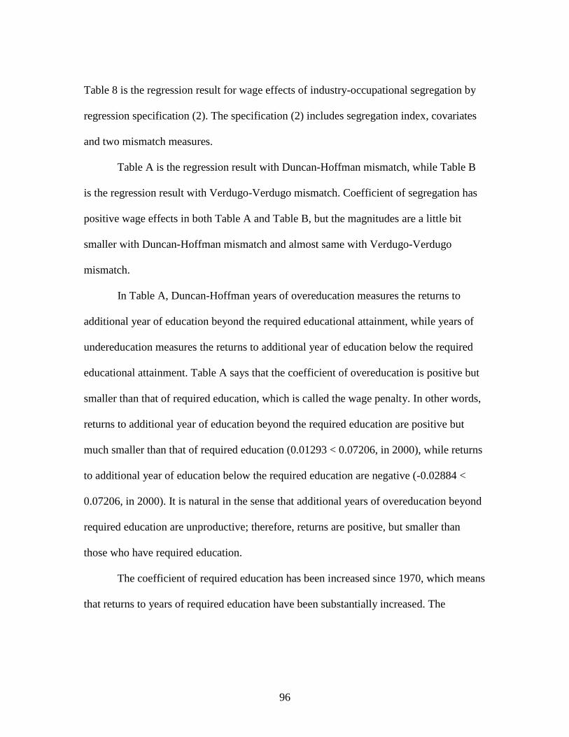
96

Table 8 is the regression result for wage effects of industry-occupational segregation by

regression specification (2). The specification (2) includes segregation index, covariates

and two mismatch measures.

Table A is the regression result with Duncan-Hoffman mismatch, while Table B

is the regression result with Verdugo-Verdugo mismatch. Coefficient of segregation has

positive wage effects in both Table A and Table B, but the magnitudes are a little bit

smaller with Duncan-Hoffman mismatch and almost same with Verdugo-Verdugo

mismatch.

In Table A, Duncan-Hoffman years of overeducation measures the returns to

additional year of education beyond the required educational attainment, while years of

undereducation measures the returns to additional year of education below the required

educational attainment. Table A says that the coefficient of overeducation is positive but

smaller than that of required education, which is called the wage penalty. In other words,

returns to additional year of education beyond the required education are positive but

much smaller than that of required education (0.01293 < 0.07206, in 2000), while returns

to additional year of education below the required education are negative (-0.02884 <

0.07206, in 2000). It is natural in the sense that additional years of overeducation beyond

required education are unproductive; therefore, returns are positive, but smaller than

those who have required education.

The coefficient of required education has been increased since 1970, which means

that returns to years of required education have been substantially increased. The

97

coefficient of overeducation has been decreased since 1960, which means that wage

penalty for holding an additional year of education has been substantially increased.

Table B is the regression result with Verdugo-Verdugo mismatch. Overeducation

and undereducation are dummy variables in the Verdugo-Verdugo mismatch. In Table B,

the coefficient of overeducation is negative (which is called wage penalty) and the

coefficient of undereducation is positive (which is called substantial wage premium),

which is consistent with empirical findings from previous literatures. It tells us that,

relative to workers who have required education, wage penalty related with

overeducation is substantially higher. The coefficient of undereducation is positive only

in 1990, 2000, which there are wage premiums related with undereducation. Absolute

value of coefficient of overeducation has been increased since 1970, which means that

wage penalty from overeducation has been substantially increased.

98

Table 9. Specification (3) for Wage Effects of Industry-Occupational Segregation.

A. Duncan-Hoffman Mismatch

Dependent Variable is Log Weekly Wage ($1999)

1960 1970 1980 1990 2000

Segregation Index -0.00428 -0.01073* -0.00973* -0.00544 -0.00707*

(0.00310) (0.00633) (0.00518) (0.00434) (0.00398)

Years of Over education 0.04134*** 0.00392 -0.00754 -0.02808*** -0.02654**

(0.01402) (0.02080) (0.01037) (0.01037) (0.01045)

Segregation*Years of Over education 0.00006 0.00081* 0.00075*** 0.00129*** 0.00089***

(0.00031) (0.00042) (0.00026) (0.00024) (0.00023)

Years of Under education -0.05459*** -0.04710*** -0.04269*** -0.03089*** -0.02323***

(0.01106) (0.01356) (0.00933) (0.01054) (0.00757)

Segregation*Years of Under education 0.00039 0.00043 0.00038* 0.00001 -0.00013

(0.00025) (0.00029) (0.00022) (0.00025) (0.00017)

Years of Required education 0.02639** -0.02441 -0.01579 0.04047*** 0.04048***

(0.01181) (0.02544) (0.01568) (0.01437) (0.01486)

Segregation*Years of Required education 0.00043* 0.00094* 0.00089** 0.00079** 0.00071**

(0.00025) (0.00054) (0.00041) (0.00035) (0.00034)

Covariates Y Y Y Y Y

Observations 108228 114897 636312 822145 847385

R-squared 0.374 0.396 0.367 0.395 0.388

* p<0.10, ** p<0.05, *** p<0.01, Regression is for males.

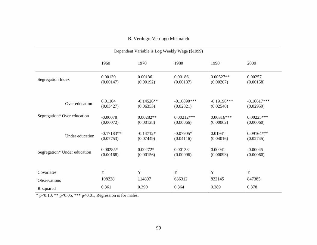
99

B. Verdugo-Verdugo Mismatch

Dependent Variable is Log Weekly Wage ($1999)

1960 1970 1980 1990 2000

Segregation Index 0.00139 0.00136 0.00186 0.00527** 0.00257

(0.00147) (0.00192) (0.00137) (0.00207) (0.00158)

Over education 0.01104 -0.14526** -0.10890*** -0.19196*** -0.16617***

(0.03427) (0.06353) (0.02821) (0.02540) (0.02959)

Segregation* Over education -0.00078 0.00282** 0.00212*** 0.00316*** 0.00225***

(0.00072) (0.00128) (0.00066) (0.00062) (0.00060)

Under education -0.17183** -0.14712* -0.07905* 0.01941 0.09164***

(0.07753) (0.07449) (0.04116) (0.04016) (0.02745)

Segregation* Under education 0.00285* 0.00272* 0.00133 0.00041 -0.00045

(0.00168) (0.00156) (0.00096) (0.00093) (0.00060)

Covariates Y Y Y Y Y

Observations 108228 114897 636312 822145 847385

R-squared 0.361 0.390 0.364 0.389 0.378

* p<0.10, ** p<0.05, *** p<0.01, Regression is for males.

100

Table 9 is the regression result of wage effects of industry-occupational segregation by

regression specification (3), which is a full specification, including segregation index,

covariates, mismatch measures, and interaction term between mismatch and segregation

index. The purpose of interaction term is purpose to see the wage effects of mismatch in

relation with segregation. Table A is with Duncan-Hoffman mismatch, and Table B is

with Verdugo-Verdugo mismatch.

Marginal effect of segregation from Duncan-Hoffman Mismatch for 2000 is

expressed as follows with coefficients from Table A.

𝝏 𝐥𝐧 (𝒘𝒂𝒈𝒆)

𝝏 𝑺𝒆𝒈𝒓𝒆𝒈𝒂𝒕𝒊𝒐𝒏

= −𝟎. 𝟎𝟎𝟕 + 𝟎. 𝟎𝟎𝟎𝟖𝟗(𝒚𝒆𝒂𝒓𝒔 𝒐𝒇 𝒐𝒗𝒆𝒓𝒆𝒅𝒖𝒄𝒂𝒕𝒊𝒐𝒏)

− 𝟎. 𝟎𝟎𝟎𝟏𝟑(𝒚𝒆𝒂𝒓𝒔 𝒐𝒇 𝒖𝒏𝒅𝒆𝒓𝒆𝒅𝒖𝒄𝒂𝒕𝒊𝒐𝒏)

+ 𝟎. 𝟎𝟎𝟎𝟕𝟏(𝒚𝒆𝒂𝒓𝒔 𝒐𝒇 𝒓𝒆𝒒𝒖𝒊𝒓𝒆𝒅 𝒆𝒅𝒖𝒄𝒂𝒕𝒊𝒐𝒏)

With the mean value of years of overeducation, years of undereducation, and years of

required education from the summary statistics table, marginal effect of segregation is

calculated as follows

𝝏 𝐥𝐧 (𝒘𝒂𝒈𝒆)

𝝏 𝑺𝒆𝒈𝒓𝒆𝒈𝒂𝒕𝒊𝒐𝒏= −𝟎. 𝟎𝟎𝟕 + 𝟎. 𝟎𝟎𝟎𝟖𝟗(𝟎. 𝟓𝟗) − 𝟎. 𝟎𝟎𝟎𝟏𝟑(−𝟎. 𝟓𝟖) + 𝟎. 𝟎𝟎𝟎𝟕𝟏(𝟏𝟑. 𝟑𝟖)

= 𝟎. 𝟎𝟎𝟑𝟏 > 𝟎

I can see the positive effect of segregation and it can be interpreted as a partial elasticity.

Weekly wage will increase 0.31% to one unit increase in segregation index at the mean.

101

The wage effects of years of overeducation, years of undereducation, and years of

required education in the relation with segregation for 2000 can be calculated as follows,

respectively

𝝏 𝐥𝐧 (𝒘𝒂𝒈𝒆)

𝝏 𝒚𝒆𝒂𝒓𝒔 𝒐𝒇 𝒐𝒗𝒆𝒓𝒆𝒅𝒖𝒄𝒂𝒕𝒊𝒐𝒏= −𝟎. 𝟎𝟐𝟔𝟓𝟒 + 𝟎. 𝟎𝟎𝟎𝟖𝟗(𝒔𝒆𝒈𝒓𝒆𝒈𝒂𝒕𝒊𝒐𝒏)

𝝏 𝐥𝐧 (𝒘𝒂𝒈𝒆)

𝝏 𝒚𝒆𝒂𝒓𝒔 𝒐𝒇 𝒖𝒏𝒅𝒆𝒓𝒆𝒅𝒖𝒄𝒂𝒕𝒊𝒐𝒏= −𝟎. 𝟎𝟐𝟑𝟐𝟑 − 𝟎. 𝟎𝟎𝟎𝟏𝟑(𝒔𝒆𝒈𝒓𝒆𝒈𝒂𝒕𝒊𝒐𝒏)

𝝏 𝐥𝐧 (𝒘𝒂𝒈𝒆)

𝝏 𝒚𝒆𝒂𝒓𝒔 𝒐𝒇 𝒓𝒆𝒒𝒖𝒊𝒓𝒆𝒅 𝒆𝒅𝒖𝒄𝒂𝒕𝒊𝒐𝒏= 𝟎. 𝟎𝟒𝟎𝟒𝟖 + 𝟎. 𝟎𝟎𝟎𝟕𝟏(𝒔𝒆𝒈𝒓𝒆𝒈𝒂𝒕𝒊𝒐𝒏)

It tells us that first, returns to years of education is higher for those who have required

education and followed by for those who have overeducation. The second finding is that

returns to additional years of overeducation beyond (below) the required education are

decreasing but such wage penalty becomes smaller (larger) in the state where industry-

occupations are more separated between the skilled and the unskilled. In other words,

wage penalty related with overeducation is substantially higher but it becomes smaller in

the states where industry-occupations are more separated between the skilled and the

unskilled. As Acemoglu’s theory predicts, skilled workers earn more and unskilled

workers earn less in the separating equilibrium because overeducation is a matter to the

skilled workers generally.

Marginal effects of segregation from Verdugo-Verdugo Mismatch for 2000 is as

follows:

102

𝝏 𝐥𝐧 (𝒘𝒂𝒈𝒆)

𝝏 𝑺𝒆𝒈𝒓𝒆𝒈𝒂𝒕𝒊𝒐𝒏= 𝟎. 𝟎𝟎𝟐𝟓𝟕 + 𝟎. 𝟎𝟎𝟐𝟐𝟓(𝒐𝒗𝒆𝒓 𝒆𝒅𝒖𝒄𝒂𝒕𝒊𝒐𝒏) − 𝟎. 𝟎𝟎𝟎𝟒𝟓(𝒖𝒏𝒅𝒆𝒓 𝒆𝒅𝒖𝒄𝒂𝒕𝒊𝒐𝒏)

Verdugo-Verdugo mismatch is dummy variable with using required education as a

reference category. Therefore, in the above marginal effects of segregation,

overeducation and undereducation cannot be equal to 1 at the same time. Marginal effects

of segregation is 0.00482 if overeducation=1, while it is 0.00212 if undereducation=1. In

either case, marginal effects of segregation are positive.

The wage effects of overeducation and undereducation in the relation with

segregation for 2000 can be calculated as follows, respectively.

𝝏 𝐥𝐧 (𝒘𝒂𝒈𝒆)

𝝏 𝒐𝒗𝒆𝒓𝒆𝒅𝒖𝒄𝒂𝒕𝒊𝒐𝒏= −𝟎. 𝟏𝟔𝟔𝟏𝟕 + 𝟎. 𝟎𝟎𝟐𝟐𝟓(𝒔𝒆𝒈𝒓𝒆𝒈𝒂𝒕𝒊𝒐𝒏), 𝒊𝒇 𝒐𝒗𝒆𝒓𝒆𝒅𝒖𝒄𝒂𝒕𝒊𝒐𝒏 = 𝟏

𝝏 𝐥𝐧 (𝒘𝒂𝒈𝒆)

𝝏 𝒖𝒏𝒅𝒆𝒓𝒆𝒅𝒖𝒄𝒂𝒕𝒊𝒐𝒏= 𝟎. 𝟎𝟗𝟏𝟔𝟒 − 𝟎. 𝟎𝟎𝟎𝟒𝟓(𝒔𝒆𝒈𝒓𝒆𝒈𝒂𝒕𝒊𝒐𝒏), 𝒊𝒇 𝒖𝒏𝒅𝒆𝒓𝒆𝒅𝒖𝒄𝒂𝒕𝒊𝒐𝒏 = 𝟏

The wage effects of overeducation (undereducation) reveal that workers who are

overeducated (undereducated) obtain less (more) than workers who have required

education, but such wage penalty (wage premium) becomes smaller in the states where

industry-occupations are more separated between the skilled and the unskilled (second

term of right hand side). Therefore, skilled workers earn more and unskilled workers earn

less in the separating equilibrium.

In summary, three regression specifications examine the wage effects of industry-

occupational segregation and the wage effects of mismatch, and wage effects of

mismatch in the relation with industry-occupational segregation. The first finding is that

wage effects of industry-occupational segregation are positive. The second finding is that

103

the wage penalty related with overeducation is substantially high for all study periods. In

fact, the pattern of wage penalty has been increased over time. The third finding is that

the wage penalty from overeducation becomes smaller in states where industry-

occupations are more separated between skilled and unskilled workers. The fourth

finding that differs from those of previous studies is about wage effects of mismatch in

the relation with segregation because previous studies did not consider that the labor

market can transform from a pooling equilibrium to a separating equilibrium, and

accordingly, the wage penalty from overeducation also can be different in the pooling

equilibrium and in the separating equilibrium.

104

Table 10. Alternative Specification for Wage Effects of Industry-Occupational Segregation.

Dependent Variable is Log Weekly Wage ($1999)

Duncan-Hoffman Mismatch

1960 1970 1980 1990 2000

Segregation Index 0.00103 0.00086 0.00129 0.00431* 0.00199

(0.00153) (0.00198) (0.00133) (0.00221) (0.00169)

Over education 0.06623 -0.06645 -0.09081*** -0.23519*** -0.23016***

(0.04376) (0.06703) (0.02854) (0.02683) (0.01784)

Segregation*Over education -0.00080 0.00250* 0.00188*** 0.00330*** 0.00192***

(0.00092) (0.00138) (0.00064) (0.00068) (0.00039)

Under education -0.03630 -0.01683 -0.11114*** -0.05449* -0.01858

(0.05028) (0.06392) (0.03157) (0.02926) (0.02033)

Segregation*Under education 0.00175 0.00158 0.00175** 0.00171** 0.00093**

(0.00104) (0.00122) (0.00075) (0.00070) (0.00044)

Covariates Y Y Y Y Y

Observations 108228 114897 636312 822145 847385

R-squared 0.361 0.391 0.364 0.390 0.383

* p<0.10, ** p<0.05, *** p<0.01, Regression is for males.

105

In Table 10, both overeducation and undereducation are simple dummy variables from

Duncan-Hoffman mismatch, instead of measuring how many additional years of

education are overeducated or undereducated than the required education. If workers’

educational attainments are higher (lower) than the mode year of education in occupation,

they are classified to overeducation (undereducation).

Marginal effects of segregation for 2000 is expressed as follow

𝝏 𝐥𝐧 (𝒘𝒂𝒈𝒆)

𝝏 𝑺𝒆𝒈𝒓𝒆𝒈𝒂𝒕𝒊𝒐𝒏= 𝟎. 𝟎𝟎𝟏𝟗𝟗 + 𝟎. 𝟎𝟎𝟏𝟗𝟐(𝒐𝒗𝒆𝒓 𝒆𝒅𝒖𝒄𝒂𝒕𝒊𝒐𝒏) + 𝟎. 𝟎𝟎𝟎𝟗𝟑(𝒖𝒏𝒅𝒆𝒓 𝒆𝒅𝒖𝒄𝒂𝒕𝒊𝒐𝒏)

Required education is a reference category. Therefore, in the above marginal effects of

segregation, overeducation and undereducation cannot be equal to 1 at the same time.

Either of case, however, marginal effects of segregation is positive.

The wage effects of overeducation and undereducation in the relation with

segregation for 2000 can be calculated as follows, respectively:

𝝏 𝐥𝐧 (𝒘𝒂𝒈𝒆)

𝝏 𝒐𝒗𝒆𝒓𝒆𝒅𝒖𝒄𝒂𝒕𝒊𝒐𝒏= −𝟎. 𝟐𝟑𝟎𝟏𝟔 + 𝟎. 𝟎𝟎𝟏𝟗𝟐(𝒔𝒆𝒈𝒓𝒆𝒈𝒂𝒕𝒊𝒐𝒏), 𝒊𝒇 𝒐𝒗𝒆𝒓𝒆𝒅𝒖𝒄𝒂𝒕𝒊𝒐𝒏 = 𝟏

𝝏 𝐥𝐧 (𝒘𝒂𝒈𝒆)

𝝏 𝒖𝒏𝒅𝒆𝒓𝒆𝒅𝒖𝒄𝒂𝒕𝒊𝒐𝒏= −𝟎. 𝟎𝟏𝟖𝟓𝟖 + 𝟎. 𝟎𝟎𝟎𝟗𝟑(𝒔𝒆𝒈𝒓𝒆𝒈𝒂𝒕𝒊𝒐𝒏), 𝒊𝒇 𝒖𝒏𝒅𝒆𝒓𝒆𝒅𝒖𝒄𝒂𝒕𝒊𝒐𝒏 = 𝟏

Wage penalty for both overeducation and undereducation is substantially large but

it becomes smaller in states where industry-occupations are more separated between

skilled and unskilled workers. I can find the same results that marginal effects of

segregation is positive and wage penalty related with overeducation becomes smaller in

106

the states where industry-occupations are more separated between skilled and unskilled

workers.

3-2. College Wage Premiums

This section examines changes in the college wage premium over time, using five

educational categories and use high school graduates as a reference category. Following

is the regression specification.

𝒍𝒏(𝑾𝒂𝒈𝒆)

= 𝜶𝟏 + 𝜷𝟏(𝑬𝒅𝒖𝒊)

+ 𝜷𝟐(𝑺𝒆𝒈𝒓𝒆𝒈𝒂𝒕𝒊𝒐𝒏)

+ 𝜷3(𝑪𝒐𝒍𝒍𝒆𝒈𝒆 ∗ 𝑺𝒆𝒈𝒓𝒆𝒈𝒂𝒕𝒊𝒐𝒏)

+ 𝜷𝟒(𝑶𝒗𝒆𝒓𝒆𝒅𝒖𝒄𝒂𝒕𝒊𝒐𝒏) + 𝜷5(𝑼𝒏𝒅𝒆𝒓𝒆𝒅𝒖𝒄𝒂𝒕𝒊𝒐𝒏) + 𝜱𝒊𝜡𝒊 + 𝜺𝒊

𝑯𝒚𝒑𝒐𝒕𝒉𝒆𝒔𝒊𝒔: 𝜷𝟑 > 𝟎

Relative college wage premiums are higher in states where industry-occupations

are more separated between skilled and unskilled workers as Acemoglu’s theory predicts.

Marginal effects of college in the relation with segregation are measured by the partial

derivative as follows:

𝝏 𝐥𝐧 (𝒘𝒂𝒈𝒆)

𝝏 𝑪𝒐𝒍𝒍𝒆𝒈𝒆= 𝜷𝟏 + 𝜷𝟑 𝑺𝒆𝒈𝒓𝒆𝒈𝒂𝒕𝒊𝒐𝒏

Regressions were run with three different specifications for only male samples.

107

Specification (1):

𝒍𝒏(𝑾𝒂𝒈𝒆) = 𝜶𝟏 + 𝜷𝟏(𝑬𝒅𝒖𝒊) + 𝜱𝒊𝜡𝒊 + 𝜺𝒊

Specification (1) includes educational dummies and covariates.

Specification (2):

𝒍𝒏(𝑾𝒂𝒈𝒆)

= 𝜶𝟏 + 𝜷𝟏(𝑬𝒅𝒖𝒊)

+ 𝜷𝟐(𝑺𝒆𝒈𝒓𝒆𝒈𝒂𝒕𝒊𝒐𝒏)

+ 𝜷𝟑(𝑶𝒗𝒆𝒓𝒆𝒅𝒖𝒄𝒂𝒕𝒊𝒐𝒏) + 𝜷𝟒(𝑼𝒏𝒅𝒆𝒓𝒆𝒅𝒖𝒄𝒂𝒕𝒊𝒐𝒏) + 𝜱𝒊𝜡𝒊 + 𝜺𝒊

Specification (2) includes educational dummies, industry-occupational

segregation index, mismatch variables, and covariates.

Specification (3):

𝒍𝒏(𝑾𝒂𝒈𝒆)

= 𝜶𝟏 + 𝜷𝟏(𝑬𝒅𝒖𝒊)

+ 𝜷𝟐(𝑺𝒆𝒈𝒓𝒆𝒈𝒂𝒕𝒊𝒐𝒏)

+ 𝜷𝟑(𝑪𝒐𝒍𝒍𝒆𝒈𝒆 ∗ 𝑺𝒆𝒈𝒓𝒆𝒈𝒂𝒕𝒊𝒐𝒏) + 𝜷𝟒(𝑶𝒗𝒆𝒓𝒆𝒅𝒖𝒄𝒂𝒕𝒊𝒐𝒏)

+ 𝜷𝟓(𝑼𝒏𝒅𝒆𝒓𝒆𝒅𝒖𝒄𝒂𝒕𝒊𝒐𝒏) + 𝜱𝒊𝜡𝒊 + 𝜺𝒊

Specification (3) is a full specification which includes educational dummies,

industry-occupational segregation index, mismatch variables, interaction term between

college and segregation index, and covariates. The purpose of the interaction term is to

see college wage premiums in the relation with industry-occupational segregation.

108

Table 11. Specification (1) for College Wage Premiums

Dependent Variable is Log Weekly Wage ($1999)

1960 1970 1980 1990 2000

College 0.27396*** 0.32963*** 0.28433*** 0.40537*** 0.38542***

(0.01053) (0.01313) (0.00761) (0.00767) (0.00765)

Less than High School -0.13525*** -0.17021*** -0.14393*** -0.17838*** -0.15442***

(0.00831) (0.00760) (0.00637) (0.00743) (0.00455)

Some College 0.09613*** 0.07319*** 0.09247*** 0.13699*** 0.12345***

(0.00585) (0.00698) (0.00388) (0.00534) (0.00328)

Over College 0.28697*** 0.40125*** 0.38781*** 0.56637*** 0.53022***

(0.01229) (0.02302) (0.01227) (0.00924) (0.00833)

Segregation Index N N N N N

Mismatch Variables N N N N N

Covariates Y Y Y Y Y

Observations 108228 117081 636312 822145 847385

R-squared 0.360 0.333 0.363 0.385 0.376

* p<0.10, ** p<0.05, *** p<0.01, Regression is for males.

109

Table 11 shows the regression results for college wage premiums by regression

specification (1), which includes covariates. The purpose of the specification (1) is to

isolate wage effects of college education from wage effects of job mismatch. Relative to

high school graduates, wage rate for college graduates shows variations over time. It

might reflect changes in the supply of and demand for college graduates. For 1990,

weekly college wage is about 50% ({exp(0.40537)-1}*100=49.99) higher than high

school graduates. Overall, college wage premiums are higher in 2000, 1990 than other

periods.

110

Table 12. Specification (2) for College Wage Premiums

A. Duncan-Hoffman Mismatch

Dependent Variable is Log Weekly Wage ($1999)

1960 1970 1980 1990 2000

College 0.11343*** 0.16949*** 0.19401*** 0.27838*** 0.27785***

(0.01047) (0.01425) (0.00692) (0.00872) (0.00893)

Less than High School -0.02050*** -0.07323*** -0.07158*** -0.10516*** -0.08793***

(0.00446) (0.00547) (0.00378) (0.00613) (0.00489)

Some College 0.03007*** 0.00624 0.05490*** 0.09952*** 0.10343***

(0.00381) (0.00667) (0.00342) (0.00520) (0.00340)

Over College 0.00784 0.13766*** 0.25331*** 0.36210*** 0.35866***

(0.01160) (0.02479) (0.00932) (0.01167) (0.01082)

Segregation Index 0.00158 0.00213 0.00228 0.00574*** 0.00574***

(0.00140) (0.00180) (0.00140) (0.00206) (0.00206)

Mismatch Variables Y Y Y Y Y

Covariates Y Y Y Y Y

Observations 108228 117081 636312 822145 847385

R-squared 0.373 0.340 0.366 0.395 0.388

* p<0.10, ** p<0.05, *** p<0.01, Regression is for males.

111

B. Verdugo-Verdugo Mismatch

Dependent Variable is Log Weekly Wage ($1999)

1960 1970 1980 1990 2000

College 0.28615*** 0.32971*** 0.29272*** 0.44720*** 0.44156***

(0.01059) (0.01410) (0.00854) (0.00768) (0.01092)

Less than High School -0.13468*** -0.16101*** -0.13451*** -0.20140*** -0.19904***

(0.00638) (0.00595) (0.00544) (0.00568) (0.00511)

Some College 0.09894*** 0.07354*** 0.09623*** 0.14701*** 0.13994***

(0.00531) (0.00725) (0.00389) (0.00550) (0.00340)

Over College 0.30082*** 0.40221*** 0.40278*** 0.63034*** 0.61282***

(0.01107) (0.02462) (0.01470) (0.01150) (0.01368)

Segregation Index 0.00165 0.00224 0.00230 0.00576*** 0.00285*

(0.00150) (0.00184) (0.00141) (0.00206) (0.00164)

Mismatch Variables Y Y Y Y Y

Covariates Y Y Y Y Y

Observations 108228 117081 636312 822145 847385

R-squared 0.361 0.334 0.364 0.389 0.378

* p<0.10, ** p<0.05, *** p<0.01, Regression is for males.

112

Table 12 shows the regression results for college wage premiums by regression

specification (2), which includes covariates, industry-occupational segregation index, and

mismatch variables. Table A is regression with Duncan-Hoffman mismatch, while Table

B is regression with Verdugo-Verdugo mismatch.

In Table A with Duncan-Hoffman mismatch, coefficients of college are much

smaller than in the Table 11, which has with no mismatch. Coefficients of college have

been increased with Duncan-Hoffman mismatch. In other words, relative college wage

premiums have been increased.

In Table B with Verdugo-Verdugo mismatch, coefficients of college are much

larger than in the Table 11, which has no mismatch. Coefficients of college have been

varied very much over time. No constant pattern can be found.

Overall, college wage premiums are affected with or without mismatch variables,

reflecting overeducation is mostly a matter for college graduates.

113

Table 13. Specification (3) for College Wage Premiums

A. Duncan-Hoffman Mismatch

Dependent Variable is Log Weekly Wage ($1999)

1960 1970 1980 1990 2000

College 0.10632 0.07820 0.11913** 0.15725*** 0.17345***

(0.07040) (0.09763) (0.04507) (0.04031) (0.05549)

College*Segregation 0.00015 0.00187 0.00176 0.00284*** 0.00234*

(0.00139) (0.00207) (0.00108) (0.00095) (0.00129)

Less than High School -0.02049*** -0.07318*** -0.07165*** -0.10528*** -0.08809***

(0.00445) (0.00546) (0.00378) (0.00611) (0.00487)

Some College 0.03006*** 0.00608 0.05458*** 0.09938*** 0.10327***

(0.00382) (0.00659) (0.00342) (0.00516) (0.00342)

Over College 0.00779 0.13728*** 0.25262*** 0.36177*** 0.35852***

(0.01181) (0.02461) (0.00926) (0.01164) (0.01080)

Segregation Index 0.00157 0.00199 0.00207 0.00528** 0.00241

(0.00140) (0.00179) (0.00137) (0.00204) (0.00153)

Mismatch Variables Y Y Y Y Y

Covariates Y Y Y Y Y

Observations 108228 117081 636312 822145 847385

R-squared 0.373 0.340 0.366 0.395 0.388

* p<0.10, ** p<0.05, *** p<0.01, Regression is for males.

114

B. Verdugo-Verdugo Mismatch

Dependent Variable is Log Weekly Wage ($1999)

1960 1970 1980 1990 2000

College 0.30712*** 0.25964*** 0.22362*** 0.33174*** 0.32825***

(0.07098) (0.09417) (0.04402) (0.04100) (0.05625)

College*Segregation -0.00044 0.00144 0.00164 0.00271*** 0.00254*

(0.00147) (0.00203) (0.00109) (0.00098) (0.00138)

Less than High School -0.13469*** -0.16100*** -0.13457*** -0.20151*** -0.19918***

(0.00637) (0.00595) (0.00545) (0.00566) (0.00511)

Some College 0.09894*** 0.07354*** 0.09619*** 0.14698*** 0.13987***

(0.00532) (0.00722) (0.00387) (0.00544) (0.00342)

Over College 0.30087*** 0.40233*** 0.40285*** 0.63017*** 0.61275***

(0.01107) (0.02469) (0.01471) (0.01146) (0.01367)

Segregation Index 0.00168 0.00213 0.00210 0.0532** 0.00241

(0.00150) (0.00182) (0.00138) (0.00204) (0.00152)

Mismatch Variables Y Y Y Y Y

Covariates Y Y Y Y Y

Observations 108228 117081 636312 822145 847385

R-squared 0.361 0.334 0.364 0.389 0.378

* p<0.10, ** p<0.05, *** p<0.01, Regression is for males.

115

Table 13 shows the regression results for college wage premiums by regression

specification (3), which is a full specification. Table A is regression with Duncan-

Hoffman mismatch, while Table B is regression with Verdugo-Verdugo mismatch.

Wage effects of college education are measured as follows for 2000 with Duncan-

Hoffman mismatch and Verdugo-Verdugo mismatch, respectively:

𝝏 𝐥𝐧 (𝒘𝒂𝒈𝒆)

𝝏 𝑪𝒐𝒍𝒍𝒆𝒈𝒆= 𝟎. 𝟏𝟕𝟑𝟒𝟓 + 𝟎. 𝟎𝟎𝟐𝟑𝟒(𝑺𝒆𝒈𝒓𝒆𝒈𝒂𝒕𝒊𝒐𝒏)

𝝏 𝐥𝐧 (𝒘𝒂𝒈𝒆)

𝝏 𝑪𝒐𝒍𝒍𝒆𝒈𝒆= 𝟎. 𝟑𝟐𝟖𝟐𝟓 + 𝟎. 𝟎𝟎𝟐𝟓𝟒(𝑺𝒆𝒈𝒓𝒆𝒈𝒂𝒕𝒊𝒐𝒏)

With controlling Duncan-Hoffman mismatch, the coefficient of college is much smaller

than the coefficient of controlling Verdugo-Verdugo mismatch, but the magnitudes of

coefficient of interaction term are almost the same. The coefficient of interaction term tells

us that college wage premiums increase in the states where industry-occupations are more

separated between the skilled and the unskilled. In other words, skilled workers earn more

wages in the separating equilibrium than in the pooling equilibrium.

In summary, relative to high school graduates, college wage premiums have

fluctuated over time, reflecting changes in the supply of and demand for college

graduates in the labor markets. The interaction term between the college dummy variable

and segregation index reveals that college graduates earn more in states where industry-

occupations are more separated between skilled and unskilled workers. In other words,

skilled workers earn more wages in the separating equilibrium than in the pooling

equilibrium.

116

CHAPTER SEVEN

CONCLUSION

This paper began with analyzing a cause and effect relationship between the

Soviet launch of Sputnik and educational reform in the early 1960s in the United States.

During the Cold War, the Soviet launching of Sputnik poured fuel onto an existing arms

race between the Soviets and America. The American public and government perceived

Sputnik to be more a military threat than a simple product of science education. President

Eisenhower, however, found that they had a shortfall in scientists and had a lack of

science education to compete with USSR. Therefore, educational reform was arose

immediately. First, the American government extended the role of the existing National

Science Foundation in science education and production of science elites. Second,

Eisenhower signed into law the National Defense of Education Act on September 2,

1958, which was less than a year after the launching of Sputnik 1. Congress authorized

budgets for NSF and NDEA to produce science and defense related human capitals. The

NDEA poured $887 million over four years into programs intended to develop talented

people in America in fields related with national defense by providing scholarships to

students. During the Eisenhower administration, the goal of federal funding was

producing scientists and engineers for the national security.

After Eisenhower, Kennedy became the President. His domestic agendas, under

the name of the New Frontier, were racial integration, equality of the sex in the work

place, civil rights of African American, and extending equal opportunity of access to

higher education by minority races. After Kennedy’s assassination, Lyndon Johnson

117

became the President. Johnson was interested in civil rights, eliminating poverty, and

racial injustice under his domestic program, Great Society. The Higher Education Act

was signed into law in 1965, and was one of the fruits of Great Society. Sputnik-triggered

educational reform was transformed from science and defense education to production of

more general human capitals for economic growth.

From the NSF, NDEA to HEA, the federal goal of educational reform was

diffused from science and defense education to all levels of education to provide

Americans more educational opportunities and to produce general human capitals for

economic growth. By combining three policy outputs, NSF, NDEA, HEA, and the

increase in college enrollments as a policy outcome, empirical study analyzed wage

effects of increase in the supply of college graduates by applying Acemoglu’s theory, the

pooling equilibrium and the separating equilibrium. In applying Acemoglu’s theory, I

calculated industry-occupational segregation index by using Duncan segregation index

for the contiguous 48 states over the years 1960, 1970, 1980, 1990, and 2000 using

decennial census data from IPUMS-USA.

Empirical study found first that, as the portion of population educated with

college or higher increases, industry-occupational segregation increases, which is

consistent with Acemoglu’s theory that as skilled workers are abundant, the economy

transforms from the pooling equilibrium to the separating equilibrium. The second

finding is that incidence of overeducation, measured by Duncan-Hoffman mismatch,

decreases as segregation index increases. In other words, the probability of being

overeducated becomes lower in states where industry-occupations are more separated

118

between skilled and unskilled workers. The third finding is that wage effects of

segregation are positive and largest in 1990. In other words, mean wage is higher in states

where industry-occupations are more separated between skilled and unskilled workers.

The fourth finding is that marginal effect of segregation, including interaction term

between segregation and mismatch variables, on wage is positive with Duncan-Hoffman

mismatch. The fifth finding is that returns to additional years of overeducation beyond

the required education are decreasing but such wage penalty becomes smaller in the

states where industry-occupations are more separated between the skilled and the

unskilled. In other words, wage penalty related with overeducation is substantially higher

but it becomes smaller in the separating equilibrium. Analyzing wage effects of

overeducation in the relation with the pooling and separating equilibria is a different

approach from previous literatures.

Moreover, college wage premium in the relation with the pooling and separating

equilibria shows that, relative to high school graduates, college graduates earn more

wages in states where industry-occupations are more separated between the skilled and

the unskilled.

In summary, this paper insists that educational reform in the early 1960s did not

arise by domestic needs but it was triggered by an exogenous event: the Soviet launching

of Sputnik. The Sputnik-triggered educational reform contributed increases in college

enrollments and thereby increases in the supply of college graduates over time. Policy

process reveals how reactions of the American public, media, politicians, national mood,

and President attributed to educational reform. As unintended consequences, tuition and

119

fees of college education have soared up, corresponding to the increase in demand for

college education. Another unintended consequence is the involvement of the federal

government in education. The role of federal government in the educational reform did

not stop with NDEA 1958, but was much extended under President Kennedy’s New

Frontier and President Johnson’s Great Society. By applying Acemoglu’s theory in

empirical study, I can partially confirm that labor markets at the state level have

transformed from the pooling equilibrium to the separating equilibrium since 1960 to

2000. In such a transition, skilled workers obtain more wages than unskilled workers in

the states where industry-occupations are more separated between the skilled and the

unskilled. Related with overeducation, wage penalty is substantially higher but it

becomes smaller in the states where industry-occupations are more separated between the

skilled and the unskilled. In other words, as the economy transforms to the separating

equilibrium, wage inequality between the skilled and the unskilled becomes wider and

wage penalty from overeducation (a matter exclusive to the skilled workers) becomes

smaller.

120

REFERENCES

Acemoglu, Daron, “Changes in Unemployment and Wage Inequality: An Alternative

Theory and Some Evidence”, American Economic Review, Vol. 89, No. 5, (Dec.,

1999), pp. 1259-1278.

Alba-Ramirez, Alfonso, “Mismatch in the Spanish Labor Market: Overeducation?”

Journal of Human Resources, Vol. 28, No. 2 (Spring, 1993), pp. 259-278.

Autor, H. David, Lawrence F. Katz, Alan B. Krueger, “Computing Inequality: Have

Computers Changed the Labor Market?” Quarterly Journal of Economics, Vol.

113, No. 4 (Nov., 1998), pp. 1169-1213.

Bardach Eugene, “A Practical Guide for Policy Analysis”, Chatham House Publishers,

2000.

Battu, H., C.R. Belfield, P.J. Sloane, “How Well Can We Measure Graduate

Overeducation and Its Effects?” National Institute Economic Review, No. 17,

(Jan., 2000).

Baumgartner, R. Frank, D. Bryan Jones, “Agendas and Instability in American Politics”,

University of Chicago Press, 2009.

Bauer, K. Thomas, “Educational Mismatch and Wages: A Panel Analysis”, Economics of

Education Review, 21, 2002, pp. 221-229.

Becker, S. Gary, “Human Capital”, University of Chicago Press, 1993.

Berman, Eli, John Bound, Zvi Griliches, “Changes in the Demand for Skilled Labor

within U.S. Manufacturing: Evidence from the Annual Survey of

121

Manufacturers”, Quarterly Journal of Economics, Vol. 109, No. 2, (May, 1994),

pp. 367-397.

Birkland, A. Thomas, “An Introduction to the Policy Process”, M. E. Sharpe, 2001.

Bound, John, George Johnson, “Changes in the Structure of Wages in the 1980’s: An

Evaluation of Alternative Explanations”, American Economic Review, Vol. 82,

No. 3 (Jun., 1992), pp. 371-392.

Brainard, Jeffrey, “50 Years After Sputnik, America Sees Itself in Another Science

Race”, Chronicle of Higher Education, October 4th, 2007.

Brams, J. Steven, D. Morton Davis, D. Philip Straffin Jr. “The Geometry of the Arms

Race”, International Studies Quarterly, Vol. 23, No. 4 (Dec., 1979), pp. 567-

588.

Buchel, Felix, “The Effects of Overeducation on Productivity in Germany – The Firms

Viewpoint”, IZA Discussion Paper Series, No. 216, 2000.

Card, David, E. John DiNardo, “Skill-Biased Technological Change and Rising Wage

Inequality: Some Problems and Puzzles”, Journal of Labor Economics, Vol. 20,

No. 4, Oct 2002.

Collier, Paul and Anke Hoeffler, “Unintended Consequences: Does Aid Promote Arms

Races?” Oxford Bulletin of Economics and Statistics, 2007.

Cook, E. Timothy, “Governing With the News”, University of Chicago Press, 2005.

Daly, C. Mary, Felix Buchel, J. Greg Duncan, “Premiums and Penalties for Surplus and

Deficit Education Evidence from the United States and Germany”, Economics of

Education Review, 19, 2000, pp. 169-178.

122

Degroot, J. Gerard, “Dark Side of The Moon”, New York University Press, 2006

Duncan, Greg J., and Saul D. Hoffman, “The Incidence and Wage Effects of

Overeducation”, Economics of Education Review, Vol. 1, Issue 1, (Winter,

1981), pp. 75-86.

Dworkin, Gerald, “Paternalism”, Monist, Vol. 56, No. 1, Philosophy and Public Policy

(Jan., 1972), pp. 64-84.

Finkin, W. Matthew, “The Unfolding Tendency in the Federal Relationship to Private

Accreditation in Higher Education”, Law and Contemporary Problems, Vol. 57,

No. 4 (Autumn, 1994).

Fleischacker, Samuel, “A Short History of Distributive Justice”, Harvard University

Press, 2004

Freeman, B. Richard, “Overinvestment in College Training?” Journal of Human

Resources, Vol. 10, No. 3 (Summer, 1975), pp. 287-311.

Freeman, B. Richard, “The Overeducated American”, Academic Press, 1976.

Gilbert K. Claire, E. Donald Heller, “Access, Equity, and Community Colleges: The

Truman Commission and Federal Higher Education Policy from 1947 to 2011”,

Journal of Higher Education, Vol. 84, No. 3, (May/June, 2013), pp. 417-443.

Hannah, B. Susan, “The Higher Education Act of 1992: Skills, Constraints, and the

Politics of Higher Education”, Journal of Higher Education, Vol. 67, No. 5

(Sep. – Oct., 1996), pp. 498-527.

Hartog, Joop, “Over-education and Earnings: Where are We, Where Should We go?”

Economics of Education Review, 19, 2000, pp. 131-147.

123

Hartog, Joop, T. Pedro Pereira, A. C. Jose Vieira, “Changing Returns to Education in

Portugal during the 1980s and early 1990s: OLS and Quantile Regression

Estimators”, Applied Economics, 2001, 33, pp. 1021-1037.

Hersch, Joni, “Education Match and Job Match”, Review of Economics and Statistics,

Vol. 73, No. 1 (Feb., 1991), pp. 140-144.

Isbister, John, “Capitalism and Justice”, Kumarian Press, 2001.

John, W. Kingdon, “Agendas, Alternatives, and Public Policies”, Addison-Wesley

Educational Publishers, 2003.

Johnson, E. George, “Subsidies for Higher Education”, Journal of Labor Economics,

Vol. 2, No. 3 (Jul., 1984), pp. 303-318.

Jovanovic, Boyan, “Job Matching and the Theory of Turnover”, Journal of Political

Economy, Vol. 87, No. 5, Part 1, (Oct., 1979), pp. 972-990.

Jovanovic, Boyan, “Firm-specific Capital and Turnover”, Journal of Political Economy,

Vol. 87, No. 6, (Dec., 1979), pp. 1246-1260.

Katz F. Lawrence, Kevin M. Murphy, “Changes in Relative Wages, 196301987: Supply

and Demand Factors”, Quarterly Journal of Economics, Vol. 107, No. 1. (Feb.,

1992), pp. 35-78.

Kane, J. Thomas, “College Entry by Blacks since 1970: The Role of College Costs,

Family Background, and the Returns to Education”, Journal of Political

Economy, Vol. 102, No. 5 (Oct., 1994), pp. 878-911.

Keppel, Francis, “The Higher Education Acts Contrasted, 1965-1986: Has Federal Policy

Come of Age?” Harvard Educational Review, Vol. 57, No. 1, (Feb., 1987).

124

Kiker, B. F., Santos C. Maria, Mendes de Oliveira, M. “Overeducation and

Undereducation: Evidence for Portugal”, Economics of Education Review, 16(2),

1997, pp. 111-125.

Lucena, C. Juan, “Defending the Nation”, University Press of America, 2005.

MacRae, Duncan Jr., Dale Whittington, “Expert Advice for Policy Choice”, Georgetown

University Press, 1997.

McGoldrick, KimMarie, John Robst, “Gender Differences in Overeducation: A Test of

the Theory of Differential Overqualification”, American Economic Review, Vol.

86, No. 2, (May, 1996), pp. 280-284.

McGuinness, Seamus, Doyle Jessica, “Overeducation and the Graduate Labor Market: A

Quantile Regression Approach”, Economic Research Institute of Northern

Ireland, Working Paper Series, No. 1, October 2004.

McGuire, A. Matthew, “Subprime Education: For-Profit Colleges and the Problem with

Title IV Federal Student Aid”, Duke Law Journal, Vol. 62. 2012.

Orfield, Gary, “Public Policy and College Opportunity”, American Journal of Education,

Vol. 98, No. 4, (Aug., 1990).

Ostrom, Elinor, “Governing the Commons”, Cambridge University Press, 1990.

Ramos, Raul, Surinach Jordi, Artis Manuel, “Regional Economic Growth and Human

Capital: The Role of Overeducation”, Institute for the Study of Labor (IZA),

Working Paper, No. 4453, (September, 2009).

Richardson, Lewis Fry “Arms and Insecurity”, Boxwood Press, 1960.

125

Robst, John, “Measurement Error and the Returns to Excess Schooling”, Applied

Economics Letters, 1994, pp. 142-144.

Robst, John, “Career Mobility, Job Match, and Overeducation”, Eastern Economic

Journal, Vol. 21, No. 4 (Fall, 1995), pp. 539-550.

Robst, John, “College Quality and Overeducation”, Economics of Education Review, Vol.

14, No. 3, pp221-228, 1995.

Rodriguez-Pose, Andres, Montserrat Vilalta-Bufi, “Education, Migration, and Job

Satisfaction: The Regional Returns of Human Capital in the EU”, Bruges

European Economic Research Papers, November, 2004.

Rumberger, W. Russel, “The Economic Decline of College Graduates: Fact or Fallacy?”

Journal of Human Resources, Vol. 15, No. 1 (Winter, 1980), pp. 99-112.

Rumberger, W. Russell, “The Job Market for College Graduates, 1960-90”, Journal of

Higher Education, Vol. 55, No. 4 (Jul. – Aug., 1984), pp. 433-454.

Rumberger, W. Russell, “The Impact of Surplus Schooling on Productivity and

Earnings”, Journal of Human Resources, Vol. 22, No. 1 (Winter, 1987), pp. 24-

50.

Sabatier, A. Paul, “Theories of the Policy Process”, Westview Press, 1999.

Sattinger, Michael, “Assignment Models of the Distribution of Earnings”, Journal of

Economic Literature, Vol. 31, No. 2 (Jun., 1993), pp. 831-880.

Schapiro, O. Morton, McPherson S. Michael, “Does Student Aid Affect College

Enrollment? New Evidence on a Persistent Controversy”, American Economic

Review, Vol. 81, No. 1 (Mar., 1991), pp. 309-318.

126

Sicherman, Nachum, Oded Galor, “A Theory of Career Mobility”, Journal of Political

Economy, Vol. 98, No. 1 (Feb., 1990), pp. 169-192.

Sicherman, Nachum, “Overeducation in the Labor Market”, Journal of Labor Economics,

Vol. 9, No. 2 (Apr., 1991), pp. 101-122.

Slonimczyk, Fabian, “Earnings Inequality and Skill Mismatch in the U.S.: 1973-2002”

Journal of Economic Inequality, 2013.

Smith, L. Herbert, “Overeducation and Underemployment: An Agnostic Review”,

Sociology of Education, Vol. 59, No. 2 (Apr., 1986), pp. 85-99.

Sousa-Poza, Alfonso, Christa Frei, “Overqualification: permanent or transitory?” Applied

Economics, 2012, pp. 1837-1847.

Spence, Michael, “Job Market Signaling”, The Quarterly Journal of Economics, Vol. 87,

Issue 3, (Aug., 1973), pp.355-374.

Thaler H. Richard, Cass R. Sunstein, “Behavioral Economics, Public Policy, and

Paternalism”, American Economic Review, Vol. 93, No. 2, (May, 2003), pp.

175-179.

Thomas, C. Leonard, Goldfarb S. Robert, Suranovic M. Steven, “New on Paternalism

and Public Policy”, Economic and Philosophy, 16 (2000), pp.323-331.

Thurow, C. Lester, “Generating Inequality”, New York: Basic Books, 1975.

Topel, H. Robert, “Factor Proportions and Relative Wages: The Supply-Side

Determinants of Wage Inequality”, Journal of Economic Perspectives, Vol. 11,

No. 2, (Spring, 1997), pp. 55-74.

127

Trostel, A. Philip, “Should Education be Publicly Provided?” Bulletin of Economic

Research 54:4, 2002, pp.0307-3378.

Tsang, C. Mun, Henry M. Levin, “The Economic of Overeducation”, Economics of

Education Review, Vol. 4, No. 2, pp. 93-104, 1985.

Tsang, C. Mun, “The Impact of Underutilization of Education on Productivity: A Case

Study of the U.S. Bell Companies”, Economics of Education Review, Vol. 6,

No. 3, pp. 239-254, 1987.

Tsang, C. Mun, Russell W. Rumberger, Henry M. Levin, “The Impact of Surplus

Schooling on Worker Productivity”, Industrial Relations, Vol. 30, No. 2,

(Spring, 1991).

Van Der Ploeg, F and J. A De Zeeuw, “Perfect Equilibrium in a Model of Competitive

Arms Accumulation”, International Economic Review, Vol. 31, No. 1, (Feb.,

1990), pp. 131-146.

Verdugo, R. Richard, Naomi Verdugo Turner, “The Impact of Surplus Schooling on

Earnings: Some Additional Findings”, Journal of Human Resources, Vol. 24,

No. 4 (Autumn, 1989), pp. 629-643.

Wang, Zuoyue, “In Sputnik’s Shadow”, Rutgers University Press, 2008.

Whitford, B. Andrew, Jeff Yates, “Presidential Rhetoric and the Public Agenda”, Johns

Hopkins University Press, 2009.

Wood, B. Dan, W. Richard Waterman, “Bureaucratic Dynamics”, Westview Press, 1994.

Young, V. Tamara, V. Thomas Shepley, Mengli Song, “Understanding Agenda Setting in

State Educational Policy: An Application of Kingdon’s Multiple Streams Model

128

to the Formation of State Reading Policy”, Education Policy Analysis Archives,

18(15), 2010.

Zamir, Eyal, “The Efficiency of Paternalism”, Virginia Law Review, June 2007.