Source Camera Identification Issues: Forensic Features Selection and

Robustness

Yongjian Hu1,2

, Chang-Tsun Li2, Changhui Zhou

1, and Xufeng Lin

1

1School of Electronic and Information Engineering,

South China University of Technology, Guangzhou 510641, China 2Department of Computer Science,

University of Warwick, Coventry CV4 7AL, UK

eeyjhu@scut.edu.cn, c-t.li@warwick.ac.uk

Abstract

Statistical image features play an important role in forensic identification. Current source camera

identification schemes select image features mainly based on classification accuracy and computational

efficiency. For forensic investigation purposes, however, these selection criteria are not enough.

Consider most real-world photos may have undergone common image processing due to various reasons,

source camera classifiers must have the capability to deal with those processed photos. In this work, we

first build a sample camera classifier using a combination of popular image features, and then reveal its

deficiency. Based on our experiments, suggestions for the design of robust camera classifiers are given.

Index Terms—Digital image forensics, camera identification, image feature selection, robust camera

classifier, pattern classification

INTRODUCTION

Influenced by classical steganalysis ( Farid, 2002; Avcibas, 2003), the use of statistical image features

becomes common for source imaging device (e.g., camera, scanner) identification. Source imaging

device identification can be thought of as a process of steganalysis if device noise in images is regarded

as a disturbance caused by externally embedded messages. As a result, the statistics of the images

captured by different cameras are believed to be different.

A variety of image features have been proposed and studied in prior arts of steganalysis. In (Farid &

Lyu, 2002), Farid and Lyu found that strong higher-order statistical regularities exist in the wavelet-like

decomposition of a natural image, and the embedding of a message significantly alters these statistics

and thus becomes detectable. Two sets of image features were studied. The mean, variance, skewness

and kurtosis of the subband coefficients form the first feature set while the second feature set is based on

the errors in an optimal linear predictor of coefficient magnitude. A total of 216 features were extracted

from the wavelet decomposed image to form the feature vector. Support vector machines (SVM) were

employed to detect statistical deviations. In (Avcibas et al., 2003), Avcibas et al. (2003) proved that

steganographic schemes leave statistical evidence that can be exploited for detection with the aid of

image quality features and multivariate regression analysis. To detect the difference between cover and

stego images, 19 image quality metrics (IQMs) were proposed as steganalysis tools.

Statistical image features were introduced for forensic image investigation as soon as this research

field emerged. In one early camera identification scheme (Kharrazi et al., 2004), Kharrazi et al. (2004)

studied a set of features that designate the characteristics of a specific digital camera to classify test

images as originating from a specific camera. CFA (color filter array) configuration, demosaicing

algorithms and color processing/transformation were believed to have great impact on the output image

of camera. Thus, three average values in RGB channels of an image, three correlations between different

color bands, three neighbor distribution centers of mass in RGB channels as well as three energy ratios

between different color bands were used for reflecting color features. Moreover, each color band of the

image was performed with wavelet decomposition, and the mean of each subband was calculated, just as

in (Farid & Lyu, 2002). In addition to color features, 13 IQMs were borrowed from (Avcibas et al., 2003)

to describe the characteristics of image quality. The average identification accuracy for their SVM

classifier was 88.02%. This scheme was re-implemented on different camera brands and models in (Tsai

et al., 2006).

In one early scanner identification scheme (Gou et al., 2009), Gou et al. (2009) proposed a total of

30+18+12=60 statistical noise features to reflect the characteristics of the scanner imaging pipeline and

motion system. The mean and STD (standard deviation) features were extracted using 4 filters (i.e.,

averaging filter, Gaussian filter, median filter, and Wiener adaptive filters with 3×3 and 5×5

neighborhood) in each of three color bands to form the first 2×5×3=30 features. The STD and goodness

of Gaussian fitting were extracted from the wavelet decomposed image of each color band in 3

orientations to form another 2×3×3=18 wavelet features. Two neighborhood prediction errors were

calculated from each color band at two brightness levels to form the last 2×3×2=12 features. The

outcome of their SVM classifier had the identification accuracy over 95%.

Another scanner identification scheme was proposed by Khanna et al. (2009). Unlike (Gou et al.,

2009) that used three types of features, only statistical properties of the sensor pattern noise (SPN) were

used. The SPN was first proposed for correlation-based camera identification in (Lukas et al., 2006).

The major component of SPN is the photo response non-uniformity noise (PRNU). Due to the similarity

between camera and scanner pipelines, the PRNU-based detection was extended for scanner

identification. However, the camera fingerprint is a 2-D spread-spectrum signal while the scanner

fingerprint is a 1-D signal. So Khanna et al. (2009) proposed a special way to calculate the statistical

features of the linear PRNU. The mean, STD, skewness, and kurtosis of the row correlations and the

column correlations form the first eight features on each color channel of the input image. The STD,

skewness, and kurtosis of the average of all rows and the average of all columns form the next six

features. The last feature for every color channel is representative of the relative difference in periodicity

along the row and column directions of the sensor noise. The results from their SVM-based classifier

were often better than those in (Gou et al., 2009). The robustness of this PRNU features-based scanner

classifier was evaluated when subject to JPEG compression, contrast stretching and sharpening.

Other image features-based schemes include (Filler et al., 2008; Tsai et al., 2007; Tsai & Wang,

2008). In (Filler et al., 2008), four sets of image features related to PRNU were used. In (Tsai et al.,

2007), the impact of image content on camera identification rates was analyzed. In (Tsai & Wang, 2008),

several feature selection schemes were implemented with SVM-based classifiers. The optimal subset of

features was defined as the one which has the highest identification precision rate, and meanwhile has

redundant or irrelevant features removed.

There are many statistical image features available for camera identification. It seems not difficult to

select some commonly used features to generate a pattern classification-based camera identifier with

good detection rates. In this work, we first give an example to build such a classifier, and then reveal its

deficiency. Based on our experiments, we discuss the issues about the design of a practical camera

classifier. Our work is initially motivated by Gloe et al. (2007), where the reliability of forensic

techniques was discussed.

A SAMPLE CAMERA CLASSIFIER

Construction of Feature Vector

For simplicity of description, we call wavelet features, color features, IQMs, statistical features of

difference images, and statistical features of prediction errors Feature Sets I, II, III, IV, and V,

respectively. These features are popular ones in literature. We select them to form a new feature vector

for our sample classifier. Below we explain how to calculate them.

Feature Set I describes the correlation between the subband coefficients. We choose the mean,

variance, skewness and kurtosis of high-frequency subband coefficients at each orientation and at scales.

Using biorthogonal 9/7 wavelet filters, we perform one-scale wavelet transform on each color band.

3×3×4=36 features are acquired.

Feature Sets II and III are obtained in a way similar to (Kharrazi et al., 2004; Tsai et al., 2006).

Feature Set II consists of 3+3+3+3=12 color features including the average value of each color band, the

correlation pair between two different color bands, the neighbor distribution center of mass for each

color band and three energy ratios, namely 22

/1 BGE , 22

/2 RGE , and 22

/3 RBE .

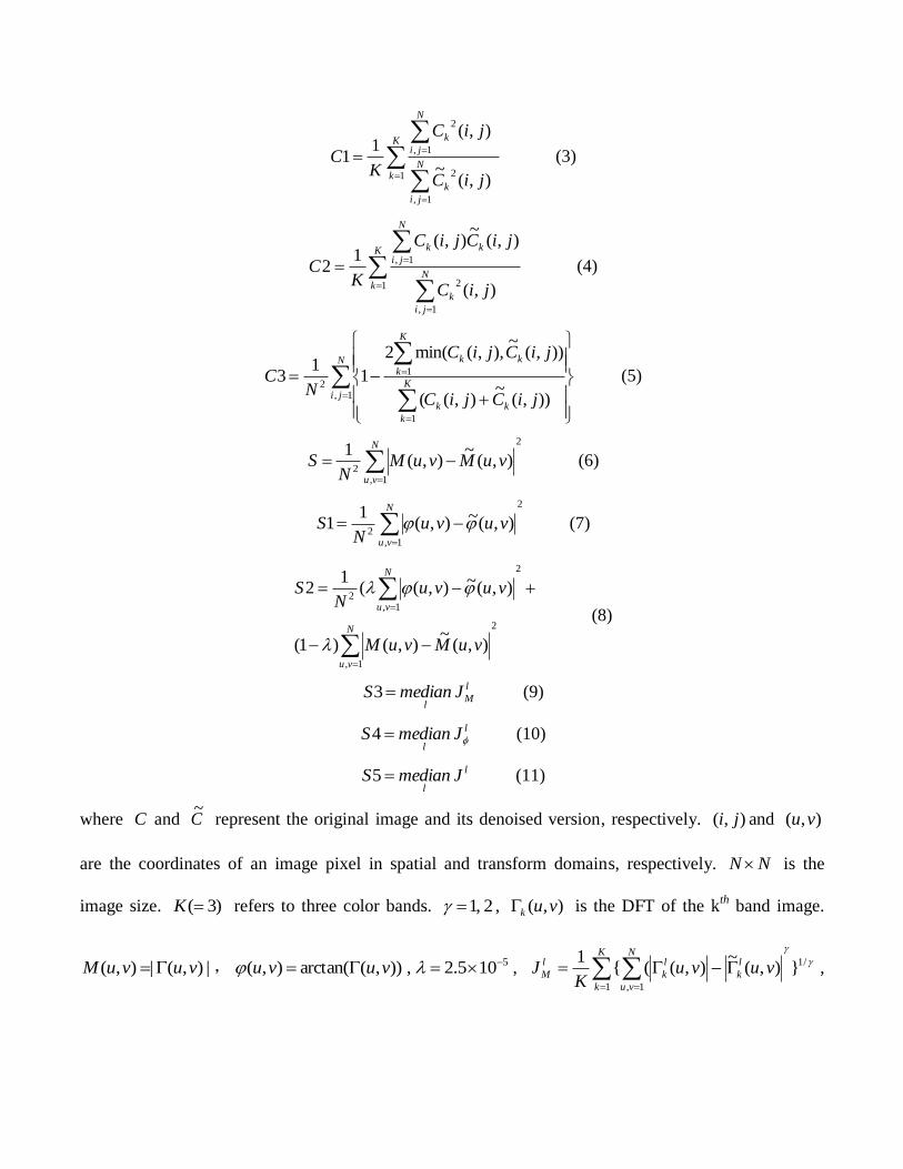
Feature Set III consists of 3+3+6=12 IQMs including three pixel difference-based features, i.e.,

Minkowski difference (1), mean absolute error (2) with 1 , and mean square error (2) with 2 ;

three correlation-based features, i.e., structural content (3), normalized cross correlation (4), and

Czekonowski correlation (5); six spectral features, i.e., spectral magnitude error (6), spectral phase error

(7), spectral phase-magnitude error (8), block spectral magnitude error (9), block spectral phase error

(10), and block spectral phase-magnitude error (11) .

K

k

kk

ji

jiCjiCK1,

),(~

),(1

max (1)

/1

1,2

1

}),(~

),(1

{1

1

N

ji

kk

K

k

jiCjiCNK

M (2)

K

kN

ji

k

N

ji

k

jiC

jiC

KC

1

1,

2

1,

2

),(~

),(1

1 (3)

K

kN

ji

k

N

ji

kk

jiC

jiCjiC

KC

1

1,

2

1,

),(

),(~

),(1

2 (4)

N

jikk

K

k

kk

K

k

jiCjiC

jiCjiC

NC

1,

1

1

2

)),(~

),((

)),(~

),,(min(2

11

3 (5)

2

1,2

),(~

),(1

N

vu

vuMvuMN

S (6)

2

1,2

),(~),(1

1

N

vu

vuvuN

S (7)

2

1,

2

1,2

),(~

),()1(

),(~),((1

2

N

vu

N

vu

vuMvuM

vuvuN

S

(8)

l

Ml

JmedianS 3 (9)

l

lJmedianS 4 (10)

l

lJmedianS 5 (11)

where C and C~

represent the original image and its denoised version, respectively. ),( ji and ),( vu

are the coordinates of an image pixel in spatial and transform domains, respectively. NN is the

image size. )3(K refers to three color bands. 2 ,1 , ),( vuk is the DFT of the kth

band image.

|),(|),( vuvuM ， )),(arctan(),( vuvu , 5105.2 ,

/1

1,1

}),(~

),(({1

N

vu

l

k

l

k

K

k

l

M vuvuK

J ,

/1

1,1

}),(~

),(({1

b

vu

l

k

l

k

K

k

l vuvuK

J , ll

M

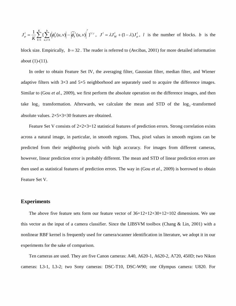
l JJJ )1( , l is the number of blocks. b is the

block size. Empirically, 32b . The reader is referred to (Avcibas, 2001) for more detailed information

about (1)-(11).

In order to obtain Feature Set IV, the averaging filter, Gaussian filter, median filter, and Wiener

adaptive filters with 3×3 and 5×5 neighborhood are separately used to acquire the difference images.

Similar to (Gou et al., 2009), we first perform the absolute operation on the difference images, and then

take 2log transformation. Afterwards, we calculate the mean and STD of the 2log -transformed

absolute values. 2×5×3=30 features are obtained.

Feature Set V consists of 2×2×3=12 statistical features of prediction errors. Strong correlation exists

across a natural image, in particular, in smooth regions. Thus, pixel values in smooth regions can be

predicted from their neighboring pixels with high accuracy. For images from different cameras,

however, linear prediction error is probably different. The mean and STD of linear prediction errors are

then used as statistical features of prediction errors. The way in (Gou et al., 2009) is borrowed to obtain

Feature Set V.

Experiments

The above five feature sets form our feature vector of 36+12+12+30+12=102 dimensions. We use

this vector as the input of a camera classifier. Since the LIBSVM toolbox (Chang & Lin, 2001) with a

nonlinear RBF kernel is frequently used for camera/scanner identification in literature, we adopt it in our

experiments for the sake of comparison.

Ten cameras are used. They are five Canon cameras: A40, A620-1, A620-2, A720, 450D; two Nikon

cameras: L3-1, L3-2; two Sony cameras: DSC-T10, DSC-W90; one Olympus camera: U820. For

simplicity, we index the above ten cameras as X1, X2, X3, X4, X5, X6, X7, X8, X9, and X10,

respectively. To evaluate the capability of these image features in identifying specific cameras, we use

two Canon A620 cameras, i.e., A620-1 and A620-2, and two Nikon L3 cameras, i.e., L3-1 and L3-2. The

photos taken by Canon A620-2 (i.e., X3) and Nikon L3-2 (i.e., X7) are downloaded from

http://www.flickr.com/. Each camera takes 300 photos of natural scenes including buildings, trees, blue

sky and clouds, streets and people. All the photos are saved in JPEG format at the highest resolution each

camera can support. For a fair comparison, we take a 1024×1024 test image block from each photo.

Based on our previous analysis (Li, 2010), each test image is cropped from the center of a photo to avoid

saturated image regions. This selection strategy makes the test image better reflect the original image

content. For each camera, we randomly choose 150 images to form the training set; the rest 150 images

form the test set. Experimental results are shown in the form of confusion matrix, where the first column

and the first row are the test camera index and the predicted camera index, respectively. For clarity of

comparison, the classification rate below 3% is simply denoted as﹡.

From Table 1, our classifier achieves the average accuracy of at least 95% for all cameras except X3

and X7. This result proves that our feature vector is very effective. As for X3 and X7, the correct rates are

88% and 62%, respectively. We owe the decline in accuracy to different image content. The photos taken

by X3 and X7 are downloaded from the internet. It cannot be confirmed whether the photos have been

altered. The only thing we can observe is that the former image set consists of artificial products with

various textile patterns and the image content is usually bright while the latter image set mainly consists

of indoors scenes and the image content is usually dark. In contrast, our photos are mainly natural scenes

with middle intensity. Our detection results coincide with the observation that identification rate is

affected by image content (Tsai &Wang, 2008; Li, 2010).

Using Tables 2-6, we further investigate the performance of each individual feature set. According

to Table 2, the wavelet features have almost the same identification power as the five feature sets all put

together. From Table 5, the statistical features of difference images also have good performance. Such

results are reasonable because these two feature sets are based on the high-frequency component of an

image. On the other hand, the IQMs and statistical features of prediction errors only have moderate

performance according to the results in Tables 4 and 6. In particular, the color features only lead to the

accuracy of 47%, as shown in Table 3. It seems that this feature set contributes the least to our sample

classifier.

ROBUSTNESS OF OUR SAMPLE CLASSIFIER

For real-world applications, camera identifiers should have the capability in tackling images that have

undergone different image manipulations. Some manipulations are probably not malicious attacks but

normal ways for saving storage space or emphasizing part of image content. We evaluate the robustness

of our classifier under three common image manipulations: JPEG compression, cropping, and scaling.

Note that each test image has undergone only one type of manipulation for each case. We do not consider

the combined effect of different manipulations to avoid making the analysis too complex.

Experimental Results under Compression

We take JPEG compression with quality factor 70. From Table 7, the average accuracy is 43%.

Compared with Table 1, the performance of the classifier greatly decreases. We further investigate the

performance of each individual feature set. From Feature Sets I to V, the correct identification rates are

21%, 46%, 31%, 24%, and 33%, respectively. Apparently, the performance of each feature set degrades.

Among them, Feature Set I has the sharpest decline in performance (see Table 8). The possible reason is

that compression makes more high-frequency coefficients equal zero. On the other side, the performance

of Feature Set II is a little surprising. The classifier has the average accuracy of 46%. Compared with the

accuracy before compression (47%), there is only a slight decline. This implies that compression has

little impact on Feature Set II (color features).

Experimental Results under Cropping

We remove 1/8 image region from the original image to simulate a cropping manipulation.

According to Table 9, the average accuracy is 39%. From Feature Sets I to V, the correct identification

rates are 35%, 32%, 25%, 84%, and 25%, respectively. It can be seen that Feature Sets III and V are

more sensitive to cropping. The possible reason is that the pixels in the removed image regions are

replaced with value 0 and such replacement affects the measurement of IQMs (see Table 10).

Meanwhile, the removed and replaced regions can be thought of as smooth regions. Their appearance

probably affects the performance of statistical features of prediction errors (see Table 11). In contrast,

Feature Set IV maintains good performance. Thus, cropping does not affect Feature Set IV (statistical

features of difference images) too much.

Experimental Results under Scaling

We shrink the test images with scaling factor 0.9. According to Table 12, the accuracy is 53%. From

Feature Sets I to V, the correct identification rates are 32%, 47%, 39%, 58%, and 49%, respectively.

Feature Set I has the greatest decline in performance (see Table 13). The possible reason is that wavelet

features are fragile to geometrical distortions such as scaling. On the other side, Feature Set IV

(statistical features of difference images) still has the best performance. In other words, Feature Set IV is

not very sensitive to small scaling operations.

PERFORMANCE OF CLASSIFIER ON A LARGER CAMERA DATABASE

To investigate the impact of large camera databases on the performance of our sample classifier, nine

more cameras have been added for this experiment. We list all of nineteen cameras in Table 14. For a

fair comparison, all the experiment requirements and environments keep the same as those used for 10

cameras.

From Table 15, the classifier achieves the average accuracy of 86% for nineteen cameras. Compared

to the accuracy of 92% for ten cameras, its accuracy decreases by 6 percentage points. Therefore, the

overall performance of this classifier may drop with larger database size.

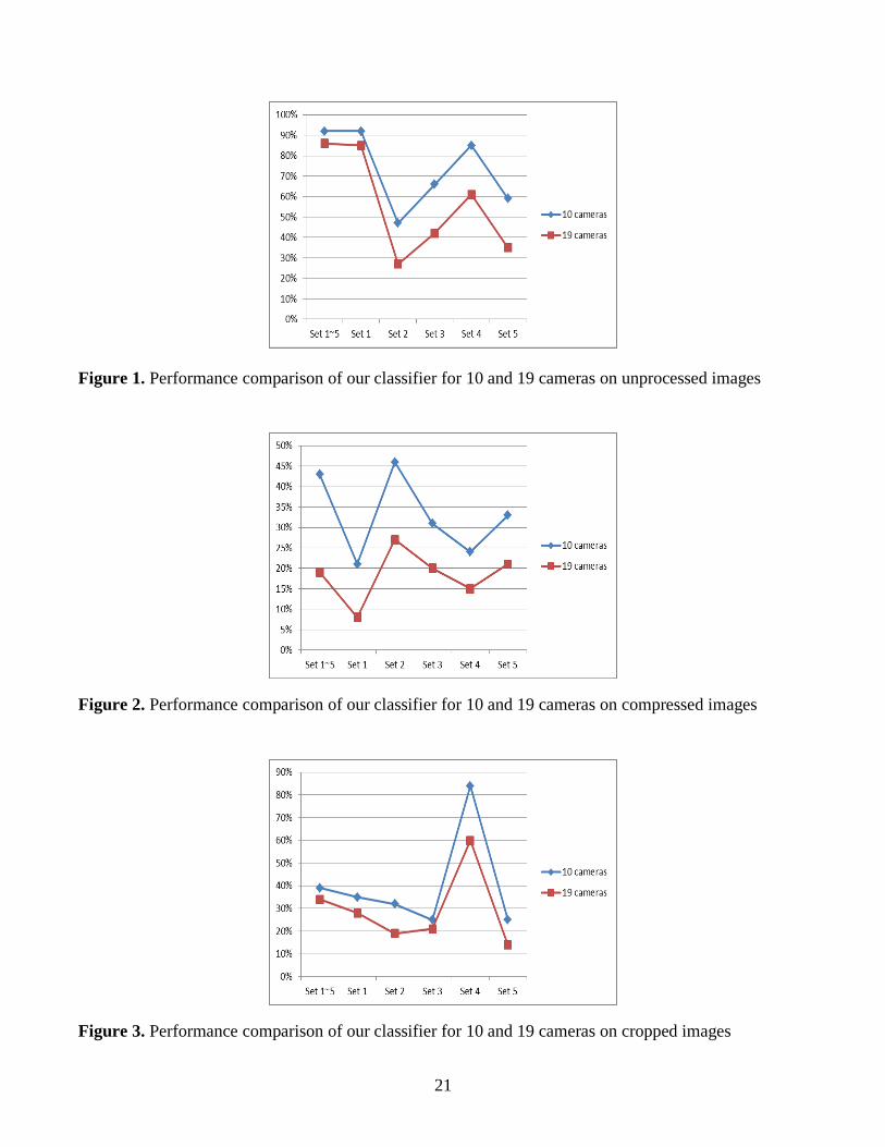
In order to analyze the performance of each feature set, we use one feature set a time. The accuracy

of our classifier using the wavelet feature set is 85%, which is very close to the accuracy of using all the

feature sets. Compared with Table 2, it decreases by 7 percentage points. So the degree of decrease is

very similar to what we have for 10 cameras under the conditions of using all the feature sets and of using

the wavelet feature set alone. According to Figure 1, Feature Set II, III, IV, and V decrease 20 to 24

percentage points in performance.

Experimental Results under Compression

As shown in Figure 2, the average accuracy of our sample classifier for nineteen cameras is 19% and

it decreases by 24 percentage points compared to that for ten cameras. The individual accuracy for

Feature Sets I to V are 8%, 27%, 20%, 15%, and 21%, respectively. Compared with the situation for ten

cameras, the decrease tendency of performance is same. However, compared with Figures 2, 3, and 4, it

can be found that compression has the greatest impact on the performance of our classifier. The robust

feature set against compression is still Feature Set II, i.e., color features.

Experimental Results under Cropping

According to Figure 3, the average accuracy of our sample classifier for nineteen cameras is 34%.

There are 5 percentage points lower than that for ten cameras. The individual accuracies for Feature Sets I

to V are 28%, 19%, 21%, 60%, and 14% in sequence, and are 7, 13, 4, 24, and 11 percentage points

lower than their counterparts for ten cameras, respectively. Still Feature Set IV has the best performance.

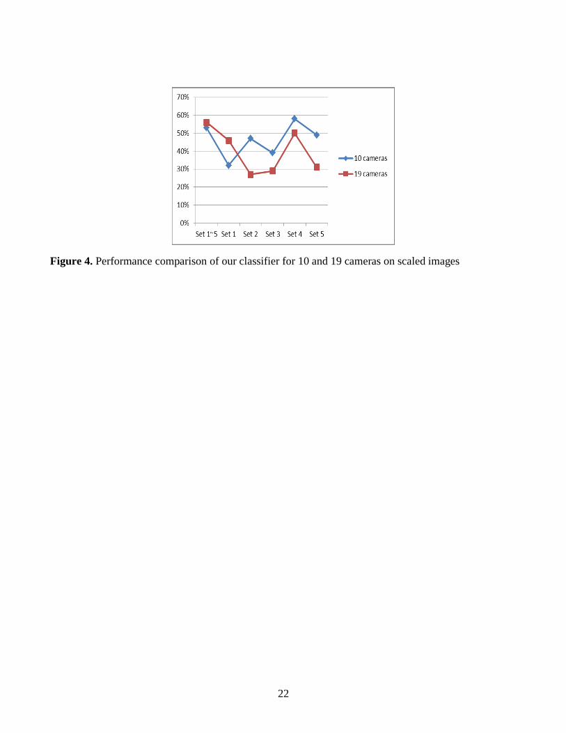
Experimental Results under Scaling

According to Figure 4, the average accuracy of our sample classifier is 56% which is 3 percentage

points higher than the accuracy of our sample classifier for ten cameras. The individual accuracies for

Feature Sets I to V are 46%, 27%, 29%, 50%, and 31%, respectively. Compared with the situation for ten

cameras, we can find the performance of the Feature Set II becomes worse quickly; on the other hand,

both the performance of our sample classifier using all the feature sets and that of using Feature Set I

become better than their counterparts for ten cameras. These phenomena are a little strange. So far we

have not found suitable explanations.

CONCLUSIONS

The issue of selecting image features for robust camera identification has not been thoroughly addressed

in literature. In this paper, we have discussed the performance as well as the robustness of a sample

classifier. We first use a small camera database to investigate the overall performance of the classifier and

the individual performance of each feature set, and then, we repeat our test on a larger camera database.

Experiments have shown that the accuracy has a trend of decrease when the database becomes larger.

However, some phenomena still need further investigation such as those happened in Section IV.C.

The problem of camera identification is a complex one with no universally applicable solution. Our

efforts in this work only reveal the deficiency of a camera classifier which has been designed without

considering the robustness against common image processing. It is inferred from our experiments that the

use of many different types of image features can benefit the robustness of camera classifiers. Moreover,

even when decreasing the number of features for the sake of computational efficiency, the selection of

reduced feature set has to take the robustness into account. The selection of suitable feature set is our

future work.

ACKNOWLEDGEMENT

This work is partially supported by the NSF of China (Project No. 60772115) and the EU FP7 Digital

Image and Video Forensics project (Grant Agreement No. 251677).

REFERENCES

Avcibas. I. (2001). Image quality statistics and their use in steganalysis and compression. Ph.D. Thesis,

Bogazici University.

Avcibas, I., Memon, N., & Sankur, B. (2003). Steganalysis using image quality metrics. IEEE

Transactions on Image Processing, 12(2), 221-229.

Chang, C.-C., & Lin, C.-J. (2001). LIBSVM: A Library for Support Vector Machines.

http://www.csie.ntu.edu.tw/~cjlin/

Farid, H., & Lyu, S. (2002). Detecting hidden messages using higher-order statistics and support vector

machines. Proceedings of 5th International Workshop on Information Hiding, Springer-Verlag,

Berlin, Heidelberg, 2578, 340-354.

Filler, T., Fridrich, J., & Goljan, M. (2008). Using sensor pattern noise for camera model identification.

Proceedings of IEEE International Conference on Image Processing, 1296-1299.

Gloe, T., Kirchner, M., Winkler, P., & Bohme, R. (2007). Can we trust digital image forensics.

Proceedings of the 15th International Conference on Multimedia, 78-86.

Gou, H., Swaminathan, A., & Wu, M. (2009). Intrinsic sensor noise features for forensic analysis on

scanners and scanned images. IEEE Transactions on Information Forensics Security, 4(3), 476-491.

Khanna, N., Mikkilineni, A.K., & Delp, E.J. (2009). Scanner identification using feature-based

processing and analysis. IEEE Transactions on Information Forensics Security, 4(1), 123-139.

Kharrazi, M., Sencar, H.T., & Memon, N. (2004). Blind source camera identification. Proceedings of

IEEE International Conference on Image Processing, Singapore, 709-712.

Li, C.-T. (2010). Source camera identification using enhanced sensor pattern noise. IEEE Transactions

on Information Forensics Security, 5(2), 280-287.

Lukas, J., Fridrich, J., & Goljan, M. (2006). Digital camera identification from sensor pattern noise.

IEEE Transactions on Information Forensics Security, 1(2), 205-214.

Tsai, M.-J., Lai, C.-L., & Liu, J. (2007). Camera/Mobile phone source identification for digital forensics.

Proceedings of IEEE International Conference on Acoustics, Speech and Signal Processing,

221-224.

Tsai M.-J., & Wang, C.-S. (2008). Adaptive feature selection for digital camera source identification.

Proceedings of IEEE International Symposium on Ciruits and Systems, 412-415.

Tsai, M.-J., & Wu, G.-H. (2006). Using image features to identify camera sources. Proceedings of IEEE

International Conference on Acoustics, Speech and Signal Processing, 2,297-300.

Table 1. Confusion matrix for our sample classifier using all the five feature sets. Accuracy = 92% (1383/1500)

X1 X2 X3 X4 X5 X6 X7 X8 X9 X10

X1 97 * * * * * * * * *

X2 3 95 * * * * * * * *

X3 * * 88 6 * * * * * *

X4 * * * 96 * * * * * *

X5 * * * * 98 * * * * *

X6 * * * * * 98 * * * *

X7 * * * * 21 8 61 * * 5

X8 * * * * * * * 99 * *

X9 * * * * * * * * 95 *

X10 * * * * * * * * * 95

Table 2. Confusion matrix for our sample classifier using only Feature Set I. Accuracy = 92%

(1382/1500)

X1 X2 X3 X4 X5 X6 X7 X8 X9 X10

X1 95 * * * * * * * * *

X2 * 97 * * * * * * * *

X3 * * 83 7 * * 7 * * *

X4 * * * 91 * 6 * * * *

X5 * * * * 94 * * * * *

X6 * * * * * 95 * * * *

X7 * * * * 5 3 87 * * *

X8 * 3 * * * * * 97 * *

X9 5 * * * * * * * 91 *

X10 * * * * * * 6 * * 93

Table 3. Confusion matrix for our sample classifier using only Feature Set II. Accuracy = 47%

(702/1500)

X1 X2 X3 X4 X5 X6 X7 X8 X9 X10

X1 64 * * * 6 8 * * 9 7

X2 2* 4* * * 13 9 * 3 8 5

X3 * * 81 3 * 7 * * * 3

X4 7 17 * 45 4 9 * 5 * 9

X5 4 7 * 5 38 17 * 3 12 9

X6 15 6 * 12 11 43 * 3 6 *

X7 6 9 13 7 7 * 43 * 9 4

X8 3 11 * 7 24 15 * 29 * 5

X9 9 1* 7 9 13 13 * 3 35 *

X10 * 5 * 9 4 12 * 10 5 51

Table 4. Confusion matrix for our sample classifier using only Feature Set III. Accuracy = 66%

(987/1500)

X1 X2 X3 X4 X5 X6 X7 X8 X9 X10

X1 77 7 * 11 * * * * * *

X2 2* 61 * 9 * * * * * *

X3 * * 81 11 * * * * * *

X4 11 13 6 58 * 5 * * * *

X5 5 * * * 88 * 5 * * *

X6 4 5 * * 4 7* * 4 1* *

X7 * 7 * 7 12 * 52 5 4 7

X8 * 4 4 5 5 * 17 56 3 *

X9 * 4 * * 6 11 17 13 45 *

X10 * * * 4 3 * 11 9 * 69

Table 5. Confusion matrix for our sample classifier using only Feature Set IV. Accuracy = 85%

(1277/1500)

X1 X2 X3 X4 X5 X6 X7 X8 X9 X10

X1 83 1* * * * * * * * *

X2 12 85 * * * 3 * * * *

X3 * * 87 7 * * * * * *

X4 * * * 87 * * * * 5 *

X5 * * * * 99 * * * * *

X6 5 * * * * 83 4 * 3 *

X7 * * * * 10 * 73 * 7 3

X8 * * * * * * * 95 * *

X9 5 * * * * * 4 8 75 *

X10 4 * * * 5 * 3 * * 85

Table 6. Confusion matrix for our sample classifier using only Feature Set V. Accuracy = 59%

(898/1500)

X1 X2 X3 X4 X5 X6 X7 X8 X9 X10

X1 83 3 * * * 5 * * * *

X2 10 43 * 5 5 23 * * 6 3

X3 * 5 73 7 * * * 5 * 4

X4 * 4 7 67 * 7 * 5 * 3

X5 * * * * 85 * * 5 * 5

X6 * 21 4 5 * 53 * * 10 *

X7 3 5 3 5 9 * 45 8 12 7

X8 * * * * 26 * * 59 * 4

X9 * 7 5 5 11 9 * 10 40 8

X10 5 * * 5 16 4 * 11 * 52

Table 7. Confusion matrix for our sample classifier using all the five feature sets. Accuracy = 43%

(638/1500)

X1 X2 X3 X4 X5 X6 X7 X8 X9 X10

X1 57 * 5 4 3 15 11 * * 4

X2 31 21 * 4 4 18 15 * * 5

X3 17 * 39 * 3 12 21 * * 5

X4 7 * * 21 5 7 44 * * 15

X5 * * 4 * 73 * 23 * * *

X6 4 * * * 5 65 21 * * *

X7 7 * * * 8 5 73 * * 4

X8 4 3 6 * 19 * 65 * * *

X9 13 * * * 21 22 35 * * *

X10 * * * * 8 * 11 * * 75

Table 8. Confusion matrix for our sample classifier using only Feature Set I. Accuracy = 21%

(319/1500)

X1 X2 X3 X4 X5 X6 X7 X8 X9 X10

X1 12 3 * * * * 79 * * 4

X2 * 19 * * * * 73 * * 4

X3 * * 23 * * 10 58 * * 6

X4 * * * 12 * * 74 * * 10

X5 * * * * 4 * 96 * * *

X6 * * * * * * 93 * * *

X7 * * * * 4 4 87 * * *

X8 4 8 * * * * 86 * * *

X9 6 * * * 12 13 65 * * *

X10 * * * * * * 46 * * 53

Table 9. Confusion matrix for our sample classifier using all the five feature sets. Accuracy = 39%

(581/1500)

X1 X2 X3 X4 X5 X6 X7 X8 X9 X10

X1 63 5 7 * * * * * * 24

X2 5 57 9 4 * * * * * 23

X3 * * 37 57 * * * * * 5

X4 * * 7 74 * * * * * 15

X5 * * 84 * * * * * * 13

X6 * * 7 13 * 45 * * * 31

X7 * * 65 4 * * 4 * * 24

X8 * 11 45 13 * * * 6 * 23

X9 3 * 16 5 4 * * * 33 37

X10 * * 30 * * * * * * 66

Table 10. Confusion matrix for our sample classifier using only Feature Set III. Accuracy = 25%

(380/1500)

X1 X2 X3 X4 X5 X6 X7 X8 X9 X10

X1 49 * 6 23 * 4 3 * 11 *

X2 46 * 7 19 4 11 * * 9 *

X3 40 * 31 17 * 4 * * * *

X4 31 * * 24 5 9 * * 20 *

X5 * * 8 6 51 * 23 * * 7

X6 17 * 4 18 10 21 * * 26 *

X7 3 * 9 21 18 9 25 * * 9

X8 5 * 5 17 11 17 19 * 19 3

X9 11 * * 20 25 7 9 * 17 7

X10 9 * 5 14 8 3 13 * 13 31

Table 11. Confusion matrix for our sample scheme using Feature Set V. Accuracy = 25% (371/1500)

X1 X2 X3 X4 X5 X6 X7 X8 X9 X10

X1 90 * * * * * 4 * * *

X2 87 * * * * * 6 * * *

X3 71 9 11 * * 3 * * * *

X4 61 13 * 5 * 10 5 * * 4

X5 23 * * * 59 * 10 * 4 *

X6 87 * * * * 7 * * * *

X7 27 * * * 5 * 50 * 11 *

X8 41 6 * * 28 * 17 * * 3

X9 62 6 * * * 7 11 * 3 9

X10 39 * * * 8 13 12 * 5 21

Table 12. Confusion matrix for our sample classifier using all the five feature sets. Accuracy = 53%

(793/1500)

X1 X2 X3 X4 X5 X6 X7 X8 X9 X10

X1 48 * * * * 45 * * * *

X2 24 30 * * 7 38 * * * *

X3 * 8 71 9 * * * * * 4

X4 * 20 * 37 11 15 6 * * 8

X5 3 * * * 96 * * * * *

X6 * * * * 5 89 * * * *

X7 * * * * 20 6 64 * * 4

X8 5 55 * * 30 * 7 * * *

X9 6 17 * * 24 30 19 * * *

X10 * * * * 3 * 3 * * 91

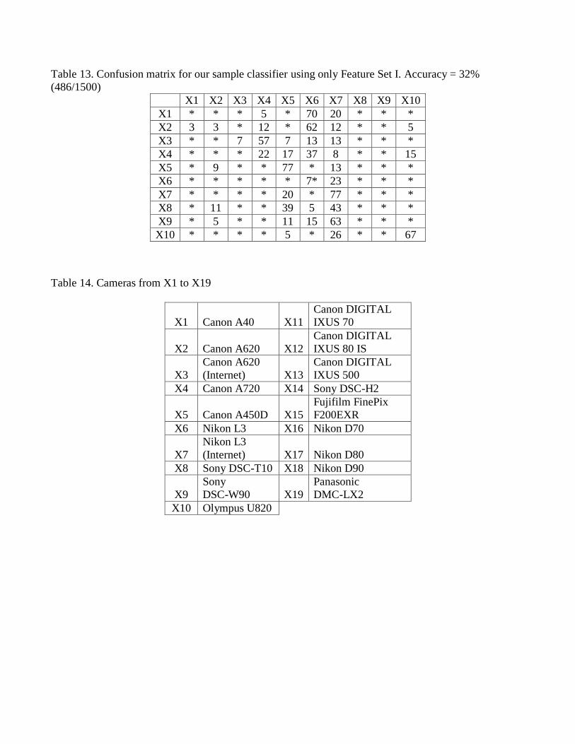
Table 13. Confusion matrix for our sample classifier using only Feature Set I. Accuracy = 32%

(486/1500)

X1 X2 X3 X4 X5 X6 X7 X8 X9 X10

X1 * * * 5 * 70 20 * * *

X2 3 3 * 12 * 62 12 * * 5

X3 * * 7 57 7 13 13 * * *

X4 * * * 22 17 37 8 * * 15

X5 * 9 * * 77 * 13 * * *

X6 * * * * * 7* 23 * * *

X7 * * * * 20 * 77 * * *

X8 * 11 * * 39 5 43 * * *

X9 * 5 * * 11 15 63 * * *

X10 * * * * 5 * 26 * * 67

Table 14. Cameras from X1 to X19

X1 Canon A40 X11

Canon DIGITAL

IXUS 70

X2 Canon A620 X12

Canon DIGITAL

IXUS 80 IS

X3

Canon A620

(Internet) X13

Canon DIGITAL

IXUS 500

X4 Canon A720 X14 Sony DSC-H2

X5 Canon A450D X15

Fujifilm FinePix

F200EXR

X6 Nikon L3 X16 Nikon D70

X7

Nikon L3

(Internet) X17 Nikon D80

X8 Sony DSC-T10 X18 Nikon D90

X9

Sony

DSC-W90 X19

Panasonic

DMC-LX2

X10 Olympus U820

Table 15. Confusion matrix for our sample classifier using all feature sets on unprocessed images.

Accuracy = 86% (2451/2850) (classification)

X1 X2 X3 X4 X5 X6 X7 X8 X9 X10 X11 X12 X13 X14 X15 X16 X17 X18 X19

X1 97 * * * * * * * * * * * * * * * * * *

X2 3 94 * * * * * * * * * * * * * * * * *

X3 * * 86 7 * * * * * * * * * * * * * * *

X4 * * * 95 * 3 * * * * * * * * * * * * *

X5 * * * * 97 * * * * * * * * * * * * * *

X6 * * * * * 97 * * * * * * * * * * * * *

X7 * * 3 * 14 * 57 * * * * * * * 5 * 6 * 5

X8 * * * * * * * 99 * * * * * * * * * * *

X9 * * * * * * * * 91 * * * * * * * * * 4

X10 * * * * * * * * * 91 * * * * * 3 * * *

X11 * * * * * 15 * * * * 81 * * * 1 * * * *

X12 * 10 * * * * 5 * * * * 67 4 * * * * * 5

X13 * 3 * * * 3 * * * * * 7 71 * 3 * 4 3 *

X14 * * * * * * * * * * * * * 94 * * * * *

X15 3 * 3 7 * 5 * * * * * * * * 74 * * * *

X16 * * * 3 * * * * * * * * * * * 88 3 * *

X17 * * * * * * 9 * * * * * 4 * 3 * 79 * *

X18 * 3 * * * * * * * * * * * * * * * 92 *

X19 * * * * * * * * 5 * * * * * * * * * 84

21

Figure 1. Performance comparison of our classifier for 10 and 19 cameras on unprocessed images

Figure 2. Performance comparison of our classifier for 10 and 19 cameras on compressed images

Figure 3. Performance comparison of our classifier for 10 and 19 cameras on cropped images

22

Figure 4. Performance comparison of our classifier for 10 and 19 cameras on scaled images