sounding the troposphere by leo-leo occultation: …wegc...16-20 september 2002 opac-1, graz,...
TRANSCRIPT
16-20 September 2002 OPAC-1, Graz, Austria 1
Sounding the Troposphere by LEO-LEO Occultation: A Simulation Retrieval System
and Performance Analysis Results
Stephen Leroy1, Chi O. AoJet Propulsion Laboratory
California Institute of Technology
1Done in part while visiting the Danish Meteorological Institute
16-20 September 2002 OPAC-1, Graz, Austria 2
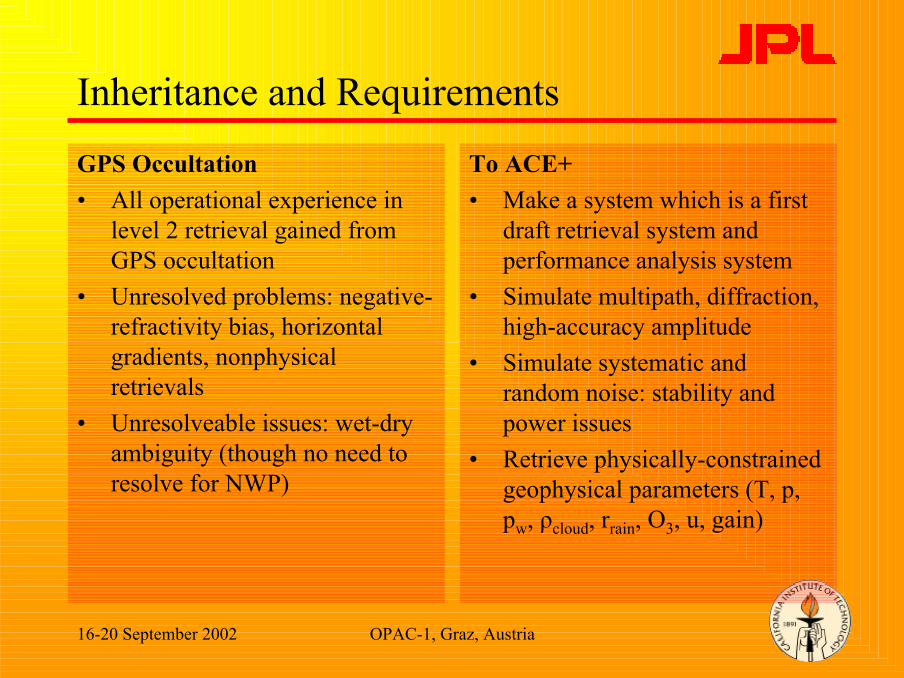
Inheritance and Requirements
GPS Occultation • All operational experience in
level 2 retrieval gained from GPS occultation
• Unresolved problems: negative-refractivity bias, horizontal gradients, nonphysical retrievals
• Unresolveable issues: wet-dry ambiguity (though no need to resolve for NWP)
To ACE+• Make a system which is a first
draft retrieval system and performance analysis system
• Simulate multipath, diffraction, high-accuracy amplitude
• Simulate systematic and random noise: stability and power issues
• Retrieve physically-constrained geophysical parameters (T, p, pw, ρcloud, rrain, O3, u, gain)
16-20 September 2002 OPAC-1, Graz, Austria 3
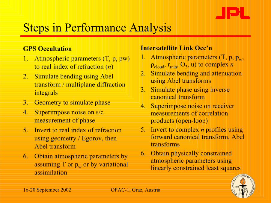
Steps in Performance AnalysisGPS Occultation1. Atmospheric parameters (T, p, pw)
to real index of refraction (n)2. Simulate bending using Abel
transform / multiplane diffraction integrals
3. Geometry to simulate phase4. Superimpose noise on s/c
measurement of phase5. Invert to real index of refraction
using geometry / Egorov, then Abel transform
6. Obtain atmospheric parameters by assuming T or pw or by variational assimilation
Intersatellite Link Occ’n 1. Atmospheric parameters (T, p, pw,
ρcloud, rrain, O3, u) to complex n2. Simulate bending and attenuation
using Abel transforms3. Simulate phase using inverse
canonical transform4. Superimpose noise on receiver
measurements of correlation products (open-loop)
5. Invert to complex n profiles using forward canonical transform, Abel transforms
6. Obtain physically constrained atmospheric parameters using linearly constrained least squares
16-20 September 2002 OPAC-1, Graz, Austria 4
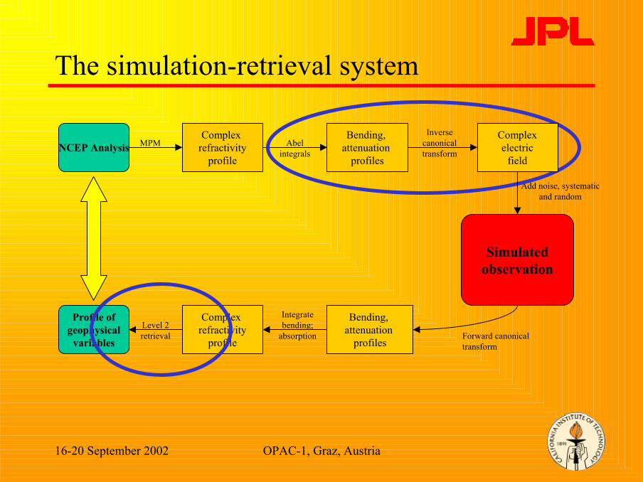
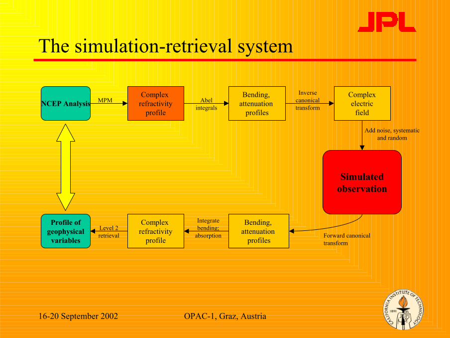
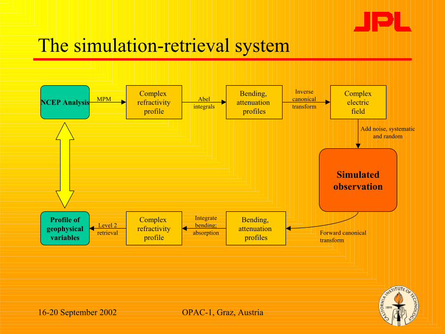
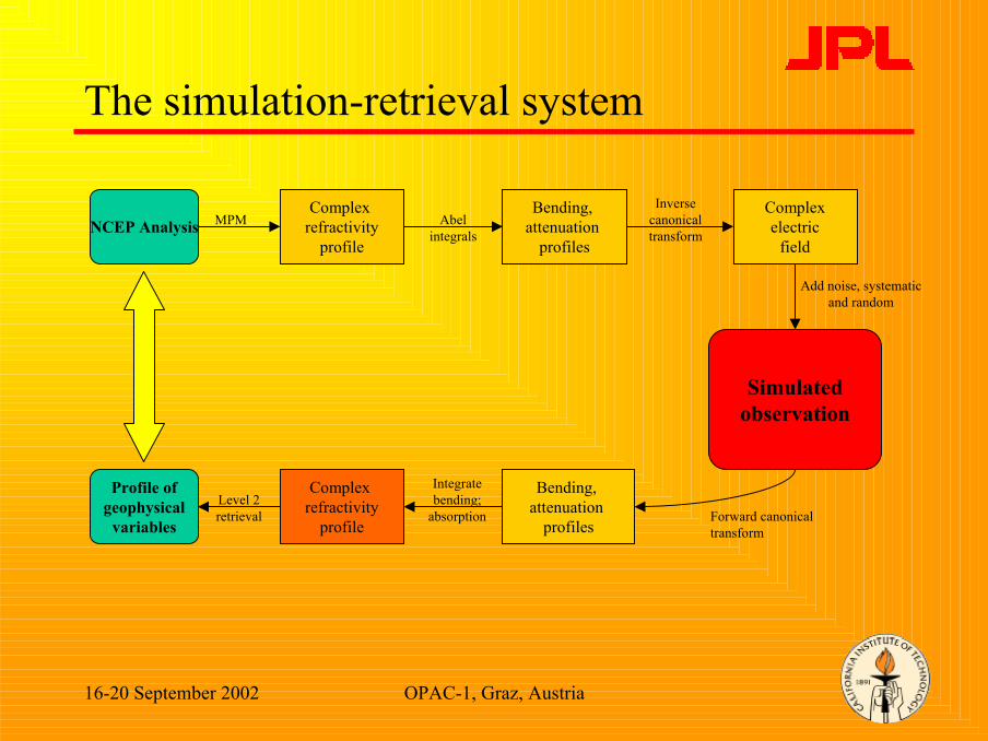
The simulation-retrieval system
NCEP AnalysisComplex
refractivityprofile
Simulatedobservation
Bending, attenuation
profiles
Complex refractivity
profile
Profile ofgeophysical
variables
MPMInverse
canonical transform
Add noise, systematicand random
Integrate bending;
absorptionLevel 2 retrieval
Bending, attenuation
profiles
Abel integrals
Forward canonical transform
Complexelectric
field
16-20 September 2002 OPAC-1, Graz, Austria 5
The simulation-retrieval system
NCEP AnalysisComplex
refractivityprofile
Simulatedobservation
Bending, attenuation
profiles
Complex refractivity
profile
Profile ofgeophysical
variables
MPMInverse
canonical transform
Add noise, systematicand random
Integrate bending;
absorptionLevel 2 retrieval
Bending, attenuation
profiles
Abel integrals
Forward canonical transform
Complexelectric
field
16-20 September 2002 OPAC-1, Graz, Austria 6
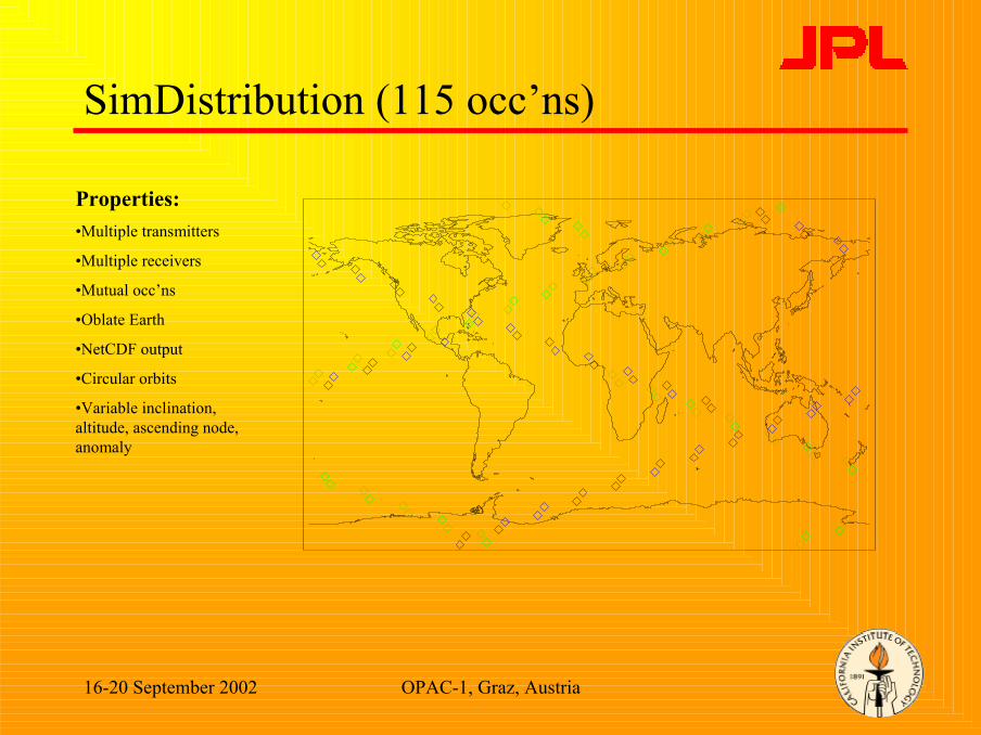
SimDistribution (115 occ’ns)
Properties:•Multiple transmitters
•Multiple receivers
•Mutual occ’ns
•Oblate Earth
•NetCDF output
•Circular orbits
•Variable inclination, altitude, ascending node, anomaly
16-20 September 2002 OPAC-1, Graz, Austria 7
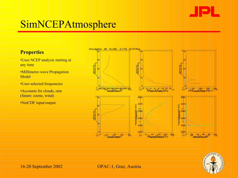
SimNCEPAtmosphere
0.00 0.05 0.10 0.15 0.20Attenuation (dB/km)
0
5
10
15
Alti
tude
(km
)
0.00 0.05 0.10 0.15 0.20Attenuation (dB/km)
0
5
10
15
Alti
tude
(km
)
0.00 0.05 0.10 0.15 0.20Attenuation (dB/km)
0
5
10
15
Alti
tude
(km
)
0.00 0.05 0.10 0.15 0.20Attenuation (dB/km)
0
5
10
15
Alti
tude
(km
)
0.00 0.05 0.10 0.15 0.20Attenuation (dB/km)
0
5
10
15
Alti
tude
(km
)0.00 0.05 0.10 0.15 0.20
Attenuation (dB/km)
0
5
10
15
Alti
tude
(km
)
Properties•Uses NCEP analysis starting at any time
•Millimeter-wave Propagation Model
•User-selected frequencies
•Accounts for clouds, rain (future: ozone, wind)
•NetCDF input/output
Occultation 56: 15.34E, -0.11N, 22.914hrs
180 200 220 240 260 280 300 320Temperature (K)
0
10
20
30
40
Alti
tude
(km
)
0 2 4 6 8 10 12 14Specific Humidity (g/kg)
0
10
20
30
40
Alti
tude
(km
)
0 50 100 150 200Cloud Liquid Water (mg/m3)
0
10
20
30
40
Alti
tude
(km
)
0 5 10 15 20Ozone (mg/m3)
0
10
20
30
40A
ltitu
de (
km)
0 50 100 150 200Integrated Bending (m)
6330
6340
6350
6360
6370
6380
Impa
ct P
aram
eter
(km
)0 20 40 60 80 100
Attenuation (dB)
6330
6340
6350
6360
6370
6380
Impa
ct P
aram
eter
(km
)
16-20 September 2002 OPAC-1, Graz, Austria 8
The simulation-retrieval system
NCEP AnalysisComplex
refractivityprofile
Simulatedobservation
Bending, attenuation
profiles
Complex refractivity
profile
Profile ofgeophysical
variables
MPMInverse
canonical transform
Add noise, systematicand random
Integrate bending;
absorptionLevel 2 retrieval
Bending, attenuation
profiles
Abel integrals
Forward canonical transform
Complexelectric
field
16-20 September 2002 OPAC-1, Graz, Austria 9
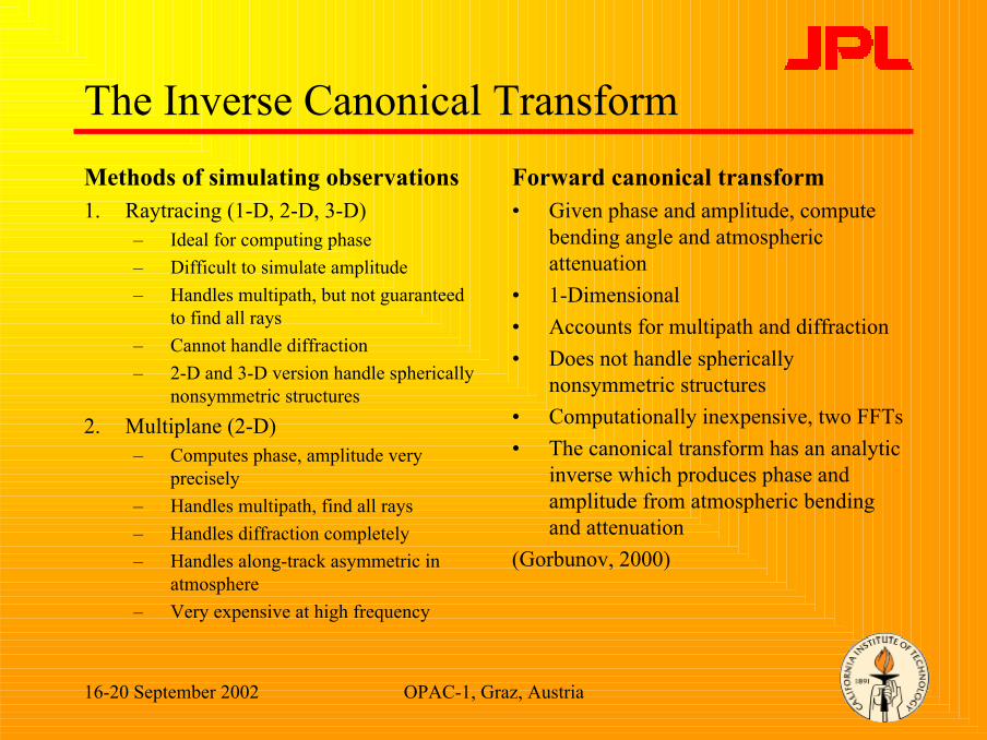
The Inverse Canonical TransformMethods of simulating observations1. Raytracing (1-D, 2-D, 3-D)
– Ideal for computing phase– Difficult to simulate amplitude– Handles multipath, but not guaranteed
to find all rays– Cannot handle diffraction– 2-D and 3-D version handle spherically
nonsymmetric structures2. Multiplane (2-D)
– Computes phase, amplitude very precisely
– Handles multipath, find all rays– Handles diffraction completely– Handles along-track asymmetric in
atmosphere– Very expensive at high frequency
Forward canonical transform• Given phase and amplitude, compute
bending angle and atmospheric attenuation
• 1-Dimensional• Accounts for multipath and diffraction• Does not handle spherically
nonsymmetric structures• Computationally inexpensive, two FFTs• The canonical transform has an analytic
inverse which produces phase and amplitude from atmospheric bending and attenuation
(Gorbunov, 2000)
16-20 September 2002 OPAC-1, Graz, Austria 10
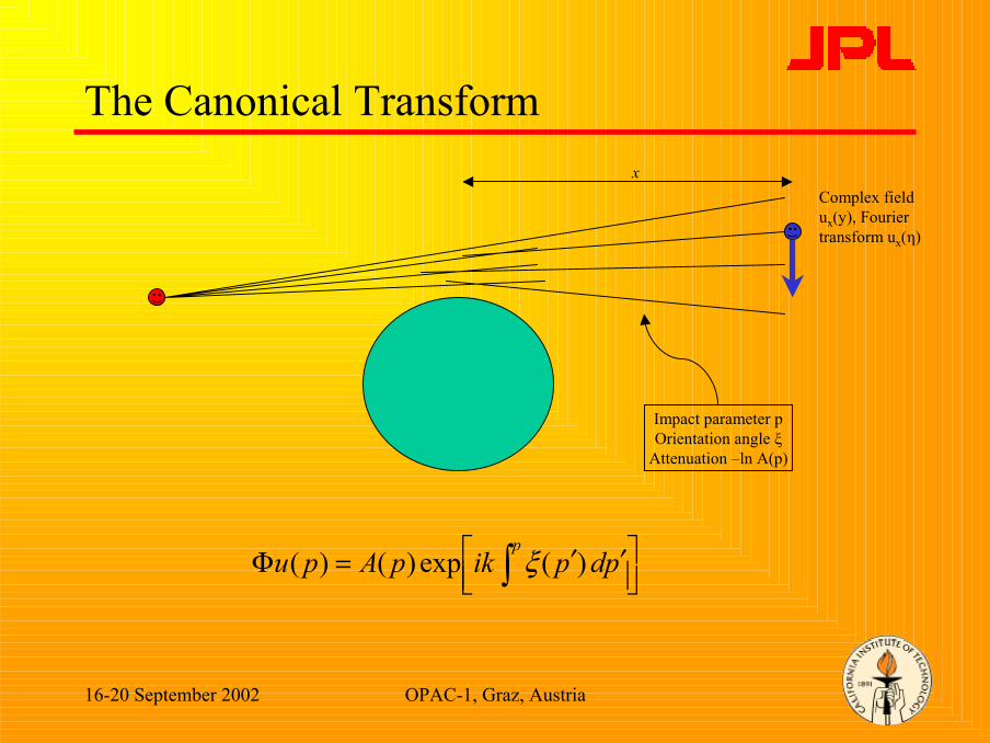
The Canonical Transform
Complex field ux(y), Fourier transform ux(η)
Impact parameter pOrientation angle ξ
Attenuation –ln A(p)
′′=Φ ∫
ppdpikpApu )(exp)()( ξ
x
16-20 September 2002 OPAC-1, Graz, Austria 11
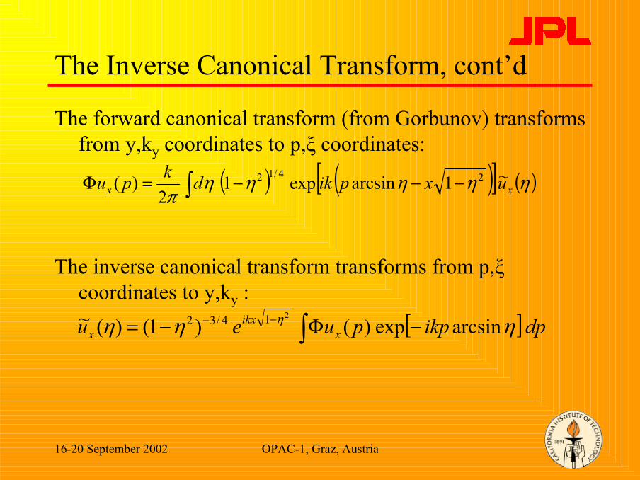
The Inverse Canonical Transform, cont’d
The forward canonical transform (from Gorbunov) transforms from y,ky coordinates to p,ξ coordinates:
The inverse canonical transform transforms from p,ξcoordinates to y,ky :
( ) ( )[ ] ( )ηηηηηπ xx uxpikdkpu ~1arcsinexp1
2)( 24/12 −−−=Φ ∫
[ ]dpikppueu xikx
x ηηη η arcsinexp)()1()(~ 214/32 −Φ−= ∫−−
16-20 September 2002 OPAC-1, Graz, Austria 12
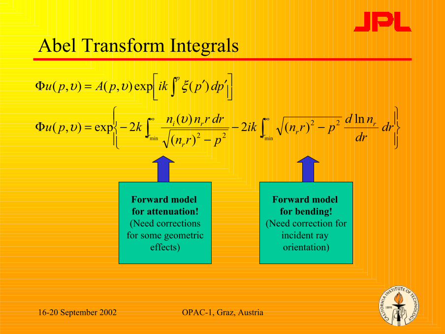
Abel Transform Integrals
′′=Φ ∫
ppdpikpApu )(exp),(),( ξυυ
−−−
−=Φ ∫∫∞∞
minmin
ln)(2)(
)(2exp),( 22
22 rr
rrr
ri drdr
ndprnikprndrrnnkpu υυ
Forward model for attenuation!(Need corrections
for some geometriceffects)
Forward model for bending!
(Need correction forincident ray orientation)
16-20 September 2002 OPAC-1, Graz, Austria 13
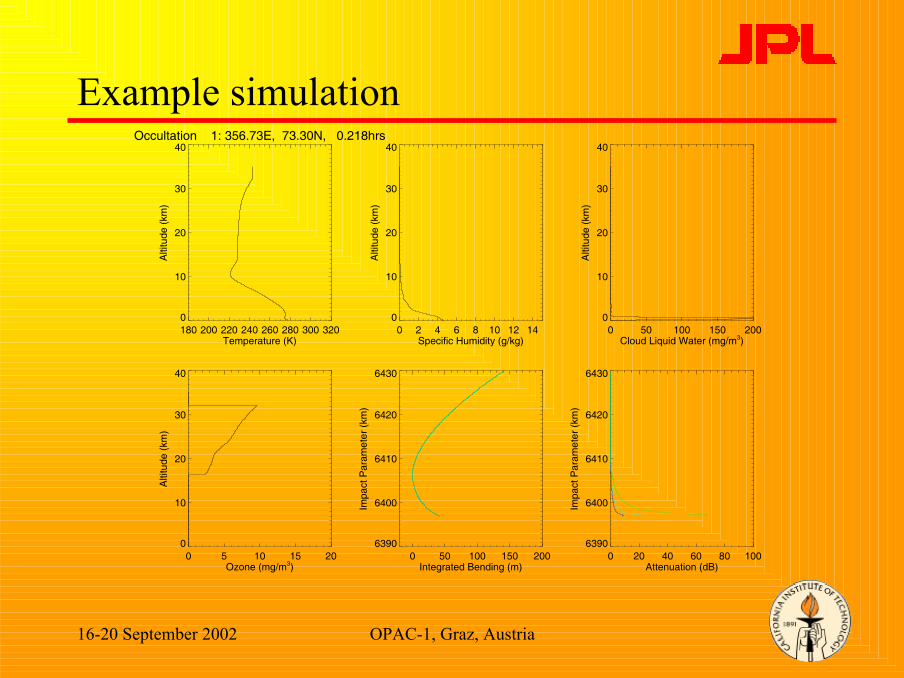
Example simulationOccultation 1: 356.73E, 73.30N, 0.218hrs
180 200 220 240 260 280 300 320Temperature (K)
0
10
20
30
40
Alti
tude
(km
)
0 2 4 6 8 10 12 14Specific Humidity (g/kg)
0
10
20
30
40
Alti
tude
(km
)
0 50 100 150 200Cloud Liquid Water (mg/m3)
0
10
20
30
40
Alti
tude
(km
)
0 5 10 15 20Ozone (mg/m3)
0
10
20
30
40
Alti
tude
(km
)
0 50 100 150 200Integrated Bending (m)
6390
6400
6410
6420
6430Im
pact
Par
amet
er (
km)
0 20 40 60 80 100Attenuation (dB)
6390
6400
6410
6420
6430
Impa
ct P
aram
eter
(km
)
16-20 September 2002 OPAC-1, Graz, Austria 14
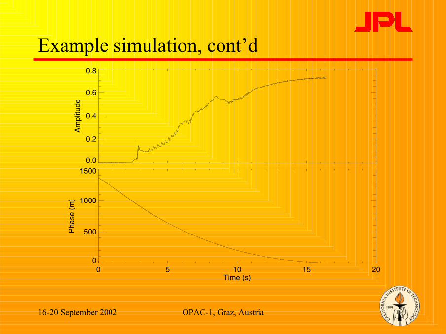
Example simulation, cont’d
0.0
0.2
0.4
0.6
0.8A
mpl
itude
0 5 10 15 20Time (s)
0
500
1000
1500
Pha
se (
m)
16-20 September 2002 OPAC-1, Graz, Austria 15
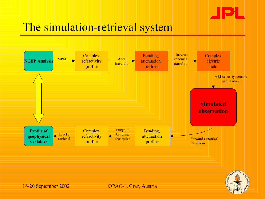
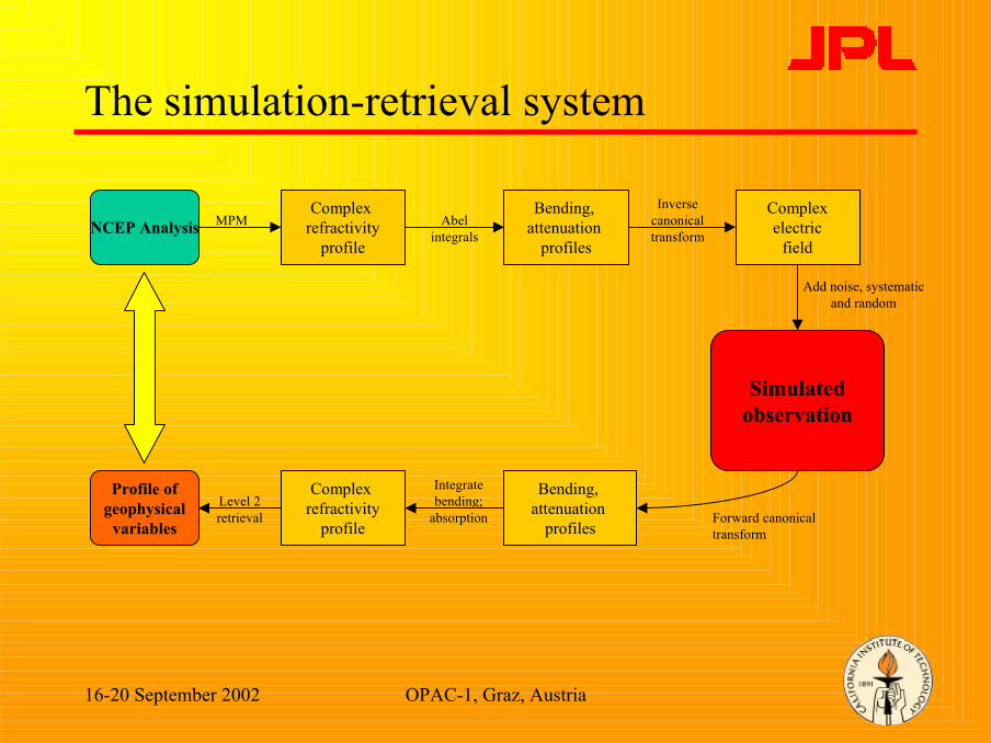
The simulation-retrieval system
NCEP AnalysisComplex
refractivityprofile
Simulatedobservation
Bending, attenuation
profiles
Complex refractivity
profile
Profile ofgeophysical
variables
MPMInverse
canonical transform
Add noise, systematicand random
Integrate bending;
absorptionLevel 2 retrieval
Bending, attenuation
profiles
Abel integrals
Forward canonical transform
Complexelectric
field
16-20 September 2002 OPAC-1, Graz, Austria 16
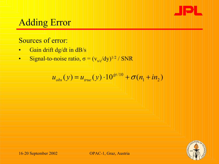
Adding Error
Sources of error:• Gain drift dg/dt in dB/s• Signal-to-noise ratio, σ = (vs/c/dy)1/2 / SNR
)(10)()( 2110/ innyuyu tg
trueobs ++⋅= σ&
16-20 September 2002 OPAC-1, Graz, Austria 17
The simulation-retrieval system
NCEP AnalysisComplex
refractivityprofile
Simulatedobservation
Bending, attenuation
profiles
Complex refractivity
profile
Profile ofgeophysical
variables
MPMInverse
canonical transform
Add noise, systematicand random
Integrate bending;
absorptionLevel 2 retrieval
Bending, attenuation
profiles
Abel integrals
Forward canonical transform
Complexelectric
field
16-20 September 2002 OPAC-1, Graz, Austria 18
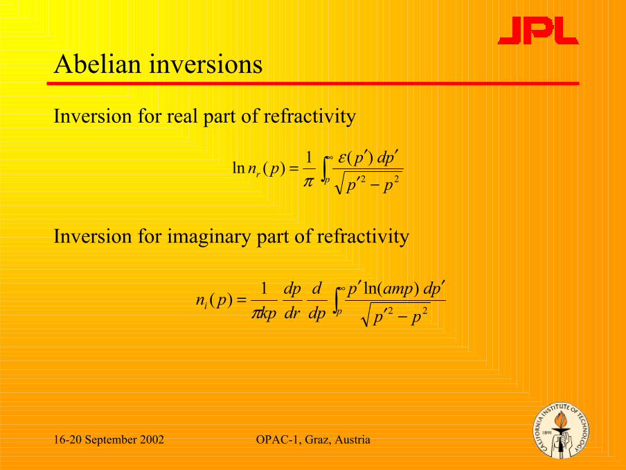
Abelian inversions
Inversion for real part of refractivity
Inversion for imaginary part of refractivity
∫∞
−′′′
=pr
pppdppn
22
)(1)(ln επ
∫∞
−′′′
=pi
pppdampp
dpd
drdp
kppn
22
)ln(1)(π
16-20 September 2002 OPAC-1, Graz, Austria 19
The simulation-retrieval system
NCEP AnalysisComplex
refractivityprofile
Simulatedobservation
Bending, attenuation
profiles
Complex refractivity
profile
Profile ofgeophysical
variables
MPMInverse
canonical transform
Add noise, systematicand random
Integrate bending;
absorptionLevel 2 retrieval
Bending, attenuation
profiles
Abel integrals
Forward canonical transform
Complexelectric
field
16-20 September 2002 OPAC-1, Graz, Austria 20
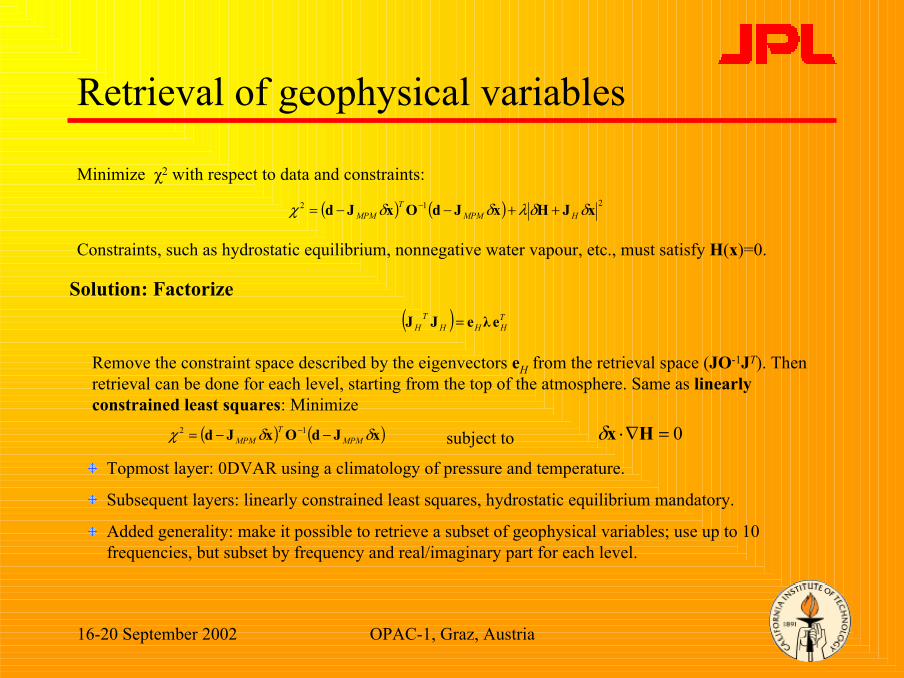
Retrieval of geophysical variables
Constraints, such as hydrostatic equilibrium, nonnegative water vapour, etc., must satisfy H(x)=0.
( ) ( ) 212 xJHxJdOxJd δδλδδχ HMPMT
MPM ++−−= −
Minimize χ2 with respect to data and constraints:
Solution: Factorize( ) T
HHHT
H eλeJJ =
Remove the constraint space described by the eigenvectors eH from the retrieval space (JO-1JT). Then retrieval can be done for each level, starting from the top of the atmosphere. Same as linearly constrained least squares: Minimize
Topmost layer: 0DVAR using a climatology of pressure and temperature.
Subsequent layers: linearly constrained least squares, hydrostatic equilibrium mandatory.
Added generality: make it possible to retrieve a subset of geophysical variables; use up to 10 frequencies, but subset by frequency and real/imaginary part for each level.
( ) ( )xJdOxJd δδχ MPMT
MPM −−= −12 subject to 0=∇⋅ Hxδ
16-20 September 2002 OPAC-1, Graz, Austria 21
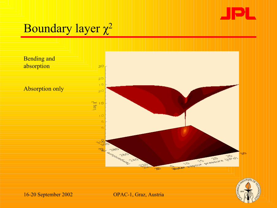
Boundary layer χ2
Bending and absorption
Absorption only
16-20 September 2002 OPAC-1, Graz, Austria 22
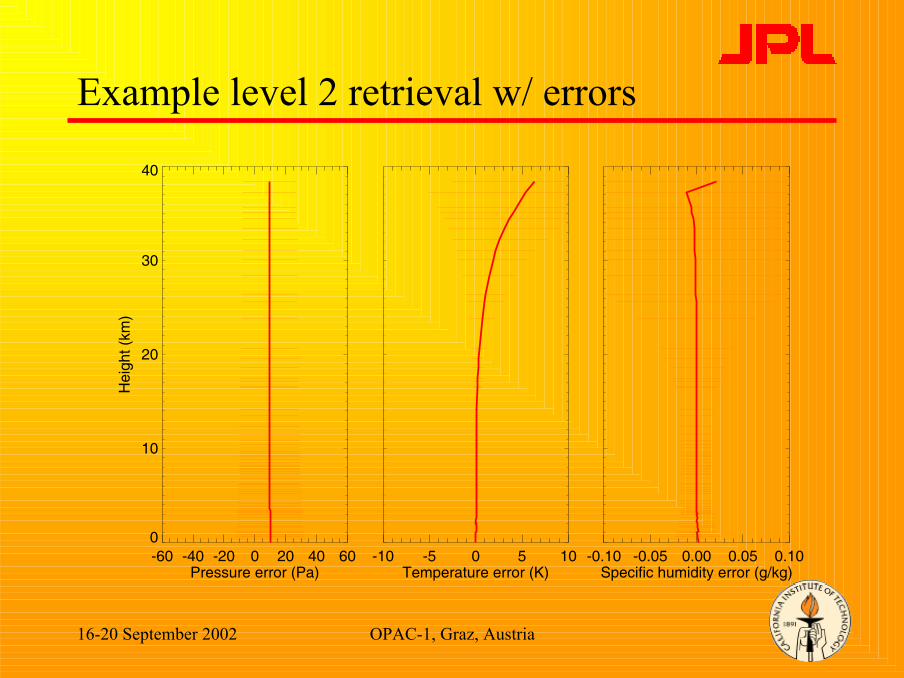
Example level 2 retrieval w/ errors
-60 -40 -20 0 20 40 60Pressure error (Pa)
0
10
20
30
40
Hei
ght (
km)
-10 -5 0 5 10Temperature error (K)
-0.10 -0.05 0.00 0.05 0.10Specific humidity error (g/kg)
16-20 September 2002 OPAC-1, Graz, Austria 23
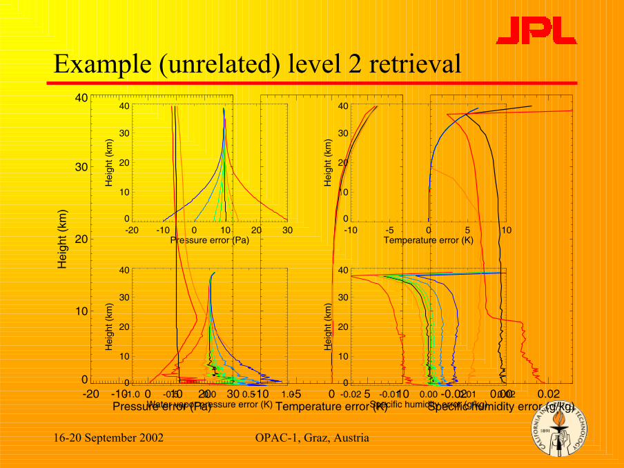
Example (unrelated) level 2 retrieval
-20 -10 0 10 20 30Pressure error (Pa)
0
10
20
30
40H
eigh
t (km
)
-10 -5 0 5 10Temperature error (K)
0
10
20
30
40
Hei
ght (
km)
-1.0 -0.5 0.0 0.5 1.0Water vapor pressure error (K)
0
10
20
30
40
Hei
ght (
km)
-0.02 -0.01 0.00 0.01 0.02Specific humidity error (g/kg)
0
10
20
30
40
Hei
ght (
km)
-20 -10 0 10 20 30Pressure error (Pa)
0
10
20
30
40
Hei
ght (
km)
-10 -5 0 5 10Temperature error (K)
-0.02 0.00 0.02Specific humidity error (g/kg)
16-20 September 2002 OPAC-1, Graz, Austria 24
Summary/Work-to-be-done
• Complete forward and inverse canonical transform• Include line parameterizations for ozone• Series of runs at 10.3, 17.2, 22.6 GHz• Series of runs with a “calibration tone” (3-5 GHz)• Try different gain drifts (0.01-0.10 dB/30s) with and
without calibration tone to determine how much the calibration tone helps
• Different SNRs (100-1000) with different sets of frequencies to determine sensitivity in the presence of clouds