Sound Morphing

XpertSolver.com

Contents Introduction ............................................................................................................................................ 1

Algorithm description ............................................................................................................................. 1

Simulations and results ........................................................................................................................... 2

Spectrogram: ....................................................................................................................................... 2

Conclusion ............................................................................................................................................... 5

References .............................................................................................................................................. 6

List of Figures Figure 1 Time domain plots of results with first carrier signal ............................................................... 2

Figure 2 Spectrogram using the second carrier signal ............................................................................ 3

Figure 3 Time domain plots of results with second carrier signal .......................................................... 3

Figure 4 Spectrogram using the second carrier signal ........................................................................... 4

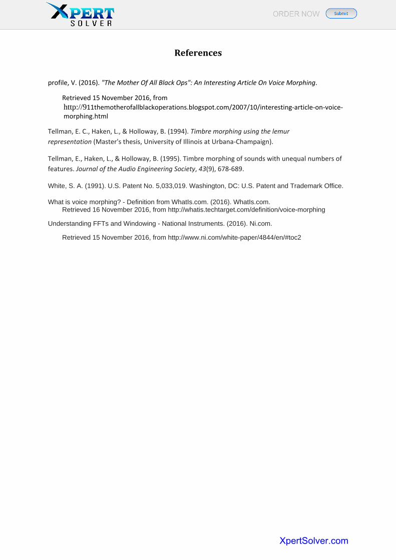
Figure 5 Spectrogram using the AWGN carrier signal ............................................................................ 5

List of Tables Table 1 Performance comparison ........................................................................................................... 4

XpertSolver.com

Introduction The project is based on the implementation of sound morphing on Matlab. Sound morphing is a computer generated alteration of human voice. This is accomplished by modulating (combining) human voice with some other sound. Different techniques are available for sound morphing. It can either be accomplished in time domain or frequency domain. Sound vocoding is another technique, similar to sound morphing which can be used to change the human voice

Sound morphing was originally developed at “Los Alamos National Laboratory” in New Mexico (Whatis , 2016). The researchers developed it for impersonating voices of number of USA generals. Early literature on sound morphing was published in IEEE. Notable initial work includes (Tellman et. al. , 1994) and (Tellman et. al. 1995).

In the past decade, sound morphing has been extensively applied in music and film industry. Other applications include impersonating different voices and generating realistic sounds of different musical instruments for entertainment purpose. Today, different sound morphing applications are available online for morphing human sound on computers as well as mobiles. Second life (Profile V. , 2016) is a notable morphing application for mobile platform while Voxal is often used on computers for morphing sounds.

Algorithm description

The algorithm essentially contains two input signals, the carrier signal and the modulating or voice signal. The function of the algorithm is to modulate the voice signal on the carrier signal. Hence the resulting signal will be the morphed and altered version of the voice signal. Windowing method is used for processing the signals. Windowing is done to divide the signal into small windows. Each window is then processed sequentially. FFT on a finite window size is known as SFFT. Windowing reduces the amplitude of the discontinuities in the data (White S. A. , 1991). Since window involves multiplication of the signal with time limited windows with smooth transition at the edges, it results in a smooth waveform without sharp transitions. Furthermore, windowing results in a better time resolution of the signal (Understanding FFTs , 2016).

Once STFT is taken of the windowed signals, the complex frequency vector of both signals is split into magnitude and spectrum. It must be noticed that only magnitude information is need for the voice signal. This is because the signal needs to be modulated on the carrier signal. Hence the resulting signal will acquire the frequency and phase of the carrier signal. Furthermore, the processing is only performed on the amplitude. The phase of the output signal remains unchanged. This is because, sound morphing only deals with changing amplitudes of signal at different frequencies. The magnitude of the voice signal fft is then normalized to limit the amplitude. It is accomplished by dividing the amplitude with the global average amplitude of the signal.

The final and foremost important step of morphing algorithm is to multiply the normalized voice magnitude in frequency domain with the carrier amplitude. Notice that the multiplication in frequency domain is equal to convolution in time domain. This gives us the idea that morphing is

XpertSolver.com

simply the spectral cross modulation or spectral convolution of two signals. The resultant magnitude and the phase of the system are utilized to take the inverse Fourier of the product signal.

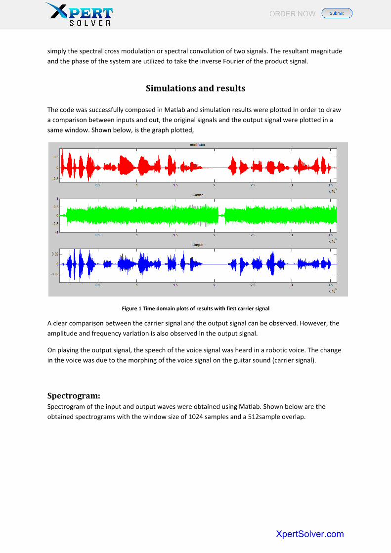
Simulations and results The code was successfully composed in Matlab and simulation results were plotted In order to draw a comparison between inputs and out, the original signals and the output signal were plotted in a same window. Shown below, is the graph plotted,

Figure 1 Time domain plots of results with first carrier signal

A clear comparison between the carrier signal and the output signal can be observed. However, the amplitude and frequency variation is also observed in the output signal.

On playing the output signal, the speech of the voice signal was heard in a robotic voice. The change in the voice was due to the morphing of the voice signal on the guitar sound (carrier signal).

Spectrogram: Spectrogram of the input and output waves were obtained using Matlab. Shown below are the obtained spectrograms with the window size of 1024 samples and a 512sample overlap.

XpertSolver.com

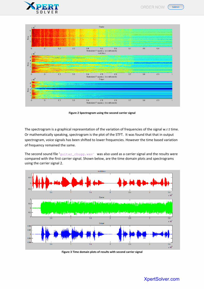
Figure 2 Spectrogram using the second carrier signal

The spectrogram is a graphical representation of the variation of frequencies of the signal w.r.t time. Or mathematically speaking, spectrogram is the plot of the STFT. It was found that that in output spectrogram, voice signals has been shifted to lower frequencies. However the time based variation of frequency remained the same.

The second sound file ‘guitar_chugg.wav' was also used as a carrier signal and the results were compared with the first carrier signal. Shown below, are the time domain plots and spectrograms using the carrier signal 2.

Figure 3 Time domain plots of results with second carrier signal

XpertSolver.com

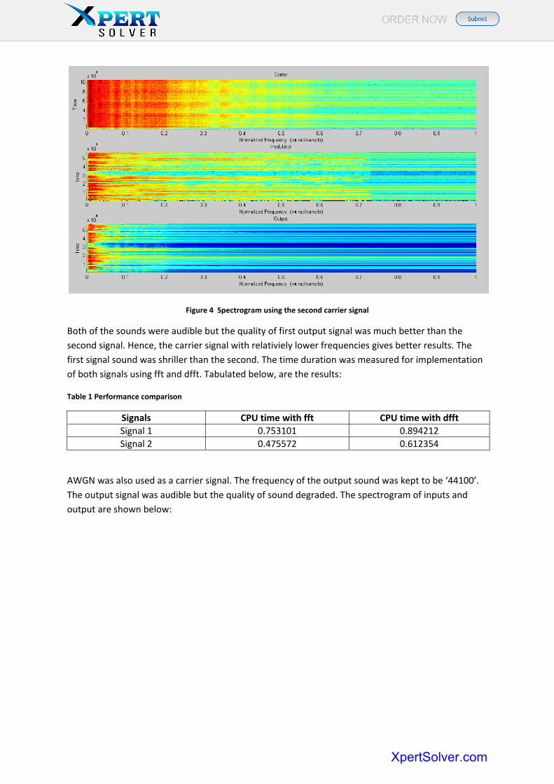
Figure 4 Spectrogram using the second carrier signal

Both of the sounds were audible but the quality of first output signal was much better than the second signal. Hence, the carrier signal with relativiely lower frequencies gives better results. The first signal sound was shriller than the second. The time duration was measured for implementation of both signals using fft and dfft. Tabulated below, are the results:

Table 1 Performance comparison

Signals CPU time with fft CPU time with dfft Signal 1 0.753101 0.894212 Signal 2 0.475572 0.612354

AWGN was also used as a carrier signal. The frequency of the output sound was kept to be ‘44100’. The output signal was audible but the quality of sound degraded. The spectrogram of inputs and output are shown below:

XpertSolver.com

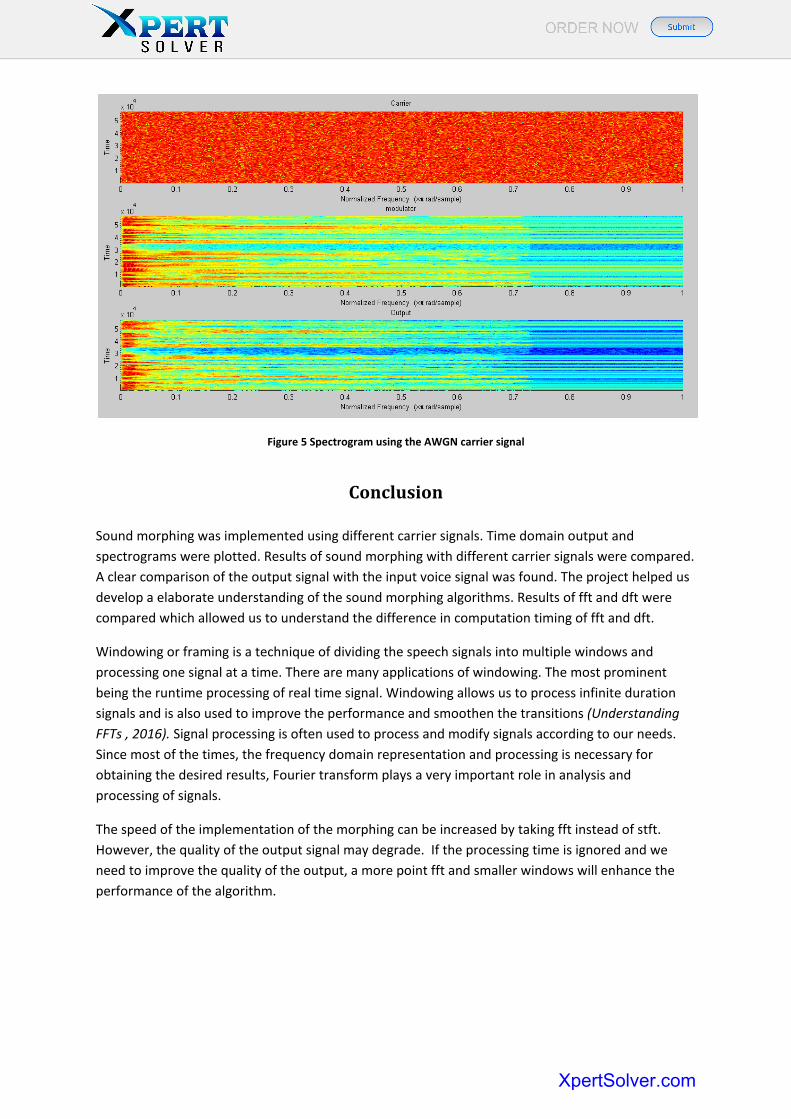
Figure 5 Spectrogram using the AWGN carrier signal

Conclusion Sound morphing was implemented using different carrier signals. Time domain output and spectrograms were plotted. Results of sound morphing with different carrier signals were compared. A clear comparison of the output signal with the input voice signal was found. The project helped us develop a elaborate understanding of the sound morphing algorithms. Results of fft and dft were compared which allowed us to understand the difference in computation timing of fft and dft.

Windowing or framing is a technique of dividing the speech signals into multiple windows and processing one signal at a time. There are many applications of windowing. The most prominent being the runtime processing of real time signal. Windowing allows us to process infinite duration signals and is also used to improve the performance and smoothen the transitions (Understanding FFTs , 2016). Signal processing is often used to process and modify signals according to our needs. Since most of the times, the frequency domain representation and processing is necessary for obtaining the desired results, Fourier transform plays a very important role in analysis and processing of signals.

The speed of the implementation of the morphing can be increased by taking fft instead of stft. However, the quality of the output signal may degrade. If the processing time is ignored and we need to improve the quality of the output, a more point fft and smaller windows will enhance the performance of the algorithm.

XpertSolver.com

References

profile, V. (2016). "The Mother Of All Black Ops": An Interesting Article On Voice Morphing.

Retrieved 15 November 2016, from http://911themotherofallblackoperations.blogspot.com/2007/10/interesting-article-on-voice-morphing.html

Tellman, E. C., Haken, L., & Holloway, B. (1994). Timbre morphing using the lemur representation (Master's thesis, University of Illinois at Urbana-Champaign).

Tellman, E., Haken, L., & Holloway, B. (1995). Timbre morphing of sounds with unequal numbers of features. Journal of the Audio Engineering Society, 43(9), 678-689.

White, S. A. (1991). U.S. Patent No. 5,033,019. Washington, DC: U.S. Patent and Trademark Office.

What is voice morphing? - Definition from WhatIs.com. (2016). WhatIs.com. Retrieved 16 November 2016, from http://whatis.techtarget.com/definition/voice-morphing

Understanding FFTs and Windowing - National Instruments. (2016). Ni.com.

Retrieved 15 November 2016, from http://www.ni.com/white-paper/4844/en/#toc2

XpertSolver.com

Appendix

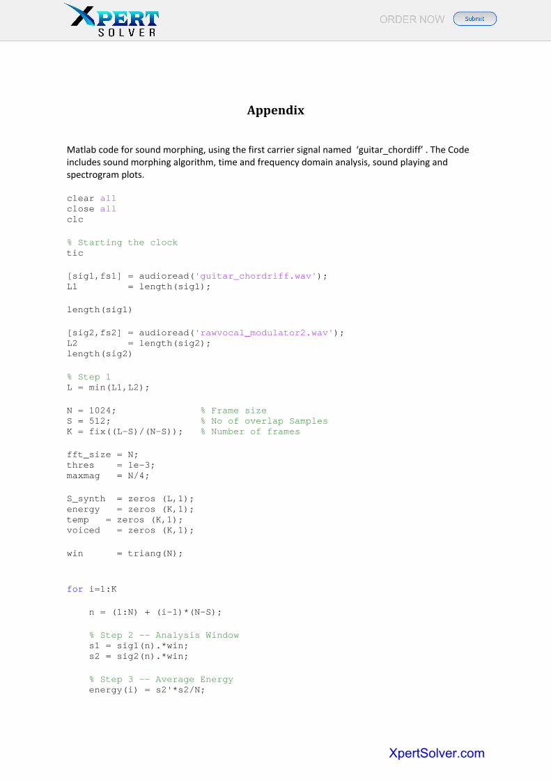
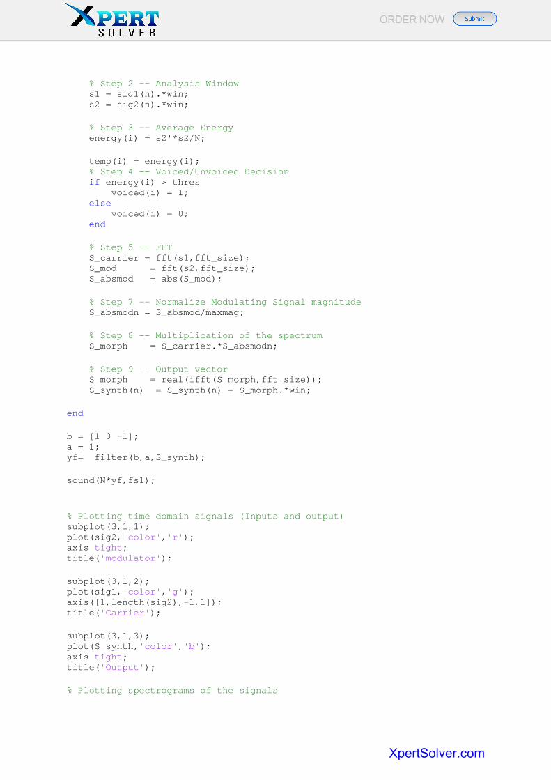
Matlab code for sound morphing, using the first carrier signal named ‘guitar_chordiff’ . The Code includes sound morphing algorithm, time and frequency domain analysis, sound playing and spectrogram plots. clear all close all clc % Starting the clock tic [sig1,fs1] = audioread('guitar_chordriff.wav'); L1 = length(sig1); length(sig1) [sig2,fs2] = audioread('rawvocal_modulator2.wav'); L2 = length(sig2); length(sig2) % Step 1 L = min(L1,L2); N = 1024; % Frame size S = 512; % No of overlap Samples K = fix((L-S)/(N-S)); % Number of frames fft_size = N; thres = 1e-3; maxmag = N/4; S_synth = zeros (L,1); energy = zeros (K,1); temp = zeros (K,1); voiced = zeros (K,1); win = triang(N); for i=1:K n = (1:N) + (i-1)*(N-S); % Step 2 -- Analysis Window s1 = sig1(n).*win; s2 = sig2(n).*win; % Step 3 -- Average Energy energy(i) = s2'*s2/N;

XpertSolver.com

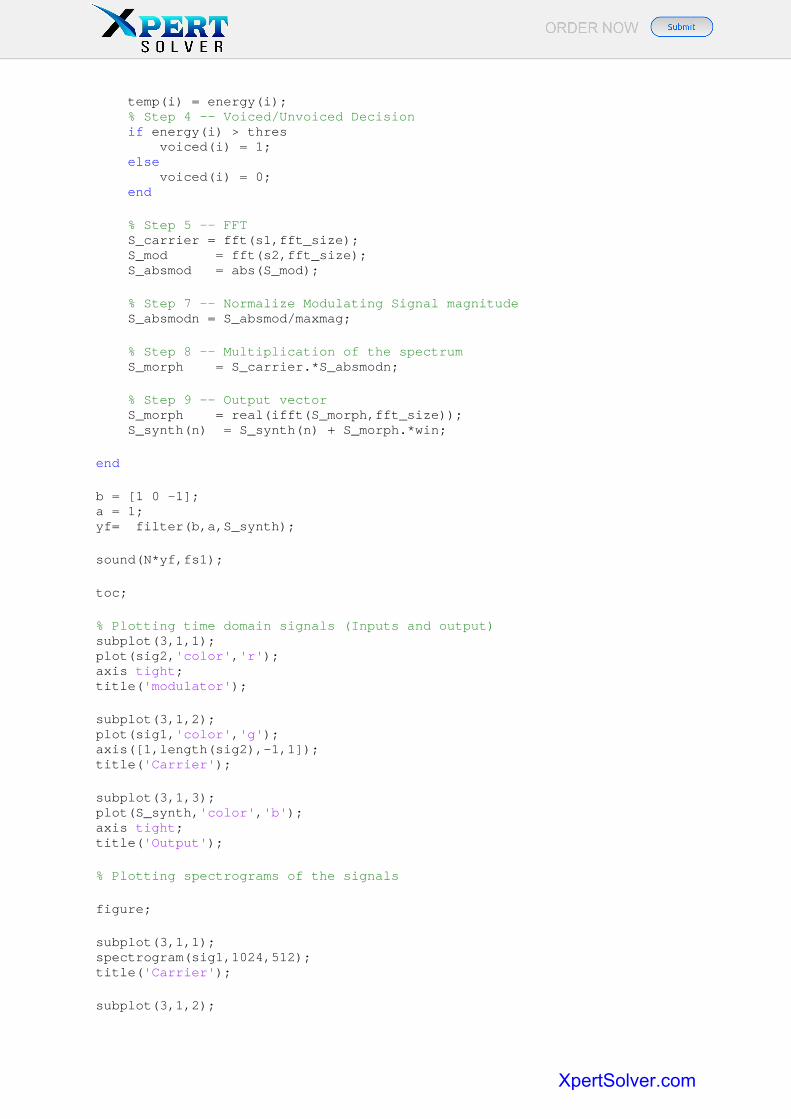
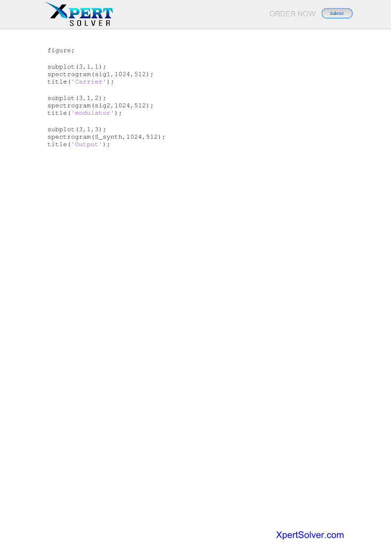
temp(i) = energy(i); % Step 4 -- Voiced/Unvoiced Decision if energy(i) > thres voiced(i) = 1; else voiced(i) = 0; end % Step 5 -- FFT S_carrier = fft(s1,fft_size); S_mod = fft(s2,fft_size); S_absmod = abs(S_mod); % Step 7 -- Normalize Modulating Signal magnitude S_absmodn = S_absmod/maxmag; % Step 8 -- Multiplication of the spectrum S_morph = S_carrier.*S_absmodn; % Step 9 -- Output vector S_morph = real(ifft(S_morph,fft_size)); S_synth(n) = S_synth(n) + S_morph.*win; end b = [1 0 -1]; a = 1; yf= filter(b,a,S_synth); sound(N*yf,fs1); toc; % Plotting time domain signals (Inputs and output) subplot(3,1,1); plot(sig2,'color','r'); axis tight; title('modulator'); subplot(3,1,2); plot(sig1,'color','g'); axis([1,length(sig2),-1,1]); title('Carrier'); subplot(3,1,3); plot(S_synth,'color','b'); axis tight; title('Output'); % Plotting spectrograms of the signals figure; subplot(3,1,1); spectrogram(sig1,1024,512); title('Carrier'); subplot(3,1,2);

XpertSolver.com

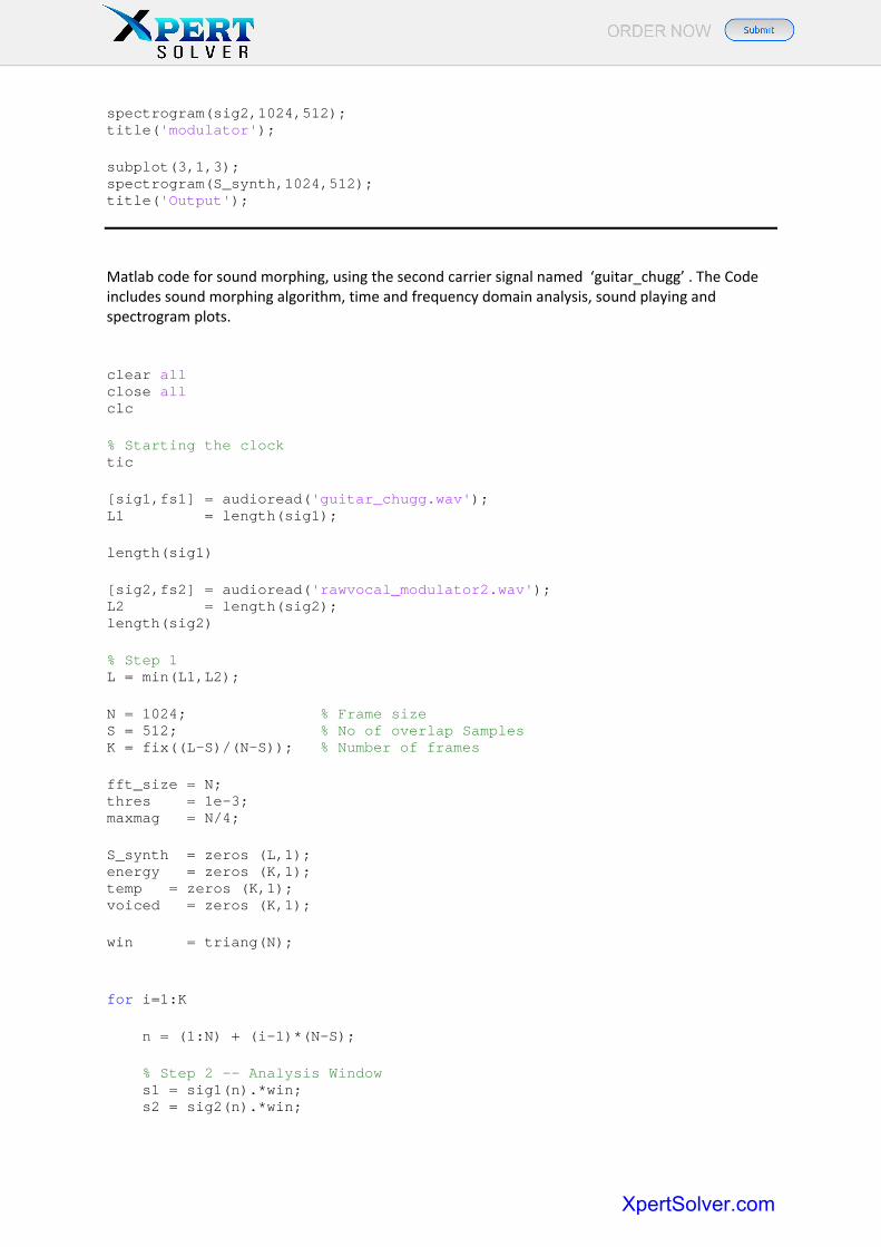
spectrogram(sig2,1024,512); title('modulator'); subplot(3,1,3); spectrogram(S_synth,1024,512); title('Output');

Matlab code for sound morphing, using the second carrier signal named ‘guitar_chugg’ . The Code includes sound morphing algorithm, time and frequency domain analysis, sound playing and spectrogram plots. clear all close all clc % Starting the clock tic [sig1,fs1] = audioread('guitar_chugg.wav'); L1 = length(sig1); length(sig1) [sig2,fs2] = audioread('rawvocal_modulator2.wav'); L2 = length(sig2); length(sig2) % Step 1 L = min(L1,L2); N = 1024; % Frame size S = 512; % No of overlap Samples K = fix((L-S)/(N-S)); % Number of frames fft_size = N; thres = 1e-3; maxmag = N/4; S_synth = zeros (L,1); energy = zeros (K,1); temp = zeros (K,1); voiced = zeros (K,1); win = triang(N); for i=1:K n = (1:N) + (i-1)*(N-S); % Step 2 -- Analysis Window s1 = sig1(n).*win; s2 = sig2(n).*win;

XpertSolver.com

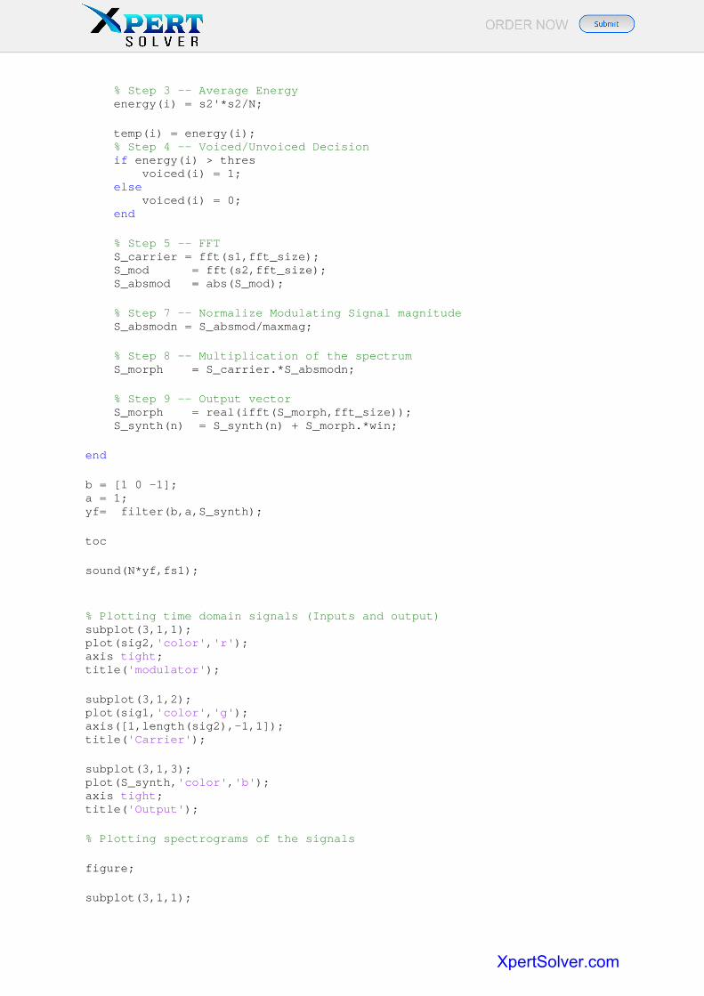
% Step 3 -- Average Energy energy(i) = s2'*s2/N; temp(i) = energy(i); % Step 4 -- Voiced/Unvoiced Decision if energy(i) > thres voiced(i) = 1; else voiced(i) = 0; end % Step 5 -- FFT S_carrier = fft(s1,fft_size); S_mod = fft(s2,fft_size); S_absmod = abs(S_mod); % Step 7 -- Normalize Modulating Signal magnitude S_absmodn = S_absmod/maxmag; % Step 8 -- Multiplication of the spectrum S_morph = S_carrier.*S_absmodn; % Step 9 -- Output vector S_morph = real(ifft(S_morph,fft_size)); S_synth(n) = S_synth(n) + S_morph.*win; end b = [1 0 -1]; a = 1; yf= filter(b,a,S_synth); toc sound(N*yf,fs1); % Plotting time domain signals (Inputs and output) subplot(3,1,1); plot(sig2,'color','r'); axis tight; title('modulator'); subplot(3,1,2); plot(sig1,'color','g'); axis([1,length(sig2),-1,1]); title('Carrier'); subplot(3,1,3); plot(S_synth,'color','b'); axis tight; title('Output'); % Plotting spectrograms of the signals figure; subplot(3,1,1);

XpertSolver.com

spectrogram(sig1,1024,512); title('Carrier'); subplot(3,1,2); spectrogram(sig2,1024,512); title('modulator'); subplot(3,1,3); spectrogram(S_synth,1024,512); title('Output');

Matlab code for sound morphing, using the stationary noise as a carrier signal . The Code includes sound morphing algorithm, time and frequency domain analysis, sound playing and spectrogram plots.

clear all close all clc sig1 = zeros(357825,1); sig1 = awgn(sig1,1); fs1 = 44100; L1 = length(sig1); length(sig1) [sig2,fs2] = audioread('rawvocal_modulator2.wav'); L2 = length(sig2); length(sig2) % Step 1 L = min(L1,L2); N = 1024; % Frame size S = 512; % No of overlap Samples K = fix((L-S)/(N-S)); % Number of frames fft_size = N; thres = 1e-3; maxmag = N/4; S_synth = zeros (L,1); energy = zeros (K,1); temp = zeros (K,1); voiced = zeros (K,1); win = triang(N); for i=1:K n = (1:N) + (i-1)*(N-S);

XpertSolver.com

% Step 2 -- Analysis Window s1 = sig1(n).*win; s2 = sig2(n).*win; % Step 3 -- Average Energy energy(i) = s2'*s2/N; temp(i) = energy(i); % Step 4 -- Voiced/Unvoiced Decision if energy(i) > thres voiced(i) = 1; else voiced(i) = 0; end % Step 5 -- FFT S_carrier = fft(s1,fft_size); S_mod = fft(s2,fft_size); S_absmod = abs(S_mod); % Step 7 -- Normalize Modulating Signal magnitude S_absmodn = S_absmod/maxmag; % Step 8 -- Multiplication of the spectrum S_morph = S_carrier.*S_absmodn; % Step 9 -- Output vector S_morph = real(ifft(S_morph,fft_size)); S_synth(n) = S_synth(n) + S_morph.*win; end b = [1 0 -1]; a = 1; yf= filter(b,a,S_synth); sound(N*yf,fs1); % Plotting time domain signals (Inputs and output) subplot(3,1,1); plot(sig2,'color','r'); axis tight; title('modulator'); subplot(3,1,2); plot(sig1,'color','g'); axis([1,length(sig2),-1,1]); title('Carrier'); subplot(3,1,3); plot(S_synth,'color','b'); axis tight; title('Output'); % Plotting spectrograms of the signals

XpertSolver.com

figure; subplot(3,1,1); spectrogram(sig1,1024,512); title('Carrier'); subplot(3,1,2); spectrogram(sig2,1024,512); title('modulator'); subplot(3,1,3); spectrogram(S_synth,1024,512); title('Output');

XpertSolver.com