some results on optimal control for nonlinear descriptor...
TRANSCRIPT
Linköping Studies in Science and TechnologyThesis No. 1227
Some Results On Optimal Control forNonlinear Descriptor Systems
Johan Sjöberg
REGLERTEKNIK
AUTOMATIC CONTROL
LINKÖPING
Division of Automatic ControlDepartment of Electrical Engineering
Linköpings universitet, SE-581 83 Linköping, Swedenhttp://www.control.isy.liu.se
Linköping 2006

This is a Swedish Licentiate’s Thesis.Swedish postgraduate education leads to a Doctor’s degree and/or a Licentiate’s degree. ADoctor’s Degree comprises 160 credits (4 years of full-time studies). A Licentiate’s degree
comprises 80 credits, of which at least 40 credits constitute a Licentiate’s thesis.
Some Results On Optimal Control for Nonlinear Descriptor Systems
c© 2006 Johan Sjöberg
Department of Electrical EngineeringLinköpings universitetSE-581 83 Linköping
Sweden
ISBN 91-85497-06-1 ISSN 0280-7971 LiU-TEK-LIC-2006:8
Printed by LiU-Tryck, Linköping, Sweden 2006

To Caroline!


Abstract
In this thesis, optimal feedback control for nonlinear descriptor systems is studied. Adescriptor system is a mathematical description that can include both differential andalgebraic equations. One of the reasons for the interest in this class of systems is thatseveral modern object-oriented modeling tools yield system descriptions in this form.Here, it is assumed that it is possible to rewrite the descriptor system as a state-spacesystem, at least locally. In theory, this assumption is not very restrictive because indexreduction techniques can be used to rewrite rather general descriptor systems to satisfythis assumption.
The Hamilton-Jacobi-Bellman equation can be used to calculate the optimal feedbackcontrol for systems in state-space form. For descriptor systems, a similar result existswhere a Hamilton-Jacobi-Bellman-like equation is solved. This equation includes an extraterm in order to incorporate the algebraic equations. Since the assumptions made heremake it possible to rewrite the descriptor system in state-space form, it is investigatedhow the extra term must be chosen in order to obtain the same solution from the differentequations.
A problem when computing the optimal feedback law using the Hamilton-Jacobi-Bellman equation is that it involves solving a nonlinear partial differential equation. Of-ten, this equation cannot be solved explicitly. An easier problem is to compute a locallyoptimal feedback law. This problem was solved in the 1960’s for analytical systems instate-space form and the optimal solution is described using power series. In this the-sis, this result is extended to also incorporate descriptor systems and it is applied to aphase-locked loop circuit.
In many situations, it is interesting to know if a certain region is reachable using somecontrol signal. For linear time-invariant state-space systems, this information is given bythe controllability gramian. For nonlinear state-space systems, the controllabilty functionis used instead. Three methods for calculating the controllability function for descriptorsystems are derived in this thesis. These methods are also applied to some examples inorder to illustrate the computational steps.
Furthermore, the observability function is studied. This function reflects the amountof output energy a certain initial state corresponds to. Two methods for calculating theobservability function for descriptor systems are derived. To describe one of the methods,a small example consisting of an electrical circuit is studied.
v

Sammanfattning
I denna avhandling studeras optimal återkopplad styrning av olinjära deskriptorsystem.Ett deskriptorsystem är en matematisk beskrivning som kan innehålla både differentia-lekvationer och algebraiska ekvationer. En av anledningarna till intresset för denna klassav system är att objekt-orienterade modelleringsverktyg ger systembeskrivningar på den-na form. Här kommer det att antas att det, åtminstone lokalt, är möjligt att eliminera dealgebraiska ekvationerna och få ett system på tillståndsform. Teoretiskt är detta inte såinskränkande för genom att använda någon indexreduktionsmetod kan ganska generelladeskriptorsystem skrivas om så att de uppfyller detta antagande.
För system på tillståndsform kan Hamilton-Jacobi-Bellman-ekvationen användas föratt bestämma den optimala återkopplingen. Ett liknande resultat finns för deskriptor-system där istället en Hamilton-Jacobi-Bellman-liknande ekvation ska lösas. Denna ek-vation innehåller dock en extra term för att hantera de algebraiska ekvationerna. Eftersomantagandena i denna avhandling gör det möjligt att skriva om deskriptorsystemet som etttillståndssystem, undersöks hur denna extra term måste väljas för att båda ekvationernaska få samma lösning.
Ett problem med att beräkna den optimala återkopplingen med hjälp av Hamilton-Jacobi-Bellman-ekvationen är att det leder till att en olinjär partiell differentialekvationska lösas. Generellt har denna ekvation ingen explicit lösning. Ett lättare problem är attberäkna en lokal optimal återkoppling. För analytiska system på tillståndsform löstes dettaproblem på 1960-talet och den optimala lösningen beskrivs av serieutvecklingar. I dennaavhandling generaliseras detta resultat så att även deskriptorsystem kan hanteras. Metodenillustreras med ett exempel som beskriver en faslåsande krets.
I många situationer vill man veta om ett område är möjligt att nå genom att styra pånågot sätt. För linjära tidsinvarianta system fås denna information från styrbarhetgramia-nen. För olinjära system används istället styrbarhetsfunktionen. Tre olika metoder för attberäkna styrbarhetsfunktionen har härletts i denna avhandling. De framtagna metodernaär också applicerade på några exempel för att visa beräkningsstegen.
Dessutom har observerbarhetsfunktionen studerats. Observerbarhetsfunktionen visarhur mycket utsignalenergi ett visst initial tillstånd svarar mot. Ett par olika metoder för attberäkna observerbarhetsfunktionen för deskriptorsystem tagits fram. För att beskriva enav metoderna, studeras ett litet exempel bestående av en elektrisk krets.
vii


Acknowledgments
First of all, I would like to thank my supervisor Professor Torkel Glad for introducingme to the interesting field of descriptor systems and for the skillful guidance during thework on this thesis. I have really enjoyed the cooperation so far and I look forward tothe continuation towards the next thesis. I would also like to thank Professor LennartLjung for letting me join the Automatic Control group in Linköping and for his excellentmanagement and support when needed. Ulla Salaneck also deserves extra gratitude forall administrative help and support.
I am really grateful to the persons that have proofread various parts of the thesis. Thesepersons are Lic. Daniel Axehill, Dr. Martin Enqvist, Lic. Markus Gerdin, Lic. GustafHendeby, Henrik Tidefelt, David Törnqvist, and Johan Wahlström.
I would like to thank the whole Automatic Control group for the kind and friendlyatmosphere. Being part of this group is a real pleasure.
There are some people which mean a lot also in the spare time. First, I would likethank Johan Wahlström, with whom I shared an apartment during my undergraduate stud-ies here in Linköping, and Daniel Axehill with whom I did the Master’s Thesis Project.During these years, we have had many nice discussions and good laughters together. Iwould also like to especially thank Martin Enqvist, Markus Gerdin, Gustaf Hendeby,Thomas Schön, Henrik Tidefelt, David Törnqvist, and Ragnar Wallin for putting up withall kinds of questions and for being really nice friends. Gustaf Hendeby also deservesextra appreciation for all help regarding LATEX. He is also the guy who have made the nicethesis style, in which this thesis is formatted.
I would also like to sincerely acknowledge all my friends from Kopparberg. It isalways a great pleasure to see all of you! Especially, I would like to thank Eva and MikaelNorwald for their kindness and generosity.
This work has been supported by the Swedish Research Council, and ECSEL (TheExcellence Center in Computer Science and Systems Engineering in Linköping), whichare hereby gratefully acknowledged.
Warm thanks are of course also dedicated to my parents, my brother and his wife forsupporting me and always being interested in what I am doing. Finally, I would like tothank Caroline for all the encouragement, support and love you give me. I love you!
Linköping, January 2006Johan Sjöberg
ix


Contents
1 Introduction 31.1 Thesis Outline . . . . . . . . . . . . . . . . . . . . . . . . . . . . . . . . 41.2 Contributions . . . . . . . . . . . . . . . . . . . . . . . . . . . . . . . . 4
2 Preliminaries 72.1 System Description . . . . . . . . . . . . . . . . . . . . . . . . . . . . . 72.2 System Index . . . . . . . . . . . . . . . . . . . . . . . . . . . . . . . . 9
2.2.1 Differential Index . . . . . . . . . . . . . . . . . . . . . . . . . . 102.2.2 Strangeness Index . . . . . . . . . . . . . . . . . . . . . . . . . 13
2.3 Solvability and Consistency . . . . . . . . . . . . . . . . . . . . . . . . . 132.4 Index Reduction . . . . . . . . . . . . . . . . . . . . . . . . . . . . . . . 21
2.4.1 Consecutive Differentiations . . . . . . . . . . . . . . . . . . . . 212.4.2 Consecutive Differentiations of Linear Time-Invariant Descriptor
Systems . . . . . . . . . . . . . . . . . . . . . . . . . . . . . . . 222.4.3 Kunkel and Mehrmann’s Method . . . . . . . . . . . . . . . . . 23
2.5 Stability . . . . . . . . . . . . . . . . . . . . . . . . . . . . . . . . . . . 262.5.1 Semi-Explicit Index One Systems . . . . . . . . . . . . . . . . . 272.5.2 Linear Systems . . . . . . . . . . . . . . . . . . . . . . . . . . . 312.5.3 Barrier Function Method . . . . . . . . . . . . . . . . . . . . . . 32
2.6 Optimal Control . . . . . . . . . . . . . . . . . . . . . . . . . . . . . . . 332.6.1 Formulation and Summary of the Optimal Control Problem . . . 332.6.2 Necessary Condition Using the HJB . . . . . . . . . . . . . . . . 342.6.3 Sufficient Condition Using HJB . . . . . . . . . . . . . . . . . . 362.6.4 Example . . . . . . . . . . . . . . . . . . . . . . . . . . . . . . 38
xi

xii Contents
3 Optimal Feedback Control for Descriptor Systems 413.1 Optimal Feedback Control . . . . . . . . . . . . . . . . . . . . . . . . . 423.2 Hamilton-Jacobi-Bellman Equation for the Reduced Problem . . . . . . . 433.3 Hamilton-Jacobi-Bellman-Like Equation . . . . . . . . . . . . . . . . . . 443.4 Relationships Among the Solutions . . . . . . . . . . . . . . . . . . . . . 453.5 Control-Affine Systems . . . . . . . . . . . . . . . . . . . . . . . . . . . 463.6 Example . . . . . . . . . . . . . . . . . . . . . . . . . . . . . . . . . . . 47
4 Power Series Solution of the Hamilton-Jacobi-Bellman Equation 494.1 Problem Formulation . . . . . . . . . . . . . . . . . . . . . . . . . . . . 504.2 Review of the State-Space System Case . . . . . . . . . . . . . . . . . . 514.3 Descriptor System Case . . . . . . . . . . . . . . . . . . . . . . . . . . . 54
4.3.1 Power Series Expansion of the Reduced Problem . . . . . . . . . 544.3.2 Application of the Results for State-Space Systems . . . . . . . . 564.3.3 Conditions on the Original Data . . . . . . . . . . . . . . . . . . 59
4.4 Extension . . . . . . . . . . . . . . . . . . . . . . . . . . . . . . . . . . 614.5 Example . . . . . . . . . . . . . . . . . . . . . . . . . . . . . . . . . . . 62
5 Controllability Function 675.1 Problem Formulation . . . . . . . . . . . . . . . . . . . . . . . . . . . . 685.2 Method Based on HJB Theory . . . . . . . . . . . . . . . . . . . . . . . 695.3 Method Based on Completion of Squares . . . . . . . . . . . . . . . . . 705.4 Method to Find a Local Solution . . . . . . . . . . . . . . . . . . . . . . 72
5.4.1 Basic Assumptions and Formulations . . . . . . . . . . . . . . . 725.4.2 Application of the Local Method . . . . . . . . . . . . . . . . . . 73
5.5 Linear Descriptor Systems . . . . . . . . . . . . . . . . . . . . . . . . . 765.6 Examples . . . . . . . . . . . . . . . . . . . . . . . . . . . . . . . . . . 78
5.6.1 Rolling Disc . . . . . . . . . . . . . . . . . . . . . . . . . . . . 785.6.2 Artificial System . . . . . . . . . . . . . . . . . . . . . . . . . . 805.6.3 Electrical Circuit . . . . . . . . . . . . . . . . . . . . . . . . . . 81
6 Observability Function 876.1 Problem Formulation . . . . . . . . . . . . . . . . . . . . . . . . . . . . 886.2 Method Based on Partial Differential Equation . . . . . . . . . . . . . . . 896.3 Method to Find a Local Solution . . . . . . . . . . . . . . . . . . . . . . 90
6.3.1 Basic Assumptions and Calculation of the Power Series Expan-sion of the Reduced System . . . . . . . . . . . . . . . . . . . . 90
6.3.2 Derivation of Power Series Method . . . . . . . . . . . . . . . . 916.4 Example . . . . . . . . . . . . . . . . . . . . . . . . . . . . . . . . . . . 92
7 Concluding Remarks 957.1 Conclusions . . . . . . . . . . . . . . . . . . . . . . . . . . . . . . . . . 957.2 Future work . . . . . . . . . . . . . . . . . . . . . . . . . . . . . . . . . 96
A Some Facts from Calculus and Set Theory 97
Bibliography 99
Notation
Symbols and Mathematical Notation
Notation MeaningRn the n-dimensional space of real numbersCn the n-dimensional space of complex numbers∈ belongs to∀ for allA ⊂ B A is a subset of BA ∩B the intersection between A and BA ∪B the union of A and B∂A the boundary of the set AIn the identity matrix of dimension n× nf : D → Q the function f maps a set D to a set Qf ∈ Ck(D,Q) a function f : D → Q is k-times continuously
differentiablefr;x the partial derivative of fr with respect to xQ () 0 the matrix Q is positive (semi)definiteQ ≺ () 0 the matrix Q is negative (semi)definiteσ(E,A) the set s ∈ C | det(sE −A) = 0λi(A) the ith eigenvalue of the matrix A< s the real part of s= s the imaginary part of sC+ the closed right half complex planeC− the open left half complex plane‖x‖
√xTx
minxf(x) minimization of f(x) with respect to x
argminx
f(x) the x minimizing f(x)
1
2 Notation
Notation MeaningBr the ball of radius r (see Appendix A)bxc the floor function, which gives the largest integer
less than or equal to xx time derivative of xx(i)(t) the ith derivative of x(t) with respect to tf [i](x) all terms in a multivariable polynomial of order io(h) f(h) = o(h) as h→ 0 if f(h)/h→ 0 as h→ 0corankA the rank deficiency of the matrix A with respect
to rows (see Appendix A)
AbbreviationsAbbreviation MeaningARE Algebraic Riccati EquationDAE Differential-Algebraic EquationDP Dynamic ProgrammingHJB Hamilton-Jacobi-Bellman (equation)HJI Hamilton-Jacobi InequalityODE Ordinary Differential EquationPLL Phase-Locked Loop circuitPMP Pontryagin Minimum Principle
Assumptions
Assumption Short explanationA1 The algebraic equations are possible to solve for
the algebraic variables, i.e., an implicit functionexists (see page 19)
A2 The set, on which the implicit function is defined,is global in the control input (see page 20)
A3 The index reduced system can be expressed insemi-explicit form (see page 25)
A4 The algebraic equations are locally possible tosolve for the algebraic variables (see page 51)
A5 The functions F1 and F2 for a semi-explicit de-scriptor system are analytical (see page 51)
A6 Only feedback laws locally stabilizing a descrip-tor system going backwards in time is considered(see page 73).
A7 The functions F1, F2 and h for a semi-explicitdescriptor system with an explicit output equa-tion are analytical (see page 90)
1Introduction
In real life, control strategies are used almost everywhere. Often these control strategiesform some kind of feedback control. This means that, based on observations, action istaken in order to obtain a certain goal. Which action to choose, given the actual observa-tions, is decided by the so-called controller. The controller can for example be a person, acomputer or a mechanical device. As an example, we can take one of the most well-knowncontrollers, namely the thermostat. The thermostat is used to control the temperature in aroom. Therefore, it measures the temperature in the room and if it is too high, the ther-mostat decreases the amount of hot water passing through the radiator, while if it is toolow, the amount is increased instead. In this way, the temperature of the room is kept at adesired level.
This very simple control strategy can in some cases be enough, but in many situationsbetter performance is desired. To achieve better performance it is most often necessaryto take the controlled system into consideration. This can of course be done in differentways, but in this thesis it will be assumed that we have a mathematical description ofthe system. The mathematical description is called a model of the system and the samesystem can be described by models in different forms.
One such form is the descriptor system form. The advantage with this form is that itallows for both differential and algebraic equations. This fact makes it possible to modelsystems in a very natural way in certain cases. One such case where the descriptor form isnatural to work with is when using object-oriented modeling methods. The basic idea inobject-oriented modeling is to create the complete model of a system as the compositionof many small models. To concretize we can use the modeling of a car as an example.
The first step is to model the engine, the gearbox, the propeller shaft, the car bodyetc. as separate models. The second step is to connect all the separate models to get themodel of the complete car. Typically, these connections will introduce algebraic equationsdescribing for example that the output shaft from the engine must to rotate with the sameangular velocity as the input shaft of the gearbox.
3

4 1 Introduction
Some examples where models in descriptor system form have been derived are forexample chemical processes (Kumar and Daoutidis, 1999), electrical circuits (Tischen-dorf, 2003), multibody mechanics in general (Hahn, 2002, 2003), multibody mechanicsapplied to a truck (Simeon et al., 1994; Rheinboldt and Simeon, 1999) and to robotics(McClamroch, 1990).
Supplied with a model in descriptor system form we consider controller design. Morespecifically optimal feedback control will be studied. Optimal feedback control meansthat the controller is designed to minimize a performance criterion. Therefore, the perfor-mance criterion should reflect the desired behavior of the controlled system. For example,for an engine management system, the performance criterion could be a combination ofthe fuel consumption and the difference between the actual torque delivered by the engineand the torque wanted by the driver. The design procedure would then yield the controllerachieving the best balance between low fuel consumption and delivery of the requestedtorque.
1.1 Thesis Outline
The thesis is separated into seven main chapters. Since the main subject of this work isdescriptor systems and optimal feedback control of such systems, Chapter 2 introducesthese subjects.
Chapter 3 is the first chapter devoted to optimal feedback control of descriptor sys-tems. Two different methods are investigated and some relationships between their opti-mal solutions are revealed. Chapter 4 deals with the same problem as Chapter 3, but inthis chapter the optimal feedback control problem is solved using series expansions. Themethod is very general but the solution might be restricted to a neighborhood.
The computation of the controllability function is considered in Chapter 5. The con-trollability function is defined as the solution to an optimal feedback control problem andtherefore the methods in Chapter 3 and Chapter 4 are used to solve this problem. Chap-ter 6 treats the computation of the observability function. The observability function isnot defined as the solution to an optimal feedback control problem, but it is still possibleto use ideas similar to those presented in Chapter 5.
Chapter 7 summarizes the thesis with some conclusions and remarks about interestingproblems for future research.
1.2 Contributions
The main contributions in this thesis are in the field of descriptor systems. This means thatwhen nothing else is mentioned, some control method for state-space systems is extendedto handle also descriptor systems.
A list of contributions, and the publications where these are presented, is given below.
• The analysis of the relationship among the solutions of two different methods forsolving the optimal feedback control problem, which can be found in Chapter 3.The presentation there is a modified version of the technical report:

1.2 Contributions 5
Glad, T. and Sjöberg, J. (2005). Optimal control for nonlinear descriptorsystems. Technical Report LiTH-ISY-R-2702, Department of ElectricalEngineering, Linköpings universitet.
• The method in Chapter 4 for finding a power series solution to the optimal feedbackcontrol problem. The material presented in this chapter comes from the conferencepaper:
Sjöberg, J. and Glad, T. (2005b). Power series solution of the Hamilton-Jacobi-Bellman equation for descriptor systems. In Proceedings of the44th IEEE Conference on Decision and Control, Seville, Spain.
The material has then been extended as described in Section 4.4.
• The different methods to compute the controllability function, given in Chapter 5.This chapter is based on results from:
Sjöberg, J. and Glad, T. (2005a). Computing the controllability functionfor nonlinear descriptor systems. Technical Report LiTH-ISY-R-2717,Department of Electrical Engineering, Linköpings universitet, SE-58183 Linköping, Sweden.
• The different methods in Chapter 6 to compute the observability function.
In addition to the contributions mentioned above, a small survey over theory for lineardescriptor systems has been published as a technical report:
Sjöberg, J. (2005). Descriptor systems and control theory. Technical Re-port LiTH-ISY-R-2688, Department of Electrical Engineering, Linköpingsuniversitet, SE-581 83 Linköping, Sweden

6 1 Introduction

2Preliminaries
To introduce the subject to the reader, we will in this chapter present some basic descriptorsystem theory. Four key concepts, index, solvability, consistency, and stability will bebriefly described. Furthermore, it will be discussed how the index of a system descriptioncan be lowered using some kind of index reduction method. Finally, an introduction tooptimal control of state-space systems will be given.
2.1 System Description
The original mathematical description of a system often consists of a set of differentialand algebraic equations. However, in most literature on control theory it is assumed thatthe algebraic equations can be used to eliminate some variables. The result is a systemdescription consisting only of differential equations that can be written in state-space formas
x = F (t, x, u) (2.1)
where x ∈ Rn is the state vector and u ∈ Rp is the control input. The state variablesrepresent the system’s memory of its past and throughout this thesis, a variable will onlybe denoted state if it has this property.
The state-space form has some drawbacks. For example, some systems are easy tomodel if both differential and algebraic equations may be used, while a reduction to astate-space model is more difficult. Another possible drawback occurs when the structureof the system description is nice and intuitive while using both kinds of equations, butthe state-space formulation looses some of these features. A third drawback is relatedto object-oriented computer modeling tools, such as Dymola. Usually, these tools do notyield system descriptions in state-space form, but as a set of both algebraic and differentialequations. In practice, the number of equations is often large and reduction to a state-space model is then almost impossible.
7
8 2 Preliminaries
Therefore, the focus of this thesis is at a more general class of model descriptions,called descriptor systems or differential-algebraic equations (DAE). This class of systemdescriptions includes both differential and algebraic equations and mathematically thiskind of system descriptions can be formulated as
F (t, x, x, u) = 0 (2.2)
where x ∈ Rn, u ∈ Rp and F : D → Rm for some set D ⊂ R2n+p+1. As for thestate-space model, u is here the control input. However, not all of the variables in x needto be states. The reason is that some components of x do not represent a memory of thepast, i.e., are not described by differential equations. This is shown in the following smallexample.
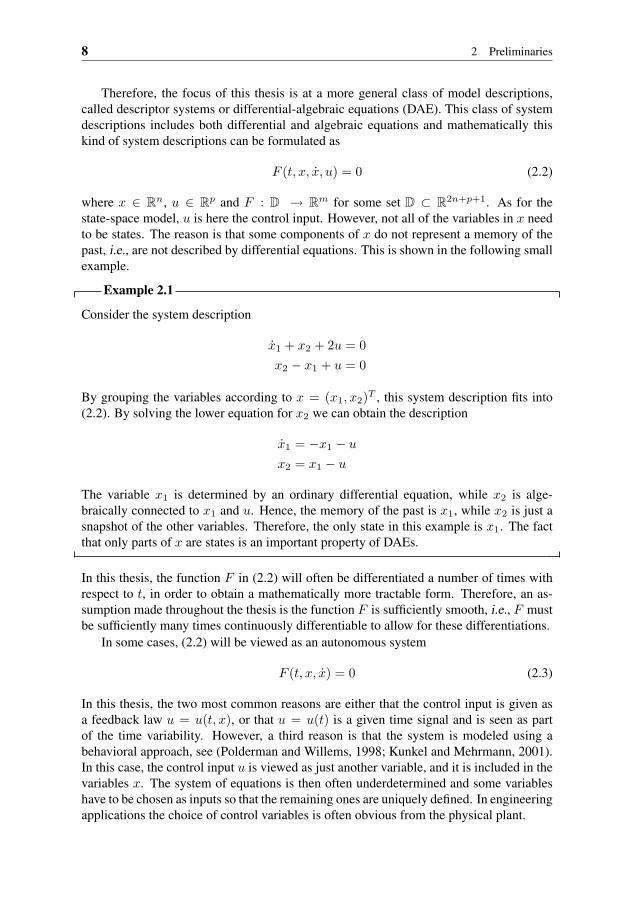
Example 2.1
Consider the system description
x1 + x2 + 2u = 0x2 − x1 + u = 0
By grouping the variables according to x = (x1, x2)T , this system description fits into(2.2). By solving the lower equation for x2 we can obtain the description
x1 = −x1 − u
x2 = x1 − u
The variable x1 is determined by an ordinary differential equation, while x2 is alge-braically connected to x1 and u. Hence, the memory of the past is x1, while x2 is just asnapshot of the other variables. Therefore, the only state in this example is x1. The factthat only parts of x are states is an important property of DAEs.
In this thesis, the function F in (2.2) will often be differentiated a number of times withrespect to t, in order to obtain a mathematically more tractable form. Therefore, an as-sumption made throughout the thesis is the function F is sufficiently smooth, i.e., F mustbe sufficiently many times continuously differentiable to allow for these differentiations.
In some cases, (2.2) will be viewed as an autonomous system
F (t, x, x) = 0 (2.3)
In this thesis, the two most common reasons are either that the control input is given asa feedback law u = u(t, x), or that u = u(t) is a given time signal and is seen as partof the time variability. However, a third reason is that the system is modeled using abehavioral approach, see (Polderman and Willems, 1998; Kunkel and Mehrmann, 2001).In this case, the control input u is viewed as just another variable, and it is included in thevariables x. The system of equations is then often underdetermined and some variableshave to be chosen as inputs so that the remaining ones are uniquely defined. In engineeringapplications the choice of control variables is often obvious from the physical plant.

2.2 System Index 9
Remark 2.1. Consider a system description (2.2) withm = n, i.e., with the same numberof equations as variables x. If the control input is a given signal, the system will have asmany unknowns in x as there are equations. However, for a behavioral model wherex and u are clustered and u is considered as just another variable, the system will beunderdetermined.
Often when modeling physical processes, the obtained system description will getmore structure than the general description (2.2). One such structure is the semi-explicitform. For example, this form naturally arises when modeling mechanical multibody sys-tems (Arnold et al., 2004), and it can be expressed as
Ex = F (x, u) (2.4)
where E ∈ Rn×n is a possibly rank deficient matrix, i.e., rankE = r ≤ n. Lineartime-invariant descriptor systems can always be written in this form as
Ex = Ax+Bu (2.5)
The description (2.4) (and hence (2.5)) can without loss of generality be written in semi-explicit form
x1 = F1(x1, x2, u) (2.6a)0 = F2(x1, x2, u) (2.6b)
where x1 ∈ Rr and x2 ∈ Rn−r. It may seem like all x1 are states, i.e., hold informationabout the past. However, as will be shown in the next section this does not need to be true,unless F2;x2(x1, x2, u) is at least locally nonsingular.
In some cases it might be interesting to extend the system descriptions above with anequation for an output signal y as
F (t, x, x, u) = 0 (2.7a)y = h(x, u) (2.7b)
where y ∈ Rq. In general, an explicit extension of the system with an extra output equa-tion is unnecessary for descriptor systems. Instead, the output equation can be includedin F (x, x, u, t) and the output signal y = y(t) is then seen as part of the time variability.However, in some situations it is important to show which variables that are possible tomeasure and in this case, (2.7) is the best system description.
2.2 System Index
The index is a commonly used concept in the theory of descriptor systems. Many differentkinds of indeces exist, for example differential index, perturbation index, strangenessindex. The common property of the different indices is that they in some sense measurehow different a given descriptor system is from a state-space system. Therefore, a systemdescription with high index will often be more difficult to handle than a description witha lower index. The index is mostly a model property and two different models in theform (2.2), modeling the same physical plant, can have different indices.
10 2 Preliminaries
In the sequel of this section, two kinds of indices, namely the differential index andthe strangeness index, will be discussed further. More information about different kindsof indices can be found in (Campbell and Gear, 1995; Kunkel and Mehrmann, 2001) andthe references therein.
2.2.1 Differential Index
The differential index is the most common of the different index concepts. It will alsobe this kind of index that in this thesis is denoted only the index. Loosely speaking, thedifferential index is the minimum number of differentiations needed to obtain an equiva-lent system of ordinary differential equations, i.e., a state-space system. A small exampleshowing the idea can be found below.
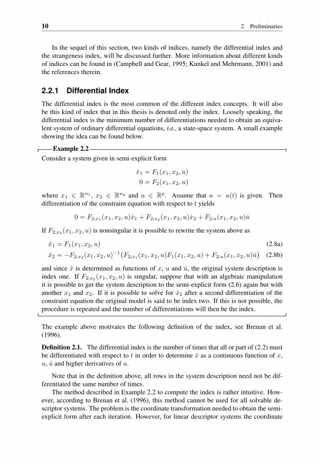
Example 2.2Consider a system given in semi-explicit form
x1 = F1(x1, x2, u)0 = F2(x1, x2, u)
where x1 ∈ Rn1 , x2 ∈ Rn2 and u ∈ Rp. Assume that u = u(t) is given. Thendifferentiation of the constraint equation with respect to t yields
0 = F2;x1(x1, x2, u)x1 + F2;x2(x1, x2, u)x2 + F2;u(x1, x2, u)u
If F2;x2(x1, x2, u) is nonsingular it is possible to rewrite the system above as
x1 = F1(x1, x2, u) (2.8a)
x2 = −F2;x2(x1, x2, u)−1(F2;x1(x1, x2, u)F1(x1, x2, u) + F2;u(x1, x2, u)u
)(2.8b)
and since x is determined as functions of x, u and u, the original system description isindex one. If F2;x2(x1, x2, u) is singular, suppose that with an algebraic manipulationit is possible to get the system description to the semi-explicit form (2.6) again but withanother x1 and x2. If it is possible to solve for x2 after a second differentiation of theconstraint equation the original model is said to be index two. If this is not possible, theprocedure is repeated and the number of differentiations will then be the index.
The example above motivates the following definition of the index, see Brenan et al.(1996).
Definition 2.1. The differential index is the number of times that all or part of (2.2) mustbe differentiated with respect to t in order to determine x as a continuous function of x,u, u and higher derivatives of u.
Note that in the definition above, all rows in the system description need not be dif-ferentiated the same number of times.
The method described in Example 2.2 to compute the index is rather intuitive. How-ever, according to Brenan et al. (1996), this method cannot be used for all solvable de-scriptor systems. The problem is the coordinate transformation needed to obtain the semi-explicit form after each iteration. However, for linear descriptor systems the coordinate
2.2 System Index 11
change is done using Gauss elimination. In this case, the method is called the Shufflealgorithm and was introduced by Luenberger (1978).
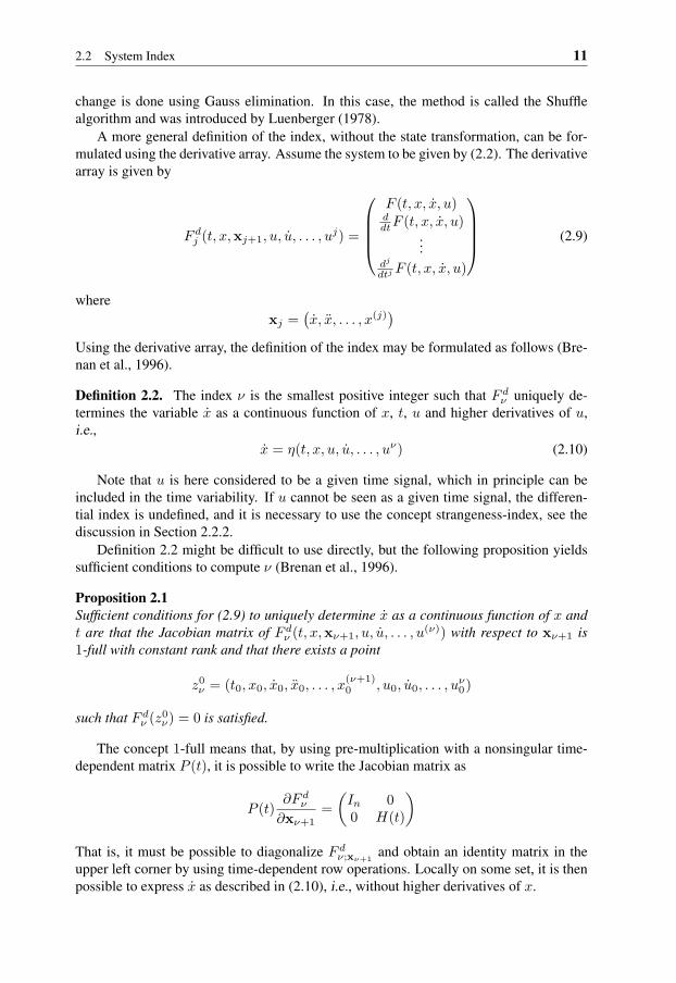
A more general definition of the index, without the state transformation, can be for-mulated using the derivative array. Assume the system to be given by (2.2). The derivativearray is given by
F dj (t, x,xj+1, u, u, . . . , u
j) =
F (t, x, x, u)ddtF (t, x, x, u)
...dj
dtj F (t, x, x, u)
(2.9)
wherexj =
(x, x, . . . , x(j)
)Using the derivative array, the definition of the index may be formulated as follows (Bre-nan et al., 1996).
Definition 2.2. The index ν is the smallest positive integer such that F dν uniquely de-
termines the variable x as a continuous function of x, t, u and higher derivatives of u,i.e.,
x = η(t, x, u, u, . . . , uν) (2.10)
Note that u is here considered to be a given time signal, which in principle can beincluded in the time variability. If u cannot be seen as a given time signal, the differen-tial index is undefined, and it is necessary to use the concept strangeness-index, see thediscussion in Section 2.2.2.
Definition 2.2 might be difficult to use directly, but the following proposition yieldssufficient conditions to compute ν (Brenan et al., 1996).
Proposition 2.1Sufficient conditions for (2.9) to uniquely determine x as a continuous function of x andt are that the Jacobian matrix of F d
ν (t, x,xν+1, u, u, . . . , u(ν)) with respect to xν+1 is
1-full with constant rank and that there exists a point
z0ν = (t0, x0, x0, x0, . . . , x
(ν+1)0 , u0, u0, . . . , u
ν0)
such that F dν (z0
ν) = 0 is satisfied.
The concept 1-full means that, by using pre-multiplication with a nonsingular time-dependent matrix P (t), it is possible to write the Jacobian matrix as
P (t)∂F d
ν
∂xν+1=(In 00 H(t)
)That is, it must be possible to diagonalize F d
ν;xν+1and obtain an identity matrix in the
upper left corner by using time-dependent row operations. Locally on some set, it is thenpossible to express x as described in (2.10), i.e., without higher derivatives of x.
12 2 Preliminaries
Remark 2.2. According to Brenan et al. (1996), nonlinear coordinate transformationsusing pre-multiplication by a nonsingular P (t) do not change the properties of constantrank or 1-fullness of the Jacobian matrix.
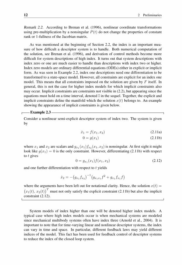
As was mentioned at the beginning of Section 2.2, the index is an important mea-sure of how difficult a descriptor system is to handle. Both numerical computation ofthe solution, see Brenan et al. (1996), and derivation of control methods become moredifficult for system descriptions of high index. It turns out that system descriptions withindex zero or one are much easier to handle than descriptions with index two or higher.Index zero models are ordinary differential equations (ODEs) either in explicit or implicitform. As was seen in Example 2.2, index one descriptions need one differentiation to betransformed to a state-space model. However, all constraints are explicit for an index onemodel. This means that all constraints imposed on the solution are given by F itself. Ingeneral, this is not the case for higher index models for which implicit constraints alsomay occur. Implicit constraints are constraints not visible in (2.2), but appearing since theequations must hold on a time interval, denoted I in the sequel. Together, the explicit andimplicit constraints define the manifold which the solution x(t) belongs to. An exampleshowing the appearance of implicit constraints is given below.
Example 2.3
Consider a nonlinear semi-explicit descriptor system of index two. The system is givenby
x1 = f(x1, x2) (2.11a)0 = g(x1) (2.11b)
where x1 and x2 are scalars and gx1(x1)fx2(x1, x2) is nonsingular. At first sight it mightlook like g(x1) = 0 is the only constraint. However, differentiating (2.11b) with respectto t gives
0 = gx1(x1)f(x1, x2) (2.12)
and one further differentiation with respect to t yields
x2 = −(gx1fx2
)−1(gx1x1f
2 + gx1fx1f)
where the arguments have been left out for notational clarity. Hence, the solution x(t) =(x1(t), x2(t)
)Tmust not only satisfy the explicit constraint (2.11b) but also the implicit
constraint (2.12).
System models of index higher than one will be denoted higher index models. Atypical case where high index models occur is when mechanical systems are modeledsince mechanical multibody systems often have index three (Arnold et al., 2004). It isimportant to note that for time-varying linear and nonlinear descriptor systems, the indexcan vary in time and space. In particular, different feedback laws may yield differentindices of the model. This fact has been used for feedback control of descriptor systemsto reduce the index of the closed loop system.

2.3 Solvability and Consistency 13
In some cases, the concept of differential index plays an important role also for state-space systems. One such case is the inversion problem where the objective is to find u interms of y and possibly x for a system
x = f(x, u)y = h(x, u)
(2.13)
where it is assumed that the number of inputs and outputs are the same. The procedures forinversion typically includes some differentiations, sometimes using Lie-bracket notation,until u can be recovered. The number of differentiations needed, is normally called therelative degree or order. However, for a given output signal y, the system (2.13) is adescriptor system in (x, u). The corresponding index of this descriptor system is therelative degree plus one.
2.2.2 Strangeness Index
Another index concept is the strangeness index µ, which for example is described inKunkel and Mehrmann (2001). The definition of the strangeness index will be presentedin the next section when solvability of descriptor systems is considered.
The strangeness index is a generalization of the differential index in the sense thatsome rank conditions are relaxed. Furthermore, unlike the differential index the strange-ness index is defined for over- and underdetermined system descriptions. However, forsystem descriptions where both the strangeness index and the differential index are well-defined the relation is, in principle, µ = max0, ν − 1. For a more thorough discussionabout this relationship the reader is referred to Kunkel and Mehrmann (1996). A systemwith µ = 0 is denoted strangeness-free.
2.3 Solvability and Consistency
Intuitively, solvability means that the descriptor system (2.2) possesses a well-behavedsolution. Well-behaved in this context means unique and sufficiently smooth, for examplecontinuously differentiable. For state-space systems, solvability follows if the systemsatisfies a Lipschitz condition, see Khalil (2002). For descriptor systems, the solvabilityproblem is somewhat more intrinsic.
In Section 2.2, it was shown that the solution of a descriptor system is, in principle,defined by the derivative array. If the index is finite, the derivative array can be solved forx and a solution can be computed by integration. However, for some systems the indexdoes not exist. Another complicating fact is the possibility of choosing initial conditionx(t0) such that the constraints are not satisfied. A third problem occurs when the controlsignal is not smooth enough and the solution contains derivatives of the control input.
The solvability definitions and theorems in this section are based on the results inKunkel and Mehrmann (1994, 1998, 2001). Other results on solvability for descriptorsystems can be found in (Brenan et al., 1996; Campbell and Gear, 1995; Campbell andGriepentrog, 1995). The method presented by Kunkel and Mehrmann (2001) also handlesunder- or overdetermined systems etc. An overdetermined system is a system wherethe number of equations m is larger than the number of unknowns, while the opposite
14 2 Preliminaries
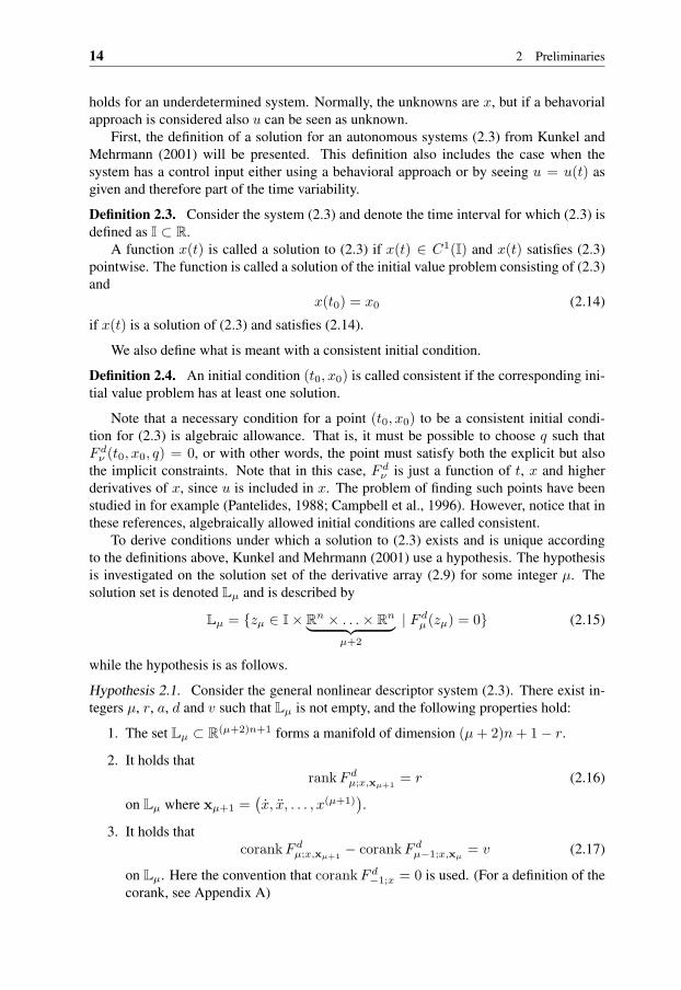
holds for an underdetermined system. Normally, the unknowns are x, but if a behavorialapproach is considered also u can be seen as unknown.
First, the definition of a solution for an autonomous systems (2.3) from Kunkel andMehrmann (2001) will be presented. This definition also includes the case when thesystem has a control input either using a behavioral approach or by seeing u = u(t) asgiven and therefore part of the time variability.
Definition 2.3. Consider the system (2.3) and denote the time interval for which (2.3) isdefined as I ⊂ R.
A function x(t) is called a solution to (2.3) if x(t) ∈ C1(I) and x(t) satisfies (2.3)pointwise. The function is called a solution of the initial value problem consisting of (2.3)and
x(t0) = x0 (2.14)
if x(t) is a solution of (2.3) and satisfies (2.14).
We also define what is meant with a consistent initial condition.
Definition 2.4. An initial condition (t0, x0) is called consistent if the corresponding ini-tial value problem has at least one solution.
Note that a necessary condition for a point (t0, x0) to be a consistent initial condi-tion for (2.3) is algebraic allowance. That is, it must be possible to choose q such thatF d
ν (t0, x0, q) = 0, or with other words, the point must satisfy both the explicit but alsothe implicit constraints. Note that in this case, F d
ν is just a function of t, x and higherderivatives of x, since u is included in x. The problem of finding such points have beenstudied in for example (Pantelides, 1988; Campbell et al., 1996). However, notice that inthese references, algebraically allowed initial conditions are called consistent.
To derive conditions under which a solution to (2.3) exists and is unique accordingto the definitions above, Kunkel and Mehrmann (2001) use a hypothesis. The hypothesisis investigated on the solution set of the derivative array (2.9) for some integer µ. Thesolution set is denoted Lµ and is described by
Lµ = zµ ∈ I× Rn × . . .× Rn︸ ︷︷ ︸µ+2
| F dµ (zµ) = 0 (2.15)
while the hypothesis is as follows.
Hypothesis 2.1. Consider the general nonlinear descriptor system (2.3). There exist in-tegers µ, r, a, d and v such that Lµ is not empty, and the following properties hold:
1. The set Lµ ⊂ R(µ+2)n+1 forms a manifold of dimension (µ+ 2)n+ 1− r.
2. It holds thatrankF d
µ;x,xµ+1= r (2.16)
on Lµ where xµ+1 =(x, x, . . . , x(µ+1)
).
3. It holds thatcorankF d
µ;x,xµ+1− corankF d
µ−1;x,xµ= v (2.17)
on Lµ. Here the convention that corankF d−1;x = 0 is used. (For a definition of the
corank, see Appendix A)

2.3 Solvability and Consistency 15
4. It holds thatrankF d
µ;xµ+1= r − a (2.18)
on Lµ such that there are smooth full rank matrix functions Z2 and T2 defined onLµ of size
((µ+ 1)m,a
)and (n, n− a), respectively, satisfying
ZT2 F
dµ;xµ+1
= 0, rankZT2 F
dµ;x = a, ZT
2 Fdµ;xT2 = 0 (2.19)
on Lµ.
5. It holds thatrankF d
xT2 = d = m− a− v (2.20)
on Lµ.
Note that the different ranks appearing in the hypothesis are assumed to be constanton the manifold Lµ.
If there exist µ, d, a and v such that the hypothesis above holds, it will imply thatthe system can be reduced to a system consisting of an implicit ODE and some algebraicequations. The implicit ODE forms d differential equations, while the number of algebraicequations are a. The motivation and procedure are described below. If the hypothesis isnot satisfied for a given µ, i.e., if d 6= m− a− v, µ is increased by one and the procedureis repeated. However, it is not certain that a µ exists such that the hypothesis hold.
The quantity v needs to be described. It measures the number of equations in theoriginal system (2.3) resulting in trivial equations 0 = 0, i.e., v measures the number ofredundant equations. Together with the numbers a and d, all m equations in the originalsystem are then characterized, since m = a+ d+ v.
The earlier mentioned strangeness index is also defined using Hypothesis 2.1. Thedefinition is as follows.
Definition 2.5. The strangeness index of (2.3) is the smallest positive integer µ such thatHypothesis 2.1 is satisfied.
The analysis of what the hypothesis implies is local and is done close to the pointz0µ = (t0, x0,xµ+1,0) ∈ Lµ where xµ+1,0 = (x0, . . . , x
(µ+1)0 ). The variables x(j)
0 wherej ≥ 1 are in this case seen as algebraic variables rather than as derivatives of x0. Frompart 1 of the hypothesis it is known that Lµ is a (µ+ 2)n+ 1− r dimensional manifold.Thus it is possible to locally parameterize it using (µ + 2)n + 1 − r parameters. Theseparameters can be chosen from (t, x,xµ+1) such that the rank of (2.21) is unchanged ifthe corresponding columns in
F dµ;x,xµ+1
(t0, x0,xµ+1,0) (2.21)
are removed. Together, parts 1 and 2 of the hypothesis give that
rankF dµ;t,x,xµ+1
= rankF dµ;x,xµ+1
= r
and hence t can be chosen as parameter. From part 2 it is also known that r variablesof (x,xµ+1) are determined (via the implicit function theorem) by the other (µ + 2)n +1 − r variables. From part 4, we have that r − a variables of xµ+1 are determined. We
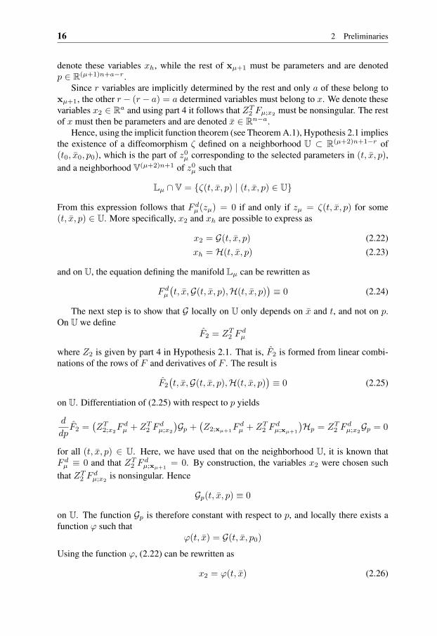
16 2 Preliminaries
denote these variables xh, while the rest of xµ+1 must be parameters and are denotedp ∈ R(µ+1)n+a−r.
Since r variables are implicitly determined by the rest and only a of these belong toxµ+1, the other r− (r− a) = a determined variables must belong to x. We denote thesevariables x2 ∈ Ra and using part 4 it follows that ZT
2 Fµ;x2 must be nonsingular. The restof x must then be parameters and are denoted x ∈ Rn−a.
Hence, using the implicit function theorem (see Theorem A.1), Hypothesis 2.1 impliesthe existence of a diffeomorphism ζ defined on a neighborhood U ⊂ R(µ+2)n+1−r of(t0, x0, p0), which is the part of z0
µ corresponding to the selected parameters in (t, x, p),and a neighborhood V(µ+2)n+1 of z0
µ such that
Lµ ∩ V = ζ(t, x, p) | (t, x, p) ∈ U
From this expression follows that F dµ (zµ) = 0 if and only if zµ = ζ(t, x, p) for some
(t, x, p) ∈ U. More specifically, x2 and xh are possible to express as
x2 = G(t, x, p) (2.22)xh = H(t, x, p) (2.23)
and on U, the equation defining the manifold Lµ can be rewritten as
F dµ
(t, x,G(t, x, p),H(t, x, p)
)≡ 0 (2.24)
The next step is to show that G locally on U only depends on x and t, and not on p.On U we define
F2 = ZT2 F
dµ
where Z2 is given by part 4 in Hypothesis 2.1. That is, F2 is formed from linear combi-nations of the rows of F and derivatives of F . The result is
F2
(t, x,G(t, x, p),H(t, x, p)
)≡ 0 (2.25)
on U. Differentiation of (2.25) with respect to p yields
d
dpF2 =
(ZT
2;x2F d
µ + ZT2 F
dµ;x2
)Gp +
(Z2;xµ+1F
dµ + ZT
2 Fdµ;xµ+1
)Hp = ZT
2 Fdµ;x2
Gp = 0
for all (t, x, p) ∈ U. Here, we have used that on the neighborhood U, it is known thatF d
µ ≡ 0 and that ZT2 F
dµ;xµ+1
= 0. By construction, the variables x2 were chosen suchthat ZT
2 Fdµ;x2
is nonsingular. Hence
Gp(t, x, p) ≡ 0
on U. The function Gp is therefore constant with respect to p, and locally there exists afunction ϕ such that
ϕ(t, x) = G(t, x, p0)
Using the function ϕ, (2.22) can be rewritten as
x2 = ϕ(t, x) (2.26)
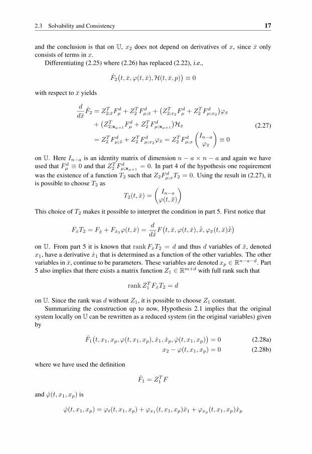
2.3 Solvability and Consistency 17
and the conclusion is that on U, x2 does not depend on derivatives of x, since x onlyconsists of terms in x.
Differentiating (2.25) where (2.26) has replaced (2.22), i.e.,
F2
(t, x, ϕ(t, x),H(t, x, p)
)≡ 0
with respect to x yields
d
dxF2 = ZT
2;xFdµ + ZT
2 Fdµ;x +
(ZT
2;x2F d
µ + ZT2 F
dµ;x2
)ϕx
+(ZT
2;xµ+1F d
µ + ZT2 F
dµ;xµ+1
)Hx
= ZT2 F
dµ;x + ZT
2 Fdµ;x2
ϕx = ZT2 F
dµ;x
(In−a
ϕx
)≡ 0
(2.27)
on U. Here In−a is an identity matrix of dimension n − a × n − a and again we haveused that F d
µ ≡ 0 and that ZT2 F
dµ;xµ+1
= 0. In part 4 of the hypothesis one requirementwas the existence of a function T2 such that Z2F
dµ;xT2 = 0. Using the result in (2.27), it
is possible to choose T2 as
T2(t, x) =(In−a
ϕ(t, x)
)This choice of T2 makes it possible to interpret the condition in part 5. First notice that
FxT2 = F ˙x + Fx3ϕ(t, x) =d
d ˙xF(t, x, ϕ(t, x), ˙x, ϕx(t, x) ˙x
)on U. From part 5 it is known that rankFxT2 = d and thus d variables of x, denotedx1, have a derivative x1 that is determined as a function of the other variables. The othervariables in x, continue to be parameters. These variables are denoted xp ∈ Rn−a−d. Part5 also implies that there exists a matrix function Z1 ∈ Rm+d with full rank such that
rankZT1 FxT2 = d
on U. Since the rank was d without Z1, it is possible to choose Z1 constant.Summarizing the construction up to now, Hypothesis 2.1 implies that the original
system locally on U can be rewritten as a reduced system (in the original variables) givenby
F1
(t, x1, xp, ϕ(t, x1, xp), x1, xp, ϕ(t, x1, xp)
)= 0 (2.28a)
x2 − ϕ(t, x1, xp) = 0 (2.28b)
where we have used the definition
F1 = ZT1 F
and ϕ(t, x1, xp) is
ϕ(t, x1, xp) = ϕt(t, x1, xp) + ϕx1(t, x1, xp)x1 + ϕxp(t, x1, xp)xp
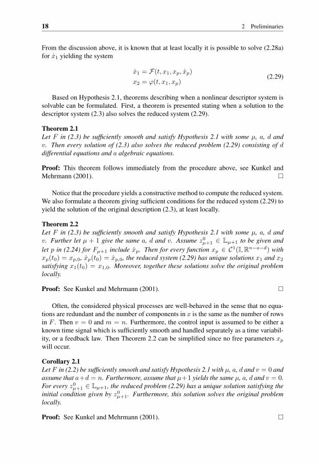
18 2 Preliminaries
From the discussion above, it is known that at least locally it is possible to solve (2.28a)for x1 yielding the system
x1 = F(t, x1, xp, xp)x2 = ϕ(t, x1, xp)
(2.29)
Based on Hypothesis 2.1, theorems describing when a nonlinear descriptor system issolvable can be formulated. First, a theorem is presented stating when a solution to thedescriptor system (2.3) also solves the reduced system (2.29).
Theorem 2.1Let F in (2.3) be sufficiently smooth and satisfy Hypothesis 2.1 with some µ, a, d andv. Then every solution of (2.3) also solves the reduced problem (2.29) consisting of ddifferential equations and a algebraic equations.
Proof: This theorem follows immediately from the procedure above, see Kunkel andMehrmann (2001).
Notice that the procedure yields a constructive method to compute the reduced system.We also formulate a theorem giving sufficient conditions for the reduced system (2.29) toyield the solution of the original description (2.3), at least locally.
Theorem 2.2Let F in (2.3) be sufficiently smooth and satisfy Hypothesis 2.1 with some µ, a, d andv. Further let µ + 1 give the same a, d and v. Assume z0
µ+1 ∈ Lµ+1 to be given andlet p in (2.24) for Fµ+1 include xp. Then for every function xp ∈ C1(I,Rn−a−d) withxp(t0) = xp,0, xp(t0) = xp,0, the reduced system (2.29) has unique solutions x1 and x2
satisfying x1(t0) = x1,0. Moreover, together these solutions solve the original problemlocally.
Proof: See Kunkel and Mehrmann (2001).
Often, the considered physical processes are well-behaved in the sense that no equa-tions are redundant and the number of components in x is the same as the number of rowsin F . Then v = 0 and m = n. Furthermore, the control input is assumed to be either aknown time signal which is sufficiently smooth and handled separately as a time variabil-ity, or a feedback law. Then Theorem 2.2 can be simplified since no free parameters xp
will occur.
Corollary 2.1Let F in (2.2) be sufficiently smooth and satisfy Hypothesis 2.1 with µ, a, d and v = 0 andassume that a+d = n. Furthermore, assume that µ+1 yields the same µ, a, d and v = 0.For every z0
µ+1 ∈ Lµ+1, the reduced problem (2.29) has a unique solution satisfying theinitial condition given by z0
µ+1. Furthermore, this solution solves the original problemlocally.
Proof: See Kunkel and Mehrmann (2001).
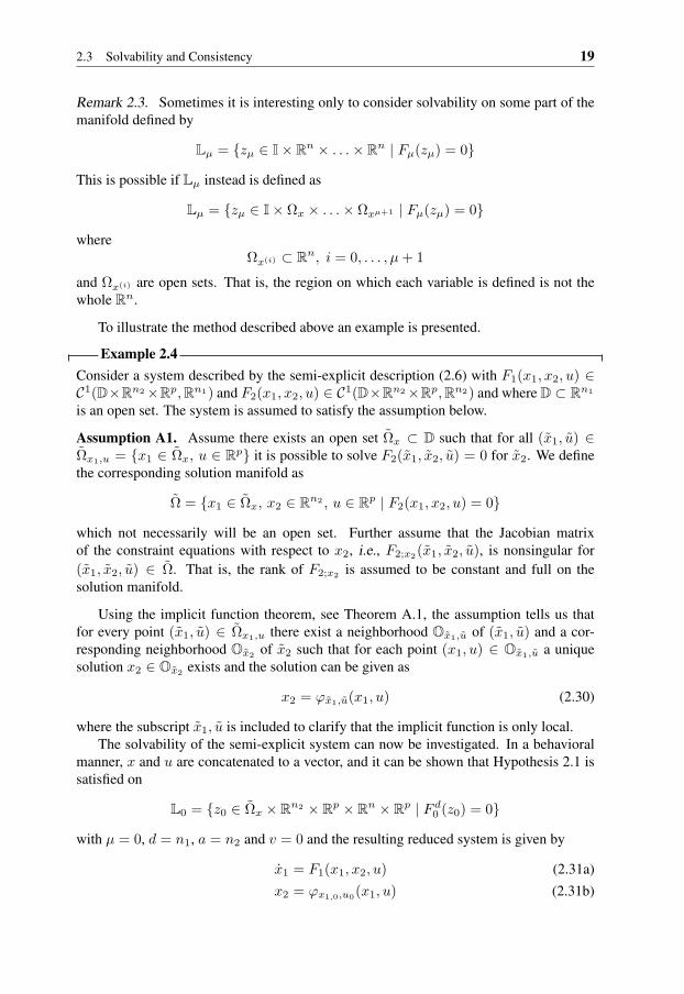
2.3 Solvability and Consistency 19
Remark 2.3. Sometimes it is interesting only to consider solvability on some part of themanifold defined by
Lµ = zµ ∈ I× Rn × . . .× Rn | Fµ(zµ) = 0
This is possible if Lµ instead is defined as
Lµ = zµ ∈ I× Ωx × . . .× Ωxµ+1 | Fµ(zµ) = 0
whereΩx(i) ⊂ Rn, i = 0, . . . , µ+ 1
and Ωx(i) are open sets. That is, the region on which each variable is defined is not thewhole Rn.
To illustrate the method described above an example is presented.
Example 2.4Consider a system described by the semi-explicit description (2.6) with F1(x1, x2, u) ∈C1(D×Rn2×Rp,Rn1) and F2(x1, x2, u) ∈ C1(D×Rn2×Rp,Rn2) and where D ⊂ Rn1
is an open set. The system is assumed to satisfy the assumption below.
Assumption A1. Assume there exists an open set Ωx ⊂ D such that for all (x1, u) ∈Ωx1,u = x1 ∈ Ωx, u ∈ Rp it is possible to solve F2(x1, x2, u) = 0 for x2. We definethe corresponding solution manifold as
Ω = x1 ∈ Ωx, x2 ∈ Rn2 , u ∈ Rp | F2(x1, x2, u) = 0
which not necessarily will be an open set. Further assume that the Jacobian matrixof the constraint equations with respect to x2, i.e., F2;x2(x1, x2, u), is nonsingular for(x1, x2, u) ∈ Ω. That is, the rank of F2;x2 is assumed to be constant and full on thesolution manifold.
Using the implicit function theorem, see Theorem A.1, the assumption tells us thatfor every point (x1, u) ∈ Ωx1,u there exist a neighborhood Ox1,u of (x1, u) and a cor-responding neighborhood Ox2 of x2 such that for each point (x1, u) ∈ Ox1,u a uniquesolution x2 ∈ Ox2 exists and the solution can be given as
x2 = ϕx1,u(x1, u) (2.30)
where the subscript x1, u is included to clarify that the implicit function is only local.The solvability of the semi-explicit system can now be investigated. In a behavioral
manner, x and u are concatenated to a vector, and it can be shown that Hypothesis 2.1 issatisfied on
L0 = z0 ∈ Ωx × Rn2 × Rp × Rn × Rp | F d0 (z0) = 0
with µ = 0, d = n1, a = n2 and v = 0 and the resulting reduced system is given by
x1 = F1(x1, x2, u) (2.31a)x2 = ϕx1,0,u0(x1, u) (2.31b)

20 2 Preliminaries
in some neighborhood of x1,0 and u0 which both belong to L0. Furthermore, it can beshown that the same d, a and v satisfy the hypothesis for µ = 1 on
L1 = z1 ∈ Ωx × Rn2 × Rp × Rn × Rp × Rn × Rp | F d1 (z1) = 0
and that the parameters p in F d1 can be chosen to include u. Given the initial conditions
(x1,0, x2,0, u0) ∈ Ω the initial conditions (x1,0, x2,0, x1,0, x2,0, u0) are possible to choosesuch that z0
1 ∈ L1. From Theorem 2.2 it then follows that for every continuously differ-entiable u(t) with u(t0) = u0, a unique solution exists for (2.31) such that x1(t0) = x1,0.Moreover, this solution locally solves the original system description.
Note that no u appear in the reduced system and therefore no initial condition u(t0) =u0 need to be specified when solving the system in practice.
In the sequel of this thesis, Assumption A1 will most often be combined with a secondassumption. Therefore, a combined assumption is formulated below.
Assumption A2. Assume that Assumption A1 is satisfied. Furthermore, assume thatone of the sets Ox1,u is global in u in the sense that it can be expressed as
Ox1,u = x1 ∈ Ωx, u ∈ Rp (2.32)
where Ωx is a neighborhood of x1 = 0.
For notational convenience in the sequel of the thesis, a corresponding set Ω is definedas
Ω = x1 ∈ Ωx, x2 ∈ Rn2 , u ∈ Rp |F2(x1, x2, u) = 0 (2.33)
on which the implicit function solving F2(x1, x2, u) = 0 is denoted
x2 = ϕ(x1, u), ∀x1 ∈ Ωx, u ∈ Rp (2.34)
For a linear descriptor system that is square, i.e., has as many equations as variablesx, the solvability conditions will reduce to the following theorem.
Theorem 2.3 (Solvability)Consider a linear time-invariant DAE
Ex = Ax+Bu
with regular sE−A, that is det(sE−A) 6≡ 0, and a given control signal u ∈ Cν(I,Rp).Then the system is solvable and every consistent initial condition yield a unique solution.
Proof: See Kunkel and Mehrmann (1994).
To simplify the notation in the sequel of the thesis, a linear time-invariant descriptorwith regular sE −A is denoted a regular system.
The definition of a solution for a general possibly nonlinear descriptor system requiresx(t) to be continuously differentiable. This is the classical requirement and for state-spacesystems (2.1) with a smooth enough system matrix F , it will basically impose the controlinput to be continuous.
2.4 Index Reduction 21
However, a continuous control input to a descriptor system will in certain cases notlead to a continuously differentiable solution. Even if the solution of the descriptor systemdoes not depend on derivatives of the control input, it is still a fact that the solution tothe algebraic part, i.e., x2 = ϕ(x1, u), can be only continuous since u can influencethe solution directly. Therefore, a more natural requirement on the solution might beto require the solution to the dynamical part to be continuously differentiable while thesolution to the algebraic part is allowed only to be continuous. In this case, continuouscontrol inputs can be used, if no derivatives of them appear.
One further generalization of the solution to state-space systems is that the solutiononly needs to be piecewise continuously differentiable. Then the control inputs are al-lowed to be only piecewise continuous, which is a rather common case, e.g., when usingcomputer generated signals. A natural extension of the solvability definition for descrip-tor systems would then be to require piecewise continuous differentiability of the solutionx1 to the dynamic part, while the solution x2 to the algebraic part only would need to bepiecewise continuous.
For linear time-invariant systems it is possible to relax the requirements even moreand define the solution in a distributional sense, see Dai (1989). With this framework,there exists a distributional solution even when the initial condition does not satisfy theexplicit and implicit constraints or when the control input is not sufficiently differentiable.For a more thorough discussion about distributional solutions, the reader is referred to Dai(1989), or the original works by Verghese (1978) and Cobb (1980).
2.4 Index Reduction
Index reduction is a procedure which takes a high index problem and rewrites it as alower index description, often index one or zero. Of course, the objective is to obtaina description that is easier to handle, and often also to reveal the manifold which thesolution must belong to. The key tool for lowering the index of a description and exposingthe implicit constraints is differentiation. Index reduction procedures are often the samemethods that are used either to compute the index of a system description or to showsolvability.
Numerical solvers for descriptor systems normally use index reduction methods inorder to obtain a system description of at most index one. The reason is that many nu-merical solvers are designed for index one descriptions (Brenan et al., 1996). Therefore,index reduction is a well-studied area, see, for example (Mattson and Söderlind, 1993;Kunkel and Mehrmann, 2004; Brenan et al., 1996) and the references therein.
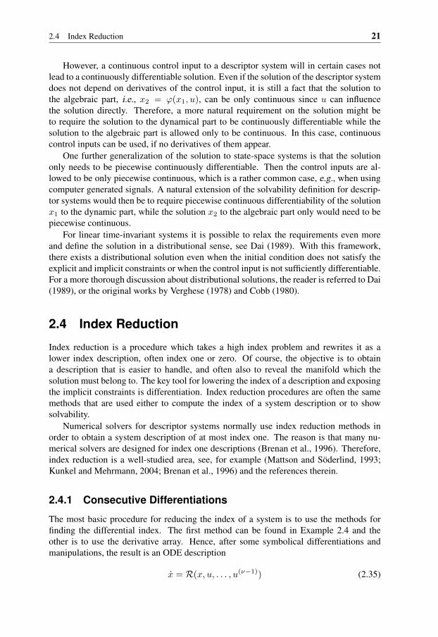
2.4.1 Consecutive Differentiations
The most basic procedure for reducing the index of a system is to use the methods forfinding the differential index. The first method can be found in Example 2.4 and theother is to use the derivative array. Hence, after some symbolical differentiations andmanipulations, the result is an ODE description
x = R(x, u, . . . , u(ν−1)) (2.35)
22 2 Preliminaries
The description (2.35) is equivalent to the original DAE in the sense that they yield thesame solution given consistent initial conditions. However, without considering the initialconditions, the solution manifold of (2.35) is much larger than for the original DAE. Toreduce the solution manifold and regain the same size as for the original problem theexplicit and implicit constraints, obtained in the index reduction procedure, need to beconsidered. For this purpose, the constraints can be used in different ways.
One way is to do as described above. That is, the constraints are used to define a setΩ0 and the initial condition x(t0) is then assumed to belong to this set, i.e., x(t0) ∈ Ω0.This way can be seen as a method to deal with the constraints implicitly. Another choiceis to augment the system description with the constraints as the index reduction procedureproceeds. The result is then an overdetermined but well-defined index one descriptorsystem. Theoretically, the choices are equivalent. However, in numerical simulation themethods have some differences.
A drawback with the first method is that it suffers from drift off, which often leadsto numerical instability. It means that even if the initial condition is chosen in Ω0, smallerrors in the numerical computations result in a solution to (2.35) which diverge from thesolution of the original descriptor system. This is a result of the larger solution set of(2.35) compared to the original system description. A solution to this problem is to usemethods known as constraint stabilization techniques (Baumgarte, 1972; Ascher et al.,1994).
For the second choice, the solution manifold is the same as for the original DAE.However, the numerical solver discretizes the problem and then according to Mattson andSöderlind (1993), an algebraically allowed point in the original DAE may be non-allowedin the discretized problem and vice versa. This problem can be handled using specialprojection methods, see references in Mattson and Söderlind (1993).
The problem with non-allowed points occurs because of the overdeterminedness ob-tained when all equations are augmented. Therefore, Mattson and Söderlind (1993)present another method where dummy derivatives are introduced. Extra variables areadded to the augmented system which instead of being overdetermined becomes deter-mined. The discretized problem will then be well-defined.
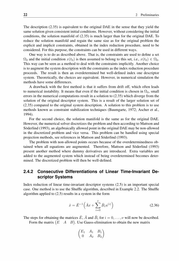
2.4.2 Consecutive Differentiations of Linear Time-Invariant De-scriptor Systems
Index reduction of linear time-invariant descriptor systems (2.5) is an important specialcase. One method is to use the Shuffle algorithm, described in Example 2.2. The Shufflealgorithm applied to (2.5) results in a system in the form
x = E−1(Ax+
ν∑i=0
Biu(i))
(2.36)
The steps for obtaining the matrices E, A and Bi for i = 0, . . . , ν will now be described.Form the matrix
(E A B
). Use Gauss-elimination to obtain the new matrix(
E1 A1 B1
0 A2 B2
)
2.4 Index Reduction 23
where E1 is nonsingular. This matrix corresponds to the descriptor system(E1
0
)x =
(A1
A2
)x+
(B1
B2
)u
Differentiation of the constraint equation, i.e., the lower row, yields the description(E1
−A2
)︸ ︷︷ ︸
E
x =(A1
0
)︸ ︷︷ ︸
A
x+(B1
0
)︸ ︷︷ ︸
B0
u+(
0B2
)︸ ︷︷ ︸
B1
u
If E has full rank, the description (2.36) is obtained by multiplying with the inverse ofE from the left. Otherwise, the procedure is repeated. The procedure is guaranteed toterminate if and only if the system is regular, see Dai (1989).
Another method with the advantage that it separates the dynamical and the algebraicparts is to use the canonical form. For linear descriptor systems (2.5), the canonical formis
x1 = A1x1 +B1u (2.37a)Nx2 = x2 +B2u (2.37b)
The matrix N is a nilpotent matrix, i.e., Nk = 0 for some integer k, and it can beproven that this k is the index of the system, i.e., k = ν (Brenan et al., 1996). A systemwith det(sE−A) 6≡ 0, can always be rewritten on this form and a computational methodto achieve this form can be found in Gerdin (2004).
Consecutive differentiations of the second row in the canonical form (2.37) will leadto that another form
x1 = A1x1 +B1u (2.38a)
x2 = −ν−1∑i=0
N iB2u(i)(t) (2.38b)
can be obtained. Here, it has been assumed that only consistent initial values x(0) areconsidered. The form (2.38) is widely used to show different properties for linear time-invariant descriptor systems, see Dai (1989).
Note that when the dynamical and algebraical parts of the original descriptor systemare separated like in (2.38), the numerical simulation becomes very simple. Only thedynamical part needs to be solved using an ODE solver, while the algebraic part is givenby the states and the control input. Therefore, no drift off or problems due to discretizationwill occur. This is a major advantage with this system description.
Results on a nonlinear version of the canonical form (2.37) can be found in Rouchonet al. (1992).
2.4.3 Kunkel and Mehrmann’s Method
The procedure presented in Section 2.3 when defining solvability for descriptor systemscan also be seen as an index reduction method. If µ, d, a and v are found such that
24 2 Preliminaries
Hypothesis 2.1 is satisfied, it is in principle possible to express the original description inthe form (2.29), i.e.,
x1 = F(t, x1, xp, xp)x2 = ϕ(t, x1, xp)
which has strangeness index zero. Unfortunately this description is only valid locallyin some neighborhood, and it might be impossible to find explicit expressions for thefunctions F and ϕ. However, the form above is obtained by solving the description
F1(t, x1, x2, xp, x1, xp, x2) = 0 (2.39a)
F2(t, x1, x2, xp) = 0 (2.39b)
with respect to x1 and x2, and (2.39) has also strangeness index zero. Unlike F and ϕ, itis often possible to express the functions F1 and F2 explicitly using the system function Fand possibly its derivatives (this is what the matrix functions Z1 and Z2 in Hypothesis 2.1do).
More practical aspects of the method described in this section can be found in Kunkeland Mehrmann (2004) and in Arnold et al. (2004).
Remark 2.4. For given µ, d, a and v the index reduction process is performed in onestep. Hence, no rank assumptions on intermediate steps are necessary. This may be anadvantage compared to other index reduction procedures.
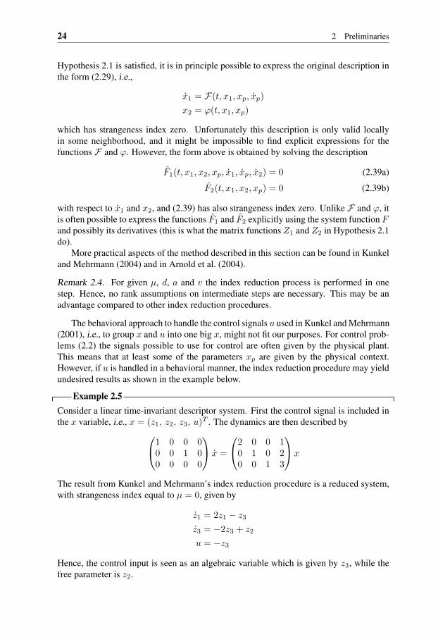
The behavioral approach to handle the control signals u used in Kunkel and Mehrmann(2001), i.e., to group x and u into one big x, might not fit our purposes. For control prob-lems (2.2) the signals possible to use for control are often given by the physical plant.This means that at least some of the parameters xp are given by the physical context.However, if u is handled in a behavioral manner, the index reduction procedure may yieldundesired results as shown in the example below.
Example 2.5Consider a linear time-invariant descriptor system. First the control signal is included inthe x variable, i.e., x = (z1, z2, z3, u)T . The dynamics are then described by1 0 0 0
0 0 1 00 0 0 0
x =
2 0 0 10 1 0 20 0 1 3
x
The result from Kunkel and Mehrmann’s index reduction procedure is a reduced system,with strangeness index equal to µ = 0, given by
z1 = 2z1 − z3
z3 = −2z3 + z2
u = −z3
Hence, the control input is seen as an algebraic variable which is given by z3, while thefree parameter is z2.

2.4 Index Reduction 25
In the next computation u is instead seen as a given signal, which is included in thetime variability. Hence, x = (z1, z2, z3), and the system description can be written as1 0 0
0 0 10 0 0
x =
2 0 00 1 00 0 1
x+
123
u
Applying the index reduction procedure on this description yields a dynamic part
z1 = 2z1 + u
z2 = −2u− 3uz3 = −3u
For this description µ = 1. Hence, by considering u as a given time signal, the strangenessindex has increased and u has appeared as a parameter.
The example above clearly shows that this index reduction procedure does not necessarilychoose the control input u as parameter.
Therefore, we will not use the behavioral approach and if the system (2.2) is handledwithout grouping x and u, and there exist µ, d, a and v such that Hypothesis 2.1 issatisfied, the functions F1 and F2 in (2.39) become
F1(t, x1, x2, x1, x2, u) = 0 (2.40a)
F2(x1, x2, u, u, . . . , u(µ)) = 0 (2.40b)
Since we assume that Hypothesis 2.1 is satisfied it is in principle possible, at least locally,to solve (2.40) for x1 and x2 to obtain
x1 = F(x1, u, . . . , u(µ+1)) (2.41a)
x2 = ϕ(x1, u, u, . . . , u(µ)) (2.41b)
The system above is in semi-explicit form (2.6), but as mentioned earlier it may be im-possible to find explicit expressions for F and ϕ. However, often in this thesis, it will beassumed that the system (2.40) can be written in semi-explicit form with system functionsF1 and F2 given in closed form. We formulate this assumption more formally.
Assumption A3. The variables x1 can be solved from (2.40a) to give
x1 = F1(x1, x2, u, . . . , u(µ+1)) (2.42a)
0 = F2(x1, x2, u, u, . . . , u(µ)) (2.42b)
where F1 and F2 are possible to express explicitly.
It may seem strange that x2 has disappeared in F1. However, differentiation of (2.42b)makes it is possible to get an expression for x2 as
x2 = −F−12;x2
(x1, x2,u)(F2;x1(x1, x2,u)x1 + F2;u(x1, x2,u)u
)
26 2 Preliminaries
where u = (u, u, . . . , u(µ)). Using this expression, x2 can be eliminated from F1.The class of applications where F1 actually is affine in x1 seems to be rather large.
For example mechanical multibody systems can in many cases be written in this form,see Kunkel and Mehrmann (2001).
One complication is the possible presence of derivatives of the control variable (orig-inating from differentiations of the equations). If the procedure is allowed to choose theinput signal, or with other words the parameter xp, freely the highest possible derivativeis xp. However, if the control input is chosen by the physical plant, the highest possiblederivative becomes u(µ+1). For linear systems, it is possible to make transformations re-moving the input derivatives from the differential equations and just have the derivativesin the algebraic part as can be seen in (2.38). This might not be possible in the nonlinearcase. In that case, it could be necessary to redefine the control signal so that its highestderivative becomes a new control variable and the lower order derivatives become statevariables. This procedure introduces an integrator chain
x1,n1+1 = x1,n1+2
...
x1,n1+µ+1 = u(µ+1)
If the integrator chain is included, the system description (2.42) becomes
x1 = F1(x1, x2, u) (2.43a)0 = F2(x1, x2, u) (2.43b)
where x1 ∈ Rn1+µ+1, x2 ∈ Rn2 and u ∈ Rp. Here u(µ+1) is denoted u in order tonotationally match the sequel of this thesis.
2.5 Stability
This section concerns stability analysis of descriptor systems. In principle, stability ofa descriptor system means stability of a dynamical system on a manifold. The standardtool, and basically the only tool, for proving stability for nonlinear systems is Lyapunovtheory. The main concept in the Lyapunov theory is the use of a Lyapunov function, seeLyapunov (1992). The Lyapunov function is in some sense a distance measure betweenthe variables x and an equilibrium point. If this distance measure decreases or at least isconstant, the state is not diverging from the equilibrium and stability can be concluded.
A practical problem with Lyapunov theory is that in many cases, a Lyapunov functioncan be difficult to find for a general nonlinear system. However, for mechanical andelectrical systems, often the total energy content of the system can be used.
The stability results will be focused on two system descriptions, the semi-explicit, au-tonomous, index one case and the linear case. These two cases will be the most importantfor the forthcoming chapters. However, a small discussion about polynomial possiblyhigher index systems will be presented at the end of this section. For this kind of systemsa computationally tractable approach, based on Lyapunov theory, has been published inEbenbauer and Allgöwer (2004).
2.5 Stability 27
Consider the autonomous descriptor system
F (x, x) = 0 (2.44)
where x ∈ Rn. This system can be thought of as either a system without control input oras a closed loop system with feedback u = u(x).
Assume that there exists an open connected set Ω of consistent initial conditions suchthat the solution is unique, i.e., the initial value problem consisting of (2.44) together withx(t0) ∈ Ω has a unique solution. Note that in the state-space case this assumption willsimplify to Ω being some subset of the domain where the system satisfies a Lipschitzcondition.
Stability is studied and characterized with respect to some equilibrium. Therefore, itis assumed that the system has an equilibrium x0 ∈ Ω. Without loss of generality theequilibrium can be assumed to be the origin, since if x0 6= 0, the change of variablesz = x− x0 can be used. In the equilibrium, (2.44) gives
0 = F (0, x0) = F (0, 0)
where F (z, z) = F (x, x). Hence, in the new variables z, the equilibrium has been shiftedto the origin.
Finally, the set Ω is assumed to contain only a single equilibrium. Hence, in order tosatisfy this assumption, it might be necessary to reduce Ω. However, this assumption canbe relaxed using concepts of set stability, see Hill and Mareels (1990).
The definitions of stability for descriptor systems are natural extensions of the corre-sponding definitions for the state-space case.
Definition 2.6 (Stability). The equilibrium point at (0, 0) of (2.44) is called stable ifgiven a ε > 0, there exists a δ(ε) > 0 such that for all x(t0) ∈ Ω ∩ Bδ it follows thatx(t) ∈ Ω ∩Bε, ∀t > 0.
Definition 2.7 (Asymptotic stability). The equilibrium point at (0, 0) of (2.44) is calledasymptotically stable if it is stable and there exists a η > 0 such that for all x(t0) ∈ Ω∩Bη
it follows thatlim
t→∞
∥∥x(t)∥∥ = 0
2.5.1 Semi-Explicit Index One Systems
Lyapunov stability for semi-explicit index one systems is a rather well-studied area, seefor example Hill and Mareels (1990), Wu and Mizukami (1994) and Wang et al. (2002). Inmany cases, using the index reduction method in Section 2.4.3 and by assuming that As-sumption A3 is satisfied, also higher index descriptions can be rewritten in semi-explicitform. Hence, we consider the case when (2.44) can be expressed as
x1 = F1(x1, x2) (2.45a)0 = F2(x1, x2) (2.45b)
where x1 ∈ Rn1 and x2 ∈ Rn2 . The system is assumed to satisfy Assumption A2. Thismeans that, on some set Ω, which in this case has the structure
Ω = x1 ∈ Ωx ⊂ Rn1 , x2 ∈ Rn2 , | x2 = ϕ(x1) (2.46)
28 2 Preliminaries
the system (2.45) has index one and a unique solution for arbitrary initial conditions in Ω.We also assume that Ω is connected and contains the origin.
Lyapunov’s Direct Method
The method known as Lyapunov’s direct method is described in the following theorem,which is also called Lyapunov’s stability theorem.
Theorem 2.4Consider the system (2.45) and let Ω′
x ⊂ Ωx be an open, connected set containing theorigin. Suppose there exists a function V ∈ C1(Ω′
x,R) such that V is positive definiteand has a negative semidefinite time-derivative on Ω′
x, i.e.,
V (0) = 0 and V (x1) > 0, ∀x1 6= 0, (2.47a)
Vx1(x1)F1
(x1, ϕ(x1)
)≤ 0, ∀x1 (2.47b)
where x1 ∈ Ω′x. Then the equilibrium (x0
1, x02) = (0, 0) is stable. Moreover, if the function
V is negative definite on Ω′x, i.e.,
Vx1(x1)F1
(x1, ϕ(x1)
)< 0, ∀x1 6= 0 (2.48)
where x1 ∈ Ω′x, then (x0
1, x02) = (0, 0) is asymptotically stable.
Proof: The proof is to a large extent based on the proof for the state-space case. Forx1 ∈ Ω′
x it follows that (x1, x2) ∈ Ω′ = x1 ∈ Ω′x, x2 ∈ Rn2 |F2(x1, x2) = 0 ⊂ Ω.
Then the system is given by the reduced system
x1 = F1
(x1, ϕ(x1)
)Given an ε, choose r ∈ (0, ε] such that
Br = x1 ∈ Rn1 , x2 ∈ Rn2 | ‖(x1, x2)‖ ≤ r ⊂ Ω′
Since ϕ(x1) is at least continuously differentiable it follows that on Br
‖(x1, x2)‖ ≤ (1 + L)‖x1‖
for some L > 0. We choose
Brx1=x1 ∈ Rn1 | ‖x1‖ ≤
r
1 + L
⊂ Ω′
x
Then it is known from for example Khalil (2002), that (2.47) guarantees the existence ofa δx1 > 0 and a corresponding set
Bδx1= x1 ∈ Rn1 | ‖x1‖ ≤ δx1 ⊂ Brx1
such thatx1(t0) ∈ Bδx1
⇒ x1(t) ∈ Brx1, ∀t ≥ t0
2.5 Stability 29
We can then conclude that(x1(t), x2(t)
)belong to Ω′ and that∥∥(x1(t), x2(t)
)∥∥ ≤ r ≤ ε
By choosing δ ≤ δx1 it is also certain that
‖x1‖ ≤ ‖(x1, x2)‖ ≤ δ ≤ δx1
That is, by chosing δ smaller than δx1 is guaranteed that ‖x1‖ is smaller than δx1 andstability is proven.
The discussion concerning asymptotic stability is similar. From Khalil (2002), it isknown that the harder condition (2.48) implies the existence of a ηx1 > 0 such that forx1(t0) in the set
Bηx1= x1 ∈ Rn1 | ‖x1‖ ≤ ηx1 ⊂ Ω′
x
it holds that ‖x1(t)‖ → 0 as t → ∞. However, for x1 ∈ Ω′x it follows that (x1, x2) ∈
Ω′ ⊂ Ω and by using‖(x1, x2)‖ ≤ (1 + L)‖x1‖
we have thatlim
t→∞
∥∥(x1(t), x2(t))∥∥ = 0
if an η ≤ ηx1 is chosen. This concludes the proof.
Remark 2.5. The previously stated solvability conditions guaranteed only the existenceof a solution on some time interval I. However, Definitions 2.6 and 2.7 require globalexistence of a solution, i.e., a solution for all t > t0. It can be shown that if there exists aLyapunov function as required in Theorem 2.4, this property is ensured, see Khalil (2002).Briefly, the idea is that if the solution fails to exist for some t = T < ∞, it must leaveany compact set of Ω. However, the theorem above shows that this does not happen.
Contrary to the state-space case, the result in Theorem 2.4 is mainly of theoreticalinterest for descriptor systems, since the implicit function ϕ is used. Furthermore, the useof the implicit function theorem also implies that a fundamental limitation in whether thismethod can show global or local asymptotic stability is whether the inverse holds globallyor not.
Some generalizations can be made to the results above. For example, the conditionin (2.48) can be relaxed to provide a counterpart to the LaSalle Invariance Principle (Hilland Mareels, 1990; Khalil, 2002). Another generalization is the incorporation of systemswith solutions exhibiting certain jump discontinuities, see Mahony and Mareels (1995).
Lyapunov’s Indirect Method
Since the conditions in Theorem 2.5 often are difficult to use in practice another methodfor proving stability is presented. This method is known as Lyapunov’s indirect method.The main idea is to use the linearization of (2.45) to determine local stability of the origin.Assume that F1 and F2 are continuously differentiable. Then, the linearization around(x1, x2) = (0, 0) is given by
x1 = A11x1 +A12x2 + o(‖x‖) (2.49a)0 = A21x1 +A22x2 + o(‖x‖) (2.49b)

30 2 Preliminaries
where
A11 = F1;x1(0, 0) A12 = F1;x2(0, 0)A21 = F2;x1(0, 0) A22 = F2;x2(0, 0)
and o(‖x‖)/‖x‖ → 0, ‖x‖ → 0.The next theorem gives conditions under which stability of the origin (x1, x2) =
(0, 0) can be concluded by investigating its stability as an equilibrium point for the linearpart of (2.49).
Theorem 2.5Consider the system (2.45) and let Ω′
x ⊂ Ωx be a neighborhood of x1 = 0. Then, theorigin is asymptotically stable if <λi(A11 −A12A
−122 A21) < 0 for i = 1, 2, ..., n1.
Proof: For all (x1, x2) ∈ Ω′ = x1 ∈ Ω′x, x2 ∈ Rn2 |F2(x1, x2) = 0 it is known
that F2;x2 is nonsingular, and since (0, 0) ∈ Ω′ it follows that A22 has full rank. Hence,(2.49b) can be reformulated as
x2 = −A−122 A21x1 + o(‖x‖)
Combining (2.49) and the latter equation gives
x1 =(A11 −A12A
−122 A21
)x1 + o(‖x‖)
On a compact subset of Ω′ it holds that
‖(x1, x2)‖ ≤ (1 + L)‖x1‖
for some L > 0. This makes it possible to write the system as
x1 =(A11 −A12A
−122 A21
)x1 + o(‖x1‖) (2.50)
Hence, the linearization of the reduced system is obtained and for this system Theorem 4.7in Khalil (2002) can be used to prove the statements.
For more information about linearization of descriptor systems, the reader is referredto Campbell (1995).
Converse Lyapunov Theorem
Often in this these, the system (2.45) will be said to be asymptotically stable on a set Ω.Then, it is assumed that the set Ω, for which (2.45) has a unique solution and in which onlyone equilibrium exists, has been reduced to an invariant set. That is, for all x(t0) ∈ Ω, itfollows that x(t) ∈ Ω for all t ≥ t0 and moreover that x(t) → 0 as t→∞.
The following theorem proves that such a reduction of Ω can always be performed.
Theorem 2.6Consider the system (2.45) and let x = 0 be an asymptotically stable equilibrium. LetΩ′
x ⊂ Ωx be open, connected set containing the origin. Further, let RA ⊂ Ω′x be a part
of the region of attraction of x1 = 0, where the region of attraction is defined as the set of
2.5 Stability 31
all points x1(0) = x1,0 such that x1(t) → 0 as t→∞. Then, there is a smooth, positivedefinite function V (x1) and a continuous, positive definite function W (x1) both definedfor all x1 ∈ RA such that
V (0) = 0 and W (0) = 0V (x1) →∞, x1 → ∂RA
Vx1(x1)F1
(x1, ϕ(x1)
)≤ −W (x1), ∀x1 ∈ RA
where ∂RA denotes the boundary of RA. Furthermore, for any c > 0, the set x1 ∈RA |V (x1) ≤ c is a compact subset of RA.
Proof: For x1 ∈ Ω′x, it holds that the system is given by
x1 = F1
(x1, ϕ(x1)
)and the result then follows from Theorem 4.17 in Khalil (2002).
Hence, it is always possible to choose an invariant set for x1 by choosing the setcorresponding to some c. However, then we can choose a corresponding set for (x1, x2)which also will be invariant since x2 = ϕ(x1).
2.5.2 Linear Systems
Stability for a linear state-space system
x = Ax
is determined by the eigenvalues of the matrix A. Also for linear descriptor systems theeigenvalues can be used to determine stability. However, since the matrix in front of x inthe descriptor system case normally is rank deficient, both finite and infinite eigenvaluesoccur, see Dai (1989), and stability is determined by the finite eigenvalues only as can beseen below.
We only consider asymptotic stability for regular linear descriptor systems
Ex = Ax (2.51)
with consistent initial conditions. For such systems, the equilibrium x = 0 is unique andaccording to Theorem 2.3 the solution is unique. The following theorem can be used toshow asymptotic stability.
Theorem 2.7A regular linear descriptor system (2.51) is asymptotically stable if and only if
<σ(E,A) < 0
where σ(E,A) = s ∈ C | det(sE −A) = 0.
Proof: See Dai (1989). However, notice that in Dai (1989) the notion stable is used forthe property we denote asymptotic stability.
32 2 Preliminaries
Notice that the set C does not contain the infinity and therefore the theorem onlyconsiders finite s.
Using slightly different definitions of stability, where the initial condition does notneed to be consistent, it is possible to extend the stability concept to include the more gen-eral solutions described in Section 2.3. The same condition as above, i.e., <σ(E,A) < 0,will still be obtained. To disregard possible impulsive behavior at the initial time, due toinconsistent initial values, it is important that the definition of stability does not includethe initial time. It means that the stability definitions should be formulated for t > t0instead of t ≥ t0.
2.5.3 Barrier Function Method
Another interesting Lyapunov based approach to stability analysis of a descriptor systemis presented in Ebenbauer and Allgöwer (2004). Instead of finding the reduced description(2.29) explicitly, this approach works with an implicit definition of the solution manifold.This is particularly attractive for nonlinear polynomial descriptor systems, since it impliesthat the stability condition can be computationally verified using semidefinite program-ming and sum of squares decomposition.
To simplify the explanation the system (2.44) is assumed to satisfy the conditions inHypothesis 2.1 and it is also assumed that the underlying system (2.29) solves the originalsystem locally. Then the derivative array Fµ for some µ implicitly defines the solutionx(t) on some neighborhood U.
It turns out to be convenient to define the set
Ux = x ∈ Θ,xµ+1 ∈ R(µ+1)n
where xµ+1 = (x, . . . , x(µ+1)) and Θ ⊂ Rn is a neighborhood of the origin. A theoremfor stability of a nonlinear descriptor system can now be stated.
Theorem 2.8The equilibrium x = 0 of (2.44) is stable if there exist a function V ∈ C1(Ωx,R) suchthat V is positive definite and V (x) → ∞ when ‖x‖ → ∞, a function ρ : R(µ+2)n →R ∪ +∞, and an positive integer µ such that
Vx(x)x ≤ ‖Fµ(x,xµ+1)‖2ρ(x,xµ+1) (2.52)
is satisfied for (x,xµ+1) ∈ Ux. If (2.52) is satisfied with inequality for all nonzero x ∈ Θ,the system is asymptotically stable.
Proof: See Ebenbauer and Allgöwer (2004).
The assumptions on the system given above are done to make sure that Fµ definesthe solution implicitly. These assumptions can be relaxed. For example, it is possible tohandle systems without a unique solution, time-varying systems etc. However, in someof these cases it is not stability but a convergence property that is proven, see Ebenbauerand Allgöwer (2004).
2.6 Optimal Control 33
2.6 Optimal Control
Optimal control is the theory of finding a control input such that a certain measure, orperformance criterion, is minimized for a particular a dynamical system. This is a well-studied area, which goes far back in time, see Sussmann and Willems (1997).
As for the stability analysis, optimal control for descriptor systems is in principlenothing but optimal control of a state-space system on a manifold. Consequently, themethods for descriptor systems will to a large extent rely on results for the state-spacecase. Therefore, a short summary of these results is presented using a notation matchingthe rest of this thesis.
2.6.1 Formulation and Summary of the Optimal Control Problem
Consider a continuous-time state-space system
x = F (x, u) (2.53)
where x ∈ Rn and u ∈ Rp. The initial condition is chosen as
x(0) = x0 ∈ Ωx (2.54)
where Ωx ⊂ Rn is a connected set. The considered class of performance criteria is
J =
∞∫0
L(x, u
)dt (2.55)
where the cost function L(x, u) is assumed positive semidefinite in x and positive definitein u. That is, L(x, u) ≥ 0 for all (x, u) ∈ Rn+p and L(x, u) > 0 when u 6= 0.
The optimal control problem is then formulated as
V (x0) = minu(·)
J (2.56)
subject to the dynamics (2.53) and the initial condition (2.54). Note that in (2.56) the min-imization is done with respect to the function u(·). The notation u(·) is used to indicatethat it is not yet decided which structure the optimal control input will have, i.e., if it is tobe interpreted as a time signal u(t) or as a feedback law u(x).
A common requirement in control theory is that the closed loop system obtained usingthe optimal control input be asymptotically stable. Therefore, the minimization is donewith respect to all u(·) such that
x = F(x, u(·)
)(2.57)
is asymptotically stable on Ωx. If L is positive definite also in x, i.e., L(x, u) > 0 for(x, u) 6= 0, the requirement of asymptotic stability is implicitly included by the infinitetime-horizon. The reason is that if x(t) 6→ 0 as t → ∞, the performance criterioncannot converge and the corresponding control law cannot be optimal. However, for apositive semidefinite L, for example L = u2, the requirement of stability must be handledexplicitly. Otherwise, it will always be optimal to choose u(t) = 0.

34 2 Preliminaries
In (2.56), it can be seen that the optimal performance criterion V (x0) only dependson the initial condition and neither the time nor the state at another time instant than theinitial time. This is a result of the infinite horizon together with the assumption that thesystem has a unique solution.
There are two different approaches to solve an optimal control problem. One approachis dynamic programming (DP). This approach can be used to find the optimal solution forall initial conditions in a set. Another approach is the Pontryagin Minimum Principle(PMP), which works for a single initial condition. The dynamic programming approachcan be used in the latter case as well, by choosing the set as a single initial condition.According to Jönsson et al. (2002), the different approaches have some characteristics.These characteristics are presented below.
The dynamic programming approach can be summarized as follows:
+ It gives sufficient conditions for optimality.
+ The optimal control is obtained as a feedback u(t) = µ(x(t)
)for some function µ.
Therefore, this approach is often called optimal feedback control.
- The optimal control is obtained by solving a possibly nonlinear partial differen-tial equation, known as the Hamilton-Jacobi-Bellman equation (HJB) (or just theBellman equation).
- It requires the performance criterion to be sufficiently smooth, normally C1, whichis not always the case.
The PMP approach also has some advantages and disadvantages:
+ It can be used in cases where the dynamic programming approach fails due to lackof smoothness of the optimal performance criterion.
+ It gives optimality conditions that in general are easier to verify than solving thepartial differential equation obtained in the dynamic programming approach.
- It only gives necessary conditions for optimality. Hence, only candidates for opti-mality are obtained, which must be further investigated.
In this thesis, the objective is to find optimal feedback laws. Therefore, we will focuson the dynamic programming approach in the sequel. There are many references on dy-namic programming. The classical book on this subject is Bellman (1957). However, thisbook treats the discrete time case. Early works on the continuous time case are (Kalman,1963; Isaacs, 1965) and more recent works are (Bryson and Ho, 1975; Leitmann, 1981;Bertsekas, 1995; Jönsson et al., 2002) etc. An interesting paper about dynamic program-ming is also the historical overview by Pesch and Bulirsch (1994).
2.6.2 Necessary Condition Using the HJB
First a theorem is presented that yields necessary conditions. That is, given that thereexists a sufficiently smooth V and a corresponding optimal feedback law, they must satisfythe HJB.
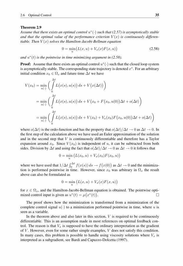
2.6 Optimal Control 35
Theorem 2.9Assume that there exists an optimal control u∗(·) such that (2.57) is asymptotically stableand that the optimal value of the performance criterion V (x) is continuously differen-tiable. Then V (x) solves the Hamilton-Jacobi-Bellman equation
0 = minu
(L(x, u) + Vx(x)F (x, u)
)(2.58)
and u∗(t) is the pointwise in time minimizing argument in (2.58).
Proof: Assume that there exists an optimal control u∗(·) such that the closed loop systemis asymptotically stable. The corresponding state trajectory is denoted x∗. For an arbitraryinitial condition x0 ∈ Ωx and future time ∆t we have
V (x0) = minu(·)
( ∆t∫0
L(x(s), u(s)
)ds+ V
(x(∆t)
))
= minu(·)
( ∆t∫0
L(x(s), u(s)
)ds+ V
(x0 + F
(x0, u(0)
)∆t+ o(∆t)
)
= minu(·)
( ∆t∫0
L(x(s), u(s)
)ds+ V (x0) + Vx(x0)F
(x0, u(0)
)∆t+ o(∆t)
)where o(∆t) is the ordo-function and has the property that o(∆t)/∆t→ 0 as ∆t→ 0. Inthe first step of the calculation above we have used an Euler approximation of the solutionand in the second step that V is continuously differentiable and therefore has a Taylorexpansion around x0. Since V (x0) is independent of u, it can be subtracted from bothsides. Division by ∆t and using the fact that o(∆t)/∆t→ 0 as ∆t→ 0 it follows that
0 = minu
(L(x0, u) + Vx(x0)F (x0, u)
)where we have used that 1/∆t
∫∆t
0f(x(s)) ds→ f
(x(0)
)as ∆t→ 0 and the minimiza-
tion is performed pointwise in time. However, since x0 was arbitrary in Ωx the resultabove can also be formulated as
0 = minu
(L(x, u) + Vx(x)F (x, u)
)for x ∈ Ωx, and the Hamilton-Jacobi-Bellman equation is obtained. The pointwise opti-mized control input is given as u∗(t) = µ
(x∗(t)
).
The proof shows how the minimization is transformed from a minimization of thecomplete control signal u(·) to a minimization performed pointwise in time, where u isseen as a variable.
In the theorem above and also later in this section, V is required to be continuouslydifferentiable. This is an assumption made in most references on optimal feedback con-trol. The reason is that Vx is supposed to have the ordinary interpretation as the gradientof V . However, even for some rather simple examples, V does not satisfy this condition.In many cases, this problem is possible to handle using viscosity solutions where Vx isinterpreted as a subgradient, see Bardi and Capuzzo-Dolcetta (1997).
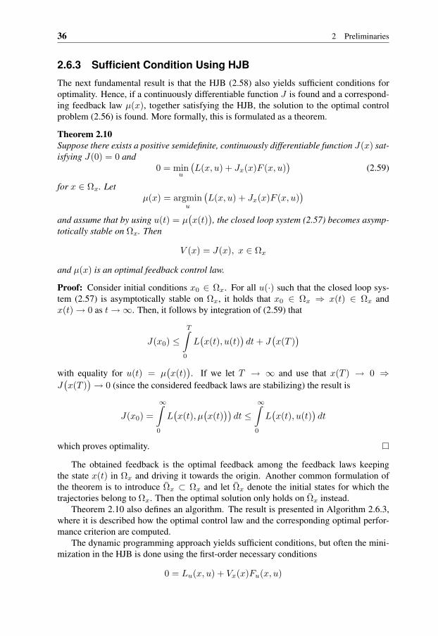
36 2 Preliminaries
2.6.3 Sufficient Condition Using HJB
The next fundamental result is that the HJB (2.58) also yields sufficient conditions foroptimality. Hence, if a continuously differentiable function J is found and a correspond-ing feedback law µ(x), together satisfying the HJB, the solution to the optimal controlproblem (2.56) is found. More formally, this is formulated as a theorem.
Theorem 2.10Suppose there exists a positive semidefinite, continuously differentiable function J(x) sat-isfying J(0) = 0 and
0 = minu
(L(x, u) + Jx(x)F (x, u)
)(2.59)
for x ∈ Ωx. Letµ(x) = argmin
u
(L(x, u) + Jx(x)F (x, u)
)and assume that by using u(t) = µ
(x(t)
), the closed loop system (2.57) becomes asymp-
totically stable on Ωx. Then
V (x) = J(x), x ∈ Ωx
and µ(x) is an optimal feedback control law.
Proof: Consider initial conditions x0 ∈ Ωx. For all u(·) such that the closed loop sys-tem (2.57) is asymptotically stable on Ωx, it holds that x0 ∈ Ωx ⇒ x(t) ∈ Ωx andx(t) → 0 as t→∞. Then, it follows by integration of (2.59) that
J(x0) ≤T∫
0
L(x(t), u(t)
)dt+ J
(x(T )
)with equality for u(t) = µ
(x(t)
). If we let T → ∞ and use that x(T ) → 0 ⇒
J(x(T )
)→ 0 (since the considered feedback laws are stabilizing) the result is
J(x0) =
∞∫0
L(x(t), µ
(x(t)
))dt ≤
∞∫0
L(x(t), u(t)
)dt
which proves optimality.
The obtained feedback is the optimal feedback among the feedback laws keepingthe state x(t) in Ωx and driving it towards the origin. Another common formulation ofthe theorem is to introduce Ωx ⊂ Ωx and let Ωx denote the initial states for which thetrajectories belong to Ωx. Then the optimal solution only holds on Ωx instead.
Theorem 2.10 also defines an algorithm. The result is presented in Algorithm 2.6.3,where it is described how the optimal control law and the corresponding optimal perfor-mance criterion are computed.
The dynamic programming approach yields sufficient conditions, but often the mini-mization in the HJB is done using the first-order necessary conditions
0 = Lu(x, u) + Vx(x)Fu(x, u)
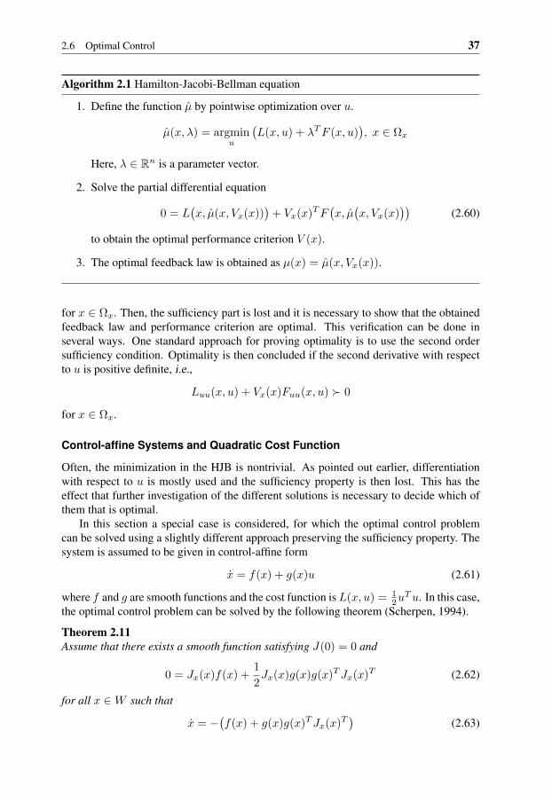
2.6 Optimal Control 37
Algorithm 2.1 Hamilton-Jacobi-Bellman equation
1. Define the function µ by pointwise optimization over u.
µ(x, λ) = argminu
(L(x, u) + λTF (x, u)
), x ∈ Ωx
Here, λ ∈ Rn is a parameter vector.
2. Solve the partial differential equation
0 = L(x, µ(x, Vx(x))
)+ Vx(x)TF
(x, µ
(x, Vx(x)
))(2.60)
to obtain the optimal performance criterion V (x).
3. The optimal feedback law is obtained as µ(x) = µ(x, Vx(x)).
for x ∈ Ωx. Then, the sufficiency part is lost and it is necessary to show that the obtainedfeedback law and performance criterion are optimal. This verification can be done inseveral ways. One standard approach for proving optimality is to use the second ordersufficiency condition. Optimality is then concluded if the second derivative with respectto u is positive definite, i.e.,
Luu(x, u) + Vx(x)Fuu(x, u) 0
for x ∈ Ωx.
Control-affine Systems and Quadratic Cost Function
Often, the minimization in the HJB is nontrivial. As pointed out earlier, differentiationwith respect to u is mostly used and the sufficiency property is then lost. This has theeffect that further investigation of the different solutions is necessary to decide which ofthem that is optimal.
In this section a special case is considered, for which the optimal control problemcan be solved using a slightly different approach preserving the sufficiency property. Thesystem is assumed to be given in control-affine form
x = f(x) + g(x)u (2.61)
where f and g are smooth functions and the cost function isL(x, u) = 12u
Tu. In this case,the optimal control problem can be solved by the following theorem (Scherpen, 1994).
Theorem 2.11Assume that there exists a smooth function satisfying J(0) = 0 and
0 = Jx(x)f(x) +12Jx(x)g(x)g(x)TJx(x)T (2.62)
for all x ∈W such that
x = −(f(x) + g(x)g(x)TJx(x)T
)(2.63)

38 2 Preliminaries
is asymptotically stable on Ωx ⊂W . Then, V (x) is the solution to (2.62) such that (2.63)is asymptotically stable for all x ∈ Ωx.
Proof: Assume that (2.62) has a smooth solution J(x) on Ωx. Then for all u(·) such thatthe solution to the closed loop system satisfies x(t) ∈ Ωx for all t ≤ 0 and x(t) → 0 ast→ −∞, we have
J(x(0)
)=
0∫−∞
d
dtJ(x) dt =
0∫−∞
12Jx
(x)g(x)g(x)TJx(x)T dt
=12
0∫−∞
‖u‖2 dt− 12
0∫−∞
‖u− g(x)TJx(x)T ‖2 dt ≤ 12
0∫−∞
‖u‖2 dt
for all x(0) ∈ Ωx and hence J(x) is a lower bound for 12
∫ 0
−∞ ‖u‖2 dt. It is also clearthat this bound is obtained by using the feedback law u(x) = g(x)TJx(x)T . By theasymptotic stability of (2.63) on Ωx, the latter feedback law is such that x(t) → 0 ast→ −∞ and the optimal performance criterion V (x) is therefore found as
V (x) = J(x), x ∈ Ωx
The proof is illustrative, because it shows how an optimal control problem for a state-space system can be solved if the system is affine in the control input and has a quadraticcost function. We will use similar reasoning in Section 5.3 to compute the controllabilityfunction for descriptor systems.
2.6.4 Example
A small, but yet illustrative, example is presented below. It shows how Algorithm 2.6.3can be used and some different behaviors that may occur. Consider the system
x = αx+ u (2.64)
where x and α both belong to R. The objective is to find a stabilizing feedback law suchthat
J =12
∞∫0
βx4 + u2 dt (2.65)
is minimized, where β ∈ R. We are interested in a global feedback law and thereforeΩx = R. For notational convenience we define
H(x, u, λ) =12βx4 +
12u2 + λ(αx+ u)
where λ ∈ R. The HJB for the given problem can be formulated as
0 = minuH(x, u, λ)
2.6 Optimal Control 39
The first order necessary condition for optimality, i.e., Hu(x, u, λ) = 0, yields the feed-back law
µ(x, λ) = −λand the second order sufficient condition becomes Huu(x, u, λ) = 1/2 > 0 for allx. Hence, the obtained feedback law must be optimal if u = µ(x) = µ
(x, Vx(x)
)makes (2.64) asymptotically stable. The partial differential equation in part 2 of Algo-rithm 2.6.3 becomes
0 = Vx(x)2 − 2αx− βx4
which has the solutionsVx(x) = αx± |x|
√α2 + βx2
The optimal feedback law then has the form
u = −αx∓ |x|√α2 + βx2
and the corresponding closed loop system is
x = ∓|x|√α2 + βx2
Since an asymptotically stable closed loop system is desired, the optimal feedback lawand Vx(x) can be written as
u = −(α+
√α2 + βx2
)x, Vx(x) =
(α+
√α2 + βx2
)x (2.66)
and by integration of Vx(x), the optimal cost is obtained as
V (x) =12αx2 +
13β(α2 + βx2
) 32 − 1
3β(α2)
32 (2.67)
since V (0) = 0. Using the parameters α and β, the behavior of the optimal controlproblem can be changed. To get a well-posed problem, β ≥ 0 is assumed. Three differentcases will be investigated:
1. β > 0, α arbitrary:In this case the state is included in the cost function and (2.64) is either asymptoti-cally stable, a pure integrator or unstable depending of the choice of α. For β > 0it follows that
α+√α2 + βx2 > 0
for all x 6= 0, but if x = 0 the system is at the equilibrium. If (2.67) is studied, itcan be seen that a small β yields a small cost and vice versa. Furthermore, it can berealized that if α < 0, i.e., the undriven system is asymptotically stable, a smallercost is obtained than if α > 0. These observations coincide with the intuition, sincein first case the undriven system helps the feedback law to reach the origin.
2. β = 0, α > 0:In this case, the state is not included in the performance criterion and the system isunstable. The expressions in (2.66) will in this case be
u = −(α+
√α2)x = −2αx, Vx(x) =
(α+
√α2)x = 2αx
40 2 Preliminaries
and the cost function isV (x) = αx2
If α is large, i.e., if the divergence is fast, a larger performance criterion is obtainedwhich corresponds to the intuition. Note the comments in the beginning of thissection about x being present in L. It is possible to choose Vx(x) = 0 and satisfythe HJB. However, the closed loop system is then unstable, and it is necessary toexplicitly choose the stabilizing control law.
3. β = 0, α < 0:In this case, the state is not included in the cost function and the system is asymp-totically stable. The expressions corresponding to (2.66) becomes
u = −(α+
√α2)x = 0, Vx(x) =
(α+
√α2)x = 0
and a optimal performance criterion V (x) = 0. This is natural, since it does notcost anything to have a nonzero state and the state goes towards the origin withoutusing the control signal. Of course, it is cheapest not to use the control signal inthis case.
3Optimal Feedback Control for
Descriptor Systems
In principle, the problem of finding optimal feedback laws for descriptor systems can besolved by the theory for state-space systems. The reason is that given certain regularityconditions we know from Section 2.4 that a rather general class of descriptor system canbe reduced to either a reduced size state-space system and some algebraic equations or toa state-space system together with conditions on the initial conditions. In both cases, theobtained system can be handled by the theory presented in Section 2.6.
A problem is that it is often not possible to compute the underlying state-space systemexplicitly because no explicit inverse exists. Therefore, it is interesting to find methods tocompute the optimal feedback law either based on a general descriptor system or at leastbased on an index reduced description.
As far as as we know, no approach exists such that a general descriptor system (2.2)can be treated immediately without index reduction. However, for linear time-invariantdescriptor systems (2.5) such methods exist, see for example (Bender and Laub, 1987;Mehrmann, 1989). These methods are based on variational calculus which leads to ageneralized eigenvalue problem to be solved, see Jonckheere (1988). For nonlinear de-scriptor systems in semi-explicit form (2.4), there are also results based on the dynamicprogramming approach. In Xu and Mizukami (1993) an equation similar to the HJB isderived. We will in this chapter present this HJB-like equation and investigate how its so-lution is related to the solution of the corresponding HJB for a reduced state-space modeldescribing the same system.
The chapter is organized as follows. The optimal feedback control problem is for-mulated in Section 3.1. In Section 3.2, the descriptor system is rewritten as a state-spacesystem and the optimal control problem is solved using the ordinary HJB equation. InSection 3.3, the HJB-like equation is used instead to find the optimal solution and Sec-tion 3.4 shows how the different methods relate to each other. A special case, for whichthe first order conditions for optimality become simple, is described in Section 3.5. Fi-nally, a small example is presenter in Section 3.6.
41
42 3 Optimal Feedback Control for Descriptor Systems
3.1 Optimal Feedback Control
Consider a semi-explicit system description
x1 = F1(x1, x2, u) (3.1a)0 = F2(x1, x2, u) (3.1b)
which is assumed to satisfy Assumption A2 for x1 ∈ Ωx and the corresponding set for(x1, x2, u) is denoted Ω. The system description (3.1) can be the result of the indexreduction method in Section 2.4.3 in a case when Assumption A3 is satisfied.
The considered class of performance criterions is
J =
∞∫0
L(x1, x2, u) dt (3.2)
with an infinite time horizon and with a cost function L that is positive semidefinite andpositive definite in u. The optimal control problem can then be formulated as
V(x1(0)
)= min
u(·)J (3.3)
subject to the dynamics (3.1) and the boundary conditions
x1(0) = x1,0 ∈ Ωx
limt→∞
x1(t) = 0
The minimization is done with respect to all u(·) such that two conditions are satisfied.One condition is that the obtained closed loop system
x1 = F1
(x1, x2, u(·)
)(3.4a)
0 = F2
(x1, x2, u(·)
)(3.4b)
is asymptotically stable, see Section 2.5. Another condition, specific for the descriptorsystem case, is that (3.4) is required to have index one. This condition is added sincedifferent feedback laws u = k(x1, x2) may yield different indices of (3.4). The effectwould be that the size of dynamical and algebraical part would change and that someof the variables x1 could be algebraically determined by the other variables in x1 andx2. It would also make the problem harder to analyze, since implicit constraints couldoccur. However, in the case when the system is given in semi-explicit form satisfyingAssumption A2 it will be shown that the index is automatically preserved for the optimalcontrol input u(·). Therefore since the closed loop system (3.4) has index one, it is knownthat x1 defines the dynamical part and x2 is algebraically connected to x1. The initialconditions are then given for x1 while the initial conditions for x2 are assumed to bechosen consistently, i.e., such that F2
(x1,0, x2,0, u(x1,0)
)= 0. Assumption A2 together
with the fact that only consistent initial conditions are considered also yields that theclosed loop system will have a unique solution. This is an important fact when it comesto V being a function of the initial conditions only.
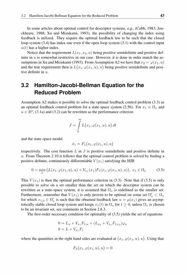
3.2 Hamilton-Jacobi-Bellman Equation for the Reduced Problem 43
In some articles about optimal control for descriptor systems, e.g., (Cobb, 1983; Jon-ckheere, 1988; Xu and Mizukami, 1993), the possibility of changing the index usingfeedback is utilized. They require the optimal feedback law to be such that the closedloop system (3.4) has index one even if the open loop system (3.1) with the control inputu(t) has a higher index.
Notice that the requirement L(x1, x2, u) being positive semidefinite and positive def-inite in u is somewhat restrictive in our case. However, it is done in order match the as-sumptions in Xu and Mizukami (1993). From Assumption A2 we have that x2 = ϕ(x1, u)and the true requirement then is L
(x1, ϕ(x1, u), u
)being positive semidefinite and posi-
tive definite in u.
3.2 Hamilton-Jacobi-Bellman Equation for theReduced Problem
Assumption A2 makes it possible to solve the optimal feedback control problem (3.3) asan optimal feedback control problem for a state-space system (2.56). For x1 ∈ Ωx andu ∈ Rp, (3.1a) and (3.2) can be rewritten as the performance criterion
J =
∞∫0
L(x1, ϕ(x1, u), u
)dt
and the state-space modelx1 = F1
(x1, ϕ(x1, u), u
)respectively. The cost function L in J is positive semidefinite and positive definite inu. From Theorem 2.10 it follows that the optimal control problem is solved by finding apositive definite, continuously differentiable V (x1) satisfying the HJB
0 = minu
(L(x1, ϕ(x1, u), u) + Vx1(x1)F1(x1, ϕ(x1, u), u)
), x1 ∈ Ωx (3.5)
This V (x1) is then the optimal performance criterion in (3.3). Note that if (3.5) is onlypossible to solve on a set smaller than the set on which the descriptor system can berewritten as a state-space system, it is assumed that Ωx is redefined as the smaller set.Furthermore, remember that V (x1) is only proven to be optimal on some set Ω′
x ⊂ Ωx
for which x1,0 ∈ Ω′x is such that the obtained feedback law u = µ(x1) gives an asymp-
totically stable closed loop system and keeps x1(t) in Ωx for t ≥ 0, unless Ωx is chosento be an invariant set, see comments in Section 2.6.3.
The first-order necessary condition for optimality of (3.5) yields the set of equations
0 = Lu + Vx1F1;u + (Lx2 + Vx1F1;x2)ϕu
0 = L+ Vx1F1
where the quantities in the right hand sides are evaluated at(x1, ϕ(x1, u), u
). Using that
F2
(x1, ϕ(x1, u), u
)= 0

44 3 Optimal Feedback Control for Descriptor Systems
identically in u, differentiation with respect to u gives
F2,x2
(x1, ϕ(x1, u), u
)ϕu(x1, u) + F2,u
(x1, ϕ(x1, u), u
)= 0
which can be solved for ϕu(x1, u) as
ϕu(x1, u) = −F2,x2
(x1, ϕ(x1, u), u
)−1F2,u
(x1, ϕ(x1, u), u
)Since x2 = ϕ(x1, u) is the unique solution of (3.1b), it is also possible to write theseequations according to
0 = Lu + Vx1F1;u − (Lx2 + Vx1F1;x2)F−12,x2
F2;u (3.7a)
0 = L+ Vx1F1 (3.7b)0 = F2 (3.7c)
where the right hand sides are evaluated at x1, x2, u. One way of looking at (3.7) is toregard (3.7a) and (3.7c) as p + n2 equations from which one tries to solve for u and x2
as functions of x1 and Vx1 . When these quantities are substituted into (3.7b) the resultis a first order partial differential equation for V as a function of x1. When this partialdifferential equation is solved the result can be substituted back into the expression for uto give the optimal feedback law.
To ensure that the optimal solution is found, the second order sufficient conditionmentioned in Section 2.6.3 can be used. It will require ϕuu to be computed which ispossible but the expressions become rather involved.
3.3 Hamilton-Jacobi-Bellman-Like Equation
In Xu and Mizukami (1993) the optimal control problem (3.3) is solved in a differentmanner. According to their Theorem 3.1 it is possible to find the optimal solution bysolving the Hamilton-Jacobi-Bellman-like equation
0 = minu
(L(x1, x2, u) +W1(x1)F1(x1, x2, u) +W2(x1, x2)F2(x1, x2, u)
)(3.8)
for some continuous functions W1(x1) and W2(x1, x2) such that W1(x1) is a gradient ofsome continuously differentiable function V (x1). This V (x1) is then the optimal cost in(3.3).
Using the first-order necessary condition for optimality, the control is defined by thefollowing set of equations
0 = Lu(x1, x2, u) +W1(x1)F1;u(x1, x2, u) +W2(x1, x2)F2;u(x1, x2, u) (3.9a)0 = L(x1, x2, u) +W1(x1)F1(x1, x2, u) +W2(x1, x2)F2(x1, x2, u) (3.9b)
where x2 is considered to be independent of u when differentiating with respect to u.From these equations it is not immediately obvious how to obtain a relation from whichW1 can be computed. Similar equations to (3.7) can be obtained by restricting (3.9) to

3.4 Relationships Among the Solutions 45
points satisfying F2 = 0. Then the result is the following system
0 = Lu(x1, x2, u) +W1(x1)F1;u(x1, x2, u) +W2(x1, x2)F2;u(x1, x2, u) (3.10a)0 = L(x1, x2, u) +W1(x1)F1(x1, x2, u) (3.10b)0 = F2(x1, x2, u) (3.10c)
If W2 is considered unknown (3.10) is still underdetermined. Hence more equations areneeded orW2 is to be considered as given. However, Xu and Mizukami (1993) only givessufficient conditions, i.e., if a W1 and W2 can be found such that (3.8) is satisfied, theoptimal solution is found, and they do not mention what kind of conditions that W2 haveto satisfy. This will be investigated in the next section.
3.4 Relationships Among the Solutions
The reduced Hamilton-Jacobi equation (3.5) and the Hamilton-Jacobi-like equation (3.8)solve the same underlying optimal control problem. Therefore it is natural that the func-tions V , W1 and W2 are related and below these relationships are investigated.
Lemma 3.1Suppose there exist a function V (x1) and a feedback u = k(x1) solving (3.5) on Ωx.Then W1(x1) = Vx1(x1), u = k(x1) solve (3.8) under the constraint F2(x1, x2, u) = 0.Moreover, with the choice
W1 = Vx1 , W2 = −(Lx2 + Vx1F1;x2
)F−1
2;x2(3.11)
the necessary conditions for optimality (3.10) are satisfied for u = k(x1) together withx2 = ϕ
(x1, k(x1)
).
Proof: When F2 = 0 the right hand sides of (3.8) and (3.5) coincide. Comparing (3.7)and (3.10) shows that (3.10) is satisfied for u = k(x1), x2 = ϕ
(x1, k(x1)
).
The converse relation is given by the following lemma.
Lemma 3.2Assume that for x1 ∈ Ωx
1 it holds that:
• (3.8) has a solution u = ψ(x1, x2)
• F2
(x1, x2, ψ(x1, x2)
)= 0 has a solution x2 = η(x1)
• W1(x1) = Vx1(x1) for some function V (x1)
Then Vx1(x1) and u = k(x1) = ψ(x1, η(x1)
)solve (3.5) for x1 ∈ Ωx. Moreover, for
(x1, x2, u) ∈ Ω satisfying (3.10) it follows that
W2 = −(Lx2 +W1F1;x2
)F−1
2;x2(3.12)
1If this Ωx is smaller than the Ωx on which the system can be written as a state-space system, Ωx is redefinedas the smaller region.
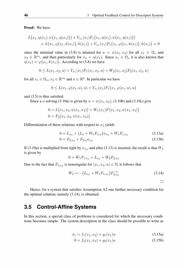
46 3 Optimal Feedback Control for Descriptor Systems
Proof: We have
L(x1, η(x1), ψ
(x1, η(x1)
))+ Vx1(x1)F1
(x1, η(x1), ψ
(x1, η(x1)
))= L
(x1, ϕ
(x1, k(x1)
), k(x1)
)+ Vx1(x1)F1
(x1, ϕ
(x1, k(x1)
), k(x1)
)= 0
since the minimal value in (3.8) is attained for u = ψ(x1, x2) for all x1 ∈ Ωx andx2 ∈ Rn2 , and then particularly for x2 = η(x1). Since x1 ∈ Ωx it is also known thatη(x1) = ϕ
(x1, k(x1)
). According to (3.8) we have
0 ≤ L(x1, x2, u) + Vx1(x1)F1(x1, x2, u) +W2(x1, x2)F2(x1, x2, u)
for all x1 ∈ Ωx, x2 ∈ Rn2 and u ∈ Rp. In particular we have
0 ≤ L(x1, ϕ(x1, u), u) + Vx1(x1)F1
(x1, ϕ(x1, u), u
)and (3.5) is thus satisfied.
Since a u solving (3.10a) is given by u = ψ(x1, x2), (3.10b) and (3.10c) give
0 = L(x1, x2, ψ(x1, x2)
)+W1(x1)F
(x1, x2, ψ(x1, x2)
)0 = F2
(x1, x2, ψ(x1, x2)
)Differentiation of these relations with respect to x2 yields
0 = Lx2 +(Lu +W1F1;u
)ψx2 +W1F1;x2 (3.13a)
0 = F2;x2 + F2;uψx2 (3.13b)
If (3.10a) is multiplied from right by ψx2 and after (3.13) is inserted, the result is that W2
is given by0 = W1F1;x2 + Lx2 +W2F2;x2
Due to the fact that F2;x2 is nonsingular for (x1, x2, u) ∈ Ω, it follows that
W2 = −(Lx2 +W1F1;x2
)F−1
2;x2(3.14)
Hence, for a system that satisfies Assumption A2 one further necessary condition forthe optimal solution, namely (3.14), is obtained.
3.5 Control-Affine Systems
In this section, a special class of problems is considered for which the necessary condi-tions becomes simple. The system description in the class should be possible to write as
x1 = f1(x1, x2) + g1(x1)u (3.15a)0 = f2(x1, x2) + g2(x1)u (3.15b)

3.6 Example 47
while the cost function should be expressed in the form L(x1, x2, u) = l(x1) + 12u
Tu.Then (3.10a) can be solved explicitly in u for all x1, x2 since (3.10a) will become
0 = uT −W1(x1)g1(x1)−W2(x1, x2)g2(x1) (3.16)
and from Lemma 3.2, we have
W2(x1, x2) = −W1(x1)f1;x2(x1, x2)f−12;x2
(x1, x2) (3.17)
Note that f2,x2(x1, x2) is nonsingular for all (x1, x2) such that f2(x1, x2) = 0 is solvablesince F2,x2(x1, x2, u) is nonsingular for all (x1, x2, u) ∈ Ω and then particularly foru = 0. Combining (3.16) and (3.17) yields
u = −g(x1, x2)TW1(x1)T
and after some manipulation the necessary conditions can be rewritten as
0 = l(x1) +W1(x1)f(x1, x2)−12W1(x1)g(x1, x2)g(x1, x2)TW1(x1)T (3.18a)
0 = f2(x1, x2) + g2(x1)g(x1, x2)TW1(x1)T (3.18b)
where
f(x1, x2) = f1(x1, x2)− f1;x2(x1, x2)f−12;x2
(x1, x2)f2(x1, x2)
g(x1, x2) = g1(x1)− f1;x2(x1, x2)f−12;x2
(x1, x2)g2(x1)
3.6 Example
In this section a small example showing the different methods is presented.Consider the simple system
x1 = x2
0 = u− x31 − x2
which satisfies Assumption A2 with performance criterion
J =
∞∫0
(x21
2+u2
2)dt
The necessary conditions (3.7) give
0 = u+ Vx1 · 0 + Vx1 · 1
0 =x2
1
2+u2
2+ Vx1x2
0 = u− x31 − x2
Eliminating u and x2 gives the following equation for Vx1
V 2x1
+ 2x31Vx1 − x2
1 = 0

48 3 Optimal Feedback Control for Descriptor Systems
To get a positive definite solution for V the solution for Vx1 must be chosen as
Vx1 = x1(√
1 + x41 − x2
1)
and the corresponding optimal feedback law then becomes
u = −Vx1 = −x1(√
1 + x41 − x2
1)
If the problem is instead solved using (3.9) we get the equations
0 = u+W1 · 0 +W2 · 1
0 =x2
1
2+u2
2+W1x2 +W2(u− x3
1 − x2)
Since the system satisfies Assumption A2, it is known from Lemma 3.2 that W2 mustsatisfy (3.14), i.e.,
W2 = W1
When the equation 0 = u − x31 − x2 is satisfied this gives the same equation for W1 as
for Vx1 so the solution is the same.
4Power Series Solution of the
Hamilton-Jacobi-Bellman Equation
In Chapter 3 we discussed optimal control for descriptor systems on semi-explicit form,which possibly could come from higher index problems. Unfortunately, there are practi-cal issues with the methods presented there. One issue is that in order to explicitly and notnumerically, solve the optimality conditions an explicit expression for the implicit func-tion ϕ is needed. However, in many cases the implicit function is not possible to expresson closed form. Another problem with the methods in Chapter 3 is that even if ϕ can beexpressed explicitly, it is only for a small class of problems the optimality conditions canbe solved to obtain an explicit solution. Therefore, another approach to solve the optimalcontrol problem will be presented in this chapter.
The idea is to instead compute the optimal solution, i.e., the optimal performancecriterion and the corresponding feedback law, expressed as power series expansions. Forstate-space models this idea was first considered by Al’brekht (1961). He shows that theterms in the power series expansions can be sequentially obtained through solution of aquadratic optimal control problem for the linearized system and subsequent solution of aseries of linear partial differential equations. Further, a formal proof of the convergence ofthe power series is presented in the case when the input signal is scalar and the system hasthe form x = f(x)+Bu. In Lee and Markus (1967) these results are extended to generalstate-space systems, x = f(x, u), and this work is extended even more in Lukes (1969).In the earlier works (Al’brekht, 1961; Lee and Markus, 1967), the functions involved arerequired to be analytic functions around the origin. In Lukes (1969), this requirementis relaxed to twice differentiability. An alternative proof to the one presented in Lukes(1969) is given in van der Schaft (1991) where the requirements on the cost function arerelaxed. Krener (1992) studied the case when the dynamics of an external signal generatorare included and in Krener (2001) he also investigated the case when the system is notstabilizable or not detectable. The latter reference also considers the Hamilton-Jacobiinequality.
Other classes of problems also studied are for example the case with bilinear system
49
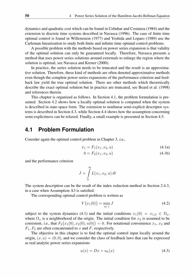
50 4 Power Series Solution of the Hamilton-Jacobi-Bellman Equation
dynamics and quadratic cost which can be found in Cebuhar and Costanza (1984) and theextension to discrete time systems described in Navasca (1996). The case of finite timeoptimal control is found in Willemstein (1977) and Yoshida and Loparo (1989) use theCarleman linearization to study both finite and infinite time optimal control problems.
A possible problem with the methods based on power series expansion is that validityof the optimal solution can only be guaranteed locally. Therefore, Navasca presents amethod that uses power series solutions around extremals to enlarge the region where thesolution is optimal, see Navasca and Krener (2000).
In practice, the series solution needs to be truncated and the result is an approxima-tive solution. Therefore, these kind of methods are often denoted approximative methodseven though the complete power series expansions of the performance criterion and feed-back law yield the true optimal solution. There are other methods which theoreticallydescribe the exact optimal solution but in practice are truncated, see Beard et al. (1998)and references therein.
This chapter is organized as follows. In Section 4.1, the problem formulation is pre-sented. Section 4.2 shows how a locally optimal solution is computed when the systemis described in state-space form. The extension to nonlinear semi-explicit descriptor sys-tems is described in Section 4.3, while Section 4.4 shows how the assumption concerningsemi-explicitness can be relaxed. Finally, a small example is presented in Section 4.5.
4.1 Problem Formulation
Consider again the optimal control problem in Chapter 3, i.e.,
x1 = F1(x1, x2, u) (4.1a)0 = F2(x1, x2, u) (4.1b)
and the performance criterion
J =
∞∫0
L(x1, x2, u) dt
The system description can be the result of the index reduction method in Section 2.4.3,in a case when Assumption A3 is satisfied.
The corresponding optimal control problem is written as
V(x1(0)
)= min
u(·)J (4.2)
subject to the system dynamics (4.1) and the initial conditions x1(0) = x1,0 ∈ Ωx,where Ωx is a neighborhood of the origin. The initial condition for x2 is assumed to beconsistent, i.e., that F2
(x1(0), x2(0), u(0)
)= 0. For notational convenience x1, x2 and
F1, F2 are often concatenated to x and F , respectively.The objective in this chapter is to find the optimal control input locally around the
origin, (x, u) = (0, 0), and we consider the class of feedback laws that can be expressedas real analytic power series expansions
u(x) = Dx+ uh(x) (4.3)

4.2 Review of the State-Space System Case 51
where uh(x) consists of terms of at least degree two.Mostly in this thesis it is assumed that the system satisfies Assumption A2, but in this
case a more convenient assumption is as follows.
Assumption A4. It holds that F2(0, 0, 0) = 0 and that F2;x2(0, 0, 0) is nonsingular.
Assumption A4 together with Theorem A.1 yield existence of a neighborhood Ωx1,u
of the origin such that for (x1, u) ∈ Ωx1,u
x2 = ϕ(x1, u)
Furthermore, we assume that the system has an equilibrium at the origin, which alsoyields that ϕ(0, 0) = 0. We also make an assumption regarding the system functions.
Assumption A5. The functions F (x, u) and L(x, u) are real analytic functions in someopen set
W = (x1, u) ∈ Wx1,u, x2 ∈ Wx2 ⊃ ϕ(Wx1,u) (4.4)
where Wx1,u and Wx2 are neighborhoods of (x1, u) = 0 and x2 = 0, respectively.
Note that since Wx2 is a neighborhood it is open, which not ϕ(Wx1,u) necessarily isdespite the fact that Wx1,u is a neighborhood and therefore is open.
The analyticity of F and L yields that they can be expanded in convergent powerseries
F (x, u) = Ax+Bu+ Fh(x, u) (4.5a)
L(x, u) = xTQx+ 2xTSu+ uTRu+ Lh(x, u) (4.5b)
where the matrices A, B, Q and S are partitioned as
A =(A11 A12
A21 A22
), B =
(B1
B2
), Q =
(Q11 Q12
Q21 Q22
), S =
(S1
S2
)and Fh(x, u) and Lh(x, u) contain higher order terms of at least degree two and three,respectively. The matrix A22 will be nonsingular since it was assumed in Assumption A4that F2;x2(0, 0, 0) = A22 is nonsingular.
In the computations it will be assumed that the analysis is done in a neighborhoodwhere both Assumption A4 and Assumption A5 are satisfied. To lessen the notationalcomplexity, Ωx1,u is assumed to be covered by Wx1,u, i.e., Ωx1,u ⊂ Wx1,u.
As mentioned in Section 3.1 the optimization is done with respect to control inputssuch that the closed loop system is asymptotically stable and has index one locally aroundthe origin. Under the assumption that the initial conditions are chosen close enough to theorigin, it is known from Theorem 2.5, i.e., Lyapunov’s indirect method, that a sufficientcondition is asymptotic stability of the linearization of the closed loop system.
4.2 Review of the State-Space System Case
First a short review is presented describing how to obtain a power series solution to anoptimal control problem in the case when the system is described by a state-space model.

52 4 Power Series Solution of the Hamilton-Jacobi-Bellman Equation
In the state-space case it is known from Section 2.6 that the optimal control problemmentioned in Section 4.1 is associated with the HJB equation
0 = minu(·)
L(x, u) + Vx(x)F (x, u) (4.6)
which corresponds to first-order necessary conditions for optimality
0 = L(x, u∗(x)
)+ Vx(x)F
(x, u∗(x)
)0 = Lu
(x, u∗(x)
)+ Vx(x)Fu
(x, u∗(x)
) (4.7)
for the optimal performance criterion V (x) and the optimal feedback law u∗(x).The idea is that if L(x, u), F (x, u) and u(x) are real analytical near the origin and if
u(x) is chosen such that it stabilizes the closed loop system locally around (x, u) = 0, theperformance criterion V (x) will be analytical in a neighborhood of the origin, see Lukes(1969). This guarantees that V (x) can be expressed as a convergent power series
V (x) = xTPx+ Vh(x) (4.8)
where Vh(x) contains the terms of order three and higher. Lukes (1969) also shows thatP is a positive definite matrix if only cost matrices satisfying(
Q SST R
) 0 (4.9)
is considered. Positive definiteness of P will be important when determining which ofthe solutions to the necessary conditions (4.7) is optimal.
If (4.3), (4.5) and (4.8) are inserted into (4.7), the result is two polynomial equationsin x. These polynomial equations are supposed to hold for all x in a neighborhood of theorigin and different orders of xwill then yield separate equations in the corresponding co-efficients. According to Lukes (1969), the lowest order terms of the polynomial equationsyield the equations
PA+ ATP − PBR−1BTP +Q− SR−1ST = 0 (4.10a)
D∗ +R−1(ST +BTP
)= 0 (4.10b)
where A = A−BR−1ST , while the higher order terms in x will be
V [m]x (x)Acx = −
m−1∑k=3
V [k]x (x)Bu[m−k+1]
∗ (x)
−m−1∑k=2
V [k]x (x)F [m−k+1]
h (x, u∗)− L[m]h (x, u∗)
− 2bm−1
2 c∑k=2
u[k]∗ (x)TRu
[m−k]∗ (x)− u
[m/2]∗ (x)TRu
[m/2]∗ (x)
(4.11a)
where m = 3, 4, . . . and Ac = A+BD∗, and
u[k]∗ (x) = −1
2R−1
(V [k+1]
x (x)B+k−1∑i=1
V [k−i+1]x (x)F [i]
h;u(x, u∗)+L[k]h;u(x, u∗)
)(4.11b)
4.2 Review of the State-Space System Case 53
for k = 2, 3, . . .. In the equations above, f [i] denotes the ith order terms of f and bic de-notes the floor function, which gives the largest integer less than or equal to i. Moreover,in (4.11) we use the conventions that
∑lk = 0 for l < k and that the terms u[m/2] are to
be omitted if m is odd.The equations (4.10) and (4.11) are only necessary conditions for optimality and if
several solutions exist it is necessary to decide which is optimal. The second order suf-ficient condition, i.e., Luu(x, u) + Vx(x)Fuu(x, u), evaluated in (x, u) = 0 is positivedefinite because R 0. Therefore, it is known that locally in some neighborhood of x,the necessary conditions also yield the optimal solution. However, the optimal solutionmust also satisfy the requirements in the problem formulation. That is, u∗(x) must stabi-lize the closed loop system locally around the origin and therefore Ac = A+BD∗ mustbe Hurwitz. If only cost matrices satisfying (4.9) are considered we also know that Pmust be positive definite.
The matrices P and D∗ are given by (4.10), where (4.10a) is an algebraic Riccatiequation (ARE). Hence, the ARE must have a positive definite solution P such that D∗from (4.10b) is stabilizing. A criteria for when such a solution exists is given by thefollowing lemma.
Lemma 4.1Consider the ARE (4.10a). Assume that the cost matrix satisfies
(Q S
ST R
) 0. Then the
following statements are equivalent:
1. (A,B) is stabilizable.
2. The ARE (4.10a) has a unique positive definite stabilizing solution P , i.e., a solutionsuch that A+BD∗ is Hurwitz, where D∗ is given by (4.10b).
Proof: See Lukes (1968).
Note that under the assumptions given in Lemma 4.1, the positive definite solution Pis the only positive semidefinite solution as well (Bittanti et al., 1991).
The first order terms of u∗(x) and V (x) are then unique and given by the expressions
u[1]∗ (x) = D∗x, V [2](x) = xTPx (4.12)
In order to obtain higher order approximations of the optimal feedback law u∗(x) andthe corresponding performance criterion V (x), we need to solve (4.11). First observe that
F[k]h (x, u∗) = F
[k]h (x, u[1]
∗ + u[2]∗ + . . .+ u
[k−1]∗ )
L[k]h (x, u∗) = L
[k]h (x, u[1]
∗ + u[2]∗ + . . .+ u
[k−2]∗ )
since Fh(x, u) and Lh(x, u) are power series beginning with terms of order two and three,respectively. Based on this it can be seen that the right-hand side of (4.11a) depends onlyon the terms
u[1]∗ , . . . , u
[m−2]∗ , V [2], . . . , V [m−1] (4.13)
while the right-hand side of (4.11b) depends only on
u[1]∗ , . . . , u
[k−1]∗ , V [2], . . . , V [k+1] (4.14)

54 4 Power Series Solution of the Hamilton-Jacobi-Bellman Equation
Since Ac = A + BD∗ is Hurwitz, it is shown in for example Lyapunov (1992), thatthe partial differential equation (4.11a) is uniquely solvable for a given right-hand side.Therefore, by starting with u[1]
∗ (x) = D∗x and V [2](x) = xTPx it is possible to recur-sively compute the terms
V [3](x), u[2]∗ (x), V [4](x), u[3]
∗ (x), . . .
and thereby generating power series for u∗(x) and V (x).The method shows how arbitrarily high orders of V (x) and u∗(x) can be computed.
However, in practice an important fact is that the computational complexity is exponentialin the number of variables and the desired approximation order.
4.3 Descriptor System Case
To solve the optimal control problem (4.2) we use the same technique as in Section 3.2,i.e., reduce the descriptor system to a state-space system. For (x1, u) ∈ Ωx1,u, the dy-namical part is given by
x1 = F1(x1, u) = F1
(x1, ϕ(x1, u), u
)(4.15a)
and the cost function reduces to
L(x1, u) = L(x1, ϕ(x1, u), u
)(4.15b)
The optimal control problem (4.2) is then a state-space optimal control problem whichcan be solved using the Hamilton-Jacobi-Bellman equation
0 = minu
(L(x1, u) + Vx1(x1)F1(x1, u)
)Finding power series solutions can in this case done using the method discussed in Sec-tion 4.2.
However, a problem is that in many cases it is hard or even impossible to find anexplicit expression for ϕ(x1, u). The remedy to this problem is to discover that in orderto compute the power series solutions of V (x) and u∗(x), using the method describedin Section 4.2, only the series expansions of the functions involved, i.e., F (x, u) andL(x, u), are needed. Thus, in order to determine a power series solution to the descriptorproblem only the series expansions of F (x1, u) and L(x1, u) around (x1, u) = (0, 0),have to be computed.
4.3.1 Power Series Expansion of the Reduced Problem
The idea, used in this thesis, is to utilize that the series expansions of the composite func-tions F1(x1, u) and L(x1, u) can be computed as the compositions of the series expan-sions of F1(x1, x2, u), L(x1, x2, u) and ϕ(x1, u). The composite power series expansionsare known to converge if the functions involved are analytical, see Brown and Churchill(1996). This condition is satisfied since F1(x1, x2, u), L(x1, x2, u) are assumed to be
4.3 Descriptor System Case 55
analytical in the problem formulation and ϕ(x1, u) is analytical when F2(x1, x2, u) isanalytical, according to Theorem A.1.
Before the series expansions of F (x1, u) and L(x1, u) can be calculated, we need tocalculate the series expansion of ϕ(x1, u). This can be done recursively using the powerseries expansion of F2(x1, x2, u) as shown below.
Assumex2 = ϕ(x1, u) = ϕ[1](x1, u) + ϕh(x1, u) (4.16)
where ϕh(x1, u) contains terms of degree two and higher. From (4.5) we have that theseries expansion of F2(x1, x2, u) is given by
0 = F2(x1, x2, u) = A21x1 +A22x2 +B2u+ F2h(x1, x2, u) (4.17)
If (4.16) is combined with (4.17) the expression obtained is
0 = A21x1 +A22
(ϕ[1](x1, u) + ϕh(x1, u)
)+B2u
+ F2h
(x1, ϕ
[1](x1, u) + ϕh(x1, u), u) (4.18)
Since (4.18) must hold for all (x1, u) in a neighborhood of the origin, the first order termof ϕ(x1, u) will be given by
ϕ[1](x1, u) = −A−122 A21x1 −A−1
22 B2u (4.19)
since all other terms have degrees higher than one. Furthermore, since F2h(x1, x2, u)only contains terms with at least degree two, we have that
F[m]2h
(x1, ϕ(x1, u), u
)= F
[m]2h
(x1, ϕ
[1](x1, u) + . . .+ ϕ[m−1](x1, u), u)
(4.20)
The fact that them:th order term of F2h
(x1, ϕ(x1, u)
)only depends on terms of ϕ(x1, u)
of degree m− 1 or less, makes it is possible to derive a recursive expression for a generaldegree term of ϕ(x1, u) as
ϕ[m](x1, u) = −A−122 F
[m]2h
(x1, ϕ
[1](x1, u) + . . .+ ϕ[m−1](x1, u), u)
(4.21)
using (4.18).For later convenience the first order approximation of ϕ(x1, u), i.e., (4.19), is used to
define the variable transformation x1
ϕ[1](x1, u)u
= Π(x1
u
)=
I 0−A−1
22 A21 −A−122 B2
0 I
(x1
u
)(4.22)
The variable transformation will mainly be used compute the second order term of thereduced cost function L(x1, u).
To compute the series expansion of F1(x1, u), (4.16) is inserted into (4.5a). Thesystem (4.15a) can then be written as
x1 = Ax1 + Bu+ F1h(x1, u) (4.23)

56 4 Power Series Solution of the Hamilton-Jacobi-Bellman Equation
where A = A11 −A12A−122 A21, B = B1 −A12A
−122 B2 and
F1h(x1, u) = F1h
(x1, ϕ(x1, u), u
)+A12ϕh(x1, u) (4.24)
In the same manner, the series expansion of (4.15b) is obtained as
L(x1, u) =(x1
u
)T
ΠT
(Q SST R
)Π(x1
u
)+ Lh(x1, u)
=(x1
u
)T (Q S
ST R
)(x1
u
)+ Lh(x1, u)
(4.25)
where
Lh(x1, u) = Lh(x1, ϕ(x1, u), u) + 2xT1 Q12ϕh(x1, u)
+ 2ϕ[1](x1, u)Q22ϕh(x1, u) + ϕh(x1, u)TQ22ϕh(x1, u)
+ 2uTS2ϕh(x1, u)
(4.26)
4.3.2 Application of the Results for State-Space Systems
The system description (4.23) and the description of the cost function (4.25) is now pos-sible to incorporate in the method described in Section 4.2. Using the first order terms ofthe series expansions (4.23) and (4.25), the ARE (4.10a) and the expression for the firstorder term in the feedback (4.10b) become
P˜A+ ˜
ATP − PBR−1BTP + Q− SR−1ST = 0 (4.27a)
D∗ + R−1(ST + BTP
)= 0 (4.27b)
where ˜A = A− BR−1ST .
To compute the higher order terms of V (x1) and u∗(x1) we make use of (4.11).In (4.11) the series expansion coefficients of Fh(x, u) and Lh(x, u) are replaced by thecorresponding coefficients of F1h(x1, u) and Lh(x1, u), respectively. The result is
V [m]x1
(x1)Acx1 =−m−1∑k=3
V [k]x1
(x1)Bu[m−k+1]∗ (x1)
−m−1∑k=2
V [k]x1
(x1)F[m−k+1]1h (x1, u∗)
− 2bm−1
2 c∑k=2
u[k]∗ (x1)T Ru
[m−k]∗ (x1)
− u[m/2]∗ (x1)T Ru
[m/2]∗ (x1)− L
[m]h (x1, u∗)
(4.28a)
where m = 3, 4, . . ., Ac = A+ BD∗, and the terms u[m/2] are to be omitted if m is odd.
4.3 Descriptor System Case 57
The corresponding expression for the series expansion of the feedback law is
u[k]∗ (x1) = −1
2R−1
(V [k+1]
x1(x1)B
+k−1∑i=1
V [k−i+1]x1
(x1)F[i]1h;u(x1, u∗) + L
[k]h;u(x1, u∗)
) (4.28b)
where for k = 2, 3, . . ..In (4.28a) the terms F [i]
1h(x1, u∗) and L[i]h (x1, u∗) are given by the corresponding terms
in (4.24) and (4.26) and can therefore be expressed in terms of the series expansions ofthe original functions as
F[i]1h(x1, u∗) = F
[i]1h(x1, ϕ∗, u∗) +A12ϕ
[i]h,∗ (4.29a)
and
L[i]h (x1, u∗) = L
[i]h (x1, ϕ∗, u∗) + 2xT
1 Q12ϕ[i−1]h,∗
+ 2(ϕ[1]∗ )TQ22ϕ
[i−1]h,∗ + 2
b(i−1)/2c∑k=2
(ϕ[k]h,∗)
TQ22ϕ[i−k]h,∗
+ (ϕ[i/2]h,∗ )TQ22ϕ
[i/2]h,∗ + 2
i−2∑k=1
(u[k]∗ )TS2ϕ
[i−k]h,∗
(4.29b)
where ϕ∗ = ϕ(x1, u∗) and ϕh,∗ = ϕh(x1, u∗).The series expansion coefficients of the functions F1h and Lh were obtained as (4.29a)
and (4.29b), respectively. In the expression for the optimal control signal (4.28b), thederivatives of F1(x1, u) and L(x1, u) with respect to u are also needed. These can befound as
F[i]1h;u(x1, u∗) = F
[i]1h;u
(x1, ϕ∗, u∗
)+
i∑j=1
F[j]1h;x2
(x1, ϕ∗, u∗)ϕ[i−j]u,∗ +A12ϕ
[i]h;u,∗
(4.30a)
where ϕ[i]h;u,∗ = ϕ
[i]h;u(x1, u∗), ϕ
[i]u,∗ = ϕ
[i]u (x1, u∗) and
L[k]h;u(x1, u∗) = L
[k]h;u(x1, ϕ∗, u∗) +
k∑j=2
L[j]h;x2
(x1, ϕ∗, u∗)ϕ[k−j]u,∗
+ 2xT1 Q12ϕ
[k−1]h;u,∗ + 2ϕ[1]
∗ Q22ϕ[k−1]h;u,∗ − 2BT
2 AT22Q22ϕ
[k]h,∗
+k−2∑j=1
(ϕ
[j]h;u,∗
)TQ22ϕ
[k−j]h,∗ +
k−2∑j=1
(ϕ
[k−j]h,∗
)TQ22ϕ
[j]h;u,∗
+ 2S2ϕ[k]h,∗ + 2
k−1∑j=1
u[j]∗ S2ϕ
[k−j]h;u,∗
(4.30b)
58 4 Power Series Solution of the Hamilton-Jacobi-Bellman Equation
Since F1h(x, u), ϕh(x1, u) and Lh(x, u) are power series of degree two, two and three,respectively, and
ϕ[i](x1, u∗) = ϕ(x1, u[1]∗ + u
[2]∗ + . . .+ u
[i]∗ )
we know that
F[i]1h(x1, u∗) = F
[i]1h(x1, u
[1]∗ + u
[2]∗ + . . .+ u
[i−1]∗ )
L[i]h (x1, u∗) = L
[i]h (x1, u
[1]∗ + u
[2]∗ + . . .+ u
[i−2]∗ )
and
F[i]1h;u(x1, u∗) = F
[i]1h;u(x1, u
[1]∗ + . . .+ u
[i]∗ )
L[i−1]h;u (x1, u∗) = L
[i]h;u(x1, u
[1]∗ . . .+ u
[i−1]∗ )
Hence, as for the state-space case, the right-hand side of (4.28a) depends only on thesequence (4.13), while the right-hand side of (4.28b) only depends on (4.14). So byrecursively compute the terms of the sequence
V [2](x1), u[1]∗ (x1), ϕ[1](x1, u
[1]∗ ), . . .
it is possible to generate the power series for V (x1), u∗(x1) and ϕ(x1, u∗(x1)
).
As was seen in (4.19) and (4.21), arbitrarily high orders of the series expansion ofϕ(x, u) can be computed in advance, based only on the series expansion of F2. How-ever, from a computational point of view, it can be noted from the sequence above, thatthe highest needed order of the series expansion of ϕ(x, u) is the desired order of theapproximation of u∗(x1).
We summarize the result in this section in Theorem 4.1 and an algorithm to computethe power series solution is found in Algorithm 4.1.
Theorem 4.1Consider the optimal control problem (4.2) with all assumptions in Section 4.1 satisfied.Furthermore, assume that the cost matrix
(Q S
ST R
) 0. Then, the following statements
are equivalent
1. (A, B) is stabilizable.
2. The optimal control problem has a unique local solution for x1 in a neighborhoodof the origin, and x2 chosen consistently.
Proof: Follows directly from the discussion above.
In the problem formulation we also had a requirement that the closed loop systemmust have index one. This requirement is automatically satisfied as a result of two facts.First, the optimal feedback law only depends on x1, i.e., u = k(x1). Second, fromAssumption A2 we know that F2;x2(x1, x2, u) is nonsingular for all u. Combined, thesefacts impose full rank of F2;x2
(x1, x2, u(x1)
)and the closed loop system has index one
for the optimal feedback law.
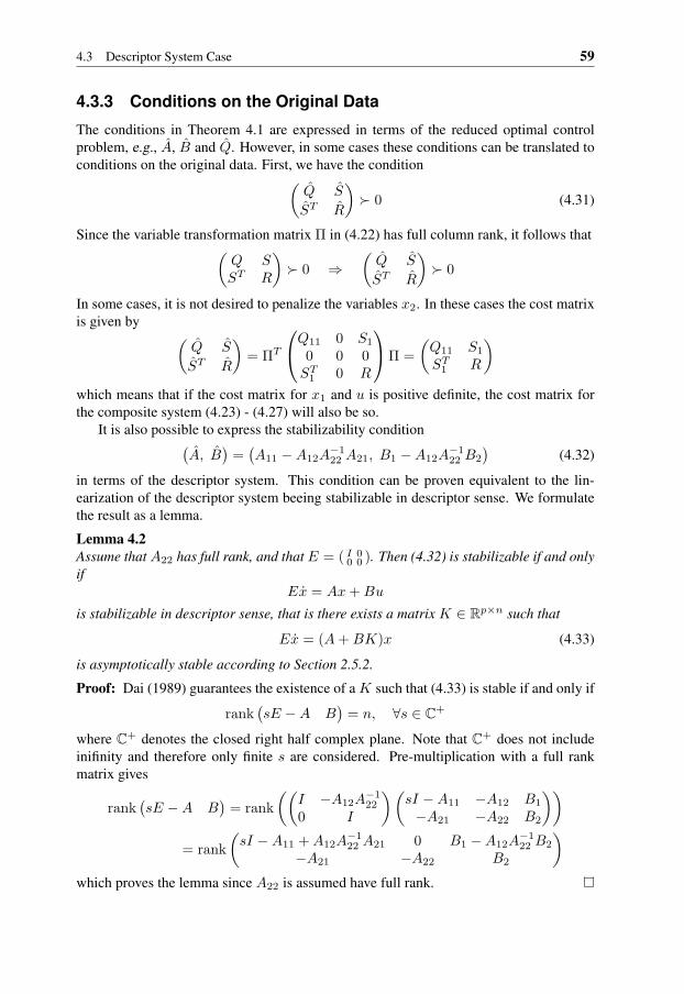
4.3 Descriptor System Case 59
4.3.3 Conditions on the Original Data
The conditions in Theorem 4.1 are expressed in terms of the reduced optimal controlproblem, e.g., A, B and Q. However, in some cases these conditions can be translated toconditions on the original data. First, we have the condition(
Q S
ST R
) 0 (4.31)
Since the variable transformation matrix Π in (4.22) has full column rank, it follows that(Q SST R
) 0 ⇒
(Q S
ST R
) 0
In some cases, it is not desired to penalize the variables x2. In these cases the cost matrixis given by (
Q S
ST R
)= ΠT
Q11 0 S1
0 0 0ST
1 0 R
Π =(Q11 S1
ST1 R
)which means that if the cost matrix for x1 and u is positive definite, the cost matrix forthe composite system (4.23) - (4.27) will also be so.
It is also possible to express the stabilizability condition(A, B
)=(A11 −A12A
−122 A21, B1 −A12A
−122 B2
)(4.32)
in terms of the descriptor system. This condition can be proven equivalent to the lin-earization of the descriptor system beeing stabilizable in descriptor sense. We formulatethe result as a lemma.
Lemma 4.2Assume that A22 has full rank, and that E = ( I 0
0 0 ). Then (4.32) is stabilizable if and onlyif
Ex = Ax+Bu
is stabilizable in descriptor sense, that is there exists a matrix K ∈ Rp×n such that
Ex = (A+BK)x (4.33)
is asymptotically stable according to Section 2.5.2.
Proof: Dai (1989) guarantees the existence of a K such that (4.33) is stable if and only if
rank(sE −A B
)= n, ∀s ∈ C+
where C+ denotes the closed right half complex plane. Note that C+ does not includeinifinity and therefore only finite s are considered. Pre-multiplication with a full rankmatrix gives
rank(sE −A B
)= rank
((I −A12A
−122
0 I
)(sI −A11 −A12 B1
−A21 −A22 B2
))= rank
(sI −A11 +A12A
−122 A21 0 B1 −A12A
−122 B2
−A21 −A22 B2
)which proves the lemma since A22 is assumed have full rank.

60 4 Power Series Solution of the Hamilton-Jacobi-Bellman Equation
Algorithm 4.1 Computation of the locally optimal solution
1. Compute the series expansion of the system and performance criterion using (4.5).
2. Compute ϕ[1](x1, u) as described in (4.19) to obtain the expressions for A and B.
3. Solve (4.27) to obtain V [2](x1) = xT1 Px1 and u[1]
∗ (x1) = D∗x1. Use these expres-sions to compute ϕ[1](x1, u
[1]∗ ). Let m = 3.
4. Compute
F[m−1]1h (x1, u∗) = F
[m−1]1h (x1, u
[1]∗ + . . .+ u
[m−2]∗ )
L[m]h (x1, u∗) = L
[m]h (x1, u
[1]∗ + . . .+ u
[m−2]∗ )
using (4.29) and solve (4.28a) to obtain V [m](x1).
5. Having V [m](x1) and after computation of
F[m−2]1h;u (x1, u∗) = F
[m−2]1h;u (x1, u
[1]∗ + . . .+ u
[m−2]∗ )
L[m−1]h;u (x1, u∗) = L
[m−1]h;u (x1, u
[1]∗ . . .+ u
[m−2]∗ )
using (4.30), u[m−1]∗ (x1) can be obtained from (4.28b).
6. Compute ϕ[m−1](x1, u) from (4.21) and use it to compute
ϕ[m−1](x1, u∗) = ϕ[m−1](x1, u[1]∗ . . .+ u
[m−1]∗ )
7. If a higher order approximation is desired, increase m by one and repeat from step4.
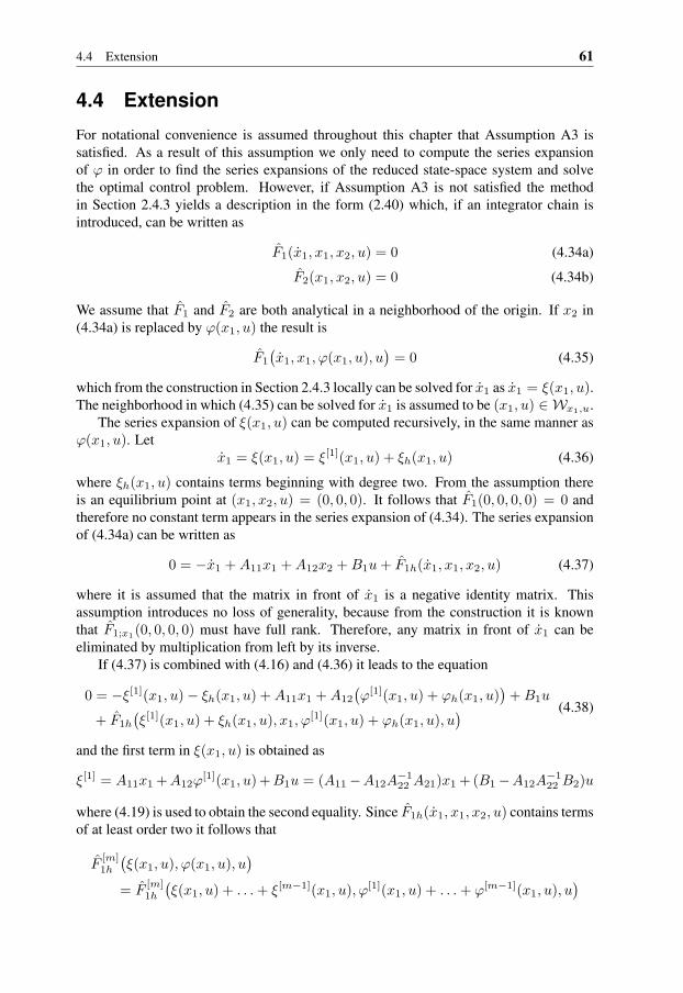
4.4 Extension 61
4.4 Extension
For notational convenience is assumed throughout this chapter that Assumption A3 issatisfied. As a result of this assumption we only need to compute the series expansionof ϕ in order to find the series expansions of the reduced state-space system and solvethe optimal control problem. However, if Assumption A3 is not satisfied the methodin Section 2.4.3 yields a description in the form (2.40) which, if an integrator chain isintroduced, can be written as
F1(x1, x1, x2, u) = 0 (4.34a)
F2(x1, x2, u) = 0 (4.34b)
We assume that F1 and F2 are both analytical in a neighborhood of the origin. If x2 in(4.34a) is replaced by ϕ(x1, u) the result is
F1
(x1, x1, ϕ(x1, u), u
)= 0 (4.35)
which from the construction in Section 2.4.3 locally can be solved for x1 as x1 = ξ(x1, u).The neighborhood in which (4.35) can be solved for x1 is assumed to be (x1, u) ∈ Wx1,u.
The series expansion of ξ(x1, u) can be computed recursively, in the same manner asϕ(x1, u). Let
x1 = ξ(x1, u) = ξ[1](x1, u) + ξh(x1, u) (4.36)
where ξh(x1, u) contains terms beginning with degree two. From the assumption thereis an equilibrium point at (x1, x2, u) = (0, 0, 0). It follows that F1(0, 0, 0, 0) = 0 andtherefore no constant term appears in the series expansion of (4.34). The series expansionof (4.34a) can be written as
0 = −x1 +A11x1 +A12x2 +B1u+ F1h(x1, x1, x2, u) (4.37)
where it is assumed that the matrix in front of x1 is a negative identity matrix. Thisassumption introduces no loss of generality, because from the construction it is knownthat F1;x1(0, 0, 0, 0) must have full rank. Therefore, any matrix in front of x1 can beeliminated by multiplication from left by its inverse.
If (4.37) is combined with (4.16) and (4.36) it leads to the equation
0 = −ξ[1](x1, u)− ξh(x1, u) +A11x1 +A12
(ϕ[1](x1, u) + ϕh(x1, u)
)+B1u
+ F1h
(ξ[1](x1, u) + ξh(x1, u), x1, ϕ
[1](x1, u) + ϕh(x1, u), u) (4.38)
and the first term in ξ(x1, u) is obtained as
ξ[1] = A11x1 +A12ϕ[1](x1, u)+B1u = (A11−A12A
−122 A21)x1 +(B1−A12A
−122 B2)u
where (4.19) is used to obtain the second equality. Since F1h(x1, x1, x2, u) contains termsof at least order two it follows that
F[m]1h
(ξ(x1, u), ϕ(x1, u), u
)= F
[m]1h
(ξ(x1, u) + . . .+ ξ[m−1](x1, u), ϕ[1](x1, u) + . . .+ ϕ[m−1](x1, u), u
)

62 4 Power Series Solution of the Hamilton-Jacobi-Bellman Equation
Hence, it is possible to compute ξ(x1, u) recursively. The series expansion obtained fitsinto earlier described results, and the computation order for the optimal control problembecomes
V [2](x1), u[1]∗ (x1), ϕ[1](x1, u
[1]∗ ), ξ[1](x1, u
[1]∗ ) . . .
As an result, it is possible to compute the optimal solution for systems which is given onthe more general form (4.34), i.e., not satisfying Assumption A3, with the method derivedin this chapter.
4.5 Example
In order to illustrate the method we will study a small example. The system dynamics aregiven by
z1 = z2
z2 = ez3 − 1 +12u
0 = z1 − arcsin(1− ez3 +12u)
(4.39)
consisting of both differential and algebraic equations. The physical interpretation of(4.39) is a Phase-Locked Loop circuit (PLL) which is used to control an oscillator so thatit maintains a constant phase angle relative to a reference signal. The objective is to findthe feedback law (4.3) which minimizes a performance criterion with the cost functionchosen as
L(z1, z2, z3, u) =12z21 + 2z1z2 + z2
2 + z1(−ez3 + 1 +12u) +
12u2 (4.40)
When the variables are grouped according to x1 = (z1, z2)T and x2 = z3, the system is
in semi-explicit form, with
F1(z1, z2, z3, u) =(
z2ez3 − 1 + 1
2u
)F2(z1, z2, z3, u) = z1 − arcsin(1− ez3 +
12u)
and E =(
1 0 00 1 00 0 0
). Expressing the descriptor system in the form (4.5a) by computing the
power series expansion of F1(z1, z2, z3, u) and F2(z1, z2, z3, u) around the origin yieldsthe first order terms
A =
0 1 00 0 11 0 1
, B =
01/2−1/2
(4.41)
and the higher order terms of order up till three as
F1h(z1, z2, z3, u) =(
01/2z2
3 + 1/6z33
)(4.42a)
F2h(z1, z2, z3, u) = 1/2z23 + 1/3z3
3 − 1/4uz23 + 1/8u2z3 − 1/48u3 (4.42b)
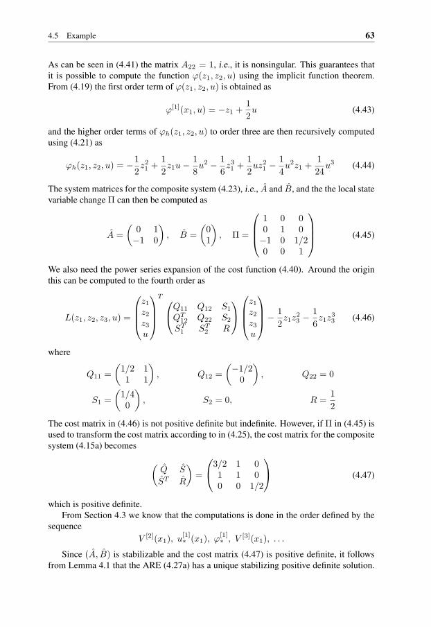
4.5 Example 63
As can be seen in (4.41) the matrix A22 = 1, i.e., it is nonsingular. This guarantees thatit is possible to compute the function ϕ(z1, z2, u) using the implicit function theorem.From (4.19) the first order term of ϕ(z1, z2, u) is obtained as
ϕ[1](x1, u) = −z1 +12u (4.43)
and the higher order terms of ϕh(z1, z2, u) to order three are then recursively computedusing (4.21) as
ϕh(z1, z2, u) = −12z21 +
12z1u−
18u2 − 1
6z31 +
12uz2
1 −14u2z1 +
124u3 (4.44)
The system matrices for the composite system (4.23), i.e., A and B, and the the local statevariable change Π can then be computed as
A =(
0 1−1 0
), B =
(01
), Π =
1 0 00 1 0−1 0 1/20 0 1
(4.45)
We also need the power series expansion of the cost function (4.40). Around the originthis can be computed to the fourth order as
L(z1, z2, z3, u) =
z1z2z3u
T Q11 Q12 S1
QT12 Q22 S2
ST1 ST
2 R
z1z2z3u
− 12z1z
23 −
16z1z
33 (4.46)
where
Q11 =(
1/2 11 1
), Q12 =
(−1/2
0
), Q22 = 0
S1 =(
1/40
), S2 = 0, R =
12
The cost matrix in (4.46) is not positive definite but indefinite. However, if Π in (4.45) isused to transform the cost matrix according to in (4.25), the cost matrix for the compositesystem (4.15a) becomes (
Q S
ST R
)=
3/2 1 01 1 00 0 1/2
(4.47)
which is positive definite.From Section 4.3 we know that the computations is done in the order defined by the
sequenceV [2](x1), u
[1]∗ (x1), ϕ
[1]∗ , V
[3](x1), . . .
Since (A, B) is stabilizable and the cost matrix (4.47) is positive definite, it followsfrom Lemma 4.1 that the ARE (4.27a) has a unique stabilizing positive definite solution.
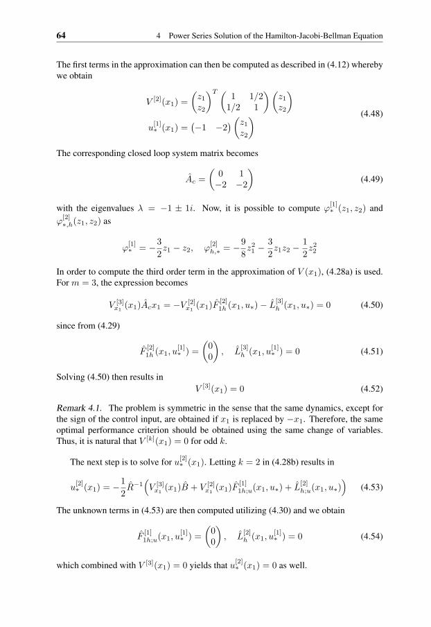
64 4 Power Series Solution of the Hamilton-Jacobi-Bellman Equation
The first terms in the approximation can then be computed as described in (4.12) wherebywe obtain
V [2](x1) =(z1z2
)T ( 1 1/21/2 1
)(z1z2
)u
[1]∗ (x1) =
(−1 −2
)(z1z2
) (4.48)
The corresponding closed loop system matrix becomes
Ac =(
0 1−2 −2
)(4.49)
with the eigenvalues λ = −1 ± 1i. Now, it is possible to compute ϕ[1]∗ (z1, z2) and
ϕ[2]∗,h(z1, z2) as
ϕ[1]∗ = −3
2z1 − z2, ϕ
[2]h,∗ = −9
8z21 −
32z1z2 −
12z22
In order to compute the third order term in the approximation of V (x1), (4.28a) is used.For m = 3, the expression becomes
V [3]x1
(x1)Acx1 = −V [2]x1
(x1)F[2]1h (x1, u∗)− L
[3]h (x1, u∗) = 0 (4.50)
since from (4.29)
F[2]1h (x1, u
[1]∗ ) =
(00
), L
[3]h (x1, u
[1]∗ ) = 0 (4.51)
Solving (4.50) then results inV [3](x1) = 0 (4.52)
Remark 4.1. The problem is symmetric in the sense that the same dynamics, except forthe sign of the control input, are obtained if x1 is replaced by −x1. Therefore, the sameoptimal performance criterion should be obtained using the same change of variables.Thus, it is natural that V [k](x1) = 0 for odd k.
The next step is to solve for u[2]∗ (x1). Letting k = 2 in (4.28b) results in
u[2]∗ (x1) = −1
2R−1
(V [3]
x1(x1)B + V [2]
x1(x1)F
[1]1h;u(x1, u∗) + L
[2]h;u(x1, u∗)
)(4.53)
The unknown terms in (4.53) are then computed utilizing (4.30) and we obtain
F[1]1h;u(x1, u
[1]∗ ) =
(00
), L
[2]h (x1, u
[1]∗ ) = 0 (4.54)
which combined with V [3](x1) = 0 yields that u[2]∗ (x1) = 0 as well.
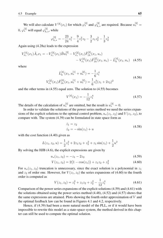
4.5 Example 65
We will also calculate V [4](x1) for which ϕ[2]∗ and ϕ[3]
h,∗ are required. Because u[2]∗ =
0, ϕ[2]∗ will equal ϕ[2]
h,∗, while
ϕ[3]h,∗ = −23
24z31 −
94z21z2 −
32z1z
22 −
13z32
Again using (4.28a) leads to the expression
V [4]x1
(x1)Acx1 = −V [3]x1
(x1)Bu[2]∗ − V [2]
x1(x1)F
[3]1h (x1, u∗)
− V [3]x1
(x1)F[2]1h (x1, u∗)− L
[4]h (x1, u∗) (4.55)
where
L[4]h (x1, u
[1]∗ + u
[2]∗ ) = −1
6z41
V [2]x1
(x1)F[3]1h (x1, u
[1]∗ + u
[2]∗ ) =
16z31(z1 + 2z2)2
(4.56)
and the other terms in (4.55) equal zero. The solution to (4.55) becomes
V [4](x1) = − 112z41 (4.57)
The details of the calculation of u[3]∗ are omitted, but the result is u[3]
∗ = 0.In order to validate the solutions of the power series method we need the series expan-
sions of the explicit solutions to the optimal control problem, u∗(z1, z2) and V (z1, z2), tocompare with. The system (4.39) can be formulated in state space form as
z1 = z2
z2 = − sin(z1) + u(4.58)
with the cost function (4.40) given as
L(z1, z2, u) =12z21 + 2z1z2 + z2
2 + z1 sin(z1) +12u2
By solving the HJB (4.6), the explicit expressions are given by
u∗(z1, z2) = −z1 − 2z2 (4.59)
V (z1, z2) = 2(1− cos(z1)
)+ z1z2 + z2
2 (4.60)
For u∗(z1, z2) truncation is unnecessary, since the exact solution is a polynomial in z1and z2 of order one. However, for V (z1, z2) the series expansions of (4.60) to the fourthorder is computed as
V (z1, z2) = z21 + z1z2 + z2
2 −112z41 (4.61)
Comparison of the power series expansions of the explicit solutions (4.59) and (4.61) withthe solutions obtained using the power series method (4.48), (4.52) and (4.57) shows thatthe same expressions are attained. Plots showing the fourth order approximation of V andthe optimal feedback law can be found in Figures 4.1 and 4.2, respectively.
Hence, if (4.39) had been a more natural model of the PLL, or if it would have beenimpossible to rewrite this model as a state-space system, the method derived in this chap-ter can still be used to compute the optimal solution.
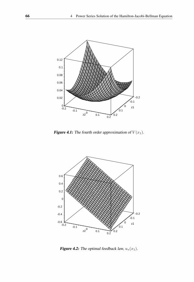
66 4 Power Series Solution of the Hamilton-Jacobi-Bellman Equation
-0.2
-0.1
0-0.20
z1
0.02
-0.1
0.04
0.1
0.06
0
0.08
z2 0.1
0.1
0.2
0.12
0.2
Figure 4.1: The fourth order approximation of V (x1).
-0.2
-0.1
0-0.2
-0.6z1
-0.4
-0.1
-0.2
0.1
0
0
0.2
z2 0.1
0.4
0.2
0.6
0.2
Figure 4.2: The optimal feedback law, u∗(x1).

5Controllability Function
In this chapter the controllability function for nonlinear descriptor systems is considered.The controllability function describes the minimum amount of control energy required toreach a specific state in infinite time. That is, a large value means that the specific stateis difficult to reach. As the formulation suggests, the controllability function is defined asthe solution to an optimal control problem where the performance criterion is an energymeasure of the control input.
For state-space systems the controllability function is studied in Scherpen (1994) andreferences therein. Scherpen shows that for linear time-invariant state-space systems thecontrollability function is given by the inverse of the controllability gramian multipliedfrom the left and right by the state. The connection between a finite, nonzero controllabil-ity function and different concepts of controllability for control-affine nonlinear systemsis to some extent studied in, e.g., Scherpen and Gray (2000).
The controllability function for regular time-invariant linear descriptor systems withconsistent initial conditions, has been considered in Stykel (2004). The method suggestedby Stykel can also be used to handle systems that for a given input u(t) have higher index,without first using index reduction.
For nonlinear descriptor systems, Lin and Ahmed (1991) consider controllability us-ing the maximum principle. However, they do not formulate the controllability function,but instead formulate the controllability problem as a feasibility problem which is solvedusing optimal control.
The optimal control problem for the controllability function is in this chapter solvedusing the results obtained in Chapter 3 and Chapter 4. Three different methods are de-rived. In Section 5.2, a method is derived based on the necessary conditions for optimalitygiven by the Hamilton-Jacobi-Bellman theory in Chapter 3. The second method can befound in Section 5.3. It is based on an approach similar to the one used by Scherpen(1994). It uses completion of squares and is applicable because the performance criteriononly includes the term uTu. These two methods find the controllability function on some
67
68 5 Controllability Function
set x1 ∈ Ωx. The third method, presented in Section 5.4, finds a local controllabilityfunction, i.e., a controllability function valid in a neighborhood of the origin. The lastmethod can also be used to find an approximation for the controllability function.
5.1 Problem Formulation
A general controllability function should basically measure the minimal amount of energyin the control signal u(t) required to reach a specific state x. Therefore, it is necessary todefine a measure of the control signal energy. The most common energy measure, see forexample Scherpen (1994), and the energy measure used in this thesis is
Jc =
0∫−∞
m(u(t)
)dt =
12
0∫−∞
u(t)Tu(t) dt (5.1)
It would be possible to use a more generalm(u(t)
), but in order to get a nice interpretation
it has to be positive definite, i.e., satisfying m(u(t)
)> 0 for all nonzero u(t).
The controllability function Lc(x1) is defined as the solution to the optimal controlproblem
Lc
(x1(0)
)= min
u(·)Jc (5.2)
subject to the system dynamics
x1 = F1(x1, x2, u) (5.3a)0 = F2(x1, x2, u) (5.3b)
and the boundary conditions
x1(0) = x1,0 ∈ Ωx
limt→−∞
x1(t) = 0
The system dynamics are, as in the other chapters, assumed to be in semi-explicitform and to have an equilibrium at the origin. However, different assumptions regardingthe implicit function will be made in different sections. In Section 5.2 and Section 5.3,Assumption A2 is made, while in Section 5.4, Assumption A4 is used instead. In bothcases it is known that x2 = ϕ(x1, u) for x1 ∈ Ωx and the difference is the assumption onthe region for u.
The controllability function must satisfy the condition Lc(0) = 0. The reason is theinterpretation of Lc(x1,0) as the minimum amount of input energy required to drive thesystem from zero at t = −∞ to x1(0) = x1,0 at t = 0. According to the assumptions,the system (5.3) has an equilibrium in the origin and since no control effort is neededto keep x = 0 the energy then equals zero. We also use a convention that if x0 cannotbe asymptotically reached from 0, i.e., if no control input such that x1(−∞) = 0 andx1(0) = x1,0 exists, Lc(x1,0) is infinite.
5.2 Method Based on HJB Theory 69
The boundary conditions on x1 implies that the control input u(·) must make theclosed loop system asymptotically anti-stable for x1,0 ∈ Ωx. That is, if the time is re-versed and instead is considered as going from 0 towards −∞, the closed loop systemmust be asymptotically stable.
We will only consider controllability on the set
N = x1 ∈ Ωx, x2 ∈ Rn2 |x2 = ϕ(x1, u), u ∈ Ωu
where Ωu is either Rp or a neighborhood of u = 0 depending on the assumption made.This means that, only controllability on the set of points not violating the constraints areconsidered. This is assured by choosing the final state x1,0 in Ωx. Note that if it is possibleto reach all x1,0 ∈ Ωx, it is also possible to reach all (x1,0, x2,0) ∈ N . The reason is thatit is possible to use some u(t) for −∞ < t < 0 and then at t = 0 use u(0) to obtainx2(0) = x2,0. This does not change the value of the performance criterion.
5.2 Method Based on HJB Theory
In this section the system is assumed to satisfy Assumption A2, that is Ωu = Rp. The op-timal control problem (5.2) can then be seen as a special case of the problems consideredin Chapter 3 with the cost function
L(x1, x2, u) =12uTu (5.4)
However, since the final state and not the initial state is specified, the time in (5.2) can beconsidered as going backwards compared to (3.3). This fact leads to the change of somesigns in the Hamilton-Jacobi-like equation (3.8), and the result is the equation
0 = minu
(12uTu−W1(x1)F1(x1, x2, u)−W2(x1, x2)F2(x1, x2, u)
)(5.5)
where W1(x1) and W2(x1, x2) are continuous functions such that W1(x1) is the gradientof some continuously differentiable function V (x1).
The necessary conditions for optimality corresponding to (5.5) can be found in Sec-tion 3.3. However, due to the structure of the cost function, the conditions can be some-what simplified. We formulate the conditions as a proposition.
Proposition 5.1Consider the optimal control problem (5.2) under Assumption A2. Then the optimal solu-tion must satisfy
0 = uT −W1(x1)F1;u(x1, x2, u)−W2(x1, x2)F2;u(x1, x2, u) (5.6a)
0 =12uTu−W1(x1)F1(x1, x2, u) (5.6b)
0 = F2(x1, x2, u) (5.6c)
0 = W2(x1, x2) +W1(x1)F1;x2(x1, x2, u)F−12;x2
(x1, x2, u) (5.6d)
for x1 ∈ Ωx.
70 5 Controllability Function
Proof: Follows immediately from the conditions in Section 3.3.
In Proposition 5.1, (5.6d) is included since the system is assumed to satisfy Assump-tion A2.
Remark 5.1. In Section 3.5 a special case was considered where the system is given by
x1 = f1(x1, x2) + g1(x1)u (5.7a)0 = f2(x1, x2) + g2(x1)u (5.7b)
In this case, for which the necessary conditions became extra simple. In the controlla-bility function setup the equations obtained in Section 3.5 can be even more simplified.First notice that f2,x2(x1, x2) is nonsingular for all (x1, x2) such that f2(x1, x2) = 0 issolvable since F2;x2(x1, x2, u) is nonsingular for all (x1, x2, u) ∈ Ω and then particularlyfor u = 0.
Using (5.6d) an expression for W2(x1, x2) can be formulated as
W2(x1, x2) = −W1(x1)f1;x2(x1, x2)f−12;x2
(x1, x2)
Combining this expression with (5.6a) yields
u = g(x1, x2)TW1(x1)T
and after some more manipulations the necessary conditions can be rewritten as
0 = W1(x1)f(x1, x2) +12W1(x1)g(x1, x2)g(x1, x2)TW1(x1)T (5.8a)
0 = f2(x1, x2) + g2(x1)g(x1, x2)TW1(x1)T (5.8b)
where
f(x1, x2) = f1(x1, x2)− f1;x2(x1, x2)f−12;x2
(x1, x2)f2(x1, x2)
g(x1, x2) = g1(x1)− f1;x2(x1, x2)f−12;x2
(x1, x2)g2(x1)
Hence, the original four equations with four unknowns are reduced to the two equa-tions (5.8) and the two unknowns W1(x1) and x2 = η(x1).
5.3 Method Based on Completion of Squares
The HJB equation yields both necessary and sufficient conditions for optimality. How-ever, when differentiation with respect to u is used to find the optimal control, sufficiencyis lost and only necessary conditions are obtained.
In this section the class of systems considered is limited to systems in the form
Ex = f(x) + g(x)u (5.9)
where E =(
In1 00 0
). For the considered class of systems it is possible to use another
approach to show optimality. The approach is to a large extent similar to the approachin Scherpen (1994) and uses the fact that the performance criterion only depends on thesquared control signal, i.e., uTu. The advantage of this approach is that sufficient condi-tions for optimality are obtained. The result is stated in Theorem 5.1.

5.3 Method Based on Completion of Squares 71
Theorem 5.1Suppose there exist continuous functions W1(x1) = Vx1(x1) and W2(x1, x2) such thatLc(x) =
(W1(x1), W2(x1, x2)
)fulfills
0 = Lc(x)f(x) +12Lc(x)g(x)g(x)T Lc(x)T (5.10)
for all x ∈ N . Furthermore, assume that for the control choice
u = g(x)T Lc(x)T (5.11)
the system (5.9) can be solved backwards in time from t = 0, with x(t) → 0, t → −∞.Under these conditions, Lc(x1) = V (x1) and the corresponding u is the optimal controllaw.
Proof: Assume that x1,0 ∈ Ωx. For any control signal u(·) such that the solution to (5.9)fulfills x(t) → 0 as t→ −∞ it follows that
12
0∫−∞
uTu dt = V (x1(0)) +
0∫−∞
(12uTu− Vx1(f1 + g1u)−W2(f2 + g2u)
)dt
where V (x1), W2(x1, x2) are arbitrary sufficiently smooth functions. Completing thesquares gives
12
0∫−∞
uTu dt = V(x1(0)
)+
0∫−∞
12‖u− g(x)T Lc(x)T ‖2 dt
provided (5.10) is satisfied. It can be realized that V(x1(0)
)is a lower bound for the
integral in (5.1). By choosing u = g(x)T Lc(x)T this lower bound is obtained and sincethis control choice is such that the closed loop system can be solved backwards in timeand x(−∞) = 0, it is optimal. Therefore, for all x1,0 ∈ Ωx
Lc(x1,0) = minu(·)
12
0∫−∞
uTu dt = V (x1,0)
Note that the proof above assumes that Ωx is an invariant set for the closed loopsystem. However, since the closed loop system is asymptotically anti-stable such a choiceof Ωx can always be done, as was shown in Section 2.5.1.
The requirement that the closed loop system, using (5.11) must be asymptoticallystable going backwards in time for x ∈ N is equivalent to
E ˙x = −(f(x) + g(x)g(x)T Lc(x)T
)(5.12)
being asymptotically stable on Ωx, where x(s) = x(−s) and s = −t. To verify that (5.12)is asymptotically stable, the methods described in Section 2.6 can be used.
72 5 Controllability Function
Theorem 5.1 is primarily intended to verify optimality and not to calculate W1 andW2. This can be realized since it is assumed that W1 and W2 are known beforehand.Therefore, a good idea if in the case when the system fits into (5.9) is to combine themethod in this section with the method in Section 5.2. First candidate solutions are foundusing the necessary conditions and the optimal solution is then chosen using Theorem 5.1.The approach is illustrated in Example 5.6.1.
5.4 Method to Find a Local Solution
In Chapter 4 it was shown how to compute a local solution to an optimal control prob-lem. The solution was expressed as a power series expansion and as long as it was nottruncated, it was the true optimal solution. In this section, we use the same approach forthe controllability function computation. However, minor changes of the assumptions onthe cost function are needed. In Chapter 4, and more specifically Theorem 4.1, the costfunction L(x1, u) is assumed to be positive definite in both x1 and u locally around theorigin. In the calculation of the controllability function, x1 and x2 do not appear in thecost function and the cost function can therefore not be positive definite. However, us-ing slightly different requirements, it is still possible to guarantee the existence of a localoptimal solution in a neighborhood of the origin, i.e., a local controllability function.
5.4.1 Basic Assumptions and Formulations
The objective is to find the controllability function expressed as a convergent power seriesexpansion
Lc(x1) =12xT
1 Gcx1 + Lch(x1) (5.13)
where Lch(x1) contains higher order terms at least of order three.The considered class of control inputs can also be written as a convergent power series
u(x1) = Dx1 + uh(x1) (5.14)
where uh(x1) is higher order terms of order two or higher. The feedback law only dependson x1, which is known since the system (5.3) is assumed to satisfy Assumption A4 (cf.Section 4.3). To be able to express F = (FT
1 , FT2 )T as a convergent series expansions,
it is assumed that F satisfies Assumption A5, i.e., is analytical on some set W , whereW is given in (4.4). Under this assumption, F (x1, x2, u) can be expressed as describedin (4.5a).
The cost function is already expressed as a convergent power series, since
L(x1, x2, u) =12uTu (5.15)
The corresponding cost matrix is(Q SST R
)=(
0 00 1/2I
)and no higher order terms exist, i.e., Lh(x1, x2, u) = 0.
5.4 Method to Find a Local Solution 73
The series expansion of the reduced system can be found in the same manner as inChapter 4. However, since the boundary condition on x1 is the final state and not theinitial state, time must be considered as going backwards compared to the optimal controlproblem (4.2). Therefore, when using the results in Chapter 4, the system (4.23) will be
x1 = −Ax1 − Bu− F1h(x1) (5.16)
where A = A11 − A12A−122 A21, B = B1 − A12A
−122 B2 and F1h(x1) is found in (4.24).
That is, the signs have changed.The reduced cost function L will in this case be very simple since L depends on
neither x1 nor x2. Therefore, L is given by
L(u) =12uTu (5.17)
which yields the cost matrix (Q S
ST R
)=(
0 00 1/2I
)(5.18)
and no higher order terms, i.e., Lh(u) = 0. The lack of higher order terms also leads toLh;u(u) = 0.
One assumption in the problem formulation, presented in Section 5.1, is that the con-trol input must be chosen such that the closed loop system is made asymptotically anti-stable. This is equivalent to that the closed loop system in backward time is asymptoticallystable. In this case, the system going backwards in time is given by (5.16) and since onlylocal properties are considered, a sufficient condition for the control input (5.14) is that−A− BD is Hurwitz, i.e., <λi(−A− BD) < 0 for i = 1, . . . , n1. We formulate this asan assumption.
Assumption A6. Only matrices D such that −A− BD is Hurwitz are considered.
5.4.2 Application of the Local Method
Using the information in the previous section, it is possible to modify the results in Chap-ter 4 so that the results can be used to find the controllability function. In this section wederive the new equations and a new existence theorem.
Using (4.27), the equations for the lowest order terms of (5.13) and (5.14), i.e., Gc
and D∗, respectively, are obtained as
GcA+ ATGc +GcBBTGc = 0 (5.19a)
D∗ − BTGc = 0 (5.19b)
The equations for the higher order terms of Lc(x1) are obtained from (4.28a) as
L[m]c;x1
(x1)Acx1 =
−m−1∑k=3
L[k]c;x1
(x1)Bu[m−k+1]∗ (x1)−
m−1∑k=2
L[k]c;x1
(x1)F[m−k+1]1h (x1, u∗)
+bm−1
2 c∑k=2
u[k]∗ (x1)Tu
[m−k]∗ (x1) +
12u
[m/2]∗ (x1)Tu
[m/2]∗ (x1)
(5.20a)
74 5 Controllability Function
where m = 3, 4, . . ., Ac = A + BD∗, and the terms u[m/2] are to be omitted if m isodd. The corresponding equation for the series expansion of the feedback law is obtainedfrom (4.28b) as
u[k]∗ (x1) = L[k+1]
c;x1(x1)B +
k−1∑i=1
L[k−i+1]c;x1
(x1)F[i]1h,u(x1, u∗) (5.20b)
where k = 2, 3, . . ..The equations in (5.20) are very similar to the original equations in Chapter 4, how-
ever, the computation of the equations above are less involved. The reason lies in theexpressions for Lh and Lh;u. In Chapter 4, these expressions are given by (4.29b) and(4.30b), respectively, which are rather involved, while in this chapter both of these arezero.
As can be seen in Theorem 4.1, a fundamental assumption in Chapter 4 was a positivedefinite cost matrix (5.18). However, this requirement is not satisfied in calculation of thecontrollability function. The results in Chapter 4 are based on the proof in Lukes (1969).Careful examination of the proof shows that most parts still hold when x is not presentin the cost function as long as R is positive definite, which is satisfied in the computationof the controllability function. However, two statements rely on positive definiteness of(5.18). First, the argument that the second order term in the optimal performance criterionis positive definite. This fact is used to determine which solution to the ARE (4.10a) isoptimal. Second, the assertion that the ARE (4.10a) has a unique positive definite solution,which moreover locally stabilizes the closed loop system. We therefore need to investigatewhich properties Gc will have when the cost function is given by (5.18), and under whichconditions the ARE (5.19a) has a stabilizing solution such that the properties of Gc aresatisfied.
The two parts that does obviously hold in the proof by Lukes (1969) is reformulatedin the following lemmas.
Lemma 5.1Given an asymptotically stable matrix A and a matrix D such that −A− BD is Hurwitz,the matrix Gc in the controllability function (5.13) is positive semidefinite.
Proof: From Lukes (1969) it is known that if we consider systems given by (5.16) andfeedback laws (5.14) such that −A − BD is Hurwitz, the matrix P in a general optimalcontrol problem, described in Chapter 4, is given by
P =
∞∫0
e(−A−BD)T t(Q+ SD +DT ST +DTD
)e(−A−BD)t dt
In the controllability function case, where the cost matrix is given by (5.18), it followsthat
Gc =
∞∫0
e(−A−BD)T tDTDe(−A−BD)t dt
which obviously is positive semidefinite.

5.4 Method to Find a Local Solution 75
Lemma 5.1 is rather simple, but is formulated to show the difference compared toLukes (1969). If necessary, Lemma 5.1 can be strengthened to guaranteeGc 0, howeverthis is not needed to determine which of the solutions to the necessary conditions foroptimality that is optimal.
The lemma below states when the ARE (5.19a) can be expected to have a solutionsuch that Gc becomes at least positive semidefinite and D∗ becomes stabilizing.
Lemma 5.2Assume that A is Hurwitz and (A, B) is controllable. Then the ARE
0 = ATGc +GcA+GcBBTGc (5.21)
has a unique positive definite solution Gc such that Ac,b = −A − BBTGc is Hurwitz.Furthermore, Gc is the only positive semidefinite solution such that Ac,b is Hurwitz.
Proof: The ARE in (5.21) is somewhat special since it has no constant term. Therefore,Gc = 0 is always a solution. However, for the given assumptions Gc = 0 can never makeAc,b Hurwitz, since A is Hurwitz.
From the assumptions it follows that: a) (−A,−B) is stabilizable, because (A, B)is controllable, b) (−A, 0) has no undetectable modes on the imaginary axis, because Ais asymptotic stable. According to Bittanti et al. (1991), a) and b) combined will yieldthat (5.21) has a unique maximal positive definite solution, Gc. Moreover, this solution issuch that Ac,b is Hurwitz.
The stabilizing solution Gc, is also the only positive definite solution. To show this,first note that for all Gc 0, (5.21) can be reformulated as a Lyapunov equation
0 = AG−1c +G−1
c AT + BBT
Hence, all positive definite solutions to the ARE are positive definite solutions to theLyapunov equation and vice versa. It is well-known that the Lyapunov equation has aunique positive definite solution if A is asymptotically stable and (A, B) is controllable,see for example Kailath et al. (2000). Therefore, Gc 0 must be unique.
Finally, according to Bittanti et al. (1991) all other positive semidefinite solutionsto (5.21) are such that Ac,b will have some eigenvalues with positive real part, whichproves the last statement in the theorem.
The last statement, i.e., thatGc is the only stabilizing solution which is at least positivesemidefinite, is important. The reason is that we have not showed thatGc must be positivedefinite in order to be optimal, and instead the stability requirement is used to select theoptimal solution.
The results in this section is summarized in the following theorem.
Theorem 5.2Assume that the system (5.3) satisfies Assumptions A4, A5 and A6. Furthermore, assumethat A is Hurwitz and (A, B) is controllable. Then the system has a local controllabilityfunction given by
Lc(x1) =12xT
1 Gcx1 + Lch(x1)
76 5 Controllability Function
where Gc is the unique positive definite solution to the ARE (5.19a) such that D∗, givenby (5.19b), makes −A− BD∗ Hurwitz.
The higher order terms Lch(x1) and uh,∗ are given as the unique solutions to (5.20).
Proof: According to the assumptions, A is Hurwitz and only matrices D such that−A−BD is Hurwitz are considered. Lemma 5.1 then guarantees that the optimal solution Gc
will be positive semidefinite.With A Hurwitz and (A, B) controllable, it follows from Lemma 5.2 that a unique
positive definite solutionGc exists such that all eigenvalues to−A−BBTGc have strictlynegative real parts. Moreover, all other positive semidefinite solutions to the ARE (5.19a)are such that at least some eigenvalue to −A− BBTGc have a nonnegative real part.
Hence, using D∗ from (5.19b) the only positive semidefinite solution such that As-sumption A6 is satisfied, i.e., such that −A − BD∗ is Hurwitz, is Gc. The first terms inthe optimal solution must therefore beGc andD∗. When−A−BD∗ is Hurwitz, (5.20a) isuniquely solvable for a given right-hand side, see for example Lyapunov (1992). There-fore, by choosing the unique positive definite solution to the ARE, the controllabilityfunction is found.
Remark 5.2. The local controllability function satisfies Lc(x1) > 0 for all nonzero x1 insome neighborhood of the origin.
Remark 5.3. The extension in Section 4.4 can be used also in the computation of thecontrollability function to handle a more general class of systems.
As in Chapter 4 the conditions in Theorem 5.2 are formulated in terms of the reducedsystem. Controllability of (A, B) is equivalent to R-controllability of (A,B). This canbe proven in a very similar way to the proof regarding stabilizability, see Section 4.3.3 orDai (1989).
5.5 Linear Descriptor Systems
In this section the methods described in Sections 5.1 and 5.3, are applied to linear descrip-tor systems. It should be pointed out that the purpose is just to show these methods. Thetheory and a method to compute the controllability function for linear descriptor systemscan both be found in (Stykel, 2004) and be considered as a special case of the method inSection 5.4.2, without any higher order terms.
Suppose we have a linear descriptor system(I 00 0
)(x1
x2
)=(A11 A12
A21 A22
)(x1
x2
)+(B1
B2
)u (5.22)
satisfying Assumption A2. Since F2;x2(x1, x2, u) = A22, the assumption implies A22
being nonsingular. In this case,
x2 = ϕ(x1, u) = −A−122 A21x1 −A−1
22 B2u
for all x1 ∈ Rn1 and all u ∈ Rp. The reduced system then becomes
x1 = Ax1 + Bu (5.23)
5.5 Linear Descriptor Systems 77
where
A = A11 −A12A−122 A21 B = B1 −A12A
−122 B2
It will be assumed that (5.23) is controllable and asymptotically stable with u(t) ≡ 0.In order to compute the controllability function for the linear descriptor system (5.22),
the method described in Section 5.2 is applied. According to Proposition 5.1, the optimalfeedback and performance criterion, respectively, must satisfy
0 = uT − Vx1(x1)B1 −W2(x1, x2)B2 (5.24a)
0 =12uTu− Vx1(x1)(A11x1 +A12x2 +B1u) (5.24b)
0 = A21x1 +A22x2 +B2u (5.24c)0 = Vx1(x1)A12 +W2(x1, x2)A22 (5.24d)
We assume that V (x1) = 12x
T1 Gcx1, where Gc is positive semidefinite. After some
manipulation it follows that (5.24) has a solution for all x1, i.e., Ωx = Rn1 , if and only if
0 = ATGc +GcA+GcBBTGc (5.25)
has a solution. The corresponding feedback law is given by
u = BTVx1(x1) = BTGcx1 (5.26)
and W2(x1, x2) is found as
W2(x1, x2) = xT1 GcA12A
−122
Above only necessary conditions for optimality are considered. However, since (5.22)also fits into the control-affine form described in Section 5.3, sufficient conditions foroptimality can be obtained from Theorem 5.1. IfGc is chosen as a solution to (5.25), eachW1(x1) = Vx1 and W2(x1, x2) solving the necessary conditions (5.24), will solve (5.10).The control law (5.26) is exactly (5.11), and the corresponding closed loop system inbackward time becomes
x1 = −(A+ BBTGc)x1 (5.27a)
x2 = −A−122 (A21 +B2B
TGc)x1 (5.27b)
which in order for Theorem 5.1 to be applicable, must be asymptotically stable. Thisfact is satisfied if (5.27a) is asymptotically stable, as can be seen in Section 2.5.2. Notethat, if (5.27a) is not asymptotically stable, it is impossible to start in x1(0) and end up inx(−∞) = 0, and therefore asymptotic stability of (5.27a) is crucial in this section.
Therefore, a necessary and sufficient condition for the existence of an optimal solutionis that the ARE (5.21) has a positive semidefinite solution such that (5.27a) is asymptot-ically stable. The ARE is the same as in Section 5.4 and under the assumptions above,Lemma 5.2 guarantees that there exists a unique positive definite solutionGc such that theclosed loop system (5.27a) is asymptotically stable. Then it follows that the controllabilityfunction is given by
Lc(x1) = V (x1) =12xT
1 Gcx1
for all x1 ∈ Rn1 .
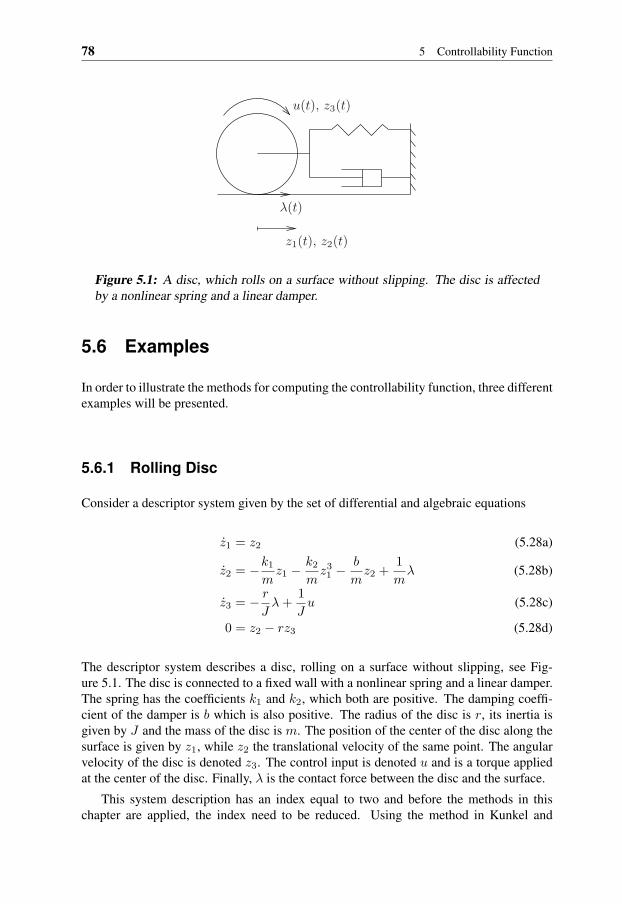
78 5 Controllability Function
u(t), z3(t)
λ(t)
z1(t), z2(t)
Figure 5.1: A disc, which rolls on a surface without slipping. The disc is affectedby a nonlinear spring and a linear damper.
5.6 Examples
In order to illustrate the methods for computing the controllability function, three differentexamples will be presented.
5.6.1 Rolling Disc
Consider a descriptor system given by the set of differential and algebraic equations
z1 = z2 (5.28a)
z2 = −k1
mz1 −
k2
mz31 −
b
mz2 +
1mλ (5.28b)
z3 = − rJλ+
1Ju (5.28c)
0 = z2 − rz3 (5.28d)
The descriptor system describes a disc, rolling on a surface without slipping, see Fig-ure 5.1. The disc is connected to a fixed wall with a nonlinear spring and a linear damper.The spring has the coefficients k1 and k2, which both are positive. The damping coeffi-cient of the damper is b which is also positive. The radius of the disc is r, its inertia isgiven by J and the mass of the disc is m. The position of the center of the disc along thesurface is given by z1, while z2 the translational velocity of the same point. The angularvelocity of the disc is denoted z3. The control input is denoted u and is a torque appliedat the center of the disc. Finally, λ is the contact force between the disc and the surface.
This system description has an index equal to two and before the methods in thischapter are applied, the index need to be reduced. Using the method in Kunkel and

5.6 Examples 79
Mehrmann (2001), (5.28) can be rewritten as the following index one description
z1 = z2 (5.29a)
z2 = −k1
mz1 −
k2
mz31 −
b
mz2 +
1mλ (5.29b)
0 = z2 − rz3 (5.29c)
0 = −k2
mz31 −
k1
mz1 −
b
mz2 +
(r2
J+
1m
)λ+
−rJu (5.29d)
We will use the abbreviation x = (z1, z2, z3, λ)T and it can be seen that x1 = (z1, z2)T
and x2 = (z3, λ)T .From (5.6d), it follows that W2 must satisfy
W2(x1, x2) = −Vx1(x1)F1;x2(x1, x2, u)F−12;x2
(x1, x2, u)
= −Vx1(x1)(
0 00 J
J+mr2
) (5.30)
Since F1 is independent of u, (5.6a) becomes
u = F2,u(x1, x2, u)TW2(x1, x2)T =(0 r
J+mr2
)Vx1(x1)T (5.31)
For (5.29), it is possible to compute x2 = ϕ(x1, u) explicitly using the last two rows as
z3 =1rz2
λ =(r2
J+
1m
)−1(k1
mz1 +
k2
mz31 +
b
mz2 +
r
Ju
) (5.32)
Inserting (5.31) and (5.32) into (5.6b) and letting V (x1) = a1z21 + a2z
41 + a3z
22 makes
it possible to solve (5.6b) for the unknowns a1, a2 and a3. The in this way obtainedsolutions for V (x1) become either
V (x1) = bk1r2z2
1 +12bk2r
2z41 + b
(J +mr2
)z22 (5.33)
or the trivial solution V (x1) = 0. Back-substitution of (5.33) into (5.30) and (5.31) yields
W2(x1, x2) =(0 −2bJz2
), u(x1) = 2brz2 (5.34)
The system is polynomial, and for given values of the parameters it would be possibleto use the method in (Ebenbauer and Allgöwer, 2004) to show asymptotic anti-stabilityof (5.29) with the control choice (5.34). Instead, stability is proven using the closed loopreduced system when the time is considered as going backwards, i.e.,
x1 = −Fred,cl(x1)
where
Fred,cl(x1) =
(z2
− k1Jr2 +m
z1 − k2Jr2 +m
z31 − b
Jr2 +m
z2 + 1( J
r2 +m)r2brz2
)

80 5 Controllability Function
For this system, V (x1) is a Lyapunov function since
V (x1) = bk1r2z2
1 +12bk2r
2z41 + b
(J +mr2
)z22 > 0
−Vx1(x1)Fred,cl(x1) = −2b2r2z22 < 0
for all x1 6= 0, since if the Vx1(x1)Fred,cl(x1) = 0 it requires that z2 = 0, but then z1 = 0because k1 and k2 being positive. Therefore, the conditions in Theorem 5.1 are fulfilled,yielding
Lc(x1) = V (x1)
for all x1 ∈ R2 with u(x1) chosen as (5.34).
5.6.2 Artificial System
The system in this section is completely artificial, but illustrates an advantage of the meth-ods in Sections 5.2 and 5.3.
The system dynamics are given by
z1 = −z1 + z2 +12z22
0 = z2 − u
where x1 = z1 and x2 = z2. This system fits into the control affine structure (5.9) orthe simplified structure (5.7) as well. The interesting feature is that the correspondingstate-space model
z1 = −z1 + u+12u2
is not control affine, and it would therefore not be possible to handle using the results inScherpen (1994). It can also be realized that the smallest reachable state is z1 = − 1
2 ,since u+ 1
2u2 > − 1
2 .Since the system fits into (5.7) the necessary conditions in Proposition 5.1 reduce to
the conditions (5.8) which in this case become
0 = W1(x1)(−z1 −12z22) +
12W1(x1)2(1 + z2)2 (5.35a)
0 = z2 − (1 + z2)W1(x1) (5.35b)
where we have used that
f(x1, x2) = −z1 + z2 +12z22 − (1 + z2)z2 = −z1 −
12z22
g(x1, x2) = 1 + z2
The equation for the control law is
u = (1 + z2)W1(x1)
and W2(x1, x2) is given by
W2(x1, x2) = −(1 + z2)W1(x1)
5.6 Examples 81
From (5.35b) it follows that
W1(x1) =z2
1 + z2
where it is assumed that z2 6= −1. Combining this equation with (5.35a) yields
0 =z2
(1 + z2)
(− z1 +
12z2
)which has the solutions
z2 = 0, z2 = 2z1
For the first solution, z2 = 0, the variables u, W1(x1) and W2(x1, x2) become
u = 0, W1(x1) = 0, W2(x1, x2) = 0
while the second solution, z2 = 2z1, gives
u = 2z1, W1(x1) =2z1
1 + 2z1, W2(x1, x2) = −2z1
Hence, two different solutions to the necessary conditions in Proposition 5.1 are ob-tained. Since the system has control-affine structure, Theorem 5.1 can be used to de-termine which of these solutions that is optimal. The first solution solves (5.10) onN = z1 ∈ R, z2 ∈ R | z2 = 0, while the second solution solves (5.10) on N =z1 ∈ R, z2 ∈ R | z1 > − 1
2 , z2 = 2z1. The solution with z1 < − 12 has been omitted,
since the set for z1 must contain the origin.For the first solution the closed loop dynamics are given by z1 = −z1, which is
asymptotically stable. Therefore, this solution cannot correspond to the controllabilityfunction.
For the second solution the closed loop system z1 = z1(1 + 2z1) is asymptoticallyanti-stable on N . Hence, this solution corresponds to the controllability function, whichin this case for z1 > − 1
2 becomes
Lc(x1) = z1 −12
ln(2z1 + 1) (5.36)
In Figure 5.2, the controllability function is plotted. As can be seen the energy for reach-ing states close to z1 = − 1
2 goes towards infinity, which agrees with the discussion earlier.
5.6.3 Electrical Circuit
Finally, a small example is presented where the method in Section 5.4.2 is used. Thestudied process is the electrical circuit in Figure 5.3. The circuit consists of a voltagesource, a resistor, a capacitor and an inductor. The voltage source is assumed to be ideal,i.e., having no internal resistance and giving the voltage u. The inductor is assumed tohave a ferromagnetic core resulting in a saturated magnetic flux Φ for large currents i.

82 5 Controllability Function
z1
32.521.510.50
2
-0.5
1.5
1
0.5
0
Figure 5.2: The controllability function L(x1) for the artifical example.
u(t) L
R Ci(t)
uC(t)
uL(t)
uR(t)
Figure 5.3: An electrical circuit consisting of an ideal voltage source and threenonlinear components, namely a resistor, a capacitor and an inductor.

5.6 Examples 83
By modifying a general inductor model from Hasler and Neirynck (1986), the inductor ismodeled as
Φ = uL
Φ = arctan(i)
where uL is the voltage over the inductor. The capacitor is assumed to have a voltagedependent capacitance C and is therefore modeled as
(1 + 10−2uC)uC = i
where uC is the voltage over the capacitance. Finally, the resistor is described by
uR = i+ i3
where uR is the voltage over the resistor. That is, it is assume that uR except for a lineardependence of the current, also depend on the cube of the current.
If the notation z1 = uC , z2 = Φ, z3 = i and z4 = uL is used, a model for thecomplete system is
z1 =z3
1 + 10−2z1(5.37a)
z2 = z4 (5.37b)0 = z2 − arctan(z3) (5.37c)
0 = −z1 − z3 − z33 − z4 + u (5.37d)
where the last equation comes from Kirschoff’s voltage law. The model (5.37) is a de-scriptor system where x1 = (z1, z2)T and x2 = (z3, z4)T .
It can be verified that (5.37) satisfies Assumption A4, since
F2;x2(0, 0, 0) =(−1 0−1 −1
)The functions in (5.37) are analytical for z1 > −100 and Assumption A5 is therefore alsosatisfied. The series expansion of the implicit function up to order four becomes
ϕ(z1, z2, u) ≈(
z2 + 13z
32
−z1 − z2 − 43z
32 + u
)(5.38)
The matrices A and B can then be computed as
A =(
0 1−1 −1
), B =
(01
)and it can verified that A is Hurwitz and (A, B) is controllable. Theorem 5.2 now guar-antees the existence of a local controllability function (5.13) and a corresponding controlsignal (5.14).
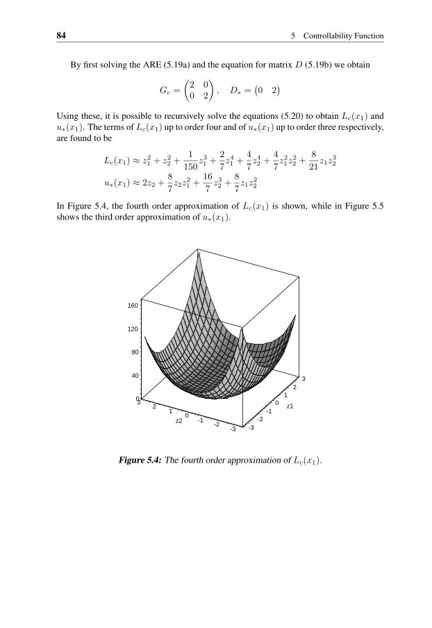
84 5 Controllability Function
By first solving the ARE (5.19a) and the equation for matrix D (5.19b) we obtain
Gc =(
2 00 2
), D∗ =
(0 2
)Using these, it is possible to recursively solve the equations (5.20) to obtain Lc(x1) andu∗(x1). The terms of Lc(x1) up to order four and of u∗(x1) up to order three respectively,are found to be
Lc(x1) ≈ z21 + z2
2 +1
150z31 +
27z41 +
47z42 +
47z21z
22 +
821z1z
32
u∗(x1) ≈ 2z2 +87z2z
21 +
167z32 +
87z1z
22
In Figure 5.4, the fourth order approximation of Lc(x1) is shown, while in Figure 5.5shows the third order approximation of u∗(x1).
32
103 0 z12
40
-110
80
-2-1z2
120
-2 -3-3
160
Figure 5.4: The fourth order approximation of Lc(x1).

5.6 Examples 85
32
13 0
-100
z12
-50
-110
0
-2-1z2
50
-2 -3-3
100
Figure 5.5: The third order approximation of u∗(x1).

86 5 Controllability Function
6Observability Function
In the previous chapter, the controllability function was investigated and some differentmethods to compute it were derived. In this chapter, the observability function is consid-ered instead. The observability function measures the energy in the output signal whenthe system is released from a given state and the control input is equal to zero. The basicidea is that if a state is observable, the energy in the output signal will be nonzero.
For nonlinear state-space systems in control-affine form, the computation of the ob-servability function has been studied in for example (Scherpen, 1994; Gray and Mesko,1999). Both these references also show that for a time-invariant linear state-space system,the observability function equals the observability gramian post- and pre-multiplied bythe state. To find the observability function, a linear partial differential equation needsto be solved. In practice, an explicit solution can be hard to find. Therefore, numeri-cal methods to compute the observability function have been studied. One such methodis described in Scherpen (1994) and yields a local observability function expressed as apower series. The computations are very similar to the computations in Chapter 4. An-other kind of methods are the empirical methods, based on stochastics, see Newman andKrishnaprasad (1998, 2000).
The observability function has also been studied for regular linear time-invariant de-scriptor systems with consistent initial conditions, see Stykel (2004). The method pre-sented by Stykel can also handle descriptor systems of higher index without using indexreduction.
In this chapter two different methods to calculate the observability function for non-linear descriptor systems are presented. In Section 6.2, the approach based on the explicitsolution of the first order linear partial differential equation is extended. As earlier men-tioned, it can in many cases be hard to find an explicit solution, and therefore the approachbased on power series is also extended. It means that a local observability function, validonly in a neighborhood of the origin, is found by recursive solution of the linear partialdifferential equation from Section 6.2.
87
88 6 Observability Function
6.1 Problem Formulation
The observability function should reflect the energy in the output signal when the systemis released from a certain initial state. It is only the energy corresponding to the initialstate that is of interest and and therefore the control signal is set to zero. The observabilityfunction Lo(x1) is then defined as
Lo
(x1(0)
)=
12
∞∫0
y(t)T y(t) dt (6.1)
subject to
x1(0) = x1,0 ∈ Ωx
u(t) = 0, 0 ≤ t <∞
and a descriptor system. In this chapter, the descriptor system is assumed to be in theform
x1 = F1(x1, x2) (6.2a)0 = F2(x1, x2) (6.2b)y = h(x1, x2) (6.2c)
Hence, an output equation is added explicitly and it is assumed that h(0, 0) = 0. Thedescriptor system (6.2) is also assumed to have an equilibrium at the origin.
Similar to Chapter 5, different assumptions on the implicit function is used in thedifferent sections. In Section 6.2, Assumption A2 is made while in Section 6.3, As-sumption A4 is used instead. In both cases, it is known that on a set Ωx, it holds thatx2 = ϕ(x1). The corresponding set of points (x1, x2) satisfying the constraints will bedenoted N , i.e.,
N = x1 ∈ Ωx, x2 ∈ Rn2 |x2 = ϕ(x1) (6.3)
Throughout this chapter, it is assumed that x2(0) = x2,0 is chosen such that (x1,0, x2,0) ∈N , i.e., only consistent initial values are considered.
Since the control input cannot be used to stabilize the system, it is also necessary that(6.2) is asymptotically stable, at least locally on some set Ω′
x ⊂ Ωx around the origin.Otherwise, Lo(x1,0) might become infinite. For notational convenience the consistentstates corresponding to Ω′
x is defined as
N ′ = x1 ∈ Ω′x, x2 ∈ Rn2 |x2 = ϕ(x1)
A boundary condition for the observability function is Lo(0) = 0, since the origin isan equilibrium and h(0, 0) = 0.
A small but perhaps clarifying note is that in contrast to the controllability functioncomputation, the observability function computation does not include optimization. It isjust a matter of finding the solution to the system, i.e., x(t), for a given initial conditionand then integrating the square of the corresponding output.
Remark 6.1. As in the controllability function case it is possible to consider more generalenergy measures. That is, instead of using 1
2y(t)T y(t) in (6.1), the energy measure can
be some positive definite function m(y(t)
).
6.2 Method Based on Partial Differential Equation 89
6.2 Method Based on Partial Differential Equation
Solving the descriptor system (6.2) in order to obtain an explicit solution for y(t), whichcan be squared and integrated, is typically very hard. Therefore, other methods need tobe derived.
One such method is based on a first-order linear partial differential equation. Themethod is presented in the following theorem and is an extension of a result in Scherpen(1994).
Theorem 6.1Suppose the system (6.2) is asymptotically stable for x1,0 ∈ Ω′
x. Further, assume there ex-ists a continuously differentiable positive semidefinite function V (x1) satisfying V (0) = 0and
0 =12h(x1, x2)Th(x1, x2) + Vx1(x1)F1(x1, x2) (6.4)
for all (x1, x2) ∈ N ′. Then for all x1,0 ∈ Ω′x, it holds that
Lo(x1,0) = V (x1,0) (6.5)
Proof: Assume that only x1,0 ∈ Ω′x are considered. Then, for any solution to (6.2) it
follows that
V(x1(0)
)=
∞∫0
dV(x(t)
)dt
dt =
∞∫0
−Vx1F1 dt =
∞∫0
yT y dt (6.6)
provided (6.4) is satisfied and V (x1) is a sufficiently smooth function. Therefore, for allx1,0 ∈ Ω′
x it follows that
Lo(x1,0) =12
∞∫0
yT y dt = V (x1,0)
The setN ′ defines, in a rather implicit manner, that (6.4) only needs to be satisfied for(x1, x2) satisfying the constraint equation. However, this dependence can be expressedmore explicitly by including the constraint equation as part of the condition as well. Then,the condition (6.4) can be reformulated as
0 =12h(x1, x2)Th(x1, x2) + Vx1(x1)F1(x1, x2)
0 = F2(x1, x2)
which must hold for x1 ∈ Ω′x. Another reformulation is to use that for (x1, x2) ∈ N ′ it
is known that x2 = ϕ(x1) and the result then becomes
0 =12h(x1, ϕ(x1)
)Th(x1, ϕ(x1)
)+ Vx1(x1)F1
(x1, ϕ(x1)
)(6.7)
which must hold for x1 ∈ Ω′x. The last equation clearly shows that the implicit function
must be known explicitly to compute the observability function in this way. This is amajor drawback for many systems.

90 6 Observability Function
6.3 Method to Find a Local Solution
In earlier chapters, it has been shown that one method to overcome the problem of notknowing an explicit expression for the implicit function ϕ(x1) is to solve the problemslocally in some neighborhood of the origin. In that case, a power series expansion of theimplicit function is enough and if certain assumptions are made, it is well-known thatsuch a power series can be calculated. In this section these assumptions are formulated,and a local observability function valid in an neighborhood of the origin, is derived.
6.3.1 Basic Assumptions and Calculation of the Power Series Ex-pansion of the Reduced System
Consider descriptor systems (6.2) which satisfies Assumption A4. Similar to in Chapter 4,another assumption is also made.
Assumption A7. The functions F1, F2 and h are analytical on a set W defined as
W = x1 ∈ Wx1 ⊂ Ωx, x2 ∈ Wx2 ⊃ ϕ(Wx1) (6.8)
where Wx1 and Wx2 are neighborhoods of x1 = 0 and x2 = 0, respectively.
Here, Ωx is the neighborhood on which the implicit function is defined. Based onAssumption A7 it follows that F1, F2 and h in (6.2) can be expanded in convergent powerseries as (
F1(x1, x2)F2(x1, x2)
)=(A11 A12
A21 A22
)(x1
x2
)+(F1h(x1, x2)F2h(x1, x2)
)h(x1, x2) =
(C1 C2
)(x1
x2
)+ hh(x1, x2)
where Fih(x1, x2) for i = 1, 2 and hh(x1, x2) contains higher order terms of at leastdegree two. From Assumption A4 it is known that A22 has full rank, since F2;x2(0, 0) =A22 is nonsingular.
The system (6.2) can be written as the reduced state-space system
x1 = F1(x1) = F1
(x1, ϕ(x1)
)y = h(x1) = h
(x1, ϕ(x1)
)and by making a series expansion of the implicit function ϕ(x1) using the method inSection 4.3.1, the power series expansions of the composite functions F1 and h can beexpressed as
F1(x1) = Ax1 + F1h(x1), h(x1) = Cx1 + hh(x1) (6.9)
where
A = A11 −A12A−122 A21, C = C1 − C2A
−122 A21
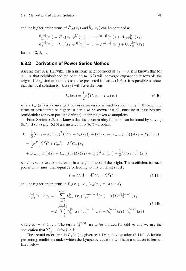
6.3 Method to Find a Local Solution 91
and the higher order terms of F1h(x1) and hh(x1) can be obtained as
F[m]1h (x1) = F1h
(x1, ϕ
[1](x1) + . . . ϕ[m−1](x1))
+A12ϕ[m]h (x1)
h[m]h (x1) = h1h
(x1, ϕ
[1](x1) + . . .+ ϕ[m−1](x1))
+ C2ϕ[m]h (x1)
for m = 2, 3, . . ..
6.3.2 Derivation of Power Series Method
Assume that A is Hurwitz. Then in some neighborhood of x1 = 0, it is known that forx1,0 in that neighborhood the solution to (6.2) will converge exponentially towards theorigin. Using similar methods to those presented in Lukes (1969), it is possible to showthat the local solution for Lo(x1) will have the form
Lo(x1) =12xT
1 Gox1 + Loh(x1) (6.10)
where Loh(x1) is a convergent power series on some neighborhood of x1 = 0 containingterms of order three or higher. It can also be shown that Go must be at least positivesemidefinite (or even positive definite) under the given assumptions.
From Section 6.2, it is known that the observability function can be found by solving(6.7). If (6.9) and (6.10) are inserted into (6.7) we obtain
0 =12(Cx1 + hh(x1)
)T (Cx1 + hh(x1)
)+(xT
1 Go + Loh;x1(x1))(Ax1 + F1h(x1)
)=
12xT
1
(CT C +GoA+ ATGo
)x1
+ Loh;x1(x1)Ax1 + Lo;x1(x1)Fh(x1) + xT1 C
T hh(x1) +12hh(x1)T hh(x1)
which is supposed to hold for x1 in a neighborhood of the origin. The coefficient for eachpower of x1 must then equal zero, leading to that Go must satisfy
0 = GoA+ ATGo + CT C (6.11a)
and the higher order terms in Lo(x1), i.e., Loh(x1) must satisfy
L[m]o;x1
(x1)Ax1 = −m−1∑k=2
L[k]o;x1
(x1)F[m+1−k]1h (x1)− xT
1 CT h
[m−1]h (x1)
− 2bm−1
2 c∑k=2
h[k]h (x1)T h
[m−k]h (x1)− h
[m/2]h (x1)T h
[m/2]h (x1)
(6.11b)
where m = 3, 4, . . .. The terms h[m/2]h are to be omitted for odd m and we use the
convention that∑l
k = 0 for l < k.The second order term in Lo(x1) is given by a Lyapunov equation (6.11a). A lemma
presenting conditions under which the Lyapunov equation will have a solution is formu-lated below.
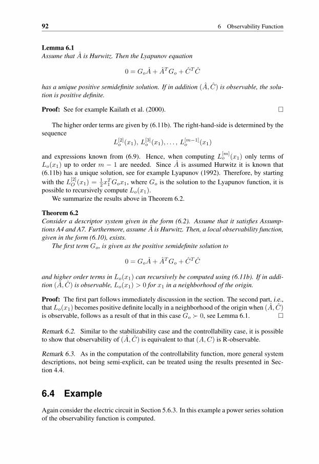
92 6 Observability Function
Lemma 6.1Assume that A is Hurwitz. Then the Lyapunov equation
0 = GoA+ ATGo + CT C
has a unique positive semidefinite solution. If in addition (A, C) is observable, the solu-tion is positive definite.
Proof: See for example Kailath et al. (2000).
The higher order terms are given by (6.11b). The right-hand-side is determined by thesequence
L[2]o (x1), L[3]
o (x1), . . . , L[m−1]o (x1)
and expressions known from (6.9). Hence, when computing L[m]o (x1) only terms of
Lo(x1) up to order m − 1 are needed. Since A is assumed Hurwitz it is known that(6.11b) has a unique solution, see for example Lyapunov (1992). Therefore, by startingwith the L[2]
O (x1) = 12x
T1 Gox1, where Go is the solution to the Lyapunov function, it is
possible to recursively compute Lo(x1).We summarize the results above in Theorem 6.2.
Theorem 6.2Consider a descriptor system given in the form (6.2). Assume that it satisfies Assump-tions A4 and A7. Furthermore, assume A is Hurwitz. Then, a local observability function,given in the form (6.10), exists.
The first term Go, is given as the positive semidefinite solution to
0 = GoA+ ATGo + CT C
and higher order terms in Lo(x1) can recursively be computed using (6.11b). If in addi-tion (A, C) is observable, Lo(x1) > 0 for x1 in a neighborhood of the origin.
Proof: The first part follows immediately discussion in the section. The second part, i.e.,thatLo(x1) becomes positive definite locally in a neighborhood of the origin when (A, C)is observable, follows as a result of that in this case Go 0, see Lemma 6.1.
Remark 6.2. Similar to the stabilizability case and the controllability case, it is possibleto show that observability of (A, C) is equivalent to that (A,C) is R-observable.
Remark 6.3. As in the computation of the controllability function, more general systemdescriptions, not being semi-explicit, can be treated using the results presented in Sec-tion 4.4.
6.4 Example
Again consider the electric circuit in Section 5.6.3. In this example a power series solutionof the observability function is computed.
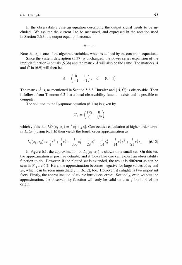
6.4 Example 93
In the observability case an equation describing the output signal needs to be in-cluded. We assume the current i to be measured, and expressed in the notation usedin Section 5.6.3, the output equation becomes
y = z3
Note that z3 is one of the algebraic variables, which is defined by the constraint equations.Since the system description (5.37) is unchanged, the power series expansion of the
implicit function ϕ equals (5.38) and the matrix A will also be the same. The matrices Aand C in (6.9) will then be
A =(
0 1−1 −1
), C =
(0 1
)The matrix A is, as mentioned in Section 5.6.3, Hurwitz and (A, C) is observable. Thenit follows from Theorem 6.2 that a local observability function exists and is possible tocompute.
The solution to the Lyapunov equation (6.11a) is given by
Go =(
1/2 00 1/2
)which yields thatL[2]
o (z1, z2) = 14z
21+ 1
4z22 . Consecutive calculation of higher order terms
in Lo(x1) using (6.11b) then yields the fourth order approximation as
Lo(z1, z2) ≈14z21 +
14z22 +
1600
z31 −
128z41 −
114z42 −
114z22z
21 +
121z32z1 (6.12)
In Figure 6.1, the approximation of Lo(z1, z2) is shown on a small set. On this set,the approximation is positive definite, and it looks like one can expect an observabilityfunction to do. However, if the plotted set is extended, the result is different as can beseen in Figure 6.2. Here, the approximation becomes negative for large values of z1 andz2, which can be seen immediately in (6.12), too. However, it enlightens two importantfacts. Firstly, the approximation of course introduces errors. Secondly, even without theapproximation, the observability function will only be valid on a neighborhood of theorigin.
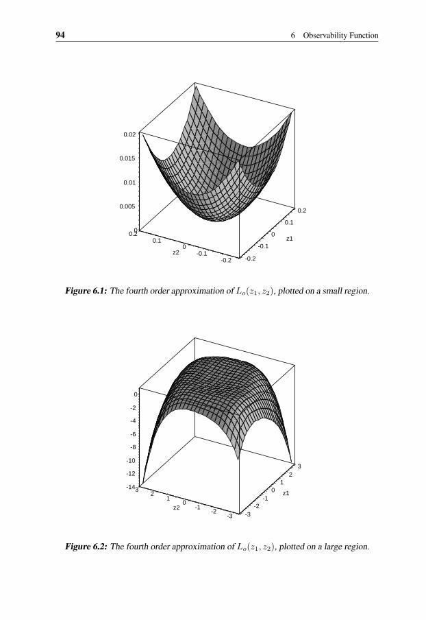
94 6 Observability Function
0.2
0.10
0.2 0z10.1
0.005
-0.10
0.01
z2 -0.1
0.015
-0.2-0.2
0.02
Figure 6.1: The fourth order approximation of Lo(z1, z2), plotted on a small region.
32
1-143 0
-12
z12
-10
-11
-8
0
-6
-2-1z2
-4
-2 -3
-2
-3
0
Figure 6.2: The fourth order approximation of Lo(z1, z2), plotted on a large region.

7Concluding Remarks
In this chapter we present some conclusions and some possible research openings foundduring the work.
7.1 Conclusions
In this thesis we have mainly studied optimal feedback control and computation of thecontrollability function and observability function, respectively. The methods presentedfor solving these problems can be divided into two groups, namely those needing anexplicit expression for the implicit function and those that only need its power seriesexpansion.
Unfortunately for the first group, an explicit expression for the implicit function isknown only for certain classes of systems. Moreover, even when the implicit function canbe expressed explicitly the solution of the nonlinear partial differential equation obtainedin the optimal control problems has to be found. Therefore, this kind of methods havelimited usability in real life applications.
The methods based on power series expansions do not suffer from these problems, andcan rather easily be computed for moderately sized nonlinear descriptor systems using asymbolic tool such as Maple or MATHEMATICA. It has been showed how in principle thealgorithm presented in Chapter 4 can be applied to an index reduced descriptor systemalmost without any reformulations or assumptions. This fact opens a lot of possibilities.A possible drawback is that the computed feedback law is optimal only locally. However,in many applications a local reult can be enough. Another drawback with methods basedon power series expansions is the possible difficulty to know in which region the solutionactually is optimal.
95
96 7 Concluding Remarks
7.2 Future work
There are a lot of possible research openings related to the work in this thesis. Most ofthe them are associated with the power series expansion method described in Chapter 4.The reason is the lack of an explicit expression for the implicit function which most oftenis a complicating fact. However, a few interesting questions can also be found in the casewhen an explicit expression is required. One such question is which conditions W2 inSection 3.2 must satisfy in cases when the descriptor system does not satisfy Assump-tion A2. The answer would probably increase the usability of the theorem in Xu andMizukami (1993).
For the power series method there are numerous extensions. For example, it would beinteresting to extend the power series method in Chapter 4 to handle discrete-time descrip-tor systems and performance criterions with finite time-horizon as well. Another possibledevelopment could be to extend the method for computation of a Lyapunov function usingseries expansion. A third interesting extension would be to find the power series solutionof the optimal feedback control problem without assuming that the system satisfies As-sumption A4. In this case, one further requirement on the controller is to make the closedloop system index one.
A problem with the methods based on power series expansions is that it can often bedifficult to determine in what region the optimal solution is obtained. For state-space sys-tems other methods to find approximative optimal solutions exist, for example where theHJB is approximated using succesive Galerkin approximations etc. It would be interestingto study if these methods can be extended to handle descriptor systems as well.
In the area of controllability and observability it would be nice to extend the notionof the natural observability function appearing in (Gray and Mesko, 1999; Scherpen andGray, 2000). It is defined similarly to the ordinary observability function but also includesa maximization.
The reason for Scherpen and Gray to study the controllability function and observabil-ity function in the state-space case are model reduction. For linear time-invariant systemsthe extension to descriptor systems is already done, but perhaps also nonlinear descriptorsystems can be handled.
Finally, it would be interesting to try some of the methods in real life applications.
ASome Facts from Calculus and Set
Theory
This appendix provides the reader with simple definitions of some frequently used resultsfrom mathematics. For more rigorous mathematical definitions of the different conceptsthe reader is referred to (Isidori, 1995; Khalil, 2002) and references therein.
Manifolds
A k-dimensional manifold in Rn can be thought of as the solution of the equation
η(x) = 0
where η : Rn → Rn−k is sufficiently smooth, i.e., sufficiently many times continuouslydifferentiable. A small example of a manifold is the n-dimensional unit sphere
x ∈ Rn |
n∑i=1
x2i = 1
which is a (n− 1)-dimensional manifold in Rn.
Sets
Two topological concepts frequently used in this thesis are neighborhoods and balls. Aneighborhood of a point p is any open set which contains p. A ball Bδ is an open setaround some point p with radius δ, i.e.,
Bδ = x ∈ Rn | ‖x− p‖ < δ, 0 < δ
where the norm can be any norm, but in this thesis always the Euclidian norm, i.e., ‖x‖ =√xTx, will be used. Since a neighborhood is an open set, it is always possible to place
97
98 A Some Facts from Calculus and Set Theory
a ball inside it and vice versa. It is therefore common that neighborhoods are assumed tobe balls.
In many cases, such as in the stability analysis, the considered sets are assumed openand connected. A set is connected if every pair of points in the set can be joined by an arclying in the set.
Rank of Matrix-Valued Functions
The rank of a matrix-valued function F : Rn → Rm at x0 ∈ Rn, is the rank of the matrixobtained if F is evaluated at x0. Sometimes the rank of F on a manifold is considered.The rank of F is then evaluated pointwise for all points belonging to the manifold.
The corank of a matrix-valued function F in x0 is the rank deficiency of F (x) withrespect to rows. That is, it is the rank of the corange, which is the nullspace of F (x)T .These concepts can be studied on a manifold as well. A small example is the function
F (x1, x2) =
x1 00 x2
x21 x2
2
which at (x0
1, x02) = (1, 0) has rank one and corank two, while for (x0
1, x02) = (1, 1) has
rank two and corank one.
Implicit Function Theorem
One of the most used theorems in this thesis is the implicit function theorem, Theo-rem A.1.
Theorem A.1Let F : Cm × Cn → Cm be an analytic function of (x, y) in a neighborhood of a point(x0, y0). Assume that F (x0, y0) = 0 and that the matrix Fx(x0, y0) is nonsingular. Then,the equation F (x, y) = 0 has a uniquely determined analytic solution
x = ϕ(y)
in a neighborhood of y0, such that ϕ(y0)
= x0.
Proof: See Hörmander (1966).
If F is k-times continuously differentiable instead, the implicit function ϕ is k-timescontinuously differentiable as well. The function ϕ is often called a diffeomorphism. Itmeans that ϕ is a continuously differentiable function between manifolds, with a continu-ously differentiable inverse. However, in some references the continuous differentiabilityis strengthened to C∞.
Bibliography
Al’brekht, E. G. (1961). On the optimal stabilization of nonlinear systems. Journal ofApplied Mathematics and Mechanics, 25(5):1254–1266.
Arnold, M., Mehrmann, V., and Steinbrecher, A. (2004). Index reduction in industrialmultibody system simulation.
Ascher, U. M., Hongsheng, C., and Reich, S. (1994). Stabilization of DAE’s and invariantmanifolds. Numerische Mathematik, 67(2):131–149.
Bardi, M. and Capuzzo-Dolcetta, I. (1997). Optimal Control and Viscosity Solutionsof Hamilton-Jacobi-Bellman Equations. Systems & Control: Foundations & Applica-tions. Birkhäuser, Boston.
Baumgarte, J. (1972). Stabilization of constraints and integrals of motion in dynamicalsystems. Computer Methods in Applied Mechanics and Engineering, 1:1–16.
Beard, R. W., Saridis, G. N., and Wen, J. T. (1998). Approximative solutions to thetime-invariant Hamilton-Jacobi-Bellman equation. Journal of Optimization Theory andApplications, 96(3):589–626.
Bellman, R. E. (1957). Dynamic Programming. Princeton University Press, New Jersey.
Bender, D. J. and Laub, A. J. (1987). The linear-quadratic optimal regulator for descriptorsystems. IEEE Transactions on Automatic Control, AC-32(8):672–688.
Bertsekas, D. P. (1995). Dynamic Programming and Optimal Control, volume 1. AthenaScientific, Belmont, USA.
Bittanti, S., Laub, A. J., and Willems, J. C., editors (1991). The Riccati Equation. Com-munications and Control Engineering. Springer-Verlag, Berlin.
99

100 Bibliography
Brenan, K. E., Campbell, S., and Petzold, L. R. (1996). Numerical Solution of Initial-Value Problems in Differential-Algebraic Equations. SIAM, New York.
Brown, J. W. and Churchill, R. V. (1996). Complex Variables and Applications. McGraw-Hill, New York, 6th edition.
Bryson, A. E. and Ho, Y.-C. (1975). Applied Optimal Control — Optimization, Estima-tion and Control. Hemisphere Pub. Corp., Washington. rev. pr.
Campbell, S. L. (1995). Linearization of DAE’s along trajectories. Zeitschrift für ange-wandte Mathematik und Physik, 46(1):70–84.
Campbell, S. L. and Gear, C. W. (1995). The index of general nonlinear DAEs. Nu-merische Mathematik, 72:173–196.
Campbell, S. L. and Griepentrog, E. (1995). Solvability of general differential algebraicequations. SIAM Journal on Scientific Computing, 16(2):257–270.
Campbell, S. L., Kelley, C. T., and Yeomans, K. D. (1996). Consistent initial condi-tions for unstructured higher index DAEs: A computational study. In Proceedings ofComputational Engineering in Systems Applications, pages 416–421, Lille, France.
Cebuhar, W. A. and Costanza, V. (1984). Approximation procedures for the optimalcontrol of bilinear and nonlinear systems. Journal of Optimization Theory and Appli-cations, 43(4):615–627.
Cobb, J. D. (1980). Descriptor Variable and Generalized Singularly Perturbed Systems:A Geometric Approach. PhD thesis, University of Illinois, Urbana, Illinois.
Cobb, J. D. (1983). Descriptor variable systems and optimal state regulation. IEEETransactions on Automatic Control, AC-28(5):601–611.
Dai, L. (1989). Singular Control Systems. Lecture Notes in Control and InformationSciences. Springer-Verlag, Berlin.
Ebenbauer, C. and Allgöwer, F. (2004). Computer-aided stability analysis of differential-algebraic equations. In Proceedings of the 6th Symposium on Nonlinear Control Sys-tems, pages 1025–1029, Stuttgart, Germany.
Gerdin, M. (2004). Parameter estimation in linear descriptor systems. Technical ReportLicentiate Thesis no. 1085, Department of Electrical Engineering, Linköpings univer-sitet, SE-581 83 Linköping, Sweden.
Glad, T. and Sjöberg, J. (2005). Optimal control for nonlinear descriptor systems. Techni-cal Report LiTH-ISY-R-2702, Department of Electrical Engineering, Linköpings uni-versitet.
Gray, W. S. and Mesko, J. P. (1999). Observability functions for linear and nonlinearsystems. Systems & Control Letters, 38(2):99–113.
Hahn, H. (2002). Rigid Body Dynamics of Mechanics 1 — Theoretical Basis. Springer-Verlag, Berlin.

Bibliography 101
Hahn, H. (2003). Rigid Body Dynamics of Mechanics 2 — Applications. Springer-Verlag, Berlin.
Hasler, M. and Neirynck, J. (1986). Nonlinear Circuits. Artech House, Norwood.
Hill, D. J. and Mareels, I. M. Y. (1990). Stability theory for differential algebraic sys-tems with application to power systems. IEEE Transactions on Circuits and Systems,37(11):1416–1423.
Hörmander, L. (1966). An Introduction to Complex Analysis in Several Variables. TheUniversity Series in Higher Mathematics. D. Van Nostrand, Princeton, New Jersey.
Isaacs, R. (1965). Differential games : a mathematical theory with applications to warfareand pursuit, control and optimization. Wiley, New York.
Isidori, A. (1995). Nonlinear Control Systems. Springer-Verlag, London, 3rd edition.
Jonckheere, E. A. (1988). Variational calculus for descriptor systems. IEEE Transactionson Automatic Control, AC-33(5):491–495.
Jönsson, U., Trygger, C., and Ögren, P. (2002). Lectures in optimal control. KungligaTekniska högskolan, Stockholm.
Kailath, T., Sayed, A. H., and Hassibi, B. (2000). Linear Estimation. Prentice Hall, UpperSaddle River, New Jersey.
Kalman, R. E. (1963). The theory of optimal control and the calculus of variations. InBellman, R., editor, Mathematical optimization techniques, pages 309–331. Universityof California Press, Berkeley, California.
Khalil, H. K. (2002). Nonlinear Systems. Prentice Hall, Upper Saddle River, New Jersey,3rd edition.
Krener, A. J. (1992). The construction of optimal linear and nonlinear regulators. InIsidori, A. and Tarn, T. J., editors, Systems, Models and Feedback: Theory and Appli-cations, pages 301–322. Birkhäuser, Boston.
Krener, A. J. (2001). The local solvability of a Hamilton-Jacobi-Bellman PDE around anonhyperbolic critical point. SIAM Journal on Control and Optimization, 39(5):1461–1484.
Kumar, A. and Daoutidis, P. (1999). Control of nonlinear differential algebraic equationsystems. Chapman & Hall CRC.
Kunkel, P. and Mehrmann, V. (1994). Canonical forms for linear differential-algebraicequations with variable coefficients. Journal of Computational and Applied Mathemat-ics, 56(3):225–251.
Kunkel, P. and Mehrmann, V. (1996). Local and global invariants of linear differential-algebraic equations and their relation. Electronic Transactions on Numerical Analysis,4:138–157.
102 Bibliography
Kunkel, P. and Mehrmann, V. (1998). Regular solutions of nonlinear differential-algebraicequations and their numerical determination. Numerische Mathematik, 79:581–600.
Kunkel, P. and Mehrmann, V. (2001). Analysis of over- and underdetermined nonlineardifferential-algebraic systems with application to nonlinear control problems. Mathe-matics of Control, Signals, and Systems, 14:233–256.
Kunkel, P. and Mehrmann, V. (2004). Index reduction for differential-algebraic equa-tions by minimal extension. Zeitschrift für Angewandte Mathematik und Mechanik,84(9):579–597.
Lee, E. B. and Markus, L. (1967). Foundations of Optimal Control Theory. Wiley, NewYork.
Leitmann, G. (1981). The Calculus of Variations and Optimal Control. Plenum Press,New York.
Lin, J.-Y. and Ahmed, N. U. (1991). Approach to controllability problems for singularsystems. International Journal of Systems Science, 22(4):675–690.
Luenberger, D. G. (1978). Time-invariant descriptor systems. Automatica, 14(5):473–480.
Lukes, D. L. (1968). Stabilizability and optimal control. Funkcialaj Ekvacioj, 11(1):39–50.
Lukes, D. L. (1969). Optimal regulation of nonlinear dynamical systems. SIAM Journalon Control, 7(1):75–100.
Lyapunov, A. M. (1992). The General Problem of the Stability of Motion. Taylor andFrancis, London.
Mahony, R. E. and Mareels, I. M. (1995). Global solutions for differential/algebraic sys-tems and implications for Lyapunov direct stability methods. Journal of MathematicalSystems, Estimation, and Control, 5(4):1–26.
Mattson, S. E. and Söderlind, G. (1993). Index reduction in differential-algebraic equa-tions using dummy derivatives. SIAM Journal on Scientific Computing, 14(3):677–692.
McClamroch, N. H. (1990). Feedback stabilization of control systems described by a classof nonlinear differential-algebraic equations. Systems & Control Letters, 15(1):53–60.
Mehrmann, V. (1989). Existence, uniqueness, and stability of solutions to singular linearquadratic optimal control problems. Linear Algebra and Its Applications, 121:291–331.
Navasca, C. L. (1996). Local Solutions of the Dynamic Programming Equations and theHamilton Jacobi Bellman PDE. PhD thesis, University of California, Davis.
Navasca, C. L. and Krener, A. J. (2000). Solution of Hamilton-Jacobi-Bellman equations.In Proceedings of the 39th IEEE Conference on Decision and Control, pages 570–574,Sydney, Australia.
Bibliography 103
Newman, A. J. and Krishnaprasad, P. S. (1998). Computation for nonlinear balancing. InProceedings of the 37th IEEE Conference on Decision and Control, pages 4103–4104,Tampa, Florida.
Newman, A. J. and Krishnaprasad, P. S. (2000). Computing balanced realizations fornonlinear systems. In Fourteenth International Symposium on Mathematical Theory ofNetworks and Systems, Perpignan, France.
Pantelides, C. (1988). The consistent initialization of differential-algebraic systems.SIAM Journal on Scientific Computing, 9(2):213 – 231.
Pesch, H. J. and Bulirsch, R. (1994). The Maximum Principle, Belmann’s Equation andCarathéodory’s work. Journal of Optimization Theory and Applications, 80(2):199–225.
Polderman, J. W. and Willems, J. C. (1998). Introduction to mathematical systems theory:a behavioral approach. Springer-Verlag, New York.
Rheinboldt, W. and Simeon, B. (1999). On computing smooth solutions of DAEs forelastic multibody systems. Computers & Mathematics with Applications, 37(6):69–83.
Rouchon, P., Fliess, M., and Lévine, J. (1992). Kronecker’s canonical form for nonlinearimplicit differential systems. In 2nd IFAC Workshop on System Structure and Control,Prague, Czech Republic.
Scherpen, J. M. A. (1994). Balancing for Nonlinear Systems. PhD thesis, University ofTwente, The Netherlands.
Scherpen, J. M. A. and Gray, W. S. (2000). Minimality and local state decompositionsof a nonlinear state space realization using energy functions. IEEE Transactions onAutomatic Control, AC-45(11):2079–2086.
Simeon, B., Grupp, F., Führer, C., and Rentrop, P. (1994). A nonlinear truck model and itstreatment as a multibody system. Journal of Computational and Applied Mathematics,50:523–532.
Sjöberg, J. (2005). Descriptor systems and control theory. Technical Report LiTH-ISY-R-2688, Department of Electrical Engineering, Linköpings universitet, SE-581 83Linköping, Sweden.
Sjöberg, J. and Glad, T. (2005a). Computing the controllability function for nonlineardescriptor systems. Technical Report LiTH-ISY-R-2717, Department of Electrical En-gineering, Linköpings universitet, SE-581 83 Linköping, Sweden.
Sjöberg, J. and Glad, T. (2005b). Power series solution of the Hamilton-Jacobi-Bellmanequation for descriptor systems. In Proceedings of the 44th IEEE Conference on Deci-sion and Control, Seville, Spain.
Stykel, T. (2004). Gramian-based model reduction for descriptor systems. Mathematicsof Control, Signals, and Systems, 16:297–319.

104 Bibliography
Sussmann, J., H. and Willems, C., J. (1997). 300 years of optimal control: Fromthe brachystochrone to the maximum principle. IEEE Control Systems Magazine,17(3):32–44.
Tischendorf, C. (2003). Coupled systems of differential algebraic and partial differentialequations in circuit and device simulation – modeling and numerical analysis. Habili-tationsschrift, Berlin.
van der Schaft, A. J. (1991). Relations betweenH∞ optimal control of a nonlinear systemand its linearization. In Proceedings of the 30th IEEE Conference on Decision andControl, pages 1807–1808, Brighton, England.
Verghese, G. C. (1978). Infinite-frequency behavior in generalized dynamical systems.PhD thesis, Stanford University, California.
Wang, H. S., Yung, C. F., and Chang, F.-R. (2002). H∞ control for nonlinear descriptorsystems. IEEE Transactions on Automatic Control, AC-47(11):1919–1925.
Willemstein, A. P. (1977). Optimal regulation of nonlinear dynamical systems on a finiteinterval. SIAM Journal on Control and Optimization, 15(6):1050–1069.
Wu, H. and Mizukami, K. (1994). Stability and robust stability of nonlinear descriptorsystems with uncertainties. In Proceedings of the 33rd IEEE Conference on Decisionand Control, pages 2772–2777, Lake Buena Vista, Florida.
Xu, H. and Mizukami, K. (1993). Hamilton-Jacobi equation for descriptor systems. Sys-tems & Control Letters, 21:321–327.
Yoshida, T. and Loparo, K. A. (1989). Quadratic regulatory theory for analytic non-linearsystems with additive control. Automatica, 25(4):531–544.
Licentiate ThesesDivision of Automatic Control
Linköpings universitet
P. Andersson: Adaptive Forgetting through Multiple Models and Adaptive Control of Car Dynam-ics. Thesis No. 15, 1983.B. Wahlberg: On Model Simplification in System Identification. Thesis No. 47, 1985.A. Isaksson: Identification of Time Varying Systems and Applications of System Identification toSignal Processing. Thesis No. 75, 1986.G. Malmberg: A Study of Adaptive Control Missiles. Thesis No. 76, 1986.S. Gunnarsson: On the Mean Square Error of Transfer Function Estimates with Applications toControl. Thesis No. 90, 1986.M. Viberg: On the Adaptive Array Problem. Thesis No. 117, 1987.
K. Ståhl: On the Frequency Domain Analysis of Nonlinear Systems. Thesis No. 137, 1988.A. Skeppstedt: Construction of Composite Models from Large Data-Sets. Thesis No. 149, 1988.P. A. J. Nagy: MaMiS: A Programming Environment for Numeric/Symbolic Data Processing.Thesis No. 153, 1988.K. Forsman: Applications of Constructive Algebra to Control Problems. Thesis No. 231, 1990.I. Klein: Planning for a Class of Sequential Control Problems. Thesis No. 234, 1990.F. Gustafsson: Optimal Segmentation of Linear Regression Parameters. Thesis No. 246, 1990.H. Hjalmarsson: On Estimation of Model Quality in System Identification. Thesis No. 251, 1990.S. Andersson: Sensor Array Processing; Application to Mobile Communication Systems and Di-mension Reduction. Thesis No. 255, 1990.K. Wang Chen: Observability and Invertibility of Nonlinear Systems: A Differential AlgebraicApproach. Thesis No. 282, 1991.J. Sjöberg: Regularization Issues in Neural Network Models of Dynamical Systems. ThesisNo. 366, 1993.P. Pucar: Segmentation of Laser Range Radar Images Using Hidden Markov Field Models. ThesisNo. 403, 1993.H. Fortell: Volterra and Algebraic Approaches to the Zero Dynamics. Thesis No. 438, 1994.T. McKelvey: On State-Space Models in System Identification. Thesis No. 447, 1994.T. Andersson: Concepts and Algorithms for Non-Linear System Identifiability. Thesis No. 448,1994.P. Lindskog: Algorithms and Tools for System Identification Using Prior Knowledge. ThesisNo. 456, 1994.J. Plantin: Algebraic Methods for Verification and Control of Discrete Event Dynamic Systems.Thesis No. 501, 1995.J. Gunnarsson: On Modeling of Discrete Event Dynamic Systems, Using Symbolic AlgebraicMethods. Thesis No. 502, 1995.A. Ericsson: Fast Power Control to Counteract Rayleigh Fading in Cellular Radio Systems. ThesisNo. 527, 1995.M. Jirstrand: Algebraic Methods for Modeling and Design in Control. Thesis No. 540, 1996.K. Edström: Simulation of Mode Switching Systems Using Switched Bond Graphs. ThesisNo. 586, 1996.J. Palmqvist: On Integrity Monitoring of Integrated Navigation Systems. Thesis No. 600, 1997.A. Stenman: Just-in-Time Models with Applications to Dynamical Systems. Thesis No. 601, 1997.M. Andersson: Experimental Design and Updating of Finite Element Models. Thesis No. 611,1997.U. Forssell: Properties and Usage of Closed-Loop Identification Methods. Thesis No. 641, 1997.

M. Larsson: On Modeling and Diagnosis of Discrete Event Dynamic systems. Thesis No. 648,1997.N. Bergman: Bayesian Inference in Terrain Navigation. Thesis No. 649, 1997.V. Einarsson: On Verification of Switched Systems Using Abstractions. Thesis No. 705, 1998.J. Blom, F. Gunnarsson: Power Control in Cellular Radio Systems. Thesis No. 706, 1998.P. Spångéus: Hybrid Control using LP and LMI methods – Some Applications. Thesis No. 724,1998.M. Norrlöf: On Analysis and Implementation of Iterative Learning Control. Thesis No. 727, 1998.A. Hagenblad: Aspects of the Identification of Wiener Models. Thesis No. 793, 1999.F. Tjärnström: Quality Estimation of Approximate Models. Thesis No. 810, 2000.C. Carlsson: Vehicle Size and Orientation Estimation Using Geometric Fitting. Thesis No. 840,2000.J. Löfberg: Linear Model Predictive Control: Stability and Robustness. Thesis No. 866, 2001.
O. Härkegård: Flight Control Design Using Backstepping. Thesis No. 875, 2001.J. Elbornsson: Equalization of Distortion in A/D Converters. Thesis No. 883, 2001.J. Roll: Robust Verification and Identification of Piecewise Affine Systems. Thesis No. 899, 2001.I. Lind: Regressor Selection in System Identification using ANOVA. Thesis No. 921, 2001.R. Karlsson: Simulation Based Methods for Target Tracking. Thesis No. 930, 2002.P.-J. Nordlund: Sequential Monte Carlo Filters and Integrated Navigation. Thesis No. 945, 2002.
M. Östring: Identification, Diagnosis, and Control of a Flexible Robot Arm. Thesis No. 948, 2002.C. Olsson: Active Engine Vibration Isolation using Feedback Control. Thesis No. 968, 2002.J. Jansson: Tracking and Decision Making for Automotive Collision Avoidance. Thesis No. 965,2002.N. Persson: Event Based Sampling with Application to Spectral Estimation. Thesis No. 981, 2002.D. Lindgren: Subspace Selection Techniques for Classification Problems. Thesis No. 995, 2002.E. Geijer Lundin: Uplink Load in CDMA Cellular Systems. Thesis No. 1045, 2003.M. Enqvist: Some Results on Linear Models of Nonlinear Systems. Thesis No. 1046, 2003.T. Schön: On Computational Methods for Nonlinear Estimation. Thesis No. 1047, 2003.F. Gunnarsson: On Modeling and Control of Network Queue Dynamics. Thesis No. 1048, 2003.S. Björklund: A Survey and Comparison of Time-Delay Estimation Methods in Linear Systems.Thesis No. 1061, 2003.M. Gerdin: Parameter Estimation in Linear Descriptor Systems. Thesis No. 1085, 2004.A. Eidehall: An Automotive Lane Guidance System. Thesis No. 1122, 2004.E. Wernholt: On Multivariable and Nonlinear Identification of Industrial Robots. Thesis No. 1131,2004.J. Gillberg: Methods for Frequency Domain Estimation of Continuous-Time Models. ThesisNo. 1133, 2004.G. Hendeby: Fundamental Estimation and Detection Limits in Linear Non-Gaussian Systems.Thesis No. 1199, 2005.D. Axehill: Applications of Integer Quadratic Programming in Control and Communication. ThesisNo. 1218, 2005.