MITSUBISHI ELECTRIC RESEARCH LABORATORIEShttp://www.merl.com

Optimal perturbations for nonlinear systems usinggraph-based optimal transport

Grover, P.; Elamvazhuthi, K.

TR2017-116 October 2017

AbstractWe formulate and solve a class of finite-time transport and mixing problems in the set-orientedframework. The aim is to obtain optimal discrete-time perturbations in nonlinear dynamicalsystems to transport a specifed initial measure on the phase space to a final measure in finitetime. The measure is propagated under system dynamics in between the perturbations viathe associated transfer operator. Each perturbation is described by a deterministic map inthe measure space that implements a version of Monge-Kantorovich optimal transport withquadratic cost. Hence, the optimal solution minimizes a sum of quadratic costs on phase spacetransport due to the perturbations applied at specified times. The action of the transport mapis approximated by a continuous pseudo-time low on a graph, resulting in a tractable convexoptimization problem. This problem is solved via state-of-the-art solvers to global optimality.We apply this algorithm to a problem of transport between measures supported on two disjointalmost-invariant sets in a chaotic fluid system, and to a finite-time optimal mixing problemby choosing the final measure to be uniform. In both cases, the optimal perturbations arefound to exploit the phase space structures, such as lobe dynamics, leading to efficient globaltransport. As the time-horizon of the problem is increased, the optimal perturbations becomeincreasingly localized. Hence, by combining the transfer operator approach with ideas fromthe theory of optimal mass transportation, we obtain a discrete-time graph-based algorithmfor optimal transport and mixing in nonlinear systems.

Communications in Nonlinear Science and Numerical Simulation

This work may not be copied or reproduced in whole or in part for any commercial purpose. Permission to copy inwhole or in part without payment of fee is granted for nonprofit educational and research purposes provided that allsuch whole or partial copies include the following: a notice that such copying is by permission of Mitsubishi ElectricResearch Laboratories, Inc.; an acknowledgment of the authors and individual contributions to the work; and allapplicable portions of the copyright notice. Copying, reproduction, or republishing for any other purpose shall requirea license with payment of fee to Mitsubishi Electric Research Laboratories, Inc. All rights reserved.

Copyright c© Mitsubishi Electric Research Laboratories, Inc., 2017201 Broadway, Cambridge, Massachusetts 02139

Optimal perturbations for nonlinear systems using graph-based optimal

transport

Piyush Grover1

Mitsubishi Electric Research Labs, Cambridge, MA, USA

Karthik Elamvazhuthi

Arizona State University, Tempe, AZ, USA

Abstract

We formulate and solve a class of finite-time transport and mixing problems in the set-oriented framework.The aim is to obtain optimal discrete-time perturbations in nonlinear dynamical systems to transport aspecified initial measure on the phase space to a final measure in finite time. The measure is propagatedunder system dynamics in between the perturbations via the associated transfer operator. Each perturbationis described by a deterministic map in the measure space that implements a version of Monge-Kantorovichoptimal transport with quadratic cost. Hence, the optimal solution minimizes a sum of quadratic costs onphase space transport due to the perturbations applied at specified times. The action of the transport mapis approximated by a continuous pseudo-time flow on a graph, resulting in a tractable convex optimizationproblem. This problem is solved via state-of-the-art solvers to global optimality. We apply this algorithmto a problem of transport between measures supported on two disjoint almost-invariant sets in a chaoticfluid system, and to a finite-time optimal mixing problem by choosing the final measure to be uniform.In both cases, the optimal perturbations are found to exploit the phase space structures, such as lobedynamics, leading to efficient global transport. As the time-horizon of the problem is increased, the optimalperturbations become increasingly localized. Hence, by combining the transfer operator approach with ideasfrom the theory of optimal mass transportation, we obtain a discrete-time graph-based algorithm for optimaltransport and mixing in nonlinear systems.

1. Introduction

In the study of nonlinear dynamical systems, the problem of efficient phase space transport is of centralinterest. For extraction of organizing phase-space structures in low-dimensional systems arising in fluidkinematics [1, 2], celestial mechanics [3], and plasma physics [4], several methods based on geometric [5],topological [6, 7] and statistical techniques [8, 9, 10, 11] have been developed.

The geometric techniques focus on extracting the Lagrangian coherent structures in autonomous and non-autonomous systems, which are often the stable and unstable manifolds [12] of fixed points or periodic orbits,or their time-dependent analogues [13, 14]. Techniques based on lobe-dynamics [12] allow for quantifyingtransport between different weakly mixing regions in the phase space (‘coherent sets’). Once these structureshave been identified, intelligent control strategies can be formulated to obtain efficient phase space transportbetween the coherent sets in the phase space [3, 15, 16]. Based on these geometric methods, a methodfor computing efficient chaotic transport was described in Ref. [17]. Furthermore, methods for computingimpulsive perturbations to differential equations for purpose of optimal enhancement of mixing have alsobeen developed recently [17, 18].

1Corresponding Author. Email: grover@merl.com

Preprint submitted to Elsevier August 7, 2017

Based on a class of mixing measures which capture the large scale inhomogeneities in the scalar field [19],locally optimal switching laws among a finite set of optimal velocity fields were obtained via optimal controltechniques in Ref. [20]. Via analytic computation of derivatives of mixing norms, local-in-time optimalfields among an energy or enstrophy constrained set of incompressible velocity fields were obtained in Ref.[21]. This work inspired a series of works on obtaining bounds on mixing rates [22, 23, 24] based on variousconstraints on the advection fields.

Statistical set-oriented methods for computing transfer operators [9, 25] allow the discovery of ‘coher-ent sets’ in autonomous and non-autonomous dynamical systems. Furthermore, rigorous optimal controlmethods using set-oriented methods have also been developed [26, 27]. In Refs. [28, 29, 30], an optimalcontrol framework for asymptotic stabilization of arbitrary initial measure to an attractor is presented. Thisframework is based on computing a (control) ‘Lyapunov measure’, which is a measure-theoretic analogue ofcontrol Lyapunov function. Also relevant is the work in the area of occupation measures, see Ref. [31].

In this paper, we are interested in the problem of discrete-time ‘optimal transport’ [32] under nonlineardynamics. Given an initial measure in phase space, the problem can be stated as follows : Compute the

sequence of optimal perturbations applied to the measure at discrete times, such that a desired measure at

prescribed final time is achieved. Here, the optimality implies minimizing an appropriate cost on the phasespace transport that occurs due to the perturbations. Between the discrete times, the measure evolvesunder the action of given nonlinear system dynamics. If the desired final measure is chosen to be uniformover a compact phase space, the problem becomes that of optimal enhancement of mixing. These problemsare meaningful if the perturbations are ‘small’ compared to the underlying dynamics, in some appropriatenorm. These problems are motivated by several potential applications. The first application, similar toseveral studies mentioned earlier, is to transport and mixing of scalars in fluid systems. In this case, if thecontrol can be applied at a faster time-scale than the underlying dynamics, modeling the perturbations asinstantaneous is a good approximation. Another motivation comes from the problem of controlling swarmsof agents with similar dynamics in an ambient flow field. For instance, the control of magnetic particlesin blood stream [33, 34, 35], robotic miniature bees in air [36, 37], and swarms of autonomous underwatervehicles (AUVs) in the ocean [38] can all be studied as swarm control and planning problems in presence ofan ambient flow field. Here, one represents the distribution of swarms in phase space by measures, and thecontrol problem can be formulated in terms of measure transport.

In Ref. [39], the problem of computing local perturbations for enhancing mixing is addressed usingstatistical methods. A set-oriented transfer operator approach is used to propagate the dynamics, andperturbations are modeled via a stochastic kernel. The resulting convex optimization problem is then solvedfor perturbations that lead to minimum difference in L2 norm from the desired density at each time step. InRef. [40], an infinitesimal generator based approach is employed to increase rate of mixing in the continuous-time setting. Hence, the previous work has either focussed on maximizing mixing rates under energy,enstrophy or other constraints, or maximizing the ‘mixedness’ of final state under constraints.

We study a different class of finite-time transport (and mixing) optimization problems, where the aimis to minimize the sum of phase space transport cost due to perturbations applied at specified times. Weretain the set-oriented transfer operator framework, and the use of discrete-time perturbations, introducedin context of mixing optimization in Ref. [39], and adapt it to the problem of interest. First, we use aset-oriented version of an optimal transport cost, motivated by the theory of optimal mass transportation[32], as the cost of the perturbations. This cost can be understood as a quadratic cost of phase spacetransport due to perturbations, and it also has a control theoretic interpretation [41]. Second, our problemis formulated as fixed final time problem with prescribed initial and final measures. The maps correspondingto discrete-time perturbations are computed via continuous pseudo-time advection between intermediatemeasures supported on a graph. This graph is built upon the same box discretization used for computingthe transfer operator. Hence, we formulate and solve a convex global-in-time graph-based optimizationproblem that switches between flow due to the dynamics of the system, and a pseudo-time advection dueto perturbations, while minimizing the optimal transport cost. Optimal mass transportation is concernedwith optimization of measure transport under different settings, and has deep connections with phase spacetransport in dynamical systems [42, 43, 44]. Hence, it forms a natural setting in which to study the problem

2

of interest. Since set-oriented methods have been very successful in the study of complex dynamical systems,it is desirable that the optimization framework can exploit the computational advantages provided by suchmethods. The graph-based optimal mass transportation method that we use is a natural tool for the set-oriented framework.

This paper is organized as follows. In Section 2, we give a brief overview of the theory of optimal masstransport, and a continuous time approach to solving the canonical optimal transport problem. In Section 3,we formally state the optimization problem, and describe our computational framework in detail. In Section4, we apply our method to problems of transport and mixing in a well-studied fluid dynamical system, thetime-periodic double-gyre. Finally, in Section 5, we provide conclusions and discuss some avenues for futureresearch.

2. Optimal Transport and Dynamical Systems

2.1. Monge-Kantorovich problem

The Monge-Kantorovich optimal transport (OT) problem [32] is concerned with transport of an initialmeasure µ0 on a space X to a final measure µ1 on a space Y . In the original formulation, it involves solvingfor a measurable transport map T : X → Y , which pushes forward µ0 to µ1 in an optimal manner. The costof transport per unit mass is prescribed by a function c(x, T (x)) : X ×M(X,Y ) → [0,∞), where M(X,Y )is the space of all measurable maps from X to Y . Hence, the optimization problem is to compute

minT

∫

c(x, T (x))dµ0(x), (1)

s.t. T#µ0 = µ1,

where T# is the pushforward of T , i.e. (T#µ)(A) = µ(T−1(A)) for every A. The square root of optimal costobtained as solution of Eq. (1) with c(x, y) = ‖x− y‖2 is called the 2−Wasserstein distance, and we denoteit by W2(µ0, µ1).

2.2. Benamou-Brenier fluid dynamics approach

The OT problem Eq. (1) described in the previous section is concerned with only the measures at initialand final time. For c(x, y) = ‖x − y‖2, the optimal map T is known to be of the form T (x) = ∇ψ(x) forsome convex function ψ(x) (see Section 1.3 in Ref. [45]). Then, the pushforward constraint can written as,

det(D2ψ(x))µ1(∇ψ(x)) = µ0(x) (2)

Numerically solving the optimization problem with nonlinear constraint in Eq. (2) is difficult. An alter-native approach, inspired by fluid dynamics, was described in Ref. [46]. Under some additional conditionson smoothness of measures [45], the optimization problem is formulated in terms of an advection field u(x, t),and initial and final densities (ρ0(x), ρ1(x)). The core idea is to obtain the optimal map T as a result ofadvection over a time period (t0, tf ) by the optimal advection field u(x, t). It can be shown that the opti-mization problem given by Eq. (1) (with X = Y = R

d) for the case of quadratic cost, c(x, y) = ‖x− y‖2, isequivalent to the following problem:

W2(µ0, µ1)2 = min

u(x,t)tf

∫

Rn

∫ tf

t0

ρ(x, t)|u(x, t)|2dtdx, (3)

s.t.∂ρ(x, t)

∂t+∇ · (ρ(x, t)u(x, t)) = 0 t0 ≤ t ≤ tf ,

ρ(x, t0) = ρ0(x), ρ(x, tf ) = ρ1(x).

This aim of this problem can be understood as minimizing the time integral of the total kinetic energyof the ‘fluid’ being advected by the field u(x, t), subjected to initial and final densities. Furthermore, the

3

optimal advection field is a potential flow, i.e., u(x, t) = ∇φ(x, t) for some potential field φ(x, t) [46]. TheEuler-Lagrange equations for this optimization problem can be written as

∂φ

∂t+

|∇φ|2

2= 0, (4)

which are pressure-less version of Euler equations.

By a change of variables from (ρ, u) to (ρ,m∆= ρu), the optimization problem in Eq.(3) can be put into

a convex form. The transformed optimization problem is

minm(x,t)

tf

∫

Rn

∫ tf

t0

|m(x, t)|2

ρ(x, t)dtdx, (5)

s.t.∂ρ(x, t)

∂t+∇ · (m(x, t)) = 0 t0 ≤ t ≤ tf ,

ρ(x, t0) = ρ0(x), ρ(x, tf ) = ρ1(x).

In the above equations, the constraints are now linear in the problem variables (ρ,m). The term inside

the integral in the cost function,|m(x, t)|2

ρ(x, t), is of the ‘quadratic-over-linear’ form [47], and can be shown

to be convex [45] w.r.t (ρ,m). Hence, by transforming the transport problem into continuous time, and byusing a change of variables, the non-convex problem in Eq. (1) for c(x, y) = ‖x − y‖2, has been convertedinto a convex problem in Eq. (5).

3. Problem Setup and Computational Approach

Consider a map F : X → X on phase space X. This map may be obtained from a discrete timedynamical system, or as a time-t map of the flow of an autonomous or time-periodic dynamical system.Given a pair of initial and final desired measures (µt0 , µtf ) on X, we want to obtain optimal measure-

preserving discrete-time perturbations acting on the measure, represented by linear operators T 1, T 2, . . . , Tn

applied at n discrete time-steps. The T is can be thought of as pushforwards of perturbations that act onthe phase space. The measure evolves under the action of F in between the time steps. The cost function,evaluated between the pair of measures before and after the application of each T i, should reflect a quadraticcost of phase transport due to perturbations, in the spirit of discussion in Sec. 2 . We motivate and developan appropriate formulation for this cost in this section. This is a fixed final-time problem with fixed final‘state’, namely the measure µtf . The problem can be formally stated as,

minT 1,T 2,...,Tn

∑

‖µi − µi‖, (6)

µi = F#µi−1 ∀i ∈ (1, 2, . . . ,m), (7)

µi = T iµi ∀i ∈ (1, 2, . . . ,m), (8)

µ0 = µt0 , µn = µtf , (9)

where the action of each T i is measure preserving. In the measure space, the uncontrolled dynamics ofa nonlinear system are described by a linear operator, called the ‘transfer operator’ or ‘Perron-Frobeniusoperator’ [10, 48]. We model the discrete-time perturbations as deterministic maps in this measure space,obtained by solving a continuous (pseudo-) time Monge-Kantorovich problem. We obtain a convex optimiza-tion problem by switching between the uncontrolled transport and perturbations. For computation in theinfinite dimensional space, we take the ‘discretize-then-optimize’ approach.

4

3.1. Transfer Operator

The Perron-Frobenius transfer operator P [10] corresponding to the map F , is a linear operator whichpushes forward measures in phase space according to the dynamics of the trajectories under F . Let B(X)denote σ−algebra of Borel sets in X. Then,

Pµ(A) = µ(F−1(A)) ∀A ∈ B(X). (10)

Here F is assumed to be non-singular w.r.t. the Lebesgue measure. The transfer operator lifts theevolution of the dynamical systems from phase space X to the space of measures M(X). Numerical approx-imation of P , denoted by P , may be viewed as a transition matrix of an N -state Markov chain [11]. Forcomputation, we partition the phase space volume of interest into N boxes, B1, B2, . . . , BN . P is computedvia the Ulam-Galerkin method [49, 11], as follows

pij =m

(

Bi ∩ F−1(Bj)

)

m(Bi), (11)

where m is the Lebesgue measure. The process is illustrated in Fig. 1.

Figure 1: Computation of the transition matrix P by a set-oriented method. Box Bj at the current time instance is mapped(backwards) to F−1(Bj) at the previous time instance. The value of the entry pij is the fraction of box Bi that is mapped intobox Bj by F .

3.2. Monge-Kantorovich Transport on graphs

Now consider a graph G = (V,E) on X, where the set of vertices V represent the boxes Bi, and the set ofdirected edges E are obtained from the topology of X. Let us consider formulating a quadratic cost optimaltransportation problem for measures (µ0, µ1) supported on V , similar to the original Monge-Kantorovichformulation. The problem will involve computing a measurable transport map T (v, w) between each pairof vertices (v, w), such that some quadratic cost is minimized. If d(v, w) denotes the shortest path distancebetween the two vertices, then a reasonable candidate for quadratic transport cost in Eq. (6), analogous tothe one given in Eq. (1) with c(x, y) = ‖x− y‖2, is

W2,N (µ0, µ1)2 = min

T

∑

v,w∈V

d(v, w)2T (v, w)µ0(w),

s.t. T µ0 = µ1,

5

assuming that a minimum exists. However, it is easy to see that computing T results in an optimizationproblem whose number of variables scale as |V |2, making the problem intractable for most systems of interest.Moreover, this approach requires pre-computation of all pairwise shortest path distances d(v, w), which wouldbe computationally expensive if edge-weights are chosen to be non-uniform to incorporate possibly spatiallyvarying perturbation costs. Hence, rather than computing an ‘all-to-all’ transport map T (v, w) in one shot,one can instead use the concept of advection to compute continuous-time flow over edges E to ease thecomputational load.

A continuous-time advection on such a graph can be described [50, 51] as,

d

dtµ(t, v) =

∑

e=w→v

U(t, e)µ(t, w)−∑

e=v→w

U(t, e)µ(t, v), (12)

where µ(t, v) is the measure supported on the vertex v, and U(t, e) is the flow on the edge e. Here weuse the notation e = v → w to represent the edge e directed from a vertex v to w. Eq. (12) is the evolutionequation of a continuous-time Markov chain, with the right hand side of the equation written in termsof flows over edges. This equation is graph analogue of the divergence form of advection equation in Eq.(3), and is measure preserving by construction [51]. The notion of optimal transport has been extended tosuch a continuous-time discrete-space setting recently [52, 53]. Following [53], one can formulate an optimaltransport problem on G as follows. First, define an advective inner product between two flows U1, U2 as

〈U1, U2〉µ =∑

e=v→w

(

µ(v)

µ(w).µ(v) + µ(w)

2

)

U1(e)U2(e). (13)

Then the corresponding optimal transport distance between a set of measures (µ0, µ1) supported on Vcan be written as

WN (µ0, µ1) = minU(t,e)≥0

∫ 1

0

‖U(t, .)‖µ(t,.)dt, (14)

such that Eq. (12) holds for 0 ≤ t ≤ 1, µ(t, v) ≥ 0, and

µ(0, v) = µ0(v), µ(1, v) = µ1(v) ∀v ∈ V.

Here ‖U(t, .)‖µ(t,.) ,√

〈U,U〉µ. This approach is motivated by the previously discussed Benamou-Brenier

approach for optimal transport on continuous spaces. Motivated by the change of variables in Section 2.2,one can define J(t, e) , µ(t, v)U(t, e) for e = (v → w). Then, Eq. (14) can be written as

WN (µ0, µ1)2 = min

U(t,e)≥0

∫ 1

0

∑

e=v→w

(

µ(t, v)

µ(t, w).µ(t, v) + µ(t, w)

2

)

U2(t, e)dt (15)

= minJ(t,e)≥0

∫ 1

0

∑

e=v→w

(

µ(t, v) + µ(t, w)

µ(t, v)µ(t, w)

)

J2(t, e)

2dt. (16)

Eq. (15) represents a graph version of time integral of kinetic energy of perturbation, and should be comparedwith cost given in Eq. (3). This results in the following advection based convex optimization problem

WN (µ0, µ1)2 = min

J(t,e)≥0

∫ 1

0

∑

e=(v→w)

J(t, e)2

2

(

1

µ(t, v)+

1

µ(t, w)

)

dt, (17)

µ(0, v) = µ0(v), µ(1, v) = µ1(v) ∀v ∈ V, (18)

d

dtµ(t, .) = DTJ(t, .) 0 ≤ t ≤ 1, (19)

where J(t, e) , µ(t, v)U(t, e) for e = (v → w). The matrixD ∈ R|E|×|V | is the linear flow operator computing

µ(w) − µ(v) for each e = (v → w) ∈ E, i.e. DT (i, j) equals +1 if jth edge points into ith vertex, −1 if jth

6

edge points out of ith vertex, and 0 if jth edge is not connected to ith vertex. Hence Eq. (19) is a rewritingof Eq. (12) in terms of J(t, .). Eq. (17) is graph analogue of cost given in Eq. (5).

The convergence properties of distance WN have been studied in Ref. [52]. It is shown that as N → ∞,

WN (µ0, µ1) →W2(µ0, µ1), (20)

where we have used the same notation for measures on continuous and discrete spaces. This results impliesthat for graphs obtained by discretization of continuous spaces, the measure WN is a meaningful quantity tocompute to capture the optimal transport cost. Furthermore, for a fixed discretization size N , the relationbetween WN and W2,N has also been studied in [52]. It can be shown that,

WN (µ0, µ1) ≤ C1W2,N (µ0, µ1), (21)

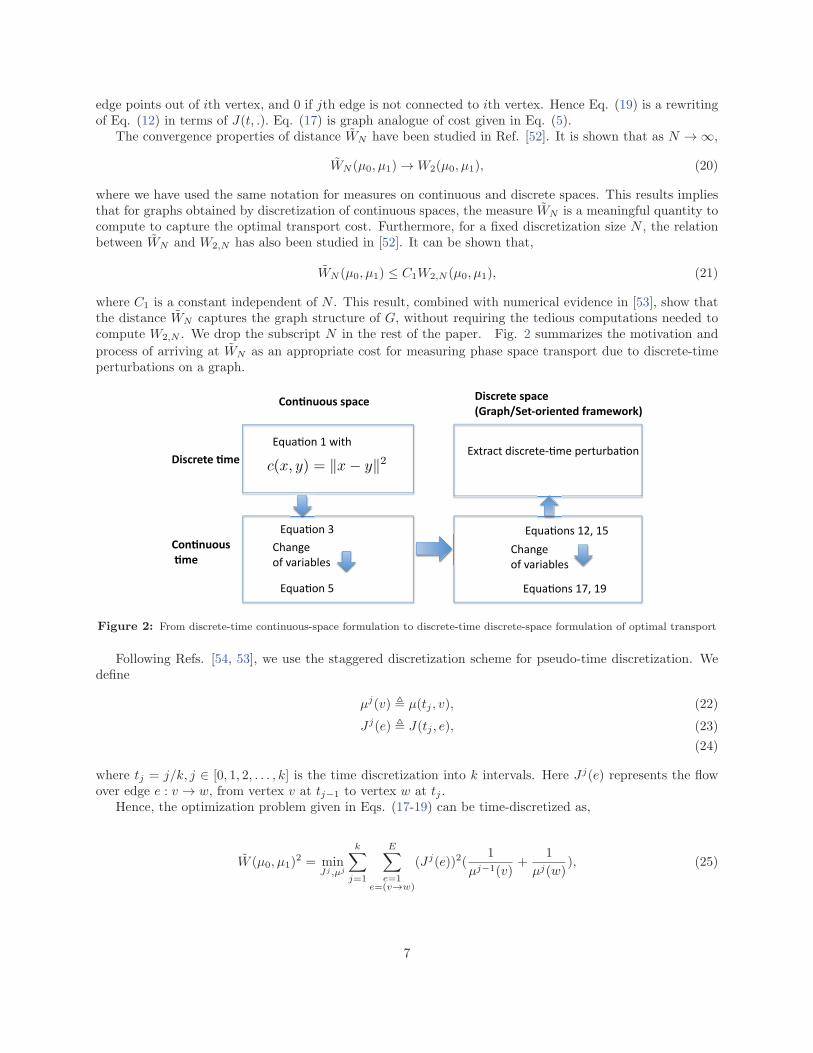
where C1 is a constant independent of N . This result, combined with numerical evidence in [53], show thatthe distance WN captures the graph structure of G, without requiring the tedious computations needed tocompute W2,N . We drop the subscript N in the rest of the paper. Fig. 2 summarizes the motivation and

process of arriving at WN as an appropriate cost for measuring phase space transport due to discrete-timeperturbations on a graph.

!"#$#%"%&'&()*+'

!"#$#%"%&'

'$,+'

-.&*/+0+'&()*+''

12/)(345+06"/.+#0+7'8/),+9"/:;'

-.&*/+0+'$,+'

!"#$%&''

()'*#+,#-.&/'!"#$%&''

()'*#+,#-.&/'

012+#32'4,/3+&2&567&'8&+29+-#6($'

0:9#6($';''

0:9#6($'<'=,2"''

c(x, y) = ‖x− y‖2

0:9#6($'>'''

0:9#6($/'<?@'<>'

0:9#6($/'<A@'<B'

Figure 2: From discrete-time continuous-space formulation to discrete-time discrete-space formulation of optimal transport

Following Refs. [54, 53], we use the staggered discretization scheme for pseudo-time discretization. Wedefine

µj(v) , µ(tj , v), (22)

Jj(e) , J(tj , e), (23)

(24)

where tj = j/k, j ∈ [0, 1, 2, . . . , k] is the time discretization into k intervals. Here Jj(e) represents the flowover edge e : v → w, from vertex v at tj−1 to vertex w at tj .

Hence, the optimization problem given in Eqs. (17-19) can be time-discretized as,

W (µ0, µ1)2 = min

Jj ,µj

k∑

j=1

E∑

e=1e=(v→w)

(Jj(e))2(1

µj−1(v)+

1

µj(w)), (25)

7

subject to the following constraints:

µj − µj−1

∆t= DTJj for j ∈ [1, 2, . . . , k], (26)

µ0 = µt0 , µn = µtf , (27)

where ∆t = 1k. We note that this form of perturbation is measure preserving by construction. The cost

function given by Eq. (25) is again of the form ‘quadratic over linear’, while the OT flow (Eq. (26)) addslinear constraints. Hence the discretized problem is convex in the problem variables (Jj , µj), and can besolved using many off-the-shelf convex solvers. Note that qj ∈ R

|V | are vertex based, and Jj ∈ R|E| are

edge based quantities. The size of the optimization problem can be quantified in terms of number of vertices|V | = N , pseudo-time discretization k, and the number of edges |E|. The graph G formed by discretizationof phase space is always sparse, since a typical vertex is at most connected to 2d neighbors, where d is thedimension of the phase space. Hence, |E| = O(N), and the problem size is O(kN). In practice, we see thatgood convergence in cost is obtained for k ∼ O(10) − O(100), and hence k ≪ N in problems of interest.Hence, this continuous (pseudo) time problem is much more tractable than solving the discrete-time problemwith the cost given by W2,N that scales as O(N2), as discussed earlier [53]. The optimization problem issolved via CVX [55] modeling platform, an open-source software for converting convex optimization problemsinto usable format for various solvers. We use the SCS [56] solver, a first-order solver for large size convexoptimization problems. This solver uses the Alternating Direction Method of Multipliers (ADMM) [57] toenable quick solution of very large convex optimization problems, with moderate accuracy.

Let us consider the optimal transport problem (without any system dynamics) for a configuration similarto the one considered in the original Brenier-Benamou paper [46]. The phase space is a unit 2-torus,and initial measure µ0 is taken to be uniform measure over a circular region in the center of the torus.The final measure µ1 is a translation of µ0, centered at the ‘corners’ of the torus. For simplicity, we useuniform measures rather than Gaussian measures considered in Ref. [46]; this does not change the solutionqualitatively. The phase space is discretized into a N = 50 × 50 grid. In Fig. 3, intermediate measures ofthe optimal transport computed via the graph based algorithm are shown. As in Ref. [46], this algorithmalso results in splitting of the initial measure into four pieces, deformation, and finally, translation of eachpiece to the nearest corner. The convergence of optimal transport cost with k is shown in Fig. 4.

3.3. Switching approach to optimal transport in nonlinear systems

Now we are ready to state our algorithm to solve the optimization problem given in Eqs. (6-9). Asmentioned in the last section, we work with measures µ supported on V . Rather than solving for T isacting on these measures, we solve for continuous pseudo-time flows which transform the measures µi to µi.Fig. 5 describes this switching approach to solving the optimization problem. In what follows, we denotepseudo-time by t, and real time by t.

Hence, the optimization problem written abstractly in Eqs. (6-9) can now be written as,

Wdyn(µt0 , µtf )2 = min

Ji(t,e)≥0,qi(t,v)≥0

n∑

i=1

∫ 1

0

∑

e=(v→w)

J i(t, e)2

2

(

1

qi(t, v)+

1

qi(t, w)

)

dt, (28)

µi = µi−1P , (29)

qi(0, v) = µi(v), qi(1, v) = µi(v) ∀v ∈ V, (30)

d

dtqi(t, .) = DTJ i(t, .) 0 ≤ t ≤ 1, (31)

µ0 = µt0 , µn = µtf . (32)

Here qi(t, .) is the pseudo-time varying measure, and J i(t, e) , qi(t, v)U i(t, e) is the flow for the ithinstance of optimal transport. To numerically solve the optimization problem, we time-discretize the advec-tion equation, i.e. Eq. (31), and corresponding flow J(., t), w.r.t pseudo-time variable t for each OT step.

8

(a) t=0 (b) t=0.1 (c) t=0.25

(d) t=0.5 (e) t=0.75 (f) t=1

Figure 3: Graph-based optimal transport of uniform measure with circular support, from the center to the corner of thetorus.

The staggered scheme for pseudo-time discretization discussed in Section 3.2 is now modified to incorporateevolution under system dynamics between the OT steps. We define

qi,j(v) , qi(tj , v), (33)

J i,j(e) , J i(tj , e), (34)

(35)

where tj = j/k, j ∈ [0, 1, 2, . . . , k] is the discretization into k intervals. Here J i,j(e) represents the flow overedge e : v → w, from vertex v at tj−1 to vertex w at tj . The resulting optimization problem can be writtenas,

Wdyn(µt0 , µtf )2 = min

Ji,j ,qi,j

n∑

i=1

k∑

j=1

E∑

e=1e=(v→w)

(J i,j(e))2(1

qi,j−1(v)+

1

qi,j(w)), (36)

subject to the following constraints:

µi = µi−1P , (37)

qi,0(v) = µi(v), qi,k(v) = µi(v) ∀v ∈ V, (38)

qi,j − qi,j−1

∆t= DTJ i,j for j ∈ [1, 2, . . . , k], (39)

µ0 = µt0 , µn = µtf , (40)

where ∆t = 1k. The cost function given by Eq. (36) is again of the form ‘quadratic over linear’, while the

evolution due to dynamics (Eq. (37)), and OT flow (Eq. (39)) are both linear constraints. The problemvariables for the convex optimization problem Eqs. (36-40) are vertex based quantities qi,j ∈ R

|V | , and edgebased quantities J i,j ∈ R

|E|. The variables in this optimization problem are O(kn(N + |E|)) = O(knN).

9

0 50 100 150395

400

405

410

415

420

k

Cost

Figure 4: Convergence of optimal transport cost Eq. (25) for the Brenier-Benamou system with time discretization k.

!"#$%!"#$%

PP

POTOT

OT OT

µ1µt0

µtfµ2

µ1

µ2

µn−1

µn

Figure 5: The switching approach to optimal transport for nonlinear systems. The transfer operator P pushes forwardmeasures µi−1 to µi over one time period. The optimal transport based perturbation step, labeled ‘OT’, and carried out inpseudo-time, pushes forward µi to µi.

4. Examples

4.1. Revisiting the Brenier-Benamou example: With linear dynamics

We first demonstrate our algorithm on a simple modification of the transport problem on torus, whichwas considered in Section 3. We consider the following discrete-time linear dynamics on the phase spaceX = T

2.

xt+1 = xt + 0.2, (41)

yt+1 = yt. (42)

This problem is solved for n = 5 time steps, and k = 20 pseudo-time discretization for representing eachperturbation with the OT step. Adding the dynamics breaks the symmetry of the system, and that of theresulting transport. In Fig. 6, the resulting transport is shown. The dynamics and final time are chosensuch that the transport in x direction can be solely accomplished by the just ‘going with flow’, i.e. withoutany perturbations. It is clear from Fig. 6 that the resulting transport indeed makes use of this fact, and theperturbations by OT only occur in the y direction.

4.2. Optimal transport in time-periodic double-gyre system

Now we consider a measure transport problem for the time-periodic double-gyre system [58]. This systemis well-studied in the dynamical systems literature, and it has been extensively used as a proving ground forseveral new computational tools related to transport and mixing [58, 48, 59, 39].

The system equations are as follows,

x = −πA sin(πf(x, t)) cos(πy), (43)

y = πA cos(πf(x, t)) sin(πy)df(x, t)

dx, (44)

10

(a) t=0 (b) t = 1, t = 0 (c) t = 1, t = 0.5

(d) t = 1, t = 1 (e) t = 2, t = 0 (f) t = 3, t = 0

(g) t = 4, t = 0 (h) t = 5, t = 0 (i) t = 5, t = 1

Figure 6: Graph-based optimal transport with dynamics: Transport of uniform measure with circular support, from thecenter to the corner of the torus with dynamics given by Eqs. (41-42).

where f(x, t) = β sin(ωt)x2 + (1− 2β sin(ωt))x is the time-periodic forcing in the system. The phase spaceis X = [0 2] × [0 1]. The dynamics of this system can be understood by a combination of geometric andstatistical tools. For the trivial case of β = 0 (i.e. no time-dependent forcing), the phase space is divided intotwo invariant sets, i.e., the left and right halves of the rectangular phase space (‘gyres’), by a heteroclinicconnection between fixed points x1 = (1, 1) and x2 = (0, 1). For non-zero β, it is instructive to study thedynamics of Poincare map F of the system, obtained by integrating the dynamics over one time period τ off . The heteroclinic connection is broken in this case, and results in a heteroclinic tangle. This heteroclinictangle leads to transport between left and right gyres via lobe-dynamics.

In this study, we use A = 0.25, β = 0.25, ω = 2π, which results in time-period τ = 1. The theory oflobe dynamics describes the qualitative and quantitative aspects of inter-gyre transport [58]. In figure 7,the unstable manifold of x1 ≈ (0.919, 1), Ux1

, and the stable manifold of x2 ≈ (1.081, 0), Sx2are shown in

green and white respectively. The lobe labeled ’A’, its pre-image F−1(A) and image F (A) are also shown.Consider the segment L = Ux1

(x1 → F (P1)) ∪ Sx2(F (P1) → x2). Then L divides phase space X into two

regions. The points that get mapped from left to right region in one iteration of F are precisely those in setA. Hence, the amount of mass transport from left to right side of L is m(A).

For further insight into transport in this system, set-oriented transfer operator methods have been utilized

11

Figure 7: Invariant manifolds and lobe-dynamics in the double-gyre system.

previously in the literature [48]. A set S is called almost-invariant if

m(F−1(S) ∩ S)

m(S)≈ 1.

Invariant and almost-invariant sets in this system can be identified by the sign structure of the secondeigenvector of the reversibilized transfer operator

R =P + P

2,

where P is the transfer operator corresponding to reverse-time dynamics. In Fig. 7, two almost-invariantsets, A1 and A2 are also shown.

We take µ0 to be the uniform measure supported on A1, and µtf to be the uniform measure supportedon A2. Both measures are normalized to sum to unity. We solve the the optimal transport problem forN = 100× 50 & k = 10 for different time horizons. We use finer grid-sizes N = 120× 60 and N = 150× 75to verify that our results are nearly independent of N . Recall that tf = nτ , where τ is the period of theflow.

In Fig. 8, the solution with n = 1, i.e., tf = τ = 1 is shown. Recall that 0 ≤ t ≤ tf is time, and 0 ≤ t ≤ 1is used to denote pseudo-time variable used in computation of the discrete-time perturbations. We use t = 0to denote beginning of each perturbation step, and t = 1 for end of the perturbation step. Since for n = 1there is only one time-step of dynamics and one discrete-time perturbation, most of the transport happensin the perturbation step. The result of sole time-step of the dynamics is shown in Fig. 8(b), which is similarto Fig. 8(a) since the initial measure is supported on AIS A1. In Figures 8(b)-(f), we show the pseudo-timeevolution of the sole discrete-time perturbation which begins at t = 1, t = 0 and ends at t = 1, t = 1.

We show the solution of the optimization problem with larger time-horizon tf = 15 in Fig. 9. In this case,a large fraction of the measure is pushed to the right via lobe-dynamics, leading to efficient transport. Therole of perturbations for large time-horizons is to push the measure into these lobes (and their pre-images).This concentration will ensure that lobe-dynamics pushes measure from left to right gyre. For instance, atthe end of third perturbation, shown in Fig. 9(b), mass has been pushed close to the sets F−1(A) and A.

12

The next application of the dynamics lead to this mass being pushed to the neighborhood of A and F (A),respectively, as shown in Fig. 9(c). This pattern is repeated over next several time-steps, eventually leadingto ‘emptying’ out of A1, and collection of mass on A2. Note that since we are solving a fixed-final timeproblem, the intermediate measures can be very different from the final target measure. The optimizationproblem allows for arbitrary mixing of intermediate measures, and optimally concentrates it on regions whichwill be transported to the right side over the next iteration. The process of concentration itself is carriedout within perturbation pseudo-time steps, as can been seen by comparing (say) Fig. 9(c) (beginning of 4thperturbation) with Fig. 9(d) (end of 4th perturbation).

In Fig. 10, we show the cost of each discrete-time perturbation over the time horizon of the problem.The use of efficient global transport given by lobe dynamics results a drastic decrease in value of the optimaltransport cost W , as shown in Fig. 11.

(a) t = 0 (b) t = 1, t = 0

(c) t = 1, t = 0.2 (d) t = 1, t = 0.5

(e) t = 1, t = 0.8 (f) t = 1, t = 1

Figure 8: Graph-based optimal transport in time-periodic double-gyre: Transport of a measure from the left AIS to the rightAIS, with tf = τ = 1. Notice since there is only one perturbation (OT) step, all of the initial measure is pushed across theinvariant manifolds to the final measure by the pseudo-time OT flow.

13

4.2.1. Localization of Perturbations

Since there exist pathways for global transport due to lobe dynamics, we expect the perturbations toincreasingly localize as time-horizon tf is increased. In other words, we expect that for large time horizons,globally optimal perturbations would not involve transport which can accomplished for ‘free’. To quantifythis behavior, we compute the map T i : R|V | → R

|V | corresponding to ith perturbation in the optimizationproblem given by Eqs. (36-40). We first reconstruct the advection map over each pseudo-time step in ithperturbation, T i,j : R|V | → R

|V |, using an infinitesimal-generator approximation [60], as follows.

T i,j(v, w) =

∑

e:w→v

U i,j(e) v 6= w

1−∑

e:v→v

U i,j(e) otherwise(45)

Then, T i is obtained as the composition map of k pseudo-time advection maps, i.e T i = T i,kT i,k−1 . . . T i,1.We define a distance Dl on the set of all T i, i = 1, 2, n as follows.

Dl =1

δxmax

i∈[1,2,...,n]maxv∈V

max{w|T i(v,w)>0}

d∞(v, w), (46)

where d∞(v, w) is the greater of the distances in x and y directions between centers of boxes v and w. HenceDl is simply the greatest distance in x or y directions that any mass is moved by any of the n perturbations,divided by δx. Here δx is the length of Bi. In Fig. 12, we plot the measure Dl for various values of tf .It is clear from this plot that along with decreasing transport cost, the perturbations tend to localize withincreasing tf . However, there seems to be a minimum value of Dl ≈ 8, even for large tf , indicating a lowerlimit on the ‘radius’ of perturbation for reaching the desired final measure.

4.3. Optimal mixing enhancement in time-periodic Double-Gyre system

Next, we apply our algorithm to the problem of optimal enhancement of finite-time mixing. We aim toobtain optimal perturbations at discrete times that lead to complete mixing in given finite time. We chooseµt0 to be the uniform measure supported on A1, and µtf to be the uniform measure over phase space X.Both measures are normalized to unity as before.

Note again that this problem setting is different than those considered in previous works on mixingmeasures and optimal mixing [21, 20, 39], since the aim is to minimize a cost associated with phase spacetransport due to applied perturbations, rather than maximizing ‘mixedness’ at final time. Furthermore, sincewe are using a set-oriented framework, there is an inherent minimal scale present in the problem, i.e. the sizeof each box Bi or vertex v. Inhomogeneity in the measure at length scales below this size are ignored, andhence, complete mixing in this context implies that inhomogeneities for all scales above the size of smallestbox in the partition have been removed. We also note that using set-oriented approach for propagatingmeasures is known to cause artificial diffusion.

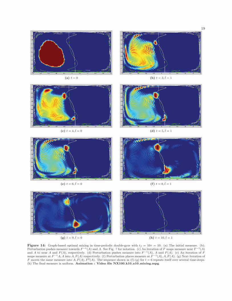
The solution sequence for n = 1 is shown in Fig. 13. In this short time-horizon mixing problem, only someof the mass is transported directly across the invariant manifolds to the right side, in contrast with the caseof n = 1 transport problem considered earlier. The rest of the mass is mixed on the left side by a smearingtype action, and the mass transported to right is similarly mixed. For the long time-horizon case shown inFig. 14, the situation is analogous. Some of the perturbation effort is spent in smearing the measure on eachside, while rest of time is used to push it into the lobes (and their pre-images) to enable global transport of‘half’ of the measure to the the right side. Both these actions are carried out simulataneously. For instance,the third perturbation places some mass near F−1(A) and A, while mixing other mass all across the leftside, shown in Fig. 14(c). The action of P moves mass to A and F (A) respectively, as shown in Fig. 14(d).This process is again repeated over the rest of the time-horizon. Fig. 14(g) shows the final lobe transportfrom left to right side, while the rest of the measure is almost fully mixed. In Fig. 15, we show the cost ofeach discrete-time perturbation over the time horizon of the problem. The use of efficient global transportgiven by lobe dynamics again results a large decrease in value of the optimal mixing cost W , as shown inFig. 16.

14

In Fig. 17, we plot the measure Dl for various values of tf . It can be seen that along with decreasingmixing cost, the perturbations tend to localize with increasing tf . Compared to the transport case, theoptimal mixing solution shows higher localization with increasing tf . Hence, the localized perturbationsplay a dual role. On one hand, they enable the use of lobe dynamics for global transport by concentratingmeasure in pre-images of lobes (the measure concentration can be interpreted as a de-mixing process). Onthe other hand, they increase local mixing which leads to homogenization at a faster rate than that achievedby natural dynamics alone. The localization information obtained from computing Dl can be valuable indesigning efficient short-time mixing protocols, and formulating an optimization problem with localizationconstraints on the perturbations.

5. Conclusions and Extensions

We have presented a framework for computing provably globally optimal perturbations for transporting agiven initial phase space measure to an arbitrary final measure in finite time for nonlinear dynamical systems.We model the discrete-time perturbations as maps which result from Monge-Kantorovich optimal transporton graphs. Our work represents a first step towards combining the set-oriented transfer operator methodswith optimal transport theory, via use of graph-based optimal transport concepts. Our results show thatthe resulting transport exploits efficient global transport available via mechanisms such as lobe-dynamics,as the time-horizon of the problem is increased.

Several extensions of this work are desirable. The extension to dynamical systems with arbitrary timedependence is straightforward. The interesting case to study in these systems is optimal transport betweencoherent sets. By exploiting efficient phase space discretization techniques, such as those employed in GAIO[9], one can hope to improve the efficiency of the resulting optimal transport algorithms, and apply theframework to higher dimensional dynamical systems. Graph pruning algorithms can be employed to removeedges which are not likely to be used during the perturbation step [61].

While we give numerical evidence that the perturbation cost decreases with increasing time-horizon, andthat the perturbation becomes increasingly localised, it is desirable to obtain more quantitative estimates ofsuch behavior, possibly via a rigorous convergence analysis of the problem in the long-time limit. We havenot explictly considered control constraints in the current work. By using edge weights on edges E whichreflect some control cost, this framework can potentially be extended to obtain perturbations which canbe implemented via available control mechanisms, and result in optimal control cost. This is a challengingproblem since it involves deriving conditions on controllability or reachability of measures in discrete-timesetting. One way to make progress would be relax the final condition to only approximately achieve thefinal distribution. For chaotic systems, this relaxed version should result in a well-posed problem under mildassumptions. Connections with work in the closely related area of occupation measures [31] and Lyapunovmeasures [28] also need to be explored. Comparing optimal mixing analysis given in this paper with priorwork which has exploited a different optimal transport measure to obtain bounds on finite time mixing [22]is another topic of possible interest.

Recent methods in obtaining Lagrangian coherent structures and coherent sets in finite-time non-autonomoussystems have used variational formulations of transport under nonlinear dynamics [14, 62]. It would be fruit-ful to develop connections of these objects with optimal mass transportation theory, since there already existsuch connections in the autonomous Hamiltonian dynamics case [43].

Finally, it is of great interest to obtain a set-oriented approach to continuous-time optimal transport for-mulation of nonlinear systems with control vector fields, i.e. obtaining control laws that implement possiblynon-holonomic optimal transport of measures in nonlinear dynamical systems. This topic is considered in aforthcoming work.

6. Acknowledgments

We thank the anonymous reviewers for their careful reading of the manuscript, and helpful suggestionsthat have led to significant improvement in the quality of this work.

15

(a) t = 0 (b) t = 3, t = 1

(c) t = 4, t = 0 (d) t = 4, t = 1

(e) t = 5, t = 0 (f) t = 6, t = 1

(g) t = 7, t = 0 (h) t = 15, t = 1

Figure 9: Graph-based optimal transport in time-periodic double-gyre: Transport of a measure from the left AIS to the rightAIS, with tf = 15τ = 15. (a) The initial measure. (b). Perturbation pushes measure towards F−1(A) and A. See Fig. 7for notation. (c) An iteration of F maps measure from neighborhood of A to neighborhood of F (A). (d) Perturbation pushesmeasure into F−1(A), A and F (A). (e) An iteration of F maps measure at F−1A,A into A,F (A) respectively. (f) Perturbationplaces measure at F−1(A), A, F (A). (g) Next iteration of F moves the same measure into A,F (A), F 2(A). The sequence shownin (f)-(g) for t = 6 repeats itself over several time-steps. (h) The final measure is supported on A2. Animation:Video fileNX100 k10 n15 transport.mpg

17

0 5 10 154

4.5

5

5.5

6

t

Cost

of

transport

(P

ert

urb

ation)

Figure 10: The cost of discrete-time perturbations T i, i = 1 to 15, for the case shown in Fig. 9.

0 5 10 150

500

1000

1500

2000

2500

3000

3500

tf

Cost

of

transport

(P

ert

urb

ation)

Figure 11: The optimal transport cost (given by Eq. 36) for the double-gyre system for transport between the two measureswith supports A1 and A2 respectively, for various time-horizons tf . For small time-horizons, perturbations push bulk of themeasure directly into the right side. As the time-horizon increases, a larger fraction of the mass is pushed to the right vialobe-dynamics, leading to efficient transport. The role of perturbations for large time horizons is to push the measure into theselobes (and their pre-images).

5 10 15 20 25 305

10

15

20

Dl

tf

Figure 12: The measure Dl, defined in Eq. (46), as a function of time-horizon tf . Decay in the the value of Dl implies thatperturbations get increasingly localized as time-horizon is increased

18

(a) t = 0 (b) t = 1, t = 0

(c) t = 1, t = 0.2 (d) t = 1, t = 0.5

(e) t = 1, t = 0.8 (f) t = 1, t = 1

Figure 13: Graph-based optimal mixing in time-periodic double-gyre with tf = τ = 1. Notice since there is only oneperturbation (OT) step, all of the initial measure is pushed across the invariant manifolds to the final measure by the pseudo-time OT flow).

19

(a) t = 0 (b) t = 3, t = 1

(c) t = 4, t = 0 (d) t = 5, t = 1

(e) t = 6, t = 0 (f) t = 8, t = 1

(g) t = 9, t = 0 (h) t = 10, t = 1

Figure 14: Graph-based optimal mixing in time-periodic double-gyre with tf = 10τ = 10. (a) The initial measure. (b).Perturbation pushes measure towards F−1(A) and A. See Fig. 7 for notation. (c) An iteration of F maps measure near F−1(A)and A to near A and F (A), respectively. (d) Perturbation pushes measure into F−1(A), A and F (A). (e) An iteration of Fmaps measure at F−1A,A into A,F (A) respectively. (f) Perturbation places measure at F−1(A), A, F (A). (g) Next iteration ofF moves the same measure into A,F (A), F 2(A). The sequence shown in (f)-(g) for t = 6 repeats itself over several time-steps.(h) The final measure is uniform. Animation : Video file NX100 k10 n10 mixing.mpg

20

1 2 3 4 5 6 7 8 9 102.8

3

3.2

3.4

3.6

3.8

4

4.2

t

Cost

of

Mix

ing (

Pert

urb

ation)

Figure 15: The cost of discrete-time perturbations T i, i = 1 to 10, for the case shown in Fig. 14.

0 5 10 150

200

400

600

800

1000

1200

1400

tf

Cost

of

Mix

ing (

Pert

urb

ation)

Figure 16: The optimal mixing cost (given by Eq. 36) for the double-gyre system for mixing the measure supported on A1,for various time-horizons tf . For small time-horizons, perturbations push half of the measure directly into the right side, beforesmearing it to make final measure uniform. As the time-horizon increases, a larger fraction of the mass is pushed to the rightvia lobe-dynamics, leading to drastically lower mixing cost. The role of perturbations for large time horizons is to push themeasure into these lobes (and their pre-images), and later smear it uniformly in the domain.

5 10 15 20 25 30

5

10

15

20

Dl

tf

Figure 17: The measure Dl, defined in Eq. (46), as a function of time-horizon tf . Decay in the the value of Dl implies thatperturbations get increasingly localized as time-horizon is increased.

References

[1] J. M. Ottino, S. Wiggins, Introduction: mixing in microfluidics, Philosophical Transactions: Mathe-matical, Physical and Engineering Sciences (2004) 923–935.

[2] S. Wiggins, J. M. Ottino, Foundations of chaotic mixing, Philosophical Transactions of the Royal Societyof London A: Mathematical, Physical and Engineering Sciences 362 (1818) (2004) 937–970.

[3] W. Koon, M. Lo, J. Marsden, S. Ross, Dynamical Systems, the Three-Body Problem and Space MissionDesign, Marsden Books, 2008.

[4] J. D. Meiss, Symplectic maps, variational principles, and transport, Rev. Mod. Phys. 64 (1992) 795–848.

[5] J. Marsden, S. Ross, New methods in celestial mechanics and mission design, Bulletin of the AmericanMathematical Society 43 (1) (2006) 43–73.

[6] P. Boyland, H. Aref, M. Stremler, Topological fluid mechanics of stirring, Journal of Fluid Mechanics362 (2000) 1019–1036.

[7] J.-L. Thiffeault, M. D. Finn, Topology, braids and mixing in fluids, Philosophical Transactions of theRoyal Society of London A: Mathematical, Physical and Engineering Sciences 364 (1849) (2006) 3251–3266.

[8] M. Dellnitz, O. Junge, On the approximation of complicated dynamical behavior, SIAM Journal onNumerical Analysis 36 (1998) 491–515.

[9] M. Dellnitz, G. Froyland, O. Junge, The algorithms behind GAIO – set oriented numerical methodsfor dynamical systems, in: B. Fiedler (Ed.), Ergodic Theory, Analysis, and Efficient Simulation ofDynamical Systems, Springer, Berlin-Heidelberg-New York, 2001, pp. 145–174.

[10] A. Lasota, M. Mackey, Chaos, Fractals and Noise, Springer-Verlag, New York, 1994.

[11] E. M. Bollt, N. Santitissadeekorn, Applied and Computational Measurable Dynamics, Vol. 18, SIAM,2013.

[12] S. Wiggins, Chaotic transport in dynamical systems, Vol. 2, Springer Science & Business Media, 2013.

[13] G. Haller, Finding finite-time invariant manifolds in two-dimensional velocity fields, Chaos 10 (2000)99–108.

[14] G. Haller, Lagrangian coherent structures, Annual Review of Fluid Mechanics 47 (2015) 137–162.

[15] C. Senatore, S. D. Ross, Fuel-efficient navigation in complex flows, in: 2008 American Control Confer-ence, IEEE, 2008, pp. 1244–1248.

[16] P. Grover, C. Andersson, Optimized three-body gravity assists and manifold transfers in end-to-endlunar mission design, in: 22nd AAS/AIAA Space Flight Mechanics Meeting, Vol. 143, American Astro-nautical Society, 2012, pp. 1189–1203.

[17] S. Balasuriya, Optimal perturbation for enhanced chaotic transport, Physica D: Nonlinear Phenomena202 (3) (2005) 155–176.

[18] S. Balasuriya, Dynamical systems techniques for enhancing microfluidic mixing, Journal of Microme-chanics and Microengineering 25 (9) (2015) 094005.

[19] G. Mathew, I. Mezic, L. Petzold, A multiscale measure for mixing, Physica D: Nonlinear Phenomena211 (1) (2005) 23–46.

21

[20] G. Mathew, I. Mezic, S. Grivopoulos, U. Vaidya, L. Petzold, Optimal control of mixing in stokes fluidflows, Journal of Fluid Mechanics 580 (2007) 261–281.

[21] Z. Lin, J.-L. Thiffeault, C. R. Doering, Optimal stirring strategies for passive scalar mixing, Journal ofFluid Mechanics 675 (2011) 465–476.

[22] C. Seis, Maximal mixing by incompressible fluid flows, Nonlinearity 26 (12) (2013) 3279.

[23] G. Iyer, A. Kiselev, X. Xu, Lower bounds on the mix norm of passive scalars advected by incompressibleenstrophy-constrained flows, Nonlinearity 27 (5) (2014) 973.

[24] P. Hassanzadeh, G. P. Chini, C. R. Doering, Wall to wall optimal transport, Journal of Fluid Mechanics751 (2014) 627–662.

[25] G. Froyland, K. Padberg, M. England, A. Treguier, Detecting coherent oceanic structures via transferoperators, Physical Review Letters 98:224503.

[26] O. Junge, H. M. Osinga, A set oriented approach to global optimal control, ESAIM: Control, optimisa-tion and calculus of variations 10 (2) (2004) 259–270.

[27] S. D. Ross, S. Jerg, O. Junge, Optimal capture trajectories using multiple gravity assists, Communica-tions in Nonlinear Science and Numerical Simulations 14 (12) (2009) 4168–4175.

[28] U. Vaidya, P. G. Mehta, Lyapunov measure for almost everywhere stability, IEEE Transactions onAutomatic Control 53 (1) (2008) 307–323.

[29] U. Vaidya, P. G. Mehta, U. V. Shanbhag, Nonlinear stabilization via control lyapunov measure, IEEETransactions on Automatic Control 55 (6) (2010) 1314–1328.

[30] A. Raghunathan, U. Vaidya, Optimal stabilization using lyapunov measures, IEEE Transactions onAutomatic Control 59 (5) (2014) 1316–1321.

[31] J. B. Lasserre, D. Henrion, C. Prieur, E. Trelat, Nonlinear optimal control via occupation measures andlmi-relaxations, SIAM Journal on Control and Optimization 47 (4) (2008) 1643–1666.

[32] C. Villani, Topics in optimal transportation, no. 58, American Mathematical Society, 2003.

[33] A. Ghosh, P. Fischer, Controlled propulsion of artificial magnetic nanostructured propellers, Nano letters9 (6) (2009) 2243–2245.

[34] U. K. Cheang, K. Lee, A. A. Julius, M. J. Kim, Multiple-robot drug delivery strategy through coordi-nated teams of microswimmers, Applied physics letters 105 (8) (2014) 083705.

[35] K. E. Peyer, L. Zhang, B. J. Nelson, Bio-inspired magnetic swimming microrobots for biomedical ap-plications, Nanoscale 5 (4) (2013) 1259–1272.

[36] K. Elamvazhuthi, S. Berman, Optimal control of stochastic coverage strategies for robotic swarms, in:2015 IEEE International Conference on Robotics and Automation (ICRA), IEEE, 2015, pp. 1822–1829.

[37] R. Wood, R. Nagpal, G.-Y. Wei, Flight of the robobees, Scientific American 308 (3) (2013) 60–65.

[38] P. Lermusiaux, T. Lolla, P. Haley Jr, K. Yigit, M. Ueckermann, T. Sondergaard, W. Leslie, Science ofautonomy: Time-optimal path planning and adaptive sampling for swarms of ocean vehicles, SpringerHandbook of Ocean Engineering: Autonomous Ocean Vehicles, Subsystems and Control.

[39] G. Froyland, C. Gonzalez-Tokman, T. M. Watson, Optimal mixing enhancement by local perturbation,SIAM Review 58(3) (2016) 494–513.

[40] G. Froyland, N. Santitissadeekorn, Optimal mixing enhancement, arXiv preprint arXiv:1610.01651.

22

[41] Y. Chen, T. T. Georgiou, M. Pavon, Optimal steering of a linear stochastic system to a final probabilitydistribution, part 1, IEEE Transactions on Automatic Control 61 (5) (2016) 1158–1169.

[42] A. Figalli, L. Rifford, Mass transportation on sub-riemannian manifolds, Geometric And FunctionalAnalysis 20 (1) (2010) 124–159.

[43] P. Bernard, B. Buffoni, Optimal mass transportation and mather theory, arXiv preprint math/0412299.

[44] L. Ambrosio, N. Gigli, G. Savare, Gradient flows: in metric spaces and in the space of probabilitymeasures, Springer Science & Business Media, 2008.

[45] F. Santambrogio, Optimal transport for applied mathematicians, Progress in Nonlinear DifferentialEquations and their applications 87.

[46] J.-D. Benamou, Y. Brenier, A computational fluid mechanics solution to the monge-kantorovich masstransfer problem, Numerische Mathematik 84 (3) (2000) 375–393.

[47] S. Boyd, L. Vandenberghe, Convex optimization, Cambridge university press, 2004.

[48] G. Froyland, K. Padberg, Almost-invariant sets and invariant manifolds – connecting probabilistic andgeometric descriptions of coherent structures in flows, Physica D 238(16) (2009) 1507–1523.

[49] S. M. Ulam, Problems in modern mathematics, Courier Corporation, 2004.

[50] S. Berman, A. Halasz, M. A. Hsieh, V. Kumar, Optimized stochastic policies for task allocation inswarms of robots, IEEE Transactions on Robotics 25 (4) (2009) 927–937.

[51] A. Chapman, M. Mesbahi, Advection on graphs, in: 2011 50th IEEE Conference on Decision andControl and European Control Conference, IEEE, 2011, pp. 1461–1466.

[52] N. Gigli, J. Maas, Gromov–hausdorff convergence of discrete transportation metrics, SIAM Journal onMathematical Analysis 45 (2) (2013) 879–899.

[53] J. Solomon, R. Rustamov, L. Guibas, A. Butscher, Continuous-flow graph transportation distances,arXiv preprint arXiv:1603.06927.

[54] N. Papadakis, G. Peyre, E. Oudet, Optimal transport with proximal splitting, SIAM Journal on ImagingSciences 7 (1) (2014) 212–238.

[55] M. Grant, S. Boyd, Y. Ye, CVX: Matlab software for disciplined convex programming (2008).

[56] B. O’Donoghue, E. Chu, N. Parikh, S. Boyd, Operator splitting for conic optimization via homogeneousself-dual embedding, arXiv preprint arXiv:1312.3039.

[57] J. Eckstein, W. Yao, Augmented lagrangian and alternating direction methods for convex optimization:A tutorial and some illustrative computational results, RUTCOR Research Reports 32.

[58] F. Lekien, C. Coulliette, Chaotic stirring in quasi-turbulent flows, Philosophical Transactions of theRoyal Society of London A: Mathematical, Physical and Engineering Sciences 365 (1861) (2007) 3061–3084.

[59] P. Tallapragada, S. D. Ross, A set oriented definition of finite-time lyapunov exponents and coherentsets, Communications in Nonlinear Science and Numerical Simulation 18 (5) (2013) 1106–1126.

[60] G. Froyland, O. Junge, P. Koltai, Estimating long-term behavior of flows without trajectory integration:The infinitesimal generator approach, SIAM Journal on Numerical Analysis 51 (1) (2013) 223–247.

[61] D. D. Harabor, A. Grastien, et al., Online graph pruning for pathfinding on grid maps., in: AAAI, 2011.

[62] G. Froyland, Dynamic isoperimetry and the geometry of lagrangian coherent structures, Nonlinearity28 (10) (2015) 3587.

23