some characteristic properties of a decorated ferrimagnetic ising system

Physica A 303 (2002) 507–524www.elsevier.com/locate/physa

Some characteristic properties of adecorated ferrimagnetic Ising system

T. Kaneyoshi∗Department of Natural Science Informatics, School of Informatics and Sciences, Nagoya University,

Chikusa-ku, Nagoya, 464-8601, Japan

Received 10 July 2001

Abstract

The magnetic properties (phase diagram, magnetization curve, spin correlation functions,internal energy and magnetic speci+c heat) of a decorated ferrimagnetic square lattice composedof three magnetic atoms are investigated on the basis of the di.erential technique. The systemcan show many interesting properties which have not been obtained in the previous decoratedIsing models. In particular, the possibility of two compensation points can be found more easilythan that of the previous systems discussed in J. Phys. Soc. Jpn. 70 (2001) 884 and the speci+cheat of the present system exhibits various characteristic features in the ordered phase belowits transition temperature, depending on the spin of decorated atom and the value of uniaxialanisotropy parameter. c© 2002 Elsevier Science B.V. All rights reserved.

Keywords: Ising model; Speci+c heat; Ferrimagnetism; Compensation point

1. Introduction

Ferrimagnetism has been extensively investigated in the past both experimentally andtheoretically. One characteristic property in a ferromagnetic material is the shape of thetemperature dependence of spontaneous magnetization. Among these works, Syozi andNakano introduced a decorated two sublattice ferrimagnetic Ising model many years ago[1]. The system consists of two magnetic atoms A and B with SA =± 1 and SB =± S(S¿ 1), where the B sites decorate the bonds between A sites. The model system

∗ Fax: +81-52-789-4846.E-mail address: [email protected] (T. Kaneyoshi).

0378-4371/02/$ - see front matter c© 2002 Elsevier Science B.V. All rights reserved.PII: S 0378 -4371(01)00491 -5

508 T. Kaneyoshi / Physica A 303 (2002) 507–524

can be solved exactly for low-dimensional systems, but the temperature dependence ofspontaneous magnetization in the system takes the form already predicted by NEeel [2].On the other hand, Kaneyoshi has introduced a decorated ferrimagnetic Ising systemcomposed of SA = 1

2 atoms and SB = S (S ¿ 12 ) atoms with a uniaxial anisotropy [3,4].

In contrast to the prediction in Ref. [1], he has shown that the possibility of twocompensation points can be found exactly for the thermal variation of spontaneousmagnetization in the system with a negative anisotropy, when the value of S is selectedas an integer. The system has exhibited a number of characteristic phenomena, whichare not predicted in the NEeel theory [3–5].Very recently, a decorated ferrimagnetic Ising square lattice consisting of three mag-

netic atoms A, B and C with spins SA = 12 , SB =

12 and SC ¿ 1

2 has been studied byKaneyoshi [6] on the basis of the di.erential operator technique [7,8]. The transitiontemperature and magnetization curve have been discussed by using the analytic expres-sions of the Bethe–Peierls approximation [9]. The system can exhibit some character-istic phenomena not predicted by the NEeel theory, such as two compensation points inthe system with a negative uniaxial anisotropy on C atoms when the spin con+gurationof decorated atoms B and C is directed oppositely. The possibility of two compensationpoints had also been pointed in the work of Hattori [10], although his model systemwas arti+cial.The aim of this work is again to study the magnetic properties (phase diagram,

magnetization curve, spin correlation functions, internal energy and magnetic speci+cheat) of the decorated ferrimagnetic Ising square lattice composed of three magneticatoms A, B and C with SA = 1

2 , SB =1 and SC = S (S ¿ 1) within the frameworkof the di.erential operator technique [7,8]. The e.ects of two uniaxial anisotropies(DB and DC) on B and C atoms to the magnetic properties are discussed in de-tail. In Section 2, the general formulation is given, which is valid for both the fer-romagnetic and the ferrimagnetic system. The transition temperature, magnetizationcurve, spin correlation functions, internal energy and the magnetic speci+c heat ofthe system are discussed by using the analytic expressions of the Bethe–Peierls ap-proximation [9], although the expression for determining the compensation temper-ature in a ferrimagnetic system can be obtained exactly. In Section 3, the numer-ical results of the ferrimagnetic system are presented for two values of S (S = 3

2and 2). We +nd that the magnetic properties of the system may exhibit a varietyof interesting behaviors depending on the value of S and the ratio (DB=DC) of theanisotropies.

2. Formulation

We consider the decorated Ising ferromagnetic or ferrimagnetic square lattice com-posed of three magnetic atoms A, B and C where all sites at square lattice are occupiedby a magnetic A atom with SA = 1

2 and the decorated sites are occupied by a magneticB atom with SB =1 and a magnetic C atom with SC = S (S ¿ 1) in a de+nite way, as

T. Kaneyoshi / Physica A 303 (2002) 507–524 509

Fig. 1. The spatial con+guration of the decorated Ising square lattice composed of three magnetic atoms,like the Verwey order. The white circles denote A atoms with spin SA = 1

2 , the shaded circles represent Batoms with spin SB = 1 and the black circles are C atoms with spin SC = S (¿ 1).

shown in Fig. 1. The Hamiltonian of the system is given by

H=−∑(im)

Jim�zi S

zm −

∑(in)

Jin�zi S

zn − J ′′∑

(ij)

�zi �

zj

−DB

∑m

(Szm)

2 − DC

∑n

(Szn)

2 ; (1)

where the +rst three summations run over the nearest-neighbor pairs. �zi is the spin- 12

operator for the A atoms. Szm and Sz

n are, respectively, the spin-1 operator for the Batoms and the spin-S operator for the C atoms. DB and DC are the uniaxial anisotropyconstants on B and C atoms. We assume that the exchange interactions Jim and Jin cantake the two values, namely Jim =± J and Jin =± J ′.The total magnetization of the system is given by

(M=N )=FA + mB + mC (2)

with

FA = 〈�zi 〉; mB = 〈Sz

m〉; mC = 〈Szn〉 ; (3)

where N is the total number of A atoms.


By the use of the di.erential operator technique [7,8], as has been discussed inRefs. [3,4,6], the total magnetization (2) can be rewritten exactly in the form

(M=N )=FA[1± 2FB(J )± 2FC(J ′)] ; (4)

where the ± sign represents the ferromagnetic (parallel) or ferrimagnetic (antiparallel)spin con+guration of B and C atoms, in comparison with the spin direction of A atoms.The function FB(x) is de+ned by

FB(x)=2 sinh(�x)

2 cosh(�x) + exp(−�DB); (5)

where �=1=kBT . The function FC(x) depends on the value of S, whose expressioncan be easily derived (see Refs. [3,4,6]).Let us now take the − sign in (4). Then, the system shows a ferrimagnetic spin

con+guration, where the spin directions of B and C atoms are directed to the oppositedirection of the A atomic spin. Accordingly, there may be a compensation temper-ature Tk at which the total magnetization reduces to zero even though FA �=0. Thecompensation point in the ferrimagnetic system seems to be exactly given by

1=2[FB(J ) + FC(J ′)] : (6)

In order to get the internal energy de+ned by U = 〈H〉, we need to know the spin–spin correlation functions 〈�z

i Szm〉 and 〈�z

i Szn〉 as well as the expectation values 〈(Sz

m)2〉

and 〈(Szn)

2〉. Using the Ising spin identities and the di.erential operator technique [7,8],the expectation value 〈(Sz

p)2〉 (p=m or n) can be expressed exactly in the form [11]

〈(Szp)

2〉= 〈[cosh(h�=2)± 2�zi+� sinh(h�=2)]

×[cosh(h�=2)± 2�zi sinh(h�=2)]〉Gq(x)|x=0

= 12 [Gq(h) + Gq(0)] + 2〈�z

i+��zi 〉[Gq(h)− Gq(0)] ; (7)

where h= J for q=B or h= J ′ for q=C, �= @=@x is a di.erential operator and thefunction Gq(x) for q=B is de+ned by

GB(x)=2 cosh(�x)

2 cosh(�x) + exp(−�DB): (8)

The function Gq(x) for q=C depends on the value of S, and its explicit form can beeasily obtained (see Refs. [3,4,6]).By the use of the same procedure as that of 〈(Sz

p)2〉 (p=m or n), the correlation

function 〈�zi S

zp〉 (p=m or n) can be expressed exactly as

±〈�zi S

zp〉= [14 + 〈�z

i+��zi 〉]Fq(h) (q=B or C) ; (9)


where h= J for q=B or h= J ′ for q=C. Substituting (9) and (7) into the expressionof U , it can be rewritten exactly in the form

UN =− 1

4 [JFB(J ) + 2DB{GB(J ) + GB(0)}]

− 14 [J

′FC(J ′) + 2DC{GC(J ′) + GC(0)}]

−G1[JFB(J ) + J ′′ + 2DB{GB(J )− GB(0)}]

−G2[J ′FC(J ′) + J ′′ + 2DC{GC(J ′)− GC(0)}] (10)

with

G1 = 〈�zi �

zi+�〉; G2 = 〈�z

i �zi+�′〉 ; (11)

where 〈�zi+��

zi 〉 and 〈�z

i+�′�zi 〉 represent, respectively, the spin–spin correlation functions

of the parallel and perpendicular directions in Fig. 1.The speci+c heat C of the system can be determined from

C=N = @=@T (U=N ) : (12)

Thus, one should notice that C and U are independent of the ± sign of the exchangeinteractions in (1).The problem now is how to evaluate the sublattice magnetization FA and the spin–

spin correlation functions G1 and G2, in order to study the magnetic properties of thesystem. As discussed in Refs. [3,4,6,11], one can use the decoration–iteration trans-formation [12], in order to get the e.ective Hamiltonian He. for the square latticedescribed by

He. =−∑(i; �)

JR� �

zi �

zi+� ; (13)

where JR� can take two values depending on the direction. They are given by

JR� = J ′′ + JH

e. for the horizontal direction in Fig: 1

and

JR� = J ′′ + J P

e. for the perpendicular direction in Fig: 1: (14)

The two e.ective interactions JHe. and J P

e. can be obtained easily by the use of therelation∑

Szp

exp[�Jip(�zi + �z

i+�)Szp + �Dq(Sz

p)2]=A exp[�J

e.�zi �

zi+�] ; (15)

where =H or P and Dq =DB or DC, depending on whether p is selected as p=mor p= n. The JH

e. is a function of DB and the J Pe. depends on the values of S and DC

(see Refs. [3,4,6,10]).Using the e.ective Hamiltonian (13), the analytic solutions for the anisotropic Ising

square lattice can be used for the evaluation of FA, G1 and G2 in the present system,


as noted in Ref. [6]. They have been solved within the framework of the Bethe–Peierlsapproximation [9]. By the use of the expressions, the sublattice magnetization FA isgiven by

FA =12

[1− 4

2 + !

]1=2(16)

with

!=2cosh[t(1− o)]− 2[exp(t) + exp(ot)] + exp[t(1 + o)] ;

where t= �JHe. and o= J P

e. =JHe. . At the critical temperature T =TC, the magnetization

(16) reduces to zero. The TC can be determined from

1= exp(−JHe.�C=2) + exp(−J P

e.�C=2) (17)

with

�C =1=kBTC :

Furthermore, for T6TC, the expressions of G1 and G2 are given by

G1 = (FA)2 + $1[( 14 )− (FA)2] ;

G2 = (FA)2 + $2[( 14 )− (FA)2] (18)

with

$1 = exp[�JHe. (1− o)]=[exp(�JH

e. )− 1] ;

$2 = exp[�J Pe. (o− 1)]=[exp(�J P

e. )− 1] (19)

and for T¿TC

G1 =14tanh

(�JH

e.

4

);

G2 =14tanh

(�J P

e.

4

): (20)

3. Numerical results

In this section, we investigate the magnetic properties (phase diagram, magnetizationcurve, spin–spin correlation functions, internal energy and magnetic speci+c heat) ofthe decorated ferrimagnetic square lattice by solving (6), (17), (16), (18)–(20), (10)and (12) numerically. Let us at +rst introduce the parameters de+ned by

a= J ′=J; b= J ′′=J; d=DB=J and r=DC=DB : (21)

In the following numerical calculations, we assume that a=1 for simplicity, althoughthe magnetic properties may depend delicately on the parameter a, as discussed in


Ref. [6]. Let us now study the e.ects of r and S on the magnetic properties ofthe present system. Then, the two values of S (S = 3

2 and 2) are selected forclari+cation.

3.1. Phase diagram

Fig. 2 shows the phase diagrams (TC and Tk versus d) of the two systems with S = 32

and 2. The Tk curves have been obtained by solving (6) and they represent the com-pensation temperature in each ferrimagnetic system, where the spin con+gurations of Band C atoms are directed opposite to the spin direction of A atoms. Each Tk curve (ex-cept the one labeled r=5:0 in Fig. 2(a)) shows the reentrant phenomenon (the doublevalues) in the restricted region of negative d. It indicates that one can +nd the possi-bility of two compensation points, when the appropriate values of d and r are selectedin the system. In particular, one should notice that the possibility of two compensationpoints can be found even when both the spin con+gurations of the B and C atoms areselected opposite to the spin direction of the A atoms. The fact is clearly di.erent fromthe previous results in Ref. [6]. Furthermore, as has been reviewed in the introductionof Ref. [6], it will be interesting to study the possibility of two compensation points ina ferrimagnetic system experimentally and theoretically. The occurrence of two com-pensation points may be of great technological importance, since between these pointsonly a small driving +eld is required to change the sign of the resultant magnetization.In fact, this property may open a new and useful possibility for the thermomagneticrecording, as has been discussed in Ref. [13] for the ferrimagnetic multiplayer +lmswith two compensation points. The Tk curve labeled r=5:0 in Fig. 2(a) is presentedin the +gure, since it does not also exhibit the monotonic variation as a functionof d.

3.2. Magnetization curves

Looking at the results of phase diagram (or Fig. 2), let us at +rst check whether theferrimagnetic systems with S = 3

2 and 2 may exhibit two compensation points in thetemperature region below TC, taking only the − sign in (4) and selecting the appropriateparameters in Fig. 2. Fig. 3 shows the temperature dependences of total magnetiza-tion (or the absolute value |M |=N ) in the systems, namely Figs. 3(a) and (b) corre-spond, respectively, to Figs. 2(a) and (b). The curves labeled d=− 2:0;−2:5;−3:0 inFig. 3(a) express one compensation point, two compensation points and no compen-sation point, as predicted from the corresponding result in Fig. 2(a). In particular, allof them reduce to zero at T =0 K, since, for d6 − 2:0 and r=0:5, the spin statesof B and C atoms at T =0 K are in the Sz

m =0 state and the Szn =± 1

2 state. The twocurves in Fig. 3(b) also exhibit the two compensation points, as predicted from thephase diagram of Fig. 2(b). But they take the saturation value |M |=N =0:5, since thesublattice magnetizations mB and mC reduce to zero at T =0 K. All of these


Fig. 2. The phase diagram in the T–DB plane for the decorated ferrimagnetic square lattice depicted inFig. 1, when the value of S is changed: Fig. 2(a) for S = 3

2 and Fig. 2(b) for S =2. The TC and Tkrepresent, respectively, the transition temperature obtained from (17) within the Bethe–Peierls approximationand the compensation temperature obtained exactly from (6). Then, the spin con+gurations of decorated Band C atoms in the system are taken oppositely in comparison with the spin direction of A atoms. For thenumerical calculations, the two parameters a and b are +xed at a=1:0 and b=4:0, and the parameter r ischanged. These parameters are taken by considering the results of the previous work [5].

results in Fig. 3 have not been predicted in the NEeel theory of ferrimagnetism [14];They could not be included in the +ve types of magnetization curves, namely theQ-, P-, N-, L- and M-type.


Fig. 3. The temperature dependences of the spontaneous magnetization (|M |=N ) in the ferrimagnetic squarelattices with a=1:0 and b=4:0, when the two values of S are selected: Fig. 3(a) for S = 3

2 and Fig. 3(b)for S =2. In order to exhibit the two compensation points in the magnetization curve, the appropriate valuesof the parameters r and d are selected from the phase diagrams of Fig. 1, as noted in the +gures.

The following two +gures (Figs. 4 and 5) are depicted in the relation to the ther-mal variation of speci+c heat discussed in part D. Fig. 4 is plotted for the ferrimag-netic system with S = 3

2 and b=4:0, selecting the two values of DB (d= − 1:25 forFig. 4(a) and d=− 1:5 for Fig. 4(b)) and changing the value of r. In particular, one


Fig. 4. The temperature dependences of the spontaneous magnetization (|M |=N ) in the ferrimagnetic squarelattices with a=1:0 and b=4:0, when the two values of S are selected: Fig. 4(a) for S = 3

2 and Fig. 4(b)for S =2. In Fig. 4(a), the parameter d is +xed at d=−1:25 and the value of r is changed from r=0:25 to1.5. In Fig. 4(b), the parameter d is +xed at d=−1:5 and the value of r is changed from r=0:0 to −4:0.

should notice in Fig. 4(b) that the shape of |M | does not change for the negativevariation of r. Figs. 5(a) and (b) are plotted for the ferrimagnetic system with S =2,r=0:5 and b=4:0, changing the value of d from d=1:5 to d=− 3:5. The shapes of|M | in Figs. 4 and 5 are essentially the same as those expected from the NEeel theoryof ferrimagnetism.


Fig. 5. The temperature dependences of the spontaneous magnetization (|M |=N ) in the ferrimagnetic squarelattices with S =2, a=1:0, b=4:0 and r=0:5, when the value of d is changed: Fig. 5(a) for the threevalues of d (d=1:5; 0:0;−1:5) and Fig. 5(b) for the three negative values of d (d=− 2:0;−3:0;−3:5).

3.3. Spin correlation functions and internal energy

Let us at +rst de+ne the spin–spin correlation functions 〈�zi S

zm〉 and 〈�z

i Szn〉

as

O1 = |〈�zi S

zm〉| and O2 = |〈�z

i Szn〉| : (22)


Fig. 6. The typical thermal variations of |M |=N , spin correlation functions G1; G2; O1; O2, and the internalenergy U=N in the ferrimagnetic system with S = 3

2 , when the values of a, b, DB and DC are +xed ata=1:0, b=4:0, DB =DC = 0:0. Within the scale, one could not distinguish the behavior of G1 and G2 (orthe dashed line).

By changing the parameters S, b, d and r, one can obtain a lot of results for thethermal variations of spin correlation functions as well as internal energy in the fer-rimagnetic (or ferromagnetic) system. Here, we present only such results of thestandard case, in order to clarify whether the present formulation gives the normalbehavior for them. Fig. 6 shows the typical temperature dependences of |M |=N , spincorrelation functions G1, G2, O1 and O2 and internal energy U=N in the ferrimag-netic system with S = 3

2 , b=4, d=0:0 and r �=0:0 (or DB =DC =0:0). Within thescale of Fig. 6, G1 and G2 could not be distinguished. As expected theoretically,|M |=N =2, G1 =G2 = 1

4 , O1 = 12 , O2 = 3

4 and U=N = − 3:25 at T =0 K in the+gure.

3.4. Magnetic speci3c heat

Fig. 7 shows the thermal variation of the speci+c heat for the ferrimagnetic systemof Fig. 6, which can be obtained from the derivation of U=N curve. It exhibits thediscontinuity (or the jump) at T =TC, since the present formulation is equivalent tothe Bethe–Peierls approximation. In the +gure, a broad maximum is obtained in theregion of low temperatures below TC. But, such a phenomenon can also be found inthe exact solution of the speci+c heat in the decorated isotropic Ising square lattice [5]as well as the exact solution of C in the decorated Ising chain [11], whose systemsare composed of two magnetic atoms.


Fig. 7. The typical thermal variation of the speci+c heat C in the ferrimagnetic system with S = 32 , a=1:0,

b=4:0, DB =DC = 0:0, as depicted in Fig. 6 for other magnetic properties.

Let us now investigate the temperature dependences of C for the ferrimagnetic sys-tems exhibiting the two compensation points below TC, as plotted in Fig. 3. Fig. 8shows such results, namely Fig. 8(a) for Fig. 3(a) and Fig. 8(b) for Fig. 3(b). Thebehavior of C in Fig. 8(a) is similar to that of Fig. 7, but the features of Fig. 8(b) aredi.erent from those of Figs. 7 and 8(a), whose main di.erence is the appearance ofthe second broad maximum in the intermediate temperature region between 0 and TC.Such a second broad maximum has not been found in the thermal variation of C forthe decorated Ising systems.One may suppose that the di.erence between two results of Figs. 8(a) and (b) comes

from that of S (or S = 32 in Fig. 8(a) and S =2 in Fig. 8(b)). However, one can easily

+nd the counter examples. Fig. 9 shows the temperature dependences of C in theferrimagnetic systems corresponding to those of Figs. 4(a) and (b) with S = 3

2 , whenthe value of r is changed. Some of the curves exhibit the second broad maximum. Inparticular, Fig. 9(a) represents how the +rst broad peak observed at low temperaturesbecomes sharp, then becomes round, and how the second broad maximum may besplit from the +rst maximum, when the value of r is changed from r=0:25 to 1.5.Fig. 9(b) expresses the feature that the second broad maximum may appear or disappearin the intermediate temperature region, being independent of the existence of the +rstbroad maximum, when the value of r is changed from r=0:0 to −4:0.

But, one can +nd a big di.erence between the result of S = 32 and the result of S =2

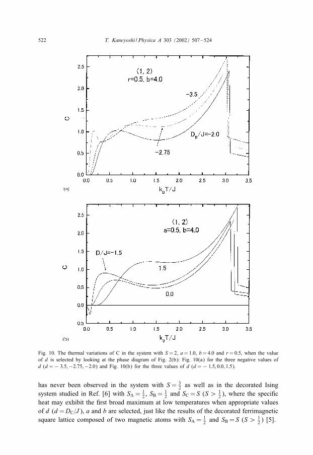
in the thermal variation of speci+c heat. Fig. 10 shows such typical results for theferrimagnetic system with S =2, r=0:5, a=1:0 and b=4:0, selecting some values ofd from Fig. 2(b). As shown in Fig. 10(a), the speci+c heat exhibits some characteristic


Fig. 8. The thermal variations of the speci+c heat C in the two ferrimagnetic systems corresponding toFigs. 3(a) and 3(b). Fig. 8(a) is obtained for the system with S = 3

2 , a=1:0, b=4:0 and r=0:5, when thethree values of d are selected. Fig. 8(b) is plotted for the two systems with S =2, a=1 and b=4:0, whenthe two values of r and d are selected from Fig. 1(b): d=− 1:05 and r=2:5 for the curve labeled andd=− 2:75 and r=0:5 for the curve labeled �.

features in the thermal variations, when we select the value of d smaller than d=−2:0.They are also observed in the thermal variation of C for the systems with S = 3

2 , asshown in Figs. 8(a) and 9. As depicted in Fig. 10(b), however, the thermal variationof C for the system with S =2 may exhibit an anomalous behavior in some regions


Fig. 9. The thermal variations of the speci+c heat C in the two ferrimagnetic systems corresponding toFigs. 4(a) and (b): Fig. 9(a) for Fig. 4(a) and Fig. 9(b) for Fig. 4(b).

between d= − 2:0 and −0:25, while for d¿ − 0:25 it also expresses the behaviorexpected for the system with S = 3

2 . The typical case showing the anomalous behaviorin C is plotted in the +gure, selecting the value of d=−1:5. It expresses some negativevalues in the very low temperature region, which implies that the system is physicallyin an unstable state. As depicted in Fig. 5(a), however, the temperature dependence of|M | in the ferrimagnetic system does not exhibit any anomalous behavior. Such a result


Fig. 10. The thermal variations of C in the system with S =2, a=1:0, b=4:0 and r=0:5, when the valueof d is selected by looking at the phase diagram of Fig. 2(b): Fig. 10(a) for the three negative values ofd (d=− 3:5;−2:75;−2:0) and Fig. 10(b) for the three values of d (d=− 1:5; 0:0; 1:5).

has never been observed in the system with S = 32 as well as in the decorated Ising

system studied in Ref. [6] with SA = 12 , SB =

12 and SC = S (S ¿ 1

2 ), where the speci+cheat may exhibit the +rst broad maximum at low temperatures when appropriate valuesof d (d=DC=J ), a and b are selected, just like the results of the decorated ferrimagneticsquare lattice composed of two magnetic atoms with SA = 1

2 and SB = S (S ¿ 12 ) [5].


4. Conclusions

In this work, we have studied the magnetic properties (phase diagram, spin–spin cor-relations, internal energy and speci+c heat) of the decorated ferrimagnetic Ising squarelattice composed of three magnetic atoms within the Bethe–Peierls approximation [9]on the basis of the di.erential operator technique. As shown in Fig. 2, we have foundthe possibility of two compensation points in the two systems with S = 3

2 and 2, evenwhen the spin directions of decorated B and C atoms are selected opposite to the spindirection of A atoms. The result is clearly in contrast to the results in the previouswork [6]. Furthermore, some interesting thermal variations of |M | not predicted in theNEeel theory have been obtained in Fig. 3.As shown in Figs. 8(b) and 9 and Fig. 10(a), we have found a new phenomenon in

the thermal variation of the speci+c heat, which expresses a second broad maximumwithin the intermediate region below TC in addition to the +rst broad maximum ob-tained at very low temperatures. The +rst broad maximum in C has also been observedin the exact results of the decorated isotropic Ising square lattice [5] as well as in theexact results of the decorated Ising chain [11]. As shown in Fig. 10(b), we have foundan anomalous behavior of the C in the system with S =2, d=−1:5, r=0:5, a=1:0 andb=4:0, in which it may exhibit some negative values in very low temperature region.The phenomenon has also been observed in other regions of d in the system with S =2.It implies that the system is physically in an unstable state. It may be better to takeanother state, such as the canted ferrimagnetic state due to the Dyialoshinski–Moriyainteraction, than the state of the present system. Anyway, it will give us an interestingproblem to study the phenomenon further, using a more sophisticated theoretical frame-work whether the unstable behavior of C in the system with S =2 is correct or not. Itis not clear physically why the +rst and second broad maximums may appear in thethermal variation of the speci+c heat of the system. Thus, as discussed in this work aswell as previous works [3–6], the decorated Ising systems with uniaxial anisotropiesmay be worth investigating once again, while the decorated Ising systems withoutany uniaxial anisotropy (except Ref. [10]) have been discussed in detail many yearsago [12].

References

[1] I. Syozi, H. Nakano, Prog. Theor. Phys. 13 (1955) 69.[2] L. NEeel, Ann. Phys. 3 (1948) 137.[3] T. Kaneyoshi, Physica A 229 (1996) 600.[4] T. Kaneyoshi, Physica A 237 (1997) 554.[5] A. Dakhama, Physica A 252 (1998) 225.[6] T. Kaneyoshi, J. Phys. Soc. Jpn. 70 (2001) 884.[7] T. Kaneyoshi, Acta Phys. Pol. A 195 (1993) 703.[8] R. Honmura, T. Kaneyoshi, J. Phys. C 12 (1979) 3979.[9] R. Honmura, Phys. Rev. B 30 (1984) 348.


[10] M. Hattori, Prog. Theor. Phys. 35 (1966) 600.[11] T. Kaneyoshi, Prog. Theor. Phys. 97 (1997) 407.[12] I. Syozi, in: C. Domb, M.S. Green (Eds.), Phase Transitions and Critical Phenomena, Vol. 1, Academic

Press, New York, 1972.[13] T.K. Hatwar, D.J. Genova, R.H. Victora, J. App. Phys. 75 (1994) 6858.[14] A. Herpin, Theorie du Magnetisme, Presses Universitaires de France, Saclay, 1968.

some characteristic properties of a decorated ferrimagnetic ising system

Documents