solving vision problems via filtering supplementary material
TRANSCRIPT

1
1. Experimental Results In our main paper, we provided experimental results for a number of vision-related inverse problems. 9is supplement provides additional details on the formulations used, as well as more extensive visual results for the experiments.
1.1. Disparity Super-resolution For our disparity super-resolution experiment, we use the dataset from [1], which is a subset of the Middlebury stereo dataset. We show visualizations of our 16× super-resolution disparity maps in Figure 4.
1.2. Optical Flow Estimation In our experiments, we use the color-gradient constancy model [2] instead of the brightness-constancy one [3]. In all cases, one can express the optical flow data fidelity term as
𝑑(𝐮) = ‖𝐇(𝐮 − 𝐮0) + 𝐳)‖22 (S1)
see (27) in our main paper. 9e color-constancy model gives us
𝐇 =
⎣⎢⎢⎡
𝐙/0 𝐙1
0
𝐙/2 𝐙1
2
𝐙/3 𝐙1
3⎦⎥⎥⎤
, 𝐳) =
⎣⎢⎢⎡
𝐳)0
𝐳)2
𝐳)3 ⎦
⎥⎥⎤
(S2)
in which 𝐙/,10,2,3 denotes the 𝑥- and the 𝑦-derivatives of the
target image in the 𝑅, 𝐺 and 𝐵 components, and 𝐳)0,2,3 are
the difference of the reference image from the target one, in the 𝑅, 𝐺 and 𝐵 image components. 9e gradient-constancy model on the other hand gives us the derivative data
𝐇 = [𝐙// 𝐙/1
𝐙1/ 𝐙11] , 𝐳) = [𝐳/)
𝐳1)] (S3)
in which 𝐙//, 𝐙/1 and 𝐙11 are the second-order derivatives of the target image, and 𝐳/) and 𝐳1) are the difference of the first-order differences of the reference image from the target ones. When the gradient constancy model is applied on each of the color channels, we obtain
𝐇 =
⎣⎢⎢⎢⎢⎢⎢⎡
𝐙//0 𝐙/1
0
𝐙1/0 𝐙11
0
𝐙//2 𝐙/1
2
𝐙1/2 𝐙11
2
𝐙//3 𝐙/1
3
𝐙1/3 𝐙11
3 ⎦⎥⎥⎥⎥⎥⎥⎤
, 𝐳) =
⎣⎢⎢⎢⎢⎢⎢⎡
𝐳/)0
𝐳1)0
𝐳/)2
𝐳1)2
𝐳/)3
𝐳1)3 ⎦
⎥⎥⎥⎥⎥⎥⎤
(S4)
in which we define the sub-matrices of 𝐇 and 𝐳) similarly to before. Revaud et al. [4] use a weighted combination of two data terms 𝑑(𝐮) based on (S2) and (S4). 9is combination can be understood as forming new 𝐇 and 𝐳) by stacking the ones in (S2) and (S4). When the two data terms are combined using equal weights, the inverse covariance matrix 𝐇∗𝐇 becomes
𝐙 = [∑𝐙∗/𝐙∗/ ∑𝐙∗/𝐙∗1
∑𝐙∗/𝐙∗1 ∑𝐙∗1𝐙∗1] , (S5)
and the transformed signal is
𝐇†𝐳 = [∑𝐙∗/𝐳∗)∑𝐙∗1𝐳∗)
] , (S6)
cf. (27) in our main paper. In (S5)–(S6), the summations are over the three color channels for each of the 0th, and the 1st partial derivatives of the image. Figure 1 visualizes our flow estimates.
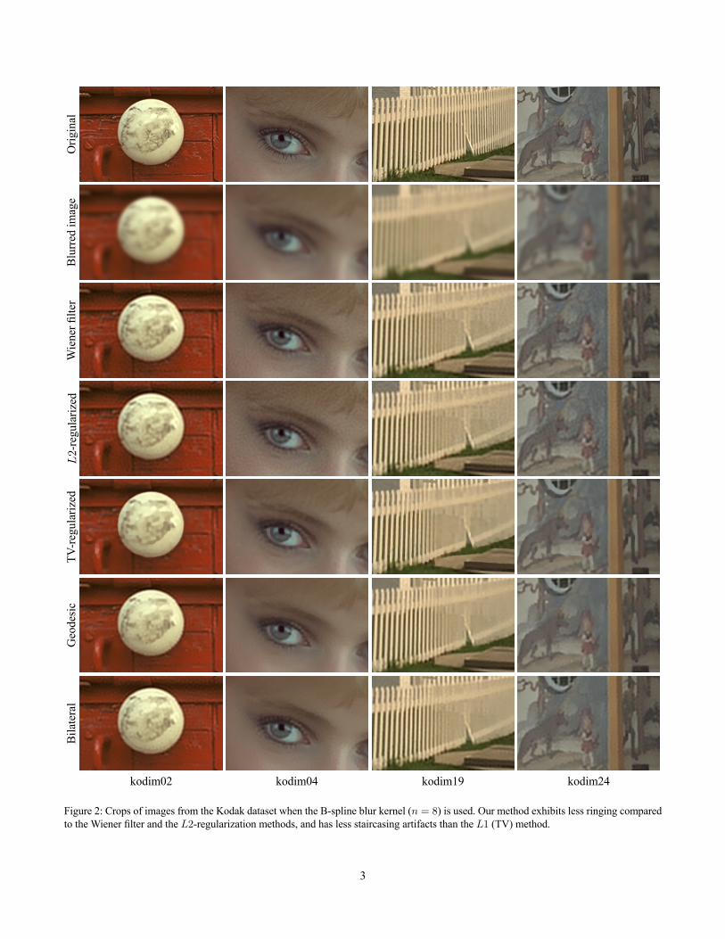
1.3. Image Deblurring Figure 2 provides crops of the deblurred images from the the Kodak dataset [2], produced by different algorithms. We optimize the algorithm parameters for the different methods (Wiener, 𝐿2, and TV) via grid search. 9e Wiener filter uses a uniform image power spectrum model. Note the use of the bilateral filter is not optimal for de-noising as pointed out by Buades et al. [5], who demonstrate the advantages of patch-based filtering (nonlocal means denoising) over pixel-based filtering (bilateral filter). Our deblurring results are based on the bilateral filter, but one is free to use the non-local means filter (or any other filter) for the de-noising operator 𝐀.
Solving Vision Problems via Filtering Supplementary Material
Sean I. Young1 Aous T. Naman2 Bernd Girod1 David Taubman2
[email protected] [email protected] [email protected] [email protected]
1Stanford University 2University of New South Wales

2
alle
y_1
(001
0)
Blur
red
imag
e
cave
_4 (0
038)
bam
boo_
2 (0
038)
G
eode
sic
band
age_
1 (0
003)
band
age_
2 (0
041)
Ground truth Initial flow Geodesic Bilateral
Figure 1: Optical flow (top rows) and the corresponding flow error (bottom rows) produced using the geodesic and the bilateral variants of our method. Whiter pixels correspond to smaller flow vectors.
3
Orig
inal
Blur
red
imag
e
Wie
ner fi
lter
𝐿 2-re
gula
rized
TV-re
gula
rized
Geo
desic
Bila
tera
l
kodim02 kodim04 kodim19 kodim24
Figure 2: Crops of images from the Kodak dataset when the B-spline blur kernel (𝑛 = 8) is used. Our method exhibits less ringing compared to the Wiener filter and the 𝐿2-regularization methods, and has less staircasing artifacts than the 𝐿1 (TV) method.

4
Art
16×
Book
s 16 ×
Möb
ius 1
6×
Reference image Ground truth disparity Low-resolution disparity Our disparity (geodesic) Our disparity (bilateral)
Figure 4: 9e 16× super-resolution disparity maps produced using the geodesic and the bilateral variants of our method for the 1088 × 1376 scenes Art, Books, and Möbius used in [1]. Best viewed online by zooming in.
2. Possible Limitations In Section 4 of our paper, we discussed that (14a) is valid only when (14a) matrix (𝐂 + 𝜆𝐋)−1 has a low-pass spectral response. We show this in Figure 4 (left) for the case where 𝜆 = 1 and 𝐂 = 𝐈. Since 𝐂 + 𝜆𝐋 is Sinkhorn-normalized, it has a high-pass spectral response 𝐼 + 𝜆�̂�, ranging from 1 to 2. As a consequence, the inverse filter response (𝐼 + 𝜆𝐿)−1̂ ranges from 1 down to 0.5. We can approximate such a filter response as a sum of low-pass and all-pass responses. In our
context, an approximation of 𝐮opt = (𝐂 + 𝜆𝐋)−1𝐂𝐳 can be obtained using a convex combination of 𝐂𝐳 and a low-pass-filtered version 𝐀𝐂𝐳 of it. On the other hand, if 𝐼 + 𝜆�̂� is a low-pass response. In this case, the inverse response (shown in Figure 4, right) is high-pass, and the solution 𝐮opt cannot be approximated as a convex combination of 𝐂𝐳 and a low-pass-filtered version of it. In practice, we can still use (14b) to solve the transformed problem.
References [1] Jaesik Park, Hyeongwoo Kim, Yu-Wing Tai, Michael S.
Brown, and In So Kweon. High quality depth map upsampling for 3D-TOF cameras. In ICCV, 2011.
[2] Nils Papenberg, Andrés Bruhn, 9omas Brox, Stephan Didas, and Joachim Weickert. Highly accurate optic flow computation with theoretically justified warping. Int. J. Comput. Vis., 67(2):141–158, 2006.
[3] Berthold K. P. Horn and Brian G. Schunck. Determining optical flow. Artif. Intell., 17(1):185–203, 1981.
[4] Jerome Revaud, Philippe Weinzaepfel, Zaid Harchaoui, and Cordelia Schmid. EpicFlow: Edge-preserving interpolation of correspondences for optical flow. In CVPR, 2015.
[5] Antoni Buades, Bartomeu Coll, and Jean-Michel Morel. A non-local algorithm for image denoising. In CVPR, 2005.
Figure 3. 9e frequency response (𝐶 + 𝜆𝐿)−1̂ can be expressed as a sum of low-pass response 𝐴 ̂and an all-pass one 𝐼 ̂only when the response (𝐶 + 𝜆𝐿)−1̂ is low-pass-like (left). Shown for 𝜆 = 1.
𝐼 + 𝜆�̂�
(𝐼 + 𝜆𝐿)−1̂ 𝐴 ̂
𝐼 ̂
𝐼 + 𝜆�̂�
(𝐼 + 𝜆𝐿)−1̂
𝐼 ̂