Frequency Domain FilteringFrequency Domain Filtering

Correspondence between Spatial and Frequency Filtering

Fourier TransformBrief IntroductionSampling Theoryp g y2‐D Discrete Fourier Transform

Convolution

Spatial AliasingSpatial Aliasing

Frequency domain filtering fundamentals

ApplicationsppImage smoothingImage sharpeningSelective filteringSelective filtering

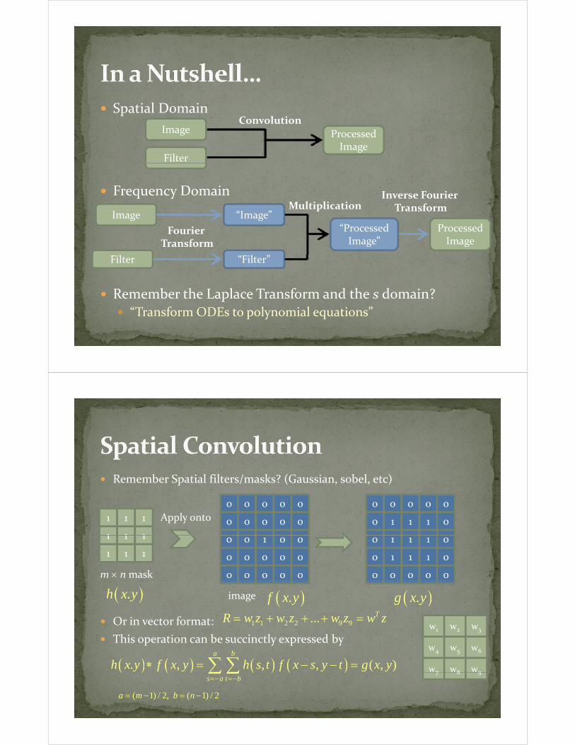
Spatial DomainC l ti

Image

Filter

Processed Image

Convolution

Frequency DomainMultiplication

Inverse Fourier Transform

ImageProcessed Image

“Image”

Fourier Transform

“Processed Image”

Multiplication Transform

Remember the Laplace Transform and the s domain?

Filter “Filter”

p“Transform ODEs to polynomial equations”

Remember Spatial filters/masks? (Gaussian, sobel, etc)

1 1 1

1 1 1

0 0 0

0 0 0

0 0

0 0Apply onto

0 0 0

0 1 1

0 0

1 0

1 1 1

1 1 1

m × n mask

0 0 1 0 0

0 0

0 0

0 0 0

0 0 0

0 1 1 1 0

0 1

0 0

1 1 0

0 0 0

Or in vector format:

image( ).h x y ( ).f x y ( ).g x y

1 1 2 2 9 9... TR w z w z w z w z= + + + =w w w

This operation can be succinctly expressed by

( ) ( ) ( ) ( ). , , , ( , )a b

h x y f x y h s t f x s y t g x y∗ = − − =∑ ∑

w1 w2 w3

w4 w5 w6

w7 w8 w9( ) ( ) ( ) ( )

s a t b=− =−∑ ∑

( 1) / 2, ( 1) / 2a m b n= − = −

7 8 9

Any periodic function can be represented by a sum of sines and cosines: Fourier Series

Extension to non‐periodic functions : Fourier T fTransform

Operation that transforms one complex‐valued function of a real variable into anotherfunction of a real variable into another

Continuous FT

Discrete FT

Single/Multivariate FT

Representing complex numbers:g

C R jI= +

( ) 2 2cos sinC C j C R Iθ θ= + = +( )cos sin ,C C j C R Iθ θ= + = +

, cos sinj jC C e e jθ θ θ θ= = +

Fourier Series:

2 2/2

/2

1( ) , ( )

n nTj t j t

T Tn n T

n

f t c e c f t e dtT

π π∞ −

−=−∞

= =∑ ∫C R jI= +

Continuous single variate:g

{ } ( ) 2( ) ( ) j tf t F f t e dtπμμ∞ −

−∞ℑ = = ∫

Conversely, Inverse Fourier Transform:

Fourier Transform Pair

( ){ } ( )1 2( ) j tf t F F e dtπμμ μ∞−

−∞= ℑ = ∫

Using Euler’s formula,

( ) ( ) ( )( ) cos 2 sin 2F f t t j t dtμ πμ πμ∞

= −⎡ ⎤⎣ ⎦∫( ) ( ) ( )( ) cos 2 sin 2F f t t j t dtμ πμ πμ−∞

= −⎡ ⎤⎣ ⎦∫

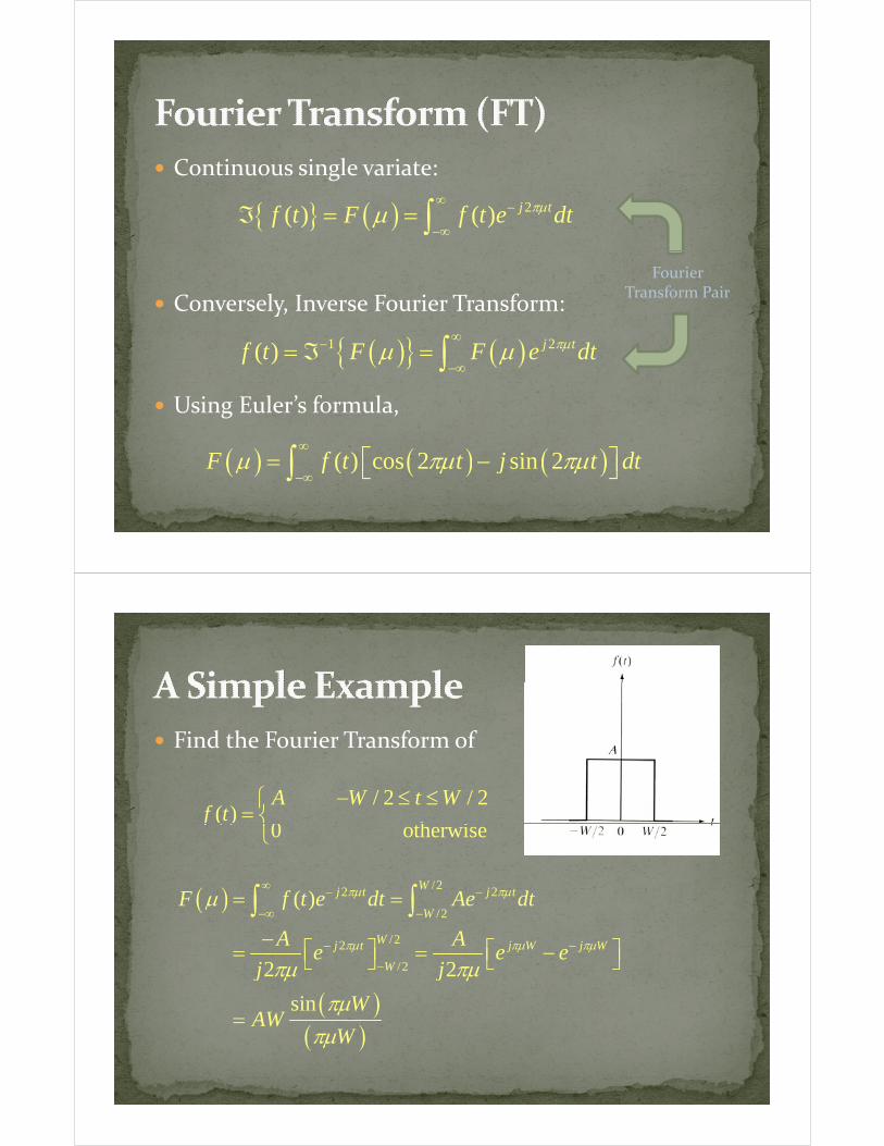
Find the Fourier Transform of 

/ 2 / 2( )

0 h i

A W t Wf t

− ≤ ≤⎧= ⎨⎩

( )0 otherwise

f ⎨⎩

( )/22 2( )

Wj t j tF f t dt A dtπμ πμ∞ − −∫ ∫( ) 2 2

/2

/22

/2

( )

2 2

j t j t

W

Wj t j W j W

W

F f t e dt Ae dt

A Ae e e

j j

πμ πμ

πμ πμ πμ

μ−∞ −

− −

= =

− ⎡ ⎤ ⎡ ⎤= = −⎣ ⎦ ⎣ ⎦

∫ ∫

( )( )

/22 2

sin

Wj j

WAW

W

πμ πμπμ

πμ

−⎣ ⎦ ⎣ ⎦

=( )Wπμ

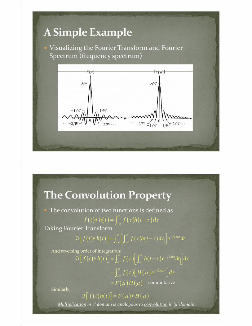
Visualizing the Fourier Transform and Fourier gSpectrum (frequency spectrum)

The convolution of two functions is defined as

Taking Fourier Transform

( ) ( ) ( ) ( )f t h t f h t dτ τ τ∞

−∞∗ = −∫

⎡ ⎤

And reversing order of integration:

( ) ( ) ( ) ( ) 2j tf t h t f h t d e dtπμτ τ τ∞ ∞ −

−∞ −∞

⎡ ⎤ℑ ∗ = −⎡ ⎤⎣ ⎦ ⎢ ⎥⎣ ⎦∫ ∫

⎡ ⎤( ) ( ) ( ) ( )

( ) ( )

2

2

j t

j

f t h t f h t e dt d

f H e d

πμ

πμτ

τ τ τ

τ μ τ

∞ ∞ −

−∞ −∞

∞ −

⎡ ⎤ℑ ∗ = −⎡ ⎤⎣ ⎦ ⎢ ⎥⎣ ⎦

⎡ ⎤= ⎣ ⎦

∫ ∫

∫

Similarly: 

( ) ( )( ) ( )

f

F H

μ

μ μ−∞ ⎣ ⎦

=∫

commutative

( ) ( ) ( ) ( )f h F Hℑ⎡ ⎤⎣ ⎦( ) ( ) ( ) ( )f t h t F Hμ μℑ = ∗⎡ ⎤⎣ ⎦Multiplication in ‘t’ domain is analogous to convolution in ‘μ’ domain

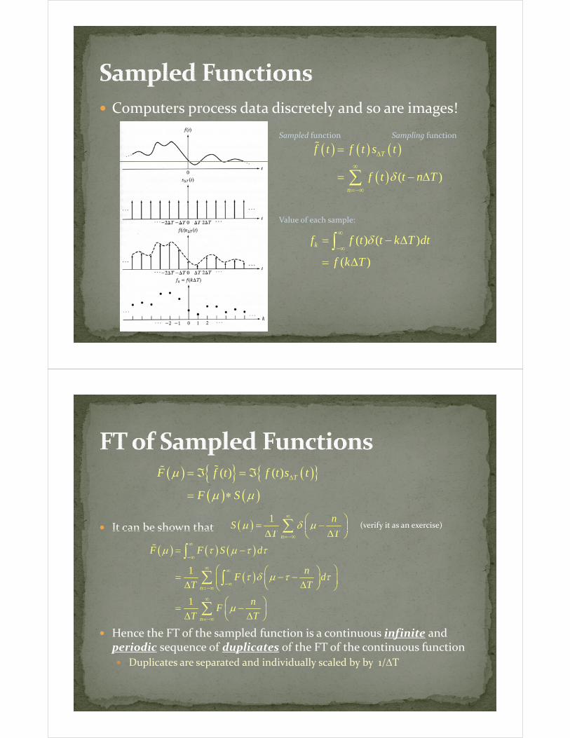
Computers process data discretely and so are images!g

( ) ( ) ( )Tf t f t s tΔ=Sampled function Sampling function

( ) ( )n

f t t n Tδ∞

=−∞

= − Δ∑

Value of each sample:

( ) ( )kf f t t k T dtδ∞

−∞= − Δ∫

( )f k T= Δ

( ) { } ( ){ }( ) ( ) TF f t f t s tμ Δ= ℑ = ℑ

It can be shown that

( ) ( )F Sμ μ= ∗

( ) 1 nS

T Tμ δ μ

∞ ⎛ ⎞= −⎜ ⎟Δ Δ⎝ ⎠∑ (verify it as an exercise)It can be shown that ( )

nT Tμ μ

=−∞⎜ ⎟Δ Δ⎝ ⎠

∑( ) ( ) ( )

( )1

F F S d

nF d

μ τ μ τ τ

τ δ μ τ τ

∞

−∞

∞ ∞

= −

⎛ ⎞⎛ ⎞⎜ ⎟⎜ ⎟

∫

∑ ∫ ( )

1

n

n

F dT T

nF

T T

τ δ μ τ τ

μ

−∞=−∞

∞

=−∞

= − −⎜ ⎟⎜ ⎟Δ Δ⎝ ⎠⎝ ⎠⎛ ⎞= −⎜ ⎟Δ Δ⎝ ⎠

∑ ∫

∑Hence the FT of the sampled function is a continuous infinite and periodic sequence of duplicates of the FT of the continuous function

Duplicates are separated and individually scaled by by 1/ΔT

⎝ ⎠

p p y y y /

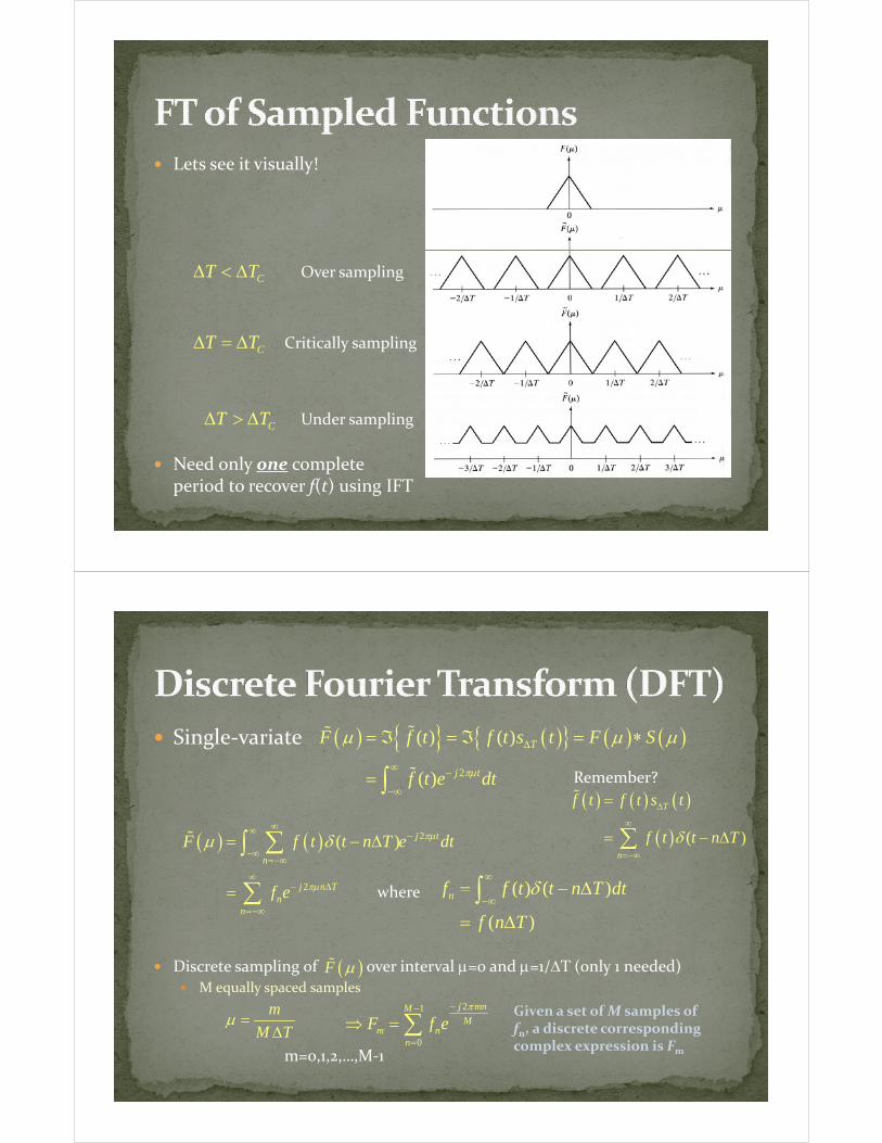
Lets see it visually!

Over samplingCT TΔ < Δ

Critically samplingCT TΔ = Δ

N d  l   l t  

Under samplingCT TΔ > Δ

Need only one complete period to recover f(t) using IFT

Single‐variate ( ) { } ( ){ } ( ) ( )( ) ( ) TF f t f t s t F Sμ μ μΔ= ℑ = ℑ = ∗{ }2( ) j tf t e dtπμ∞ −

−∞= ∫

( ) ( ) ( )Tf t f t s tΔ=Remember?

( ) ( )n

f t t n Tδ∞

=−∞

= − Δ∑( ) ( ) 2

2

( ) j t

n

j n T

F f t t n T e dt

f e

πμ

πμ

μ δ∞∞ −

−∞=−∞

∞− Δ

= − Δ

=

∑∫

∑ where ( ) ( )f f t t n T dtδ∞

= − Δ∫

Di   li   f              i l    d  /ΔT ( l     d d)

jn

n

f e μ

=−∞

= ∑ where ( ) ( )

( )

nf f t t n T dt

f n T

δ−∞

Δ

= Δ∫

( )Discrete sampling of            over interval μ=0 and μ=1/ΔT (only 1 needed)M equally spaced samples

( )F μ

m

M Tμ =

Δ

21 j mnMM

m nF f eπ−−

⇒ = ∑Given a set of M samples of f , a discrete corresponding M TΔ

0m n

n

f=∑

m=0,1,2,…,M‐1

fn, a discrete corresponding complex expression is Fm 

Conversely given a set of Fm discrete data points, a g m

sample set of fn can be recovered.211 j mnMM

n mf F eM

π−

= ∑IDFT: DFT:

21

0

j mnMM

m nF f eπ−−

= ∑ m,n=0,1,2,…,M‐1

( )

0mM =∑

0n=

Discrete Fourier Transform Pair

In image (spatial) processing, the more natural and widely used expression is:

( ) ( )21

0

1 j uxMM

u

f x F u eM

π−

=

= ∑ ( ) ( )21

0

j uxMM

x

F u f x eπ−−

=

= ∑

Image Processing: x y are spatial variables and u v are ‘spatial frequency’ variables

u,x=0,1,2,…,M‐1

Image Processing: x,y are spatial variables and u,v are  spatial frequency  variables

Signal Processing: t is a temporal variable and μ is a frequency variable

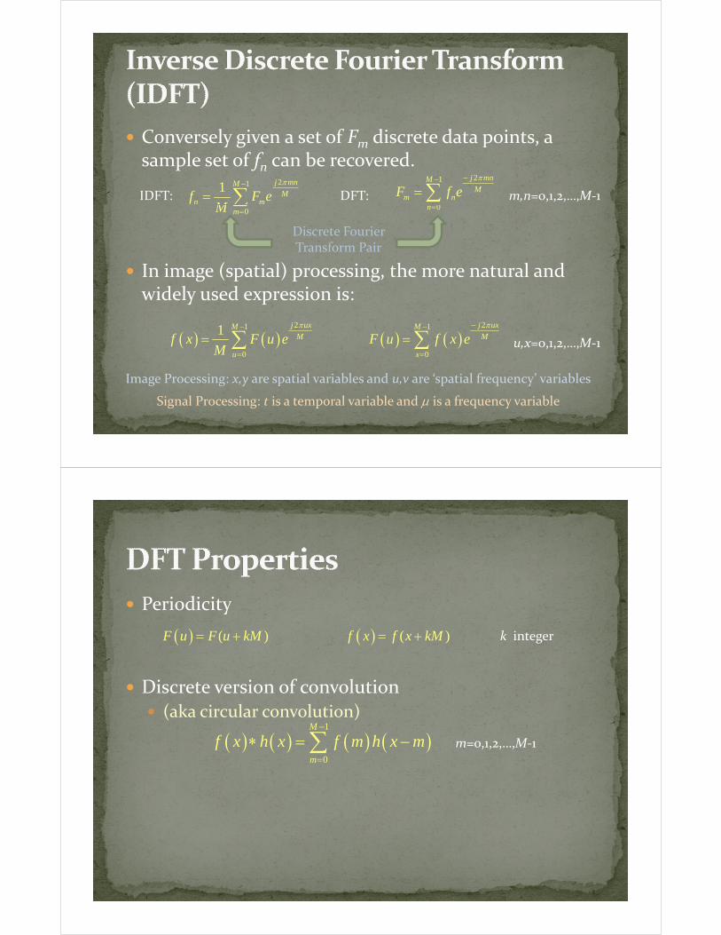
Periodicity

( ) ( )F u F u kM= + ( ) ( )f x f x kM= + k  integer

Discrete version of convolution (aka circular convolution)

1M −

( ) ( ) ( ) ( )1

0

M

m

f x h x f m h x m=

∗ = −∑ m=0,1,2,…,M‐1

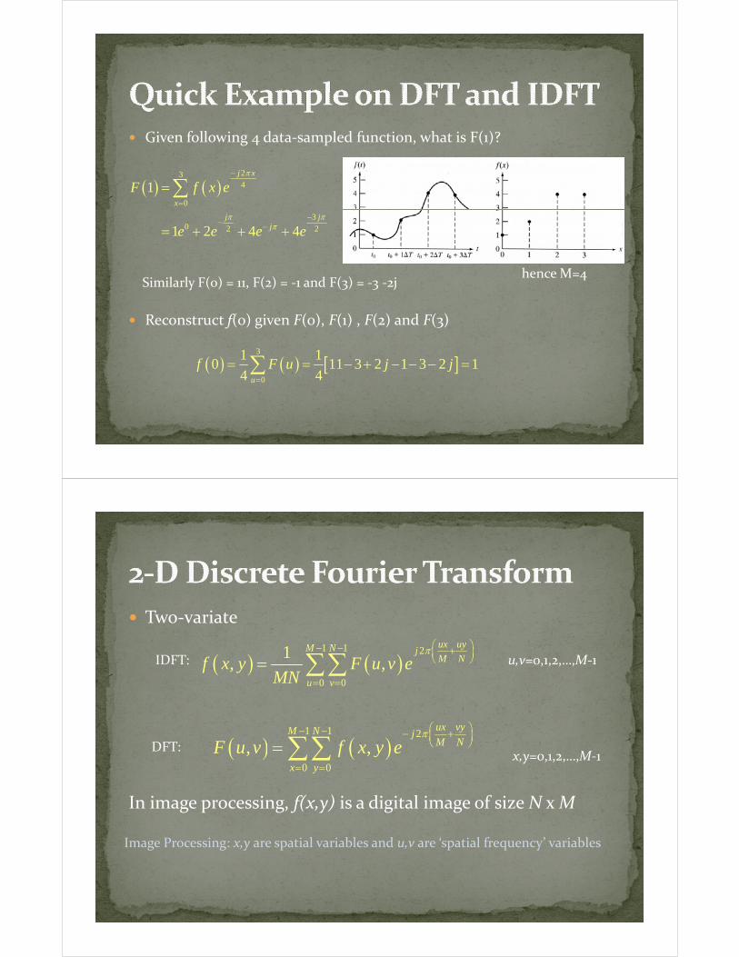
Given following 4 data‐sampled function, what is F(1)?

( ) ( )234

0

1j x

x

F f x eπ−

=

=∑

h  M

30 2 21 2 4 4

j jje e e e

π ππ

−− −= + + +

Reconstruct f(0) given F(0), F(1) , F(2) and F(3)

hence M=4Similarly F(0) = 11, F(2) = ‐1 and F(3) = ‐3 ‐2j

f( ) g ( ) ( ) ( ) (3)

( ) ( ) [ ]3

0

1 10 11 3 2 1 3 2 1

4 4u

f F u j j=

= = − + − − − =∑

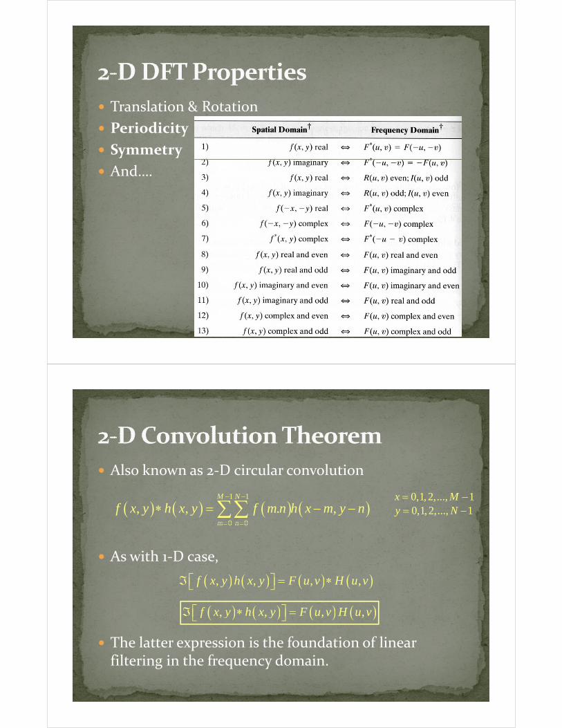
Two‐variate

IDFT: ( ) ( )1 1 2

0 0

1, ,

ux uyM N jM N

u v

f x y F u v eMN

π ⎛ ⎞− − +⎜ ⎟⎝ ⎠

= =

= ∑∑ u,v=0,1,2,…,M‐1

DFT: ( ) ( )1 1 2

ux vyM N jM NF u v f x y e

π ⎛ ⎞− − − +⎜ ⎟⎝ ⎠= ∑∑

In image processing  f(x y) is a digital image of size N x M

DFT: ( ) ( )0 0

, ,x y

F u v f x y e ⎝ ⎠

= =

= ∑∑ x,y=0,1,2,…,M‐1

In image processing, f(x,y) is a digital image of size N x M

Image Processing: x,y are spatial variables and u,v are ‘spatial frequency’ variables

Translation & Rotation

Periodicity

Symmetry

And….

Also known as 2‐D circular convolution

( ) ( ) ( ) ( )1 1

0 0

, , . ,M N

m n

f x y h x y f m n h x m y n− −

= =

∗ = − −∑∑0,1,2,..., 1x M= −0,1,2,..., 1y N= −

As with 1‐D case,

0 0m n= =

( ) ( ) ( ) ( ), , , ,f x y h x y F u v H u vℑ = ∗⎡ ⎤⎣ ⎦

( ) ( ) ( ) ( )f x y h x y F u v H u vℑ ∗ =⎡ ⎤⎣ ⎦

The latter expression is the foundation of linear filt i  i  th  f  d i

( ) ( ) ( ) ( ), , , ,f x y h x y F u v H u vℑ ∗ =⎡ ⎤⎣ ⎦

filtering in the frequency domain.

Before foraging into frequency domain filtering, lets do a quick digress into aliasing in digital imaging

What is Aliasing?High frequency components “masquerading” as lower High frequency components  masquerading  as lower frequencies

Temporal Aliasing

Pertains to time intervals between images in a sequencePertains to time intervals between images in a sequence

The “wagon wheel” effect

Capturing frame rate too low

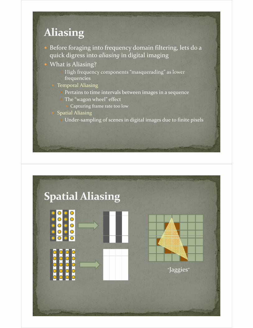
Spatial AliasingSpatial Aliasing

Under‐sampling of scenes in digital images due to finite pixels

“Jaggies”

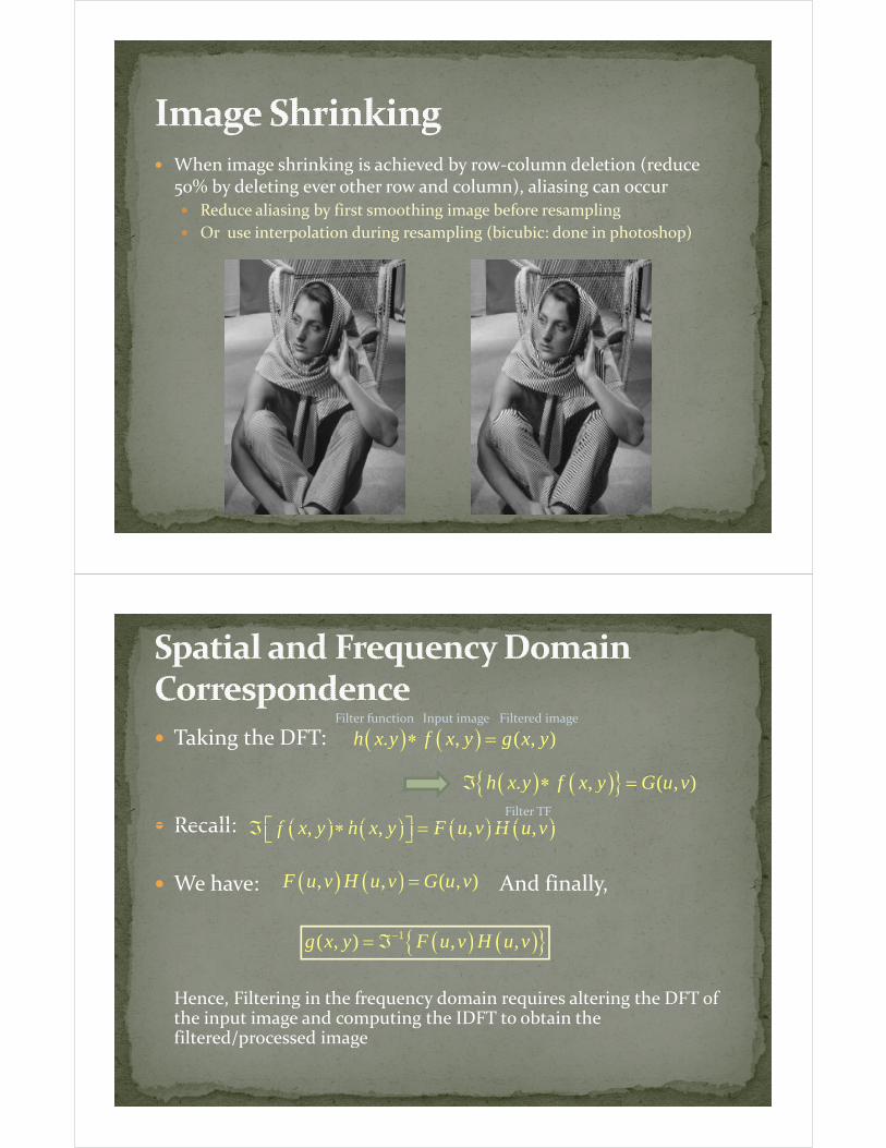
When image shrinking is achieved by row‐column deletion (reduce % b  d l i     h     d  l )   li i    50% by deleting ever other row and column), aliasing can occur

Reduce aliasing by first smoothing image before resampling

Or  use interpolation during resampling (bicubic: done in photoshop) 

Taking the DFT: ( ) ( ). , ( , )h x y f x y g x y∗ =Input imageFilter function Filtered image

Recall:

( ) ( ){ }. , ( , )h x y f x y G u vℑ ∗ =

( ) ( ) ( ) ( )f h F Hℑ ∗⎡ ⎤⎣ ⎦Filter TF

Recall:

We have:                                            And finally,

( ) ( ) ( ) ( ), , , ,f x y h x y F u v H u vℑ ∗ =⎡ ⎤⎣ ⎦

( ) ( ), , ( , )F u v H u v G u v= y

( ) ( ){ }1( , ) , ,g x y F u v H u v−= ℑ

Hence, Filtering in the frequency domain requires altering the DFT of the input image and computing the IDFT to obtain the filtered/processed imagefiltered/processed image

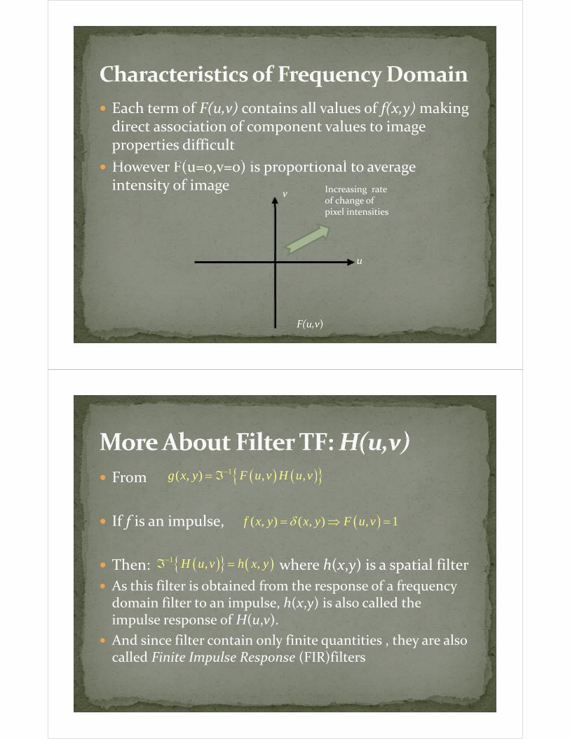
Each term of F(u,v) contains all values of f(x,y) making f y gdirect association of component values to image properties difficult

H  F( ) i   i l     However F(u=0,v=0) is proportional to average intensity of image

v Increasing  rate of change of pixel intensities

u

F(u,v)

From ( ) ( ){ }1( , ) , ,g x y F u v H u v−= ℑ

If f is an impulse, ( )( , ) ( , ) , 1f x y x y F u vδ= ⇒ =

Then:  where h(x,y) is a spatial filter( ){ } ( )1 , ,H u v h x y−ℑ =

As this filter is obtained from the response of a frequency domain filter to an impulse, h(x,y) is also called the impulse response of H(u v)impulse response of H(u,v).

And since filter contain only finite quantities , they are also called Finite Impulse Response (FIR)filters

Edges and noise contribute to the high‐frequency g gcomponents of an image’s FT

Smoothing or blurring is achieved by high‐frequency i  attenuation 

Low‐Pass FiltersIdeal lowpass filters (sharp)Ideal lowpass filters (sharp)

Butterworth lowpass filter

Gaussian Lowpass filter (smooth)p

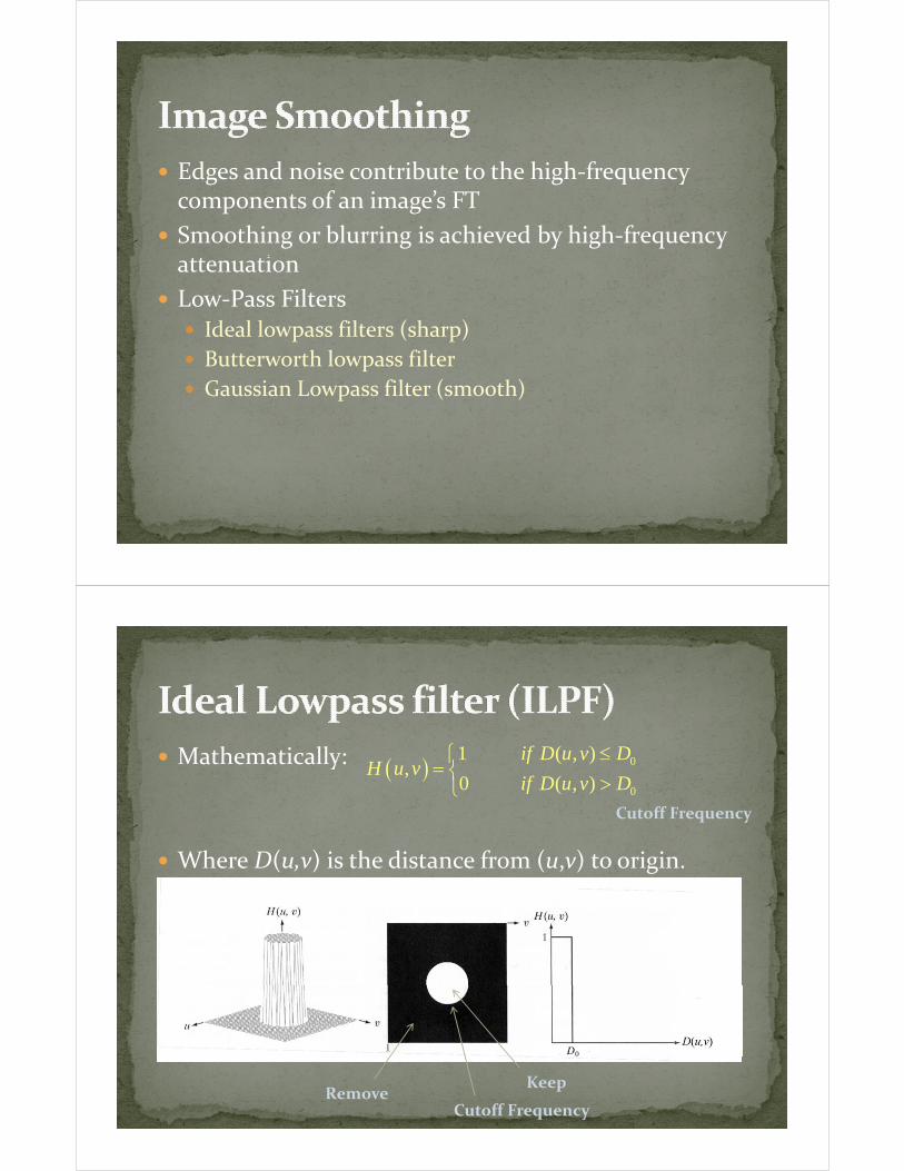
Mathematically: ( ) 01 ( , )if D u v DH u v

≤⎧= ⎨( )

0

,0 ( , )

H u vif D u v D

= ⎨ >⎩Cutoff Frequency

Where D(u,v) is the distance from (u,v) to origin.

RemoveKeep

Cutoff Frequency

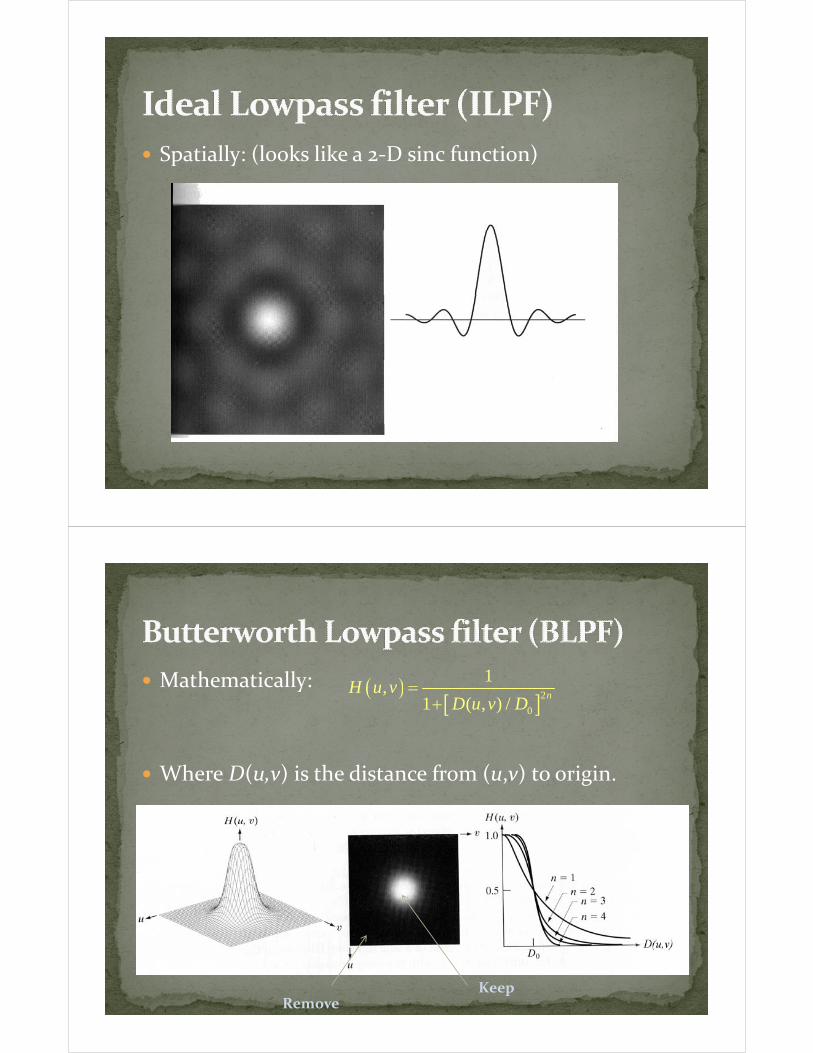
Spatially: (looks like a 2‐D sinc function)

Mathematically: ( ) 2

1,H u v =( )

[ ]20

,1 ( , ) /

nH u vD u v D+

Where D(u,v) is the distance from (u,v) to origin.

RemoveKeep

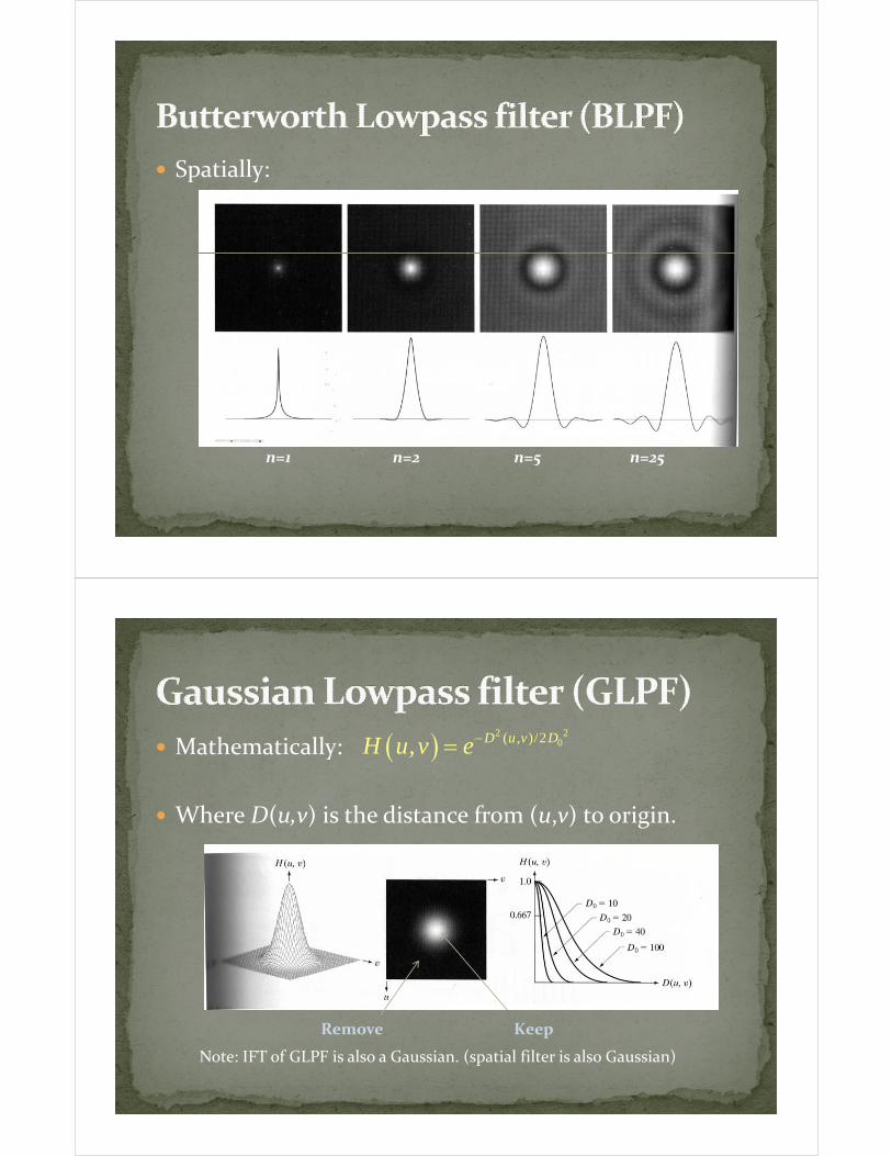
Spatially:

n=1 n=2 n=5 n=25

Mathematically: ( ) 2 20( , )/2, D u v DH u v e−=

Where D(u,v) is the distance from (u,v) to origin.

( )

Remove Keep

Note: IFT of GLPF is also a Gaussian. (spatial filter is also Gaussian) 

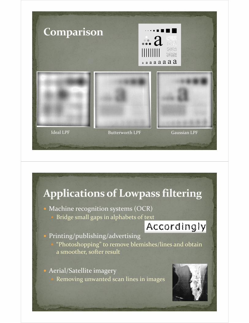
Ideal LPF Butterworth LPF Gaussian LPF

Machine recognition systems (OCR)gBridge small gaps in alphabets of text

Printing/publishing/advertising“Photoshopping” to remove blemishes/lines and obtain a smoother  softer resulta smoother, softer result

Aerial/Satellite imageryAerial/Satellite imageryRemoving unwanted scan lines in images

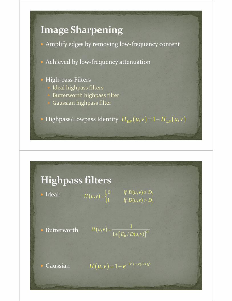
Amplify edges by removing low‐frequency contentg g

Achieved by low‐frequency attenuation

High‐pass FiltersIdeal highpass filters

Butterworth highpass filter

Gaussian highpass filterGaussian highpass filter

Highpass/Lowpass Identity ( ) ( ), 1 ,HP LPH u v H u v= −g p / p y ( ) ( ), ,HP LP

Ideal: ( ) 00 ( , ),

if D u v DH u v

≤⎧= ⎨( )

0

,1 ( , )if D u v D⎨ >⎩

Butterworth ( )[ ]2

1,

1 / ( )nH u v

D D u v=

+[ ]01 / ( , )D D u v+

Gaussian ( ) 2 20( , )/2, 1 D u v DH u v e−= −

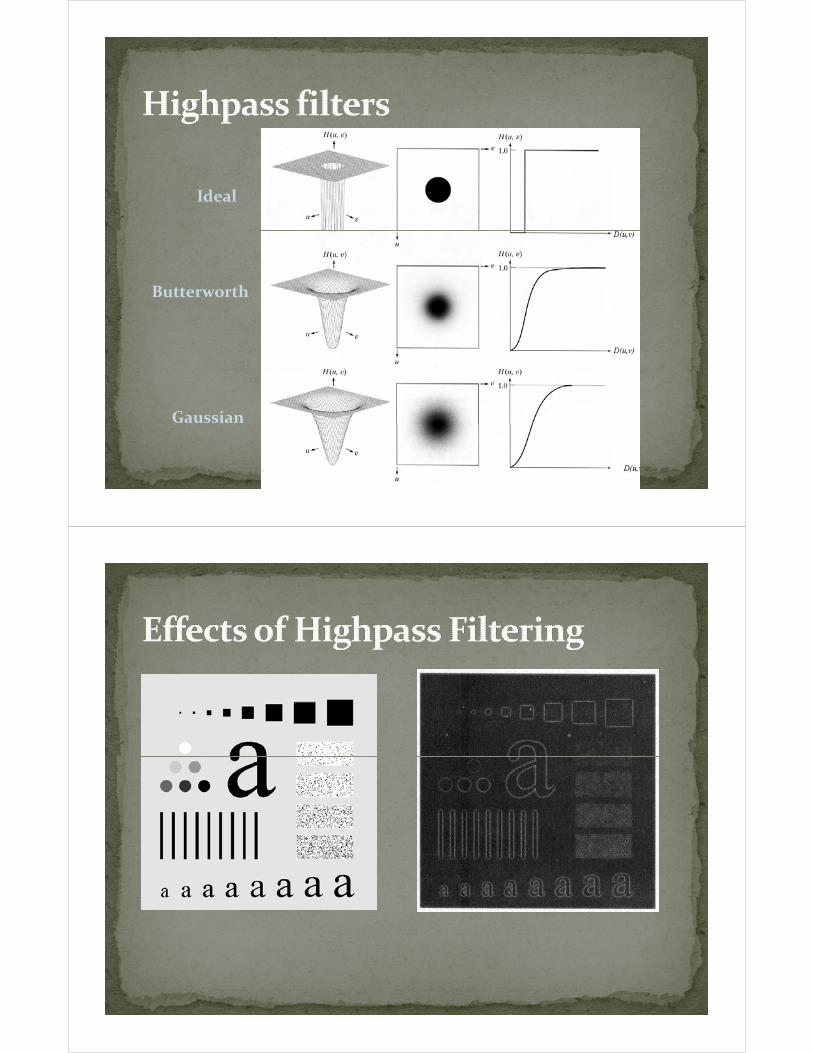
Ideal

ButterworthButterworth

Gaussian

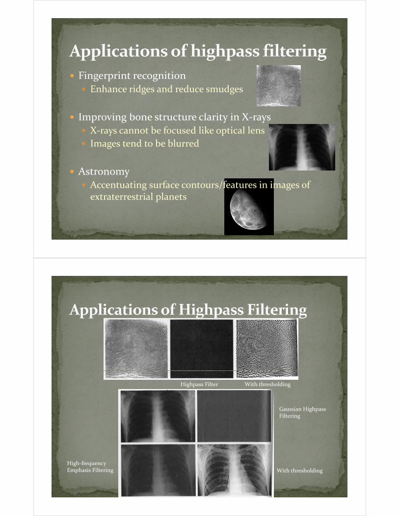
Fingerprint recognitiong gEnhance ridges and reduce smudges

I i  b     l i  i  XImproving bone structure clarity in X‐raysX‐rays cannot be focused like optical lens

Images tend to be blurredImages tend to be blurred

AstronomyyAccentuating surface contours/features in images of extraterrestrial planets

Highpass Filter With thresholding

Gaussian HighpassFiltering

High‐frequency

With thresholding

g q yEmphasis Filtering

Process specific bands / small regions of frequenciesg

Bandreject filters / Bandpass filtersIdeal filters

Butterworth filter

Gaussian filter

Notch filtersNotch filtersIdeal filters

Butterworth filter

Gaussian filter

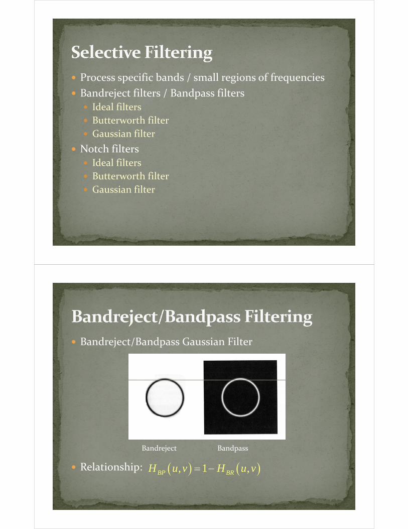
Bandreject/Bandpass Gaussian Filterj

d d

Relationship: ( ) ( ), 1 ,BP BRH u v H u v= −

Bandreject Bandpass

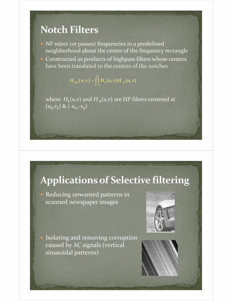
NF reject (or passes) frequencies in a predefined neighborhood about the center of the frequency rectangle

Constructed as products of highpass filters whose centers have been translated to the centers of the notcheshave been translated to the centers of the notches

( )1

, ( , ) ( , )Q

NR k kk

H u v H u v H u v−= ∏

where  Hk(u,v) and H‐k(u,v) are HP filters centered at 

1k−

(uk,vk) & (‐uk,‐vk)

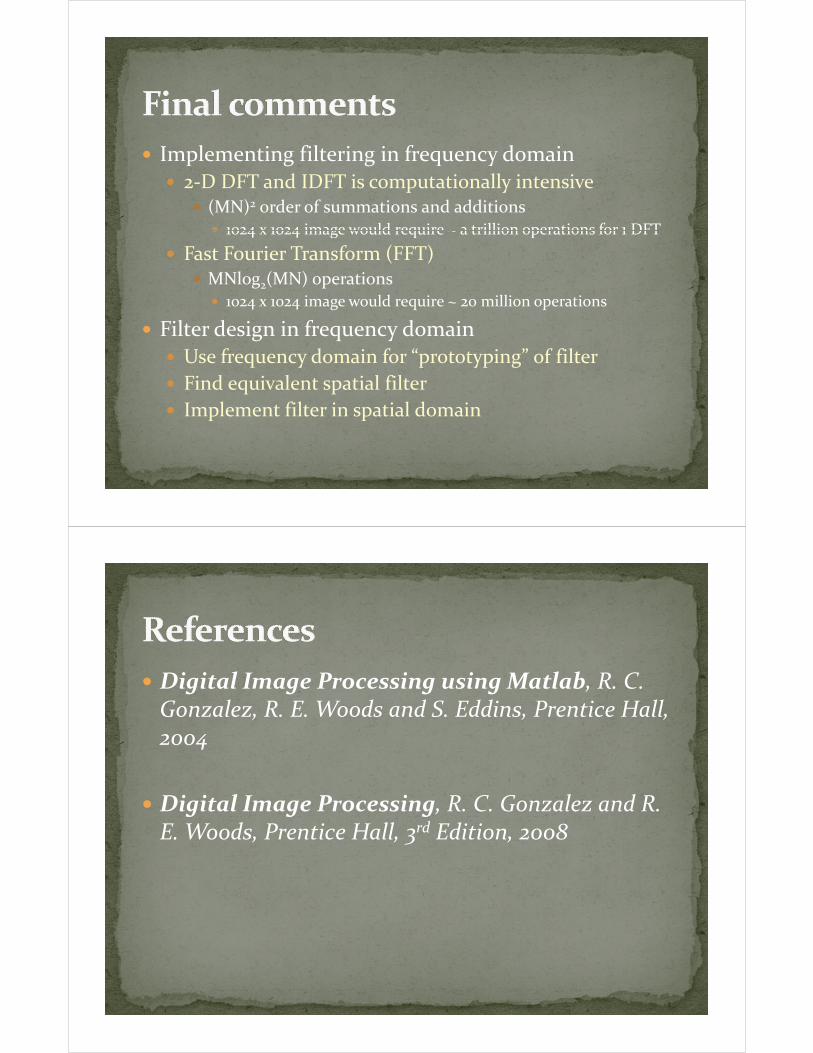
Reducing unwanted patterns in gscanned newspaper images

Isolating and removing corruption caused by AC signals (vertical sinusoidal patterns)sinusoidal patterns)

Implementing filtering in frequency domaing g2‐D DFT and IDFT is computationally intensive

(MN)2 order of summations and additions

1024 x 1024 image would require ~ a trillion operations for 1 DFT1024 x 1024 image would require ~ a trillion operations for 1 DFT

Fast Fourier Transform (FFT)MNlog2(MN) operations

     i   ld  i       illi   i1024 x 1024 image would require ~ 20 million operations

Filter design in frequency domainUse frequency domain for “prototyping” of filterUse frequency domain for  prototyping  of filter

Find equivalent spatial filter

Implement filter in spatial domain

Digital Image Processing using Matlab, R. C. g g g gGonzalez, R. E. Woods and S. Eddins, Prentice Hall, 2004

Digital Image Processing, R. C. Gonzalez and R. dE. Woods, Prentice Hall, 3rd Edition, 2008