Solving the p-Center Problem with Tabu Search andVariable Neighborhood Search

Nenad MladenovicService de Mathematiques de la Gestion, Universite Libre de Bruxelles, Brussels, Belgium; GERAD and HECMontreal, 3000, ch. de la Cote-Sainte-Catherine, Montreal, Quebec, Canada H3T 2A7

Martine LabbeService de Mathematiques de la Gestion, Universite Libre de Bruxelles, Belgium

Pierre HansenGERAD and HEC Montreal, 3000, ch. de la Cote-Sainte-Catherine, Montreal, Quebec, Canada H3T 2A7

The p-Center problem consists of locating p facilitiesand assigning clients to them in order to minimize themaximum distance between a client and the facility towhich he or she is allocated. In this paper, we present abasic Variable Neighborhood Search and two TabuSearch heuristics for the p-Center problem without thetriangle inequality. Both proposed methods use the 1-in-terchange (or vertex substitution) neighborhood structure.We show how this neighborhood can be used even moreefficiently than for solving the p-Median problem. Multi-start 1-interchange, Variable Neighborhood Search, TabuSearch, and a few early heuristics are compared on small-and large-scale test problems from the literature. © 2003Wiley Periodicals, Inc.

Keywords: location; p-center; heuristics; tabu search; variableneighborhood search

1. INTRODUCTION

The p-Center problem is one of the best-known NP-harddiscrete location problems [17]. It consists of locating pfacilities and assigning clients to them in order to minimizethe maximum distance between a client and the facility towhich he or she is assigned (i.e., the closest facility). Thismodel is used for example in locating fire stations or am-bulances, where the distance from the facilities to theirfarthest assigned potential client should be minimum.

Let V � {v1, v2, . . . , vn} be a set of n potentiallocations for facilities, and U � {u1, u2, . . . , um}, a set of

m users, clients, or demand points with a nonnegativenumber wi, i � 1, . . . , m (called the weight of ui) asso-ciated with each of them. The distance between (or costincurred for) each user–facility pair (ui, vj) is given as dij

� d(ui, vj). In this paper, we do not assume that the triangleinequality holds. Then, potential service is represented by acomplete bipartite graph G � (V � U, E), with �E� � m �n. The p-Center problem is to find a subset X � V of sizep such that

f�X� � maxui�U

�wi minvj�X

d�ui, vj�� (1)

is minimized. The optimal value is called the radius. Notethat, without loss of generality, we can consider the un-weighted case

f�X� � maxui�U

�minvj�X

d��ui, vj�� (2)

by setting d�(ui, vj) � wid(ui, vj), since the methodsdeveloped in this paper do not require the triangle inequal-ity.

In the special case of the above model where V � U isthe vertex set of a complete graph G � (V, E) (i.e., theso-called vertex p-Center problem), distances dij representthe length of the shortest path between vertices vi and vj andthe triangle inequality is satisfied.

An integer programming formulation of the problem isthe following (e.g., see [5]):

Minimize z (3)

subject to

Received August 2000; accepted April 2003Correspondence to: P. Hansen

© 2003 Wiley Periodicals, Inc.

NETWORKS, Vol. 42(1), 48–64 2003

�j

xij � 1, � i, (4)

xij � yj, � i, j, (5)

�j

yj � p, (6)

z � �j

dijxij, � i, (7)

xij, yj � �0, 1�, � i, j, (8)

where yj � 1 means that a facility is located at vj; xij � 1if user ui is assigned to facility vj (and 0 otherwise).Constraints (4) express that the demand of each user mustbe met. Constraints (5) prevent any user from being sup-plied from a site with no open facility. The total number ofopen facilities is set to p by (6). Variable z is defined in (7)as the largest distance between a user and its closest openfacility.

One way to solve the p-Center problem exactly consistsof solving a series of set covering problems [19]: Choose athreshold for the radius and check whether all clients can becovered within this distance using no more than p facilities.If so, decrease the threshold; otherwise, increase it. How-ever, this method is not efficient and no exact algorithm ableto solve large instances appears to be known at present.

Classical heuristics suggested in the literature usuallyexploit the close relationship between the p-Center problemand another NP-hard problem called the dominating setproblem [16, 18, 23]. Given any graph G � (V, E), adominating set S of G is a subset of V such that every vertexin V�S is adjacent to a vertex in S. The problem is to find adominating set S with minimum cardinality. Given a solu-tion X � {vj1

, . . . , vjp} for the p-Center problem, there

obviously exists an edge (ui, vjk) such that d(ui, vjk

)� f(X). We can delete all links of the initial problem whosedistances are larger than f(X). Then, X is a minimumdominating set in the resulting subgraph. If X is an optimalsolution, then the subgraph with all edges of length less thanor equal to f(X) is called a bottleneck graph. Thus, to exploitthe above-cited relationship, one has to search for the bot-tleneck graph and find its minimum dominating set. In [16]and [18], all distances are first ranked, then graphs Gt

containing the t smallest edges are constructed and theirdomination number is found approximately (i.e., by approx-imating the solution of the dual problem of finding thestrong stable set number). Both heuristics proposed in [16]and [18] stop when the approximated domination numberreaches the value p. They differ in the order in which thesubproblems are solved. No numerical results have beenreported in [16], where binary search (B-S) is used until p isreached. However, the authors show that the worst-casecomplexity of their heuristic is O(�E�log�E�) and that, as-suming the triangle inequality, the solution obtained is a

2-approximation (i.e., the objective value obtained is notlarger than twice that of the optimal one). Moreover, thatapproximation bound is the best possible, as finding a betterone would imply that P � NP. The heuristic suggested in[18] is O(n4), and only instances with up to n � 75 verticesare tested. Since this heuristic is based on the vertex closingprinciple (i.e., on the stingy idea), better results are obtainedfor large values of p than for small ones.

Of course, the three classical heuristics Greedy (Gr),Alternate (A), and Interchange (I) or vertex substitution,which are the most often used in solving the p-Medianproblem (e.g., see [12]), can easily be adapted for solvingthe p-Center problem.

With the Gr method, a first facility is located in such wayas to minimize the maximum cost, that is, a 1-Center prob-lem is first solved. Facilities are then added one by one untilthe number p is reached; each time, the location which mostreduces the total cost (here, the maximum cost) is selected.In [7], a variant of Gr, where the first center is chosen atrandom, is suggested. In the computational results section ofthe present paper, results are also reported for the Gr versionwhere all possible choices for the first center are enumer-ated. Such a variant will be called “Greedy Plus” (GrP).

In the first iteration of A, facilities are located at p pointschosen in V, users are assigned to the closest facility, andthe 1-Center problem is solved for each facility’s set ofusers. Then, the process is iterated with the new locations ofthe facilities until no more changes in assignments occur.This heuristic thus consists of alternately locating the facil-ities and then allocating users to them—hence, its name.

Surprisingly, no results have been reported in the litera-ture for the I procedure where a certain pattern of p facilitiesis given initially; then, facilities are moved iteratively, oneby one, to vacant sites with the objective of reducing thetotal (or maximum) cost. This local search process stopswhen no movement of a single facility decreases the valueof the objective. In the multistart version of Interchange(M-I), the process is repeated a given number of times andthe best solution is kept. For solving the p-Median problem,the combination of Gr and I (where the Gr solution ischosen as the initial one for I) has been most often used forcomparison with other newly proposed methods (e.g., [12,25]). In our computational results section, we will do thesame for the p-Center problem.

In this paper, we apply the Tabu Search (TS) and Vari-able Neighborhood Search (VNS) metaheuristics for solv-ing the p-Center problem. To the best of our knowledge, nometaheuristic approach to this problem has yet been sug-gested in the literature. In the next section, we first proposean efficient implementation of 1-Interchange (I) (or vertexsubstitution) descent: One facility belonging to the currentsolution is replaced by another not belonging to the solu-tion. We show how this simple neighborhood structure canbe used even more efficiently than in solving the p-Medianproblem [12, 26]. In Section 3, we extend the I to theChain-interchange move, as suggested in [21, 22]. In thatway, a simple TS method [8–10] is obtained. In Section 4,

NETWORKS—2003 49

the rules of a basic VNS are applied: A perturbed solutionis obtained from the incumbent by a k-interchange neigh-borhood and the I descent is used to improve it. If a bettersolution than the incumbent is found, the search is recen-tered around it. In Section 5, computational results are firstreported on small random instances where optimal solutionswere obtained by the CPLEX solver. Based on the samecomputing time as a stopping condition, comparison be-tween a few early heuristics, the M-I, the Chain interchangeTS, and the VNS are reported on 40 OR-Lib test problems(graph instances devoted to testing the p-Median methods[2]). The same methods are then compared on larger prob-lem instances taken from TSPLIB [24], with n � 1060 andn � 3038 and different values of p. Brief conclusions aredrawn in Section 6.

2. VERTEX SUBSTITUTION LOCAL SEARCH

Let X � {vj1, . . . , vjp

} denote a feasible solution of thep-Center problem. The I or vertex substitution neighbor-hood of X [noted �(X)] is obtained by replacing, in turn,each facility belonging to the solution by each one out of it.Thus, the cardinality of �(X) is p � (n � p). The I localsearch heuristic, which uses it, finds the best solution X� ��(X); if f(X�) � f(X), a move is made there (X 4 X�), anew neighborhood is defined, and the process is repeated.Otherwise, the procedure stops, in a local minimum.

When implementing I, close attention to data structures

is crucial. For example, for the p-Median problem, it isknown [12, 26] that one iteration of the Fast interchangeheuristic has a worst-case complexity O(mn) [whereas astraightforward implementation is O(mn2)]. We present inthis section our implementation of interchange for the p-Center problem with the same low worst-case complexity.

Move Evaluation

In [12], pseudocode is given for an efficient implemen-tation of the 1-interchange move in the context of thep-Median problem. The new facility not in the currentsolution X is first added, and instead of enumerating all ppossible removals separately (e.g., as done in [25]), the bestdeletion is found during the evaluation of the objectivefunction value (i.e., in O(m) time for each added facility,see [26]). In that way, complexity of the procedure isreduced by a factor of p. The question that we address hereis whether it is possible to develop an implementation withthe same O(m) complexity for solving the p-Center prob-lem. The answer is positive and more details are given in theprocedure Move below, where the objective function f isevaluated when the facility that is added (denoted with in) tothe current solution is known, while the best one to go out(denoted with out) is to be found. In the description of theheuristic, we use the following notation:

FIG. 1. Pseudocode for procedure Move.

50 NETWORKS—2003

● d(i, j), distance (or cost) between user ui and facility vj,i � 1, . . . , m; j � 1, . . . , n;

● c1(i), center (closest open facility) of user ui, i � 1, . . . ,m;

● c2(i), second closest open facility of user ui, i � 1, . . . ,m;

● in, index of inserted facility (input value);● xcur(i), i � 1, . . . , p, current solution (indices of cen-

ters);● r( j), radius of facility vj (currently in the solution, j

� xcur(�), � � 1, . . . , p) if it is not deleted;● z( j), largest distance between a client who was allocated

to facility vj, j � xcur(�), (� � 1, . . . , p), wherevj is deleted from this solution;

● f, objective function value obtained by the best inter-change;

● out, index of the deleted facility (output value);

Since the steps of the procedure Move of Figure 1 are notas obvious as in the p-Median case, we give some shortexplanations: Note first that the current solution xcur can berepresented as a forest (with m edges) which consists ofdisconnected stars (each star being associated with a facil-ity) and that the edge of that forest with the maximumlength defines the objective function value f (see Fig. 2). Letus denote the stars by Sj, j � 1, . . . , p. In the Add facilitystep, the possible new objective function value f is kept onlyfor those clients who are attracted by the new added facilityvin. Beside these new distances (new assignments of clientsinstead of old), the new maximum distance f could be foundamong existing connections, but what edge would “survive”depends on the old center of the client ui being removed ornot. Fortunately, in both cases, we can store the necessary

information [using arrays r� and z�, as shown in Figs. 3and 4], and without increasing the complexity, we can findthe facility to be removed in the Best deletion step. Furtherdetails that analyze possible cases are given in Figure 1 andin the proof of Property 1.

In Figures 2–4, an example from the Euclidean planewith n � m � 18 and p � 3 is given. A facility in � 6 isconsidered to enter the current solution X � {4, 10, 15}.Facilities 8 and 9 are attracted by it (see Fig. 3). For all otherusers, the values of r(4), r(10), r(15), z(4), z(10), andz(15) are updated. [In Fig. 3, r(10) and z(10) are drawn forclient i � 7; the new solution with the radius d(1, 6) isshown in Fig. 4.]

From the pseudocode given in Figure 1, two propertiesimmediately follow:

Property 1. The worst-case complexity of the algorithmMove is O(m).

Proof. Let us denote by X� � X � {vin}, vin � X, andby Xj a solution where vin is added and vj deleted, that is,

Xj � X���vj� � X � �vin���vj�, vj � X.

Let us further denote new assignments of user ui, i� 1, . . . , m (in each solution Xj), by c�1(i, j). Comparingtwo consecutive solutions X and Xj, the set of users U canbe divided into three disjoint subsets:

(i) U�, users attracted by a new facility vin added to X(without removing any other), that is, U� � {ui�d(i,

FIG. 2. Example with m � n � 18 and p � 3; the current solution is X � {4, 10, 15}.

FIG. 3. Example with m � n � 18 and p � 3; facility in � 6 is added to the solution.

NETWORKS—2003 51

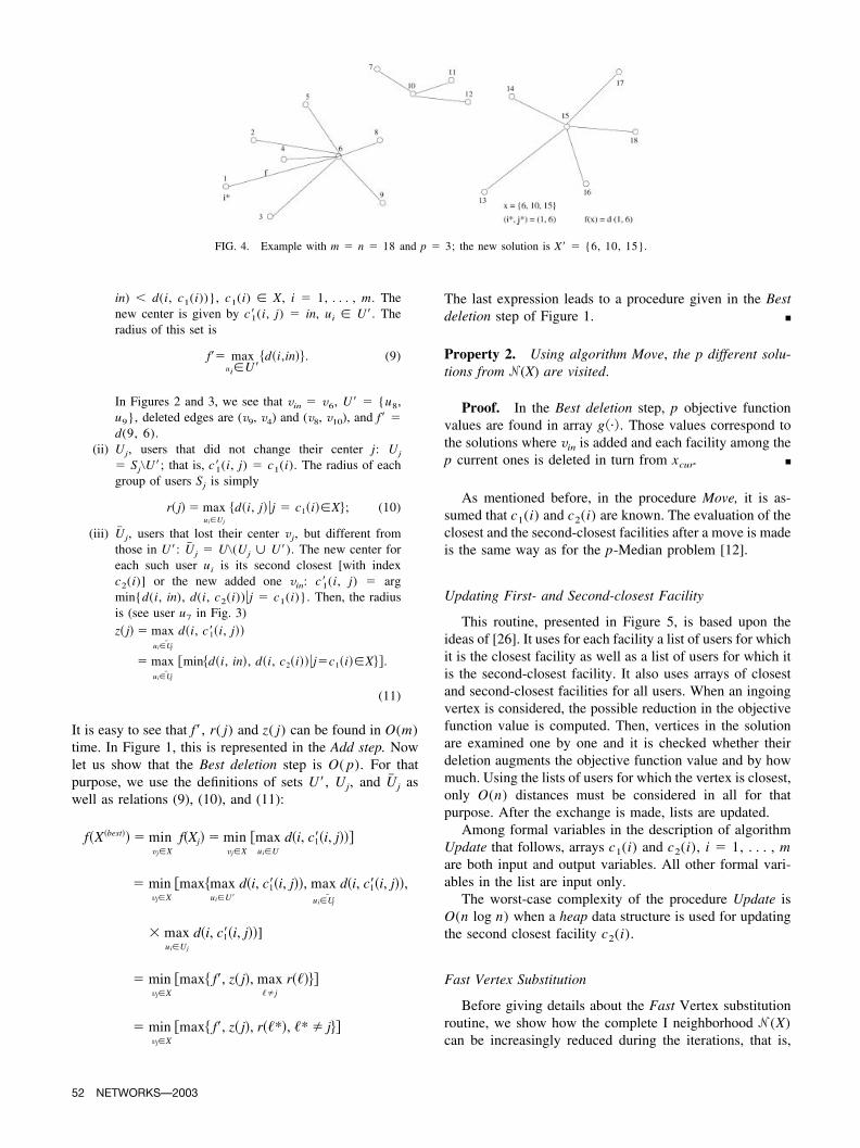
in) � d(i, c1(i))}, c1(i) � X, i � 1, . . . , m. Thenew center is given by c�1(i, j) � in, ui � U�. Theradius of this set is

f�� maxui�U�

�d�i,in��. (9)

In Figures 2 and 3, we see that vin � v6, U� � {u8,u9}, deleted edges are (v9, v4) and (v8, v10), and f� �d(9, 6).

(ii) Uj, users that did not change their center j: Uj

� Sj�U�; that is, c�1(i, j) � c1(i). The radius of eachgroup of users Sj is simply

r� j� � maxui�Uj

�d�i, j��j � c1�i��X�; (10)

(iii) U� j, users that lost their center vj, but different fromthose in U�: U� j � U�(Uj � U�). The new center foreach such user ui is its second closest [with indexc2(i)] or the new added one vin: c�1(i, j) � argmin{d(i, in), d(i, c2(i))�j � c1(i)}. Then, the radiusis (see user u7 in Fig. 3)z� j� � max

ui�U� j

d�i, c�1�i, j��

� maxui�U� j

min�d�i, in�, d�i, c2�i���j�c1�i��X�.

(11)

It is easy to see that f�, r( j) and z( j) can be found in O(m)time. In Figure 1, this is represented in the Add step. Nowlet us show that the Best deletion step is O( p). For thatpurpose, we use the definitions of sets U�, Uj, and U� j aswell as relations (9), (10), and (11):

f�X�best�� � minvj�X

f�Xj� � minvj�X

maxui�U

d�i, c�1�i, j��

� minvj�X

max�maxui�U�

d�i, c�1�i, j��, maxui�U� j

d�i, c�1�i, j��,

� maxui�Uj

d�i, c�1�i, j��]

� minvj�X

max� f�, z� j�, max��j

r����

� minvj�X

max� f�, z� j�, r��*�, �* � j�

The last expression leads to a procedure given in the Bestdeletion step of Figure 1. ■

Property 2. Using algorithm Move, the p different solu-tions from �(X) are visited.

Proof. In the Best deletion step, p objective functionvalues are found in array g�. Those values correspond tothe solutions where vin is added and each facility among thep current ones is deleted in turn from xcur. ■

As mentioned before, in the procedure Move, it is as-sumed that c1(i) and c2(i) are known. The evaluation of theclosest and the second-closest facilities after a move is madeis the same way as for the p-Median problem [12].

Updating First- and Second-closest Facility

This routine, presented in Figure 5, is based upon theideas of [26]. It uses for each facility a list of users for whichit is the closest facility as well as a list of users for which itis the second-closest facility. It also uses arrays of closestand second-closest facilities for all users. When an ingoingvertex is considered, the possible reduction in the objectivefunction value is computed. Then, vertices in the solutionare examined one by one and it is checked whether theirdeletion augments the objective function value and by howmuch. Using the lists of users for which the vertex is closest,only O(n) distances must be considered in all for thatpurpose. After the exchange is made, lists are updated.

Among formal variables in the description of algorithmUpdate that follows, arrays c1(i) and c2(i), i � 1, . . . , mare both input and output variables. All other formal vari-ables in the list are input only.

The worst-case complexity of the procedure Update isO(n log n) when a heap data structure is used for updatingthe second closest facility c2(i).

Fast Vertex Substitution

Before giving details about the Fast Vertex substitutionroutine, we show how the complete I neighborhood �(X)can be increasingly reduced during the iterations, that is,

FIG. 4. Example with m � n � 18 and p � 3; the new solution is X� � {6, 10, 15}.

52 NETWORKS—2003

how this local search can be accelerated. However, thisacceleration reduces only the constant in the heuristic’scomplexity, but not its worst-case behavior.

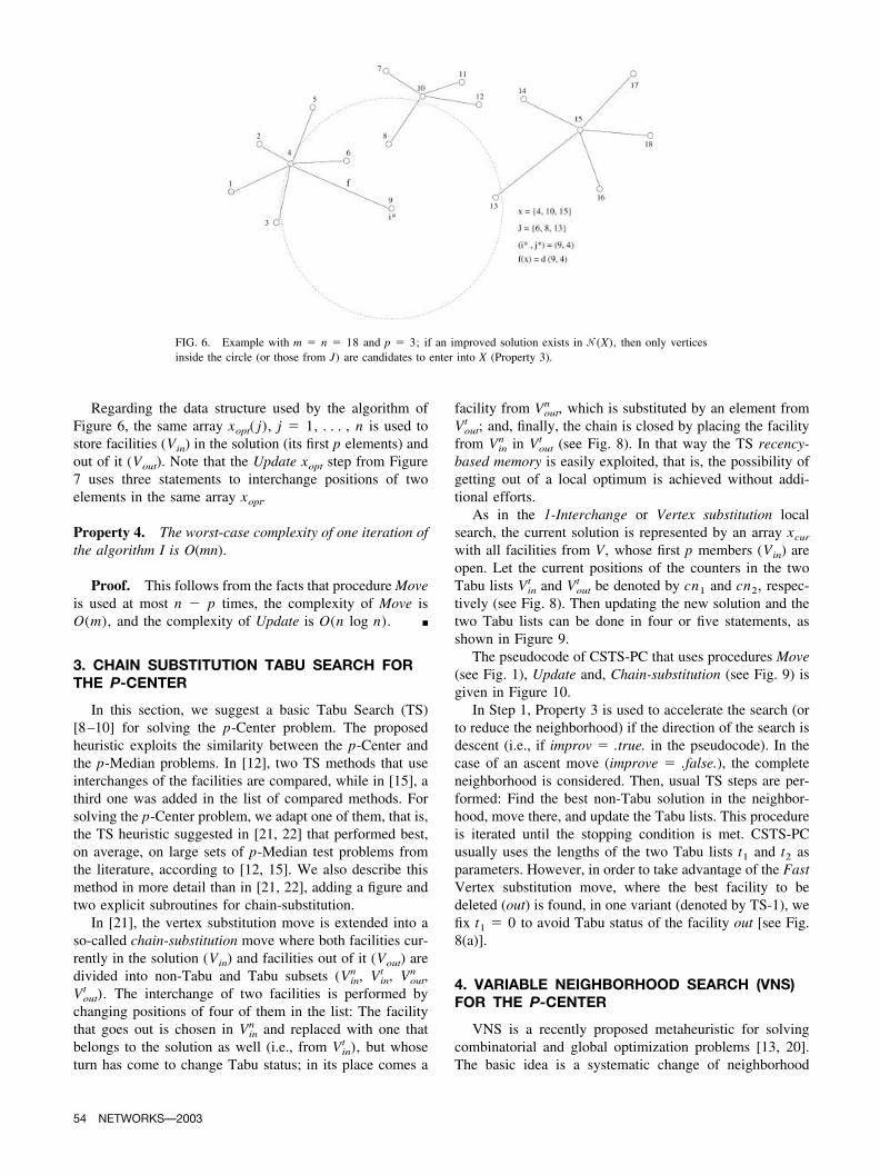
Let the current value f(X) be determined by the distancebetween a user with index i* and its closest facility j* �c1(i*) [ f � d(ui*, vj*)]. We call critical the user ui* whodetermines the objective function value. It is easy to see thatthere will be no improvement of f in �(X) if the facility tobe added is farther from the critical user (with index i*)than facility j* � c1(i*) (see Fig. 6). In other words, wehave the following:

Property 3. If there is a better solution in the vertexsubstitution neighborhood �(X) of the current solution X,then the new facility vj� must be closer to the critical user ui*

than his or her previous center vj*.

Proof. Let i� and j� � c1(i�) be the new critical vertexand the new facility, respectively ( j� � X). The result

follows easily by contradiction. Assume that d(ui*, vj�)� d(ui*, vj*). Then, the critical user ui* cannot find afacility closer than vj*. Thus, the objective function valuecannot be improved, which is a contradiction. ■

This simple fact allows us to reduce the size of thecomplete p � (n � p) neighborhood of X to p � �J(i*)�,where

J�i*� � � j�d�i*, j� � f�X��. (12)

Moreover, this size decreases with subsequent iterationsand, thus, the speed of convergence to a local minimumincreases on average. Therefore, the vertex substitution lo-cal search is more efficient in solving the p-Center problemthan in solving the p-Median problem. Its pseudocode isgiven in Figure 7. It uses the two procedures Move andUpdate.

FIG. 5. Pseudocode for procedure update within fast 1-interchange method.

NETWORKS—2003 53

Regarding the data structure used by the algorithm ofFigure 6, the same array xopt( j), j � 1, . . . , n is used tostore facilities (Vin) in the solution (its first p elements) andout of it (Vout). Note that the Update xopt step from Figure7 uses three statements to interchange positions of twoelements in the same array xopt.

Property 4. The worst-case complexity of one iteration ofthe algorithm I is O(mn).

Proof. This follows from the facts that procedure Moveis used at most n � p times, the complexity of Move isO(m), and the complexity of Update is O(n log n). ■

3. CHAIN SUBSTITUTION TABU SEARCH FORTHE P-CENTER

In this section, we suggest a basic Tabu Search (TS)[8–10] for solving the p-Center problem. The proposedheuristic exploits the similarity between the p-Center andthe p-Median problems. In [12], two TS methods that useinterchanges of the facilities are compared, while in [15], athird one was added in the list of compared methods. Forsolving the p-Center problem, we adapt one of them, that is,the TS heuristic suggested in [21, 22] that performed best,on average, on large sets of p-Median test problems fromthe literature, according to [12, 15]. We also describe thismethod in more detail than in [21, 22], adding a figure andtwo explicit subroutines for chain-substitution.

In [21], the vertex substitution move is extended into aso-called chain-substitution move where both facilities cur-rently in the solution (Vin) and facilities out of it (Vout) aredivided into non-Tabu and Tabu subsets (Vin

n , Vint , Vout

n ,Vout

t ). The interchange of two facilities is performed bychanging positions of four of them in the list: The facilitythat goes out is chosen in Vin

n and replaced with one thatbelongs to the solution as well (i.e., from Vin

t ), but whoseturn has come to change Tabu status; in its place comes a

facility from Voutn , which is substituted by an element from

Voutt ; and, finally, the chain is closed by placing the facility

from Vinn in Vout

t (see Fig. 8). In that way the TS recency-based memory is easily exploited, that is, the possibility ofgetting out of a local optimum is achieved without addi-tional efforts.

As in the 1-Interchange or Vertex substitution localsearch, the current solution is represented by an array xcur

with all facilities from V, whose first p members (Vin) areopen. Let the current positions of the counters in the twoTabu lists Vin

t and Voutt be denoted by cn1 and cn2, respec-

tively (see Fig. 8). Then updating the new solution and thetwo Tabu lists can be done in four or five statements, asshown in Figure 9.

The pseudocode of CSTS-PC that uses procedures Move(see Fig. 1), Update and, Chain-substitution (see Fig. 9) isgiven in Figure 10.

In Step 1, Property 3 is used to accelerate the search (orto reduce the neighborhood) if the direction of the search isdescent (i.e., if improv � .true. in the pseudocode). In thecase of an ascent move (improve � .false.), the completeneighborhood is considered. Then, usual TS steps are per-formed: Find the best non-Tabu solution in the neighbor-hood, move there, and update the Tabu lists. This procedureis iterated until the stopping condition is met. CSTS-PCusually uses the lengths of the two Tabu lists t1 and t2 asparameters. However, in order to take advantage of the FastVertex substitution move, where the best facility to bedeleted (out) is found, in one variant (denoted by TS-1), wefix t1 � 0 to avoid Tabu status of the facility out [see Fig.8(a)].

4. VARIABLE NEIGHBORHOOD SEARCH (VNS)FOR THE P-CENTER

VNS is a recently proposed metaheuristic for solvingcombinatorial and global optimization problems [13, 20].The basic idea is a systematic change of neighborhood

FIG. 6. Example with m � n � 18 and p � 3; if an improved solution exists in �(X), then only verticesinside the circle (or those from J) are candidates to enter into X (Property 3).

54 NETWORKS—2003

structures within a local search algorithm. The algorithmremains centered around the same solution until anothersolution better than the incumbent is found and then jumpsthere. So, it is not a trajectory-following method such asSimulated Annealing or TS. By exploiting the empiricalproperty of closeness of local minima that holds for mostcombinatorial problems, the basic VNS heuristic securestwo important advantages: (i) by staying in the neighbor-hood of the incumbent the search is done in an attractivearea of the solution space which is not, moreover, perturbedby forbidden moves; and (ii) as some of the solution at-tributes are already in their optimal values, local search usesseveral times fewer iterations than if initialized with arandom solution, so, it may visit several high-quality localoptima in the same CPU time one descent from a randomsolution takes to visit only one.

Let us denote by � � {X�X � set of p (out of m)locations of facilities} a solution space of the problem. Wesay that the distance between two solutions X1 and X2 (X1,X2 � �) is equal to k, if and only if they differ in k

FIG. 7. Description of the fast vertex substitution or the 1-interchange (I) descent method.

FIG. 8. Chain-substitution management: (a) TS-1: interchanges with useof one Tabu list (Vin

t � A); (b) TS-2: use of two Tabu lists.

NETWORKS—2003 55

FIG. 9. Chain vertex substitution with one and two Tabu lists.

FIG. 10. Pseudocode for CSTS-PC method.

56 NETWORKS—2003

locations. Since � is a set of sets, a (symmetric) distancefunction can be defined as

�X1, X2� � �X1�X2� � �X2�X1�, � X1, X2 � X. (13)

It can easily be checked that is a metric function in �; thus,� is a metric space. The neighborhood structures that we useare induced by the metric , that is, k locations of facilities(k � p) from the current solution are replaced by k others.We denote by �k, k � 1, . . . , kmax (kmax � p) the set ofsuch neighborhood structures and by �k(X) the set ofsolutions forming neighborhood �k of a current solution X.More formally,

X� � �k�X� N �X�, X� � k. (14)

Another property of the p-Center problem that we mustkeep in mind in developing a VNS heuristic is the existenceof many solutions with the same objective function value.This is especially the case for local minima. Indeed, bykeeping the same critical user and its center (i.e., the sameobjective value), one can sometimes find many ways toselect another p � 1 centers other than those in the currentsolution. For example, assume that n � m � 300 users aredivided in p � 3 very distant groups A, B, and C, eachhaving 100 users in a current solution; assume further thatthe critical user is in group A and that the value f is largerthan the diameters of both groups B and C. Then, there are100 � 100 � 10,000 solutions with the same value f.

The basic VNS may have difficulties escaping from thefirst found local optima among many with the same objec-tive function value. Note that TS has no such difficulty sinceit keeps moving whether the new solution is better, equal, orworse. To overcome this in VNS, we always move to asolution of equal value, as in TS. There are other ways toescape from “plateau” solutions that we tried also: (i) to useadditional criteria such as the p-Median and the p-Center-sum [11] values. The latter criterion gave better results thandid the former; however, it was not better, on average, thana simple move to a solution with equal value; and (ii) tomake a move with some probability (a parameter). Al-though we found that this parameter is closely related to p(a smaller probability is better for small p), the differencesin solution value were again not significant. We concludethat there is no need to introduce additional criteria orparameters in the basic VNS version.

Pseudocode for our VNS algorithm for the p-Centerproblem (VNS-PC) is given in Figure 11. It uses proceduresMove and Update (from Section 2).

In Step 2a, the incumbent solution X is perturbed in sucha way that (X, X�) � k. As in I local search and in TS, weuse here Property 3 to reduce the size of �k(X). Then, X� isused as the initial solution for fast vertex substitution in Step2b. If an equal or better solution than X is obtained, wemove there and start again with small perturbations of thisnew best solution (i.e., k 4 1). Otherwise, we increase the

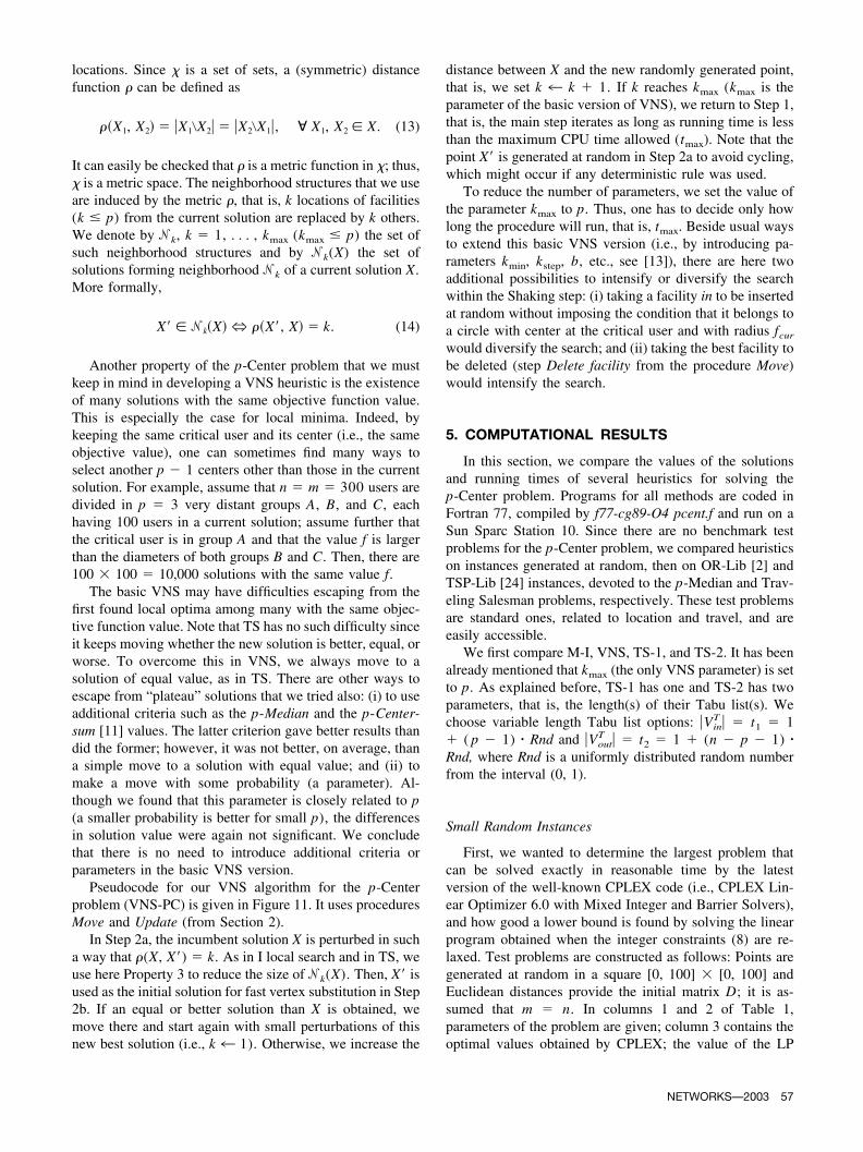
distance between X and the new randomly generated point,that is, we set k 4 k 1. If k reaches kmax (kmax is theparameter of the basic version of VNS), we return to Step 1,that is, the main step iterates as long as running time is lessthan the maximum CPU time allowed (tmax). Note that thepoint X� is generated at random in Step 2a to avoid cycling,which might occur if any deterministic rule was used.

To reduce the number of parameters, we set the value ofthe parameter kmax to p. Thus, one has to decide only howlong the procedure will run, that is, tmax. Beside usual waysto extend this basic VNS version (i.e., by introducing pa-rameters kmin, kstep, b, etc., see [13]), there are here twoadditional possibilities to intensify or diversify the searchwithin the Shaking step: (i) taking a facility in to be insertedat random without imposing the condition that it belongs toa circle with center at the critical user and with radius fcur

would diversify the search; and (ii) taking the best facility tobe deleted (step Delete facility from the procedure Move)would intensify the search.

5. COMPUTATIONAL RESULTS

In this section, we compare the values of the solutionsand running times of several heuristics for solving thep-Center problem. Programs for all methods are coded inFortran 77, compiled by f77-cg89-O4 pcent.f and run on aSun Sparc Station 10. Since there are no benchmark testproblems for the p-Center problem, we compared heuristicson instances generated at random, then on OR-Lib [2] andTSP-Lib [24] instances, devoted to the p-Median and Trav-eling Salesman problems, respectively. These test problemsare standard ones, related to location and travel, and areeasily accessible.

We first compare M-I, VNS, TS-1, and TS-2. It has beenalready mentioned that kmax (the only VNS parameter) is setto p. As explained before, TS-1 has one and TS-2 has twoparameters, that is, the length(s) of their Tabu list(s). Wechoose variable length Tabu list options: �Vin

T � � t1 � 1 ( p � 1) � Rnd and �Vout

T � � t2 � 1 (n � p � 1) �Rnd, where Rnd is a uniformly distributed random numberfrom the interval (0, 1).

Small Random Instances

First, we wanted to determine the largest problem thatcan be solved exactly in reasonable time by the latestversion of the well-known CPLEX code (i.e., CPLEX Lin-ear Optimizer 6.0 with Mixed Integer and Barrier Solvers),and how good a lower bound is found by solving the linearprogram obtained when the integer constraints (8) are re-laxed. Test problems are constructed as follows: Points aregenerated at random in a square [0, 100] � [0, 100] andEuclidean distances provide the initial matrix D; it is as-sumed that m � n. In columns 1 and 2 of Table 1,parameters of the problem are given; column 3 contains theoptimal values obtained by CPLEX; the value of the LP

NETWORKS—2003 57

solution and % gap are given in columns 4 and 5, respec-tively, where % gap is calculated as

fex flp

fex� 100%. (15)

The next three columns report CPLEX outputs: Running

time, number of iterations, and number of search tree nodes.The best values obtained with the three metaheuristics pro-posed in this paper (i.e., M-I, VNS, and TS) and B-S [16]are given in columns 9–12.

It appears that (i) one has to wait almost 8 hours to getthe exact solution ( fex) when n � m � 40 and p � 10; (ii)all three metaheuristics proposed in this paper (i.e., M-I,

FIG. 11. Pseudocode for VNS-PC method.

58 NETWORKS—2003

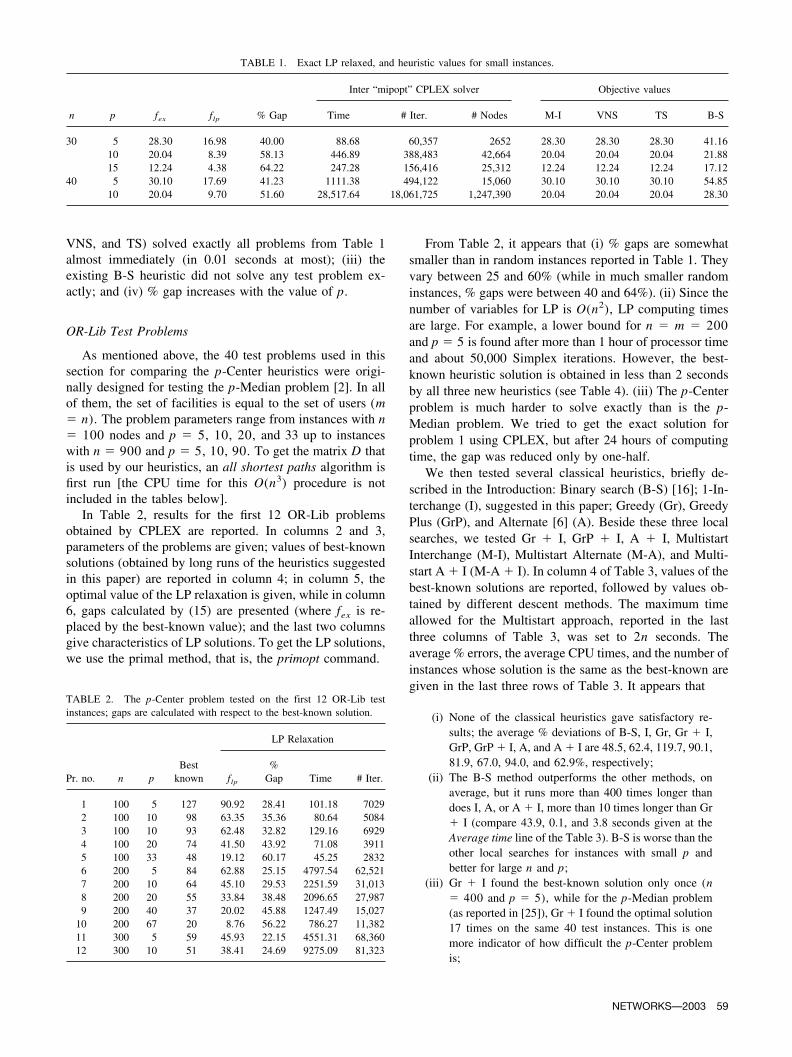
VNS, and TS) solved exactly all problems from Table 1almost immediately (in 0.01 seconds at most); (iii) theexisting B-S heuristic did not solve any test problem ex-actly; and (iv) % gap increases with the value of p.

OR-Lib Test Problems

As mentioned above, the 40 test problems used in thissection for comparing the p-Center heuristics were origi-nally designed for testing the p-Median problem [2]. In allof them, the set of facilities is equal to the set of users (m� n). The problem parameters range from instances with n� 100 nodes and p � 5, 10, 20, and 33 up to instanceswith n � 900 and p � 5, 10, 90. To get the matrix D thatis used by our heuristics, an all shortest paths algorithm isfirst run [the CPU time for this O(n3) procedure is notincluded in the tables below].

In Table 2, results for the first 12 OR-Lib problemsobtained by CPLEX are reported. In columns 2 and 3,parameters of the problems are given; values of best-knownsolutions (obtained by long runs of the heuristics suggestedin this paper) are reported in column 4; in column 5, theoptimal value of the LP relaxation is given, while in column6, gaps calculated by (15) are presented (where fex is re-placed by the best-known value); and the last two columnsgive characteristics of LP solutions. To get the LP solutions,we use the primal method, that is, the primopt command.

From Table 2, it appears that (i) % gaps are somewhatsmaller than in random instances reported in Table 1. Theyvary between 25 and 60% (while in much smaller randominstances, % gaps were between 40 and 64%). (ii) Since thenumber of variables for LP is O(n2), LP computing timesare large. For example, a lower bound for n � m � 200and p � 5 is found after more than 1 hour of processor timeand about 50,000 Simplex iterations. However, the best-known heuristic solution is obtained in less than 2 secondsby all three new heuristics (see Table 4). (iii) The p-Centerproblem is much harder to solve exactly than is the p-Median problem. We tried to get the exact solution forproblem 1 using CPLEX, but after 24 hours of computingtime, the gap was reduced only by one-half.

We then tested several classical heuristics, briefly de-scribed in the Introduction: Binary search (B-S) [16]; 1-In-terchange (I), suggested in this paper; Greedy (Gr), GreedyPlus (GrP), and Alternate [6] (A). Beside these three localsearches, we tested Gr I, GrP I, A I, MultistartInterchange (M-I), Multistart Alternate (M-A), and Multi-start A I (M-A I). In column 4 of Table 3, values of thebest-known solutions are reported, followed by values ob-tained by different descent methods. The maximum timeallowed for the Multistart approach, reported in the lastthree columns of Table 3, was set to 2n seconds. Theaverage % errors, the average CPU times, and the number ofinstances whose solution is the same as the best-known aregiven in the last three rows of Table 3. It appears that

(i) None of the classical heuristics gave satisfactory re-sults; the average % deviations of B-S, I, Gr, Gr I,GrP, GrP I, A, and A I are 48.5, 62.4, 119.7, 90.1,81.9, 67.0, 94.0, and 62.9%, respectively;

(ii) The B-S method outperforms the other methods, onaverage, but it runs more than 400 times longer thandoes I, A, or A I, more than 10 times longer than Gr I (compare 43.9, 0.1, and 3.8 seconds given at theAverage time line of the Table 3). B-S is worse than theother local searches for instances with small p andbetter for large n and p;

(iii) Gr I found the best-known solution only once (n� 400 and p � 5), while for the p-Median problem(as reported in [25]), Gr I found the optimal solution17 times on the same 40 test instances. This is onemore indicator of how difficult the p-Center problemis;

TABLE 1. Exact LP relaxed, and heuristic values for small instances.

n p fex flp % Gap

Inter “mipopt” CPLEX solver Objective values

Time # Iter. # Nodes M-I VNS TS B-S

30 5 28.30 16.98 40.00 88.68 60,357 2652 28.30 28.30 28.30 41.1610 20.04 8.39 58.13 446.89 388,483 42,664 20.04 20.04 20.04 21.8815 12.24 4.38 64.22 247.28 156,416 25,312 12.24 12.24 12.24 17.12

40 5 30.10 17.69 41.23 1111.38 494,122 15,060 30.10 30.10 30.10 54.8510 20.04 9.70 51.60 28,517.64 18,061,725 1,247,390 20.04 20.04 20.04 28.30

TABLE 2. The p-Center problem tested on the first 12 OR-Lib testinstances; gaps are calculated with respect to the best-known solution.

Pr. no. n pBest

known

LP Relaxation

flp

%Gap Time # Iter.

1 100 5 127 90.92 28.41 101.18 70292 100 10 98 63.35 35.36 80.64 50843 100 10 93 62.48 32.82 129.16 69294 100 20 74 41.50 43.92 71.08 39115 100 33 48 19.12 60.17 45.25 28326 200 5 84 62.88 25.15 4797.54 62,5217 200 10 64 45.10 29.53 2251.59 31,0138 200 20 55 33.84 38.48 2096.65 27,9879 200 40 37 20.02 45.88 1247.49 15,027

10 200 67 20 8.76 56.22 786.27 11,38211 300 5 59 45.93 22.15 4551.31 68,36012 300 10 51 38.41 24.69 9275.09 81,323

NETWORKS—2003 59

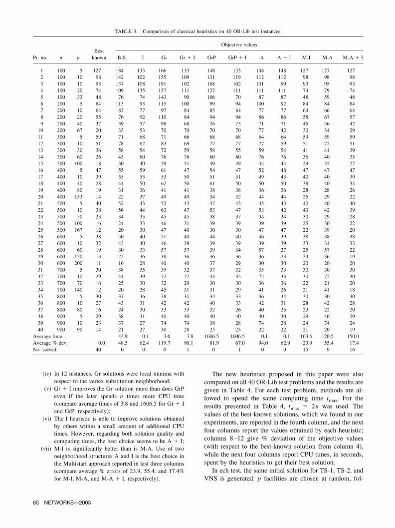
(iv) In 12 instances, Gr solutions were local minima withrespect to the vertex substitution neighborhood;

(v) Gr I improves the Gr solution more than does GrPeven if the later spends n times more CPU time(compare average times of 3.8 and 1606.5 for Gr Iand GrP, respectively);

(vi) The I heuristic is able to improve solutions obtainedby others within a small amount of additional CPUtimes. However, regarding both solution quality andcomputing times, the best choice seems to be A I;

(vii) M-I is significantly better than is M-A. Use of twoneighborhood structures A and I is the best choice inthe Multistart approach reported in last three columns(compare average % errors of 23.9, 55.4, and 17.4%for M-I, M-A, and M-A I, respectively).

The new heuristics proposed in this paper were alsocompared on all 40 OR-Lib test problems and the results aregiven in Table 4. For each test problem, methods are al-lowed to spend the same computing time tmax. For theresults presented in Table 4, tmax � 2n was used. Thevalues of the best-known solutions, which we found in ourexperiments, are reported in the fourth column, and the nextfour columns report the values obtained by each heuristic;columns 8–12 give % deviation of the objective values(with respect to the best-known solution from column 4),while the next four columns report CPU times, in seconds,spent by the heuristics to get their best solution.

In ech test, the same initial solution for TS-1, TS-2, andVNS is generated: p facilities are chosen at random, fol-

TABLE 3. Comparison of classical heuristics on 40 OR-Lib test instances.

Pr. no. n pBest

known

Objective values

B-S I Gr Gr I GrP GrP I A A I M-I M-A M-A I

1 100 5 127 184 133 166 133 148 133 148 148 127 127 1272 100 10 98 142 102 155 109 131 119 112 112 98 98 983 100 10 93 137 108 191 102 168 102 131 99 93 95 934 100 20 74 109 135 157 111 127 111 111 111 74 79 745 100 33 48 76 74 143 90 106 70 87 87 48 59 486 200 5 84 113 93 115 100 99 94 100 92 84 84 847 200 10 64 87 77 97 84 85 84 77 77 64 66 648 200 20 55 76 92 110 84 94 94 86 86 58 67 579 200 40 37 59 57 98 68 76 73 71 71 46 56 42

10 200 67 20 33 53 70 70 70 70 77 42 30 34 2911 300 5 59 71 68 71 66 68 68 64 64 59 59 5912 300 10 51 78 62 83 69 77 77 77 59 51 72 5113 300 30 36 58 54 72 59 58 55 59 54 41 41 3914 300 60 26 43 60 76 76 60 60 76 76 36 40 3515 300 100 18 30 40 59 51 49 49 44 44 29 35 2716 400 5 47 55 59 61 47 54 47 52 48 47 47 4717 400 10 39 55 53 53 50 51 51 49 43 40 40 3918 400 40 28 44 50 62 50 61 50 50 50 38 40 3419 400 80 19 31 36 41 41 38 38 36 36 28 28 2620 400 133 14 22 37 49 49 34 32 44 44 26 29 2221 500 5 40 52 43 52 43 47 43 45 43 40 40 4022 500 10 38 56 44 63 47 53 47 53 42 40 42 3923 500 50 23 34 35 45 45 38 37 34 34 30 29 2824 500 100 16 24 33 46 31 39 39 39 39 25 30 2225 500 167 12 20 30 47 40 30 30 47 47 22 39 2026 600 5 38 50 40 51 40 44 40 46 39 38 38 3827 600 10 32 43 40 46 39 39 39 39 39 33 34 3328 600 60 19 30 33 57 57 39 34 57 27 25 57 2229 600 120 13 22 36 38 36 36 36 36 23 23 36 1930 600 200 11 16 28 40 40 37 29 30 30 20 20 2031 700 5 30 38 35 39 32 37 32 35 33 30 30 3032 700 10 29 44 39 72 72 44 35 72 33 30 72 3033 700 70 16 25 30 32 29 30 30 36 36 22 21 2034 700 140 12 20 28 45 31 31 29 41 26 21 41 1835 800 5 30 37 36 38 31 34 33 36 34 30 30 3036 800 10 27 43 31 42 42 40 33 42 31 28 42 2837 800 80 16 24 30 33 33 32 26 40 25 23 22 2038 900 5 29 38 31 40 40 40 40 40 30 29 40 2939 900 10 23 37 27 74 74 38 28 74 28 24 74 2440 900 90 14 21 27 30 28 25 25 22 22 21 20 19

Average time 43.9 0.1 3.6 3.8 1606.5 1606.5 0.1 0.1 163.6 120.5 150.0Average % dev. 0.0 48.5 62.4 119.7 90.1 81.9 67.0 94.0 62.9 23.9 55.4 17.4No. solved 40 0 0 0 1 0 1 0 0 15 9 16

60 NETWORKS—2003

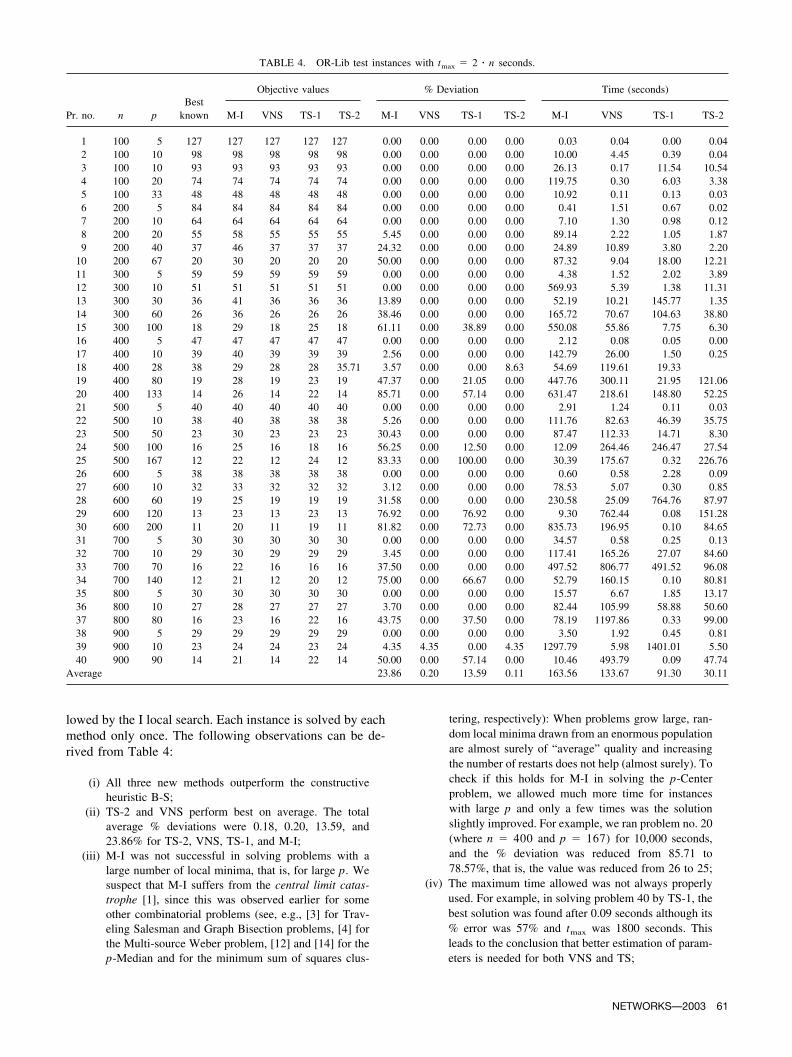
lowed by the I local search. Each instance is solved by eachmethod only once. The following observations can be de-rived from Table 4:

(i) All three new methods outperform the constructiveheuristic B-S;

(ii) TS-2 and VNS perform best on average. The totalaverage % deviations were 0.18, 0.20, 13.59, and23.86% for TS-2, VNS, TS-1, and M-I;

(iii) M-I was not successful in solving problems with alarge number of local minima, that is, for large p. Wesuspect that M-I suffers from the central limit catas-trophe [1], since this was observed earlier for someother combinatorial problems (see, e.g., [3] for Trav-eling Salesman and Graph Bisection problems, [4] forthe Multi-source Weber problem, [12] and [14] for thep-Median and for the minimum sum of squares clus-

tering, respectively): When problems grow large, ran-dom local minima drawn from an enormous populationare almost surely of “average” quality and increasingthe number of restarts does not help (almost surely). Tocheck if this holds for M-I in solving the p-Centerproblem, we allowed much more time for instanceswith large p and only a few times was the solutionslightly improved. For example, we ran problem no. 20(where n � 400 and p � 167) for 10,000 seconds,and the % deviation was reduced from 85.71 to78.57%, that is, the value was reduced from 26 to 25;

(iv) The maximum time allowed was not always properlyused. For example, in solving problem 40 by TS-1, thebest solution was found after 0.09 seconds although its% error was 57% and tmax was 1800 seconds. Thisleads to the conclusion that better estimation of param-eters is needed for both VNS and TS;

TABLE 4. OR-Lib test instances with tmax � 2 � n seconds.

Pr. no. n pBest

known

Objective values % Deviation Time (seconds)

M-I VNS TS-1 TS-2 M-I VNS TS-1 TS-2 M-I VNS TS-1 TS-2

1 100 5 127 127 127 127 127 0.00 0.00 0.00 0.00 0.03 0.04 0.00 0.042 100 10 98 98 98 98 98 0.00 0.00 0.00 0.00 10.00 4.45 0.39 0.043 100 10 93 93 93 93 93 0.00 0.00 0.00 0.00 26.13 0.17 11.54 10.544 100 20 74 74 74 74 74 0.00 0.00 0.00 0.00 119.75 0.30 6.03 3.385 100 33 48 48 48 48 48 0.00 0.00 0.00 0.00 10.92 0.11 0.13 0.036 200 5 84 84 84 84 84 0.00 0.00 0.00 0.00 0.41 1.51 0.67 0.027 200 10 64 64 64 64 64 0.00 0.00 0.00 0.00 7.10 1.30 0.98 0.128 200 20 55 58 55 55 55 5.45 0.00 0.00 0.00 89.14 2.22 1.05 1.879 200 40 37 46 37 37 37 24.32 0.00 0.00 0.00 24.89 10.89 3.80 2.20

10 200 67 20 30 20 20 20 50.00 0.00 0.00 0.00 87.32 9.04 18.00 12.2111 300 5 59 59 59 59 59 0.00 0.00 0.00 0.00 4.38 1.52 2.02 3.8912 300 10 51 51 51 51 51 0.00 0.00 0.00 0.00 569.93 5.39 1.38 11.3113 300 30 36 41 36 36 36 13.89 0.00 0.00 0.00 52.19 10.21 145.77 1.3514 300 60 26 36 26 26 26 38.46 0.00 0.00 0.00 165.72 70.67 104.63 38.8015 300 100 18 29 18 25 18 61.11 0.00 38.89 0.00 550.08 55.86 7.75 6.3016 400 5 47 47 47 47 47 0.00 0.00 0.00 0.00 2.12 0.08 0.05 0.0017 400 10 39 40 39 39 39 2.56 0.00 0.00 0.00 142.79 26.00 1.50 0.2518 400 28 38 29 28 28 35.71 3.57 0.00 0.00 8.63 54.69 119.61 19.3319 400 80 19 28 19 23 19 47.37 0.00 21.05 0.00 447.76 300.11 21.95 121.0620 400 133 14 26 14 22 14 85.71 0.00 57.14 0.00 631.47 218.61 148.80 52.2521 500 5 40 40 40 40 40 0.00 0.00 0.00 0.00 2.91 1.24 0.11 0.0322 500 10 38 40 38 38 38 5.26 0.00 0.00 0.00 111.76 82.63 46.39 35.7523 500 50 23 30 23 23 23 30.43 0.00 0.00 0.00 87.47 112.33 14.71 8.3024 500 100 16 25 16 18 16 56.25 0.00 12.50 0.00 12.09 264.46 246.47 27.5425 500 167 12 22 12 24 12 83.33 0.00 100.00 0.00 30.39 175.67 0.32 226.7626 600 5 38 38 38 38 38 0.00 0.00 0.00 0.00 0.60 0.58 2.28 0.0927 600 10 32 33 32 32 32 3.12 0.00 0.00 0.00 78.53 5.07 0.30 0.8528 600 60 19 25 19 19 19 31.58 0.00 0.00 0.00 230.58 25.09 764.76 87.9729 600 120 13 23 13 23 13 76.92 0.00 76.92 0.00 9.30 762.44 0.08 151.2830 600 200 11 20 11 19 11 81.82 0.00 72.73 0.00 835.73 196.95 0.10 84.6531 700 5 30 30 30 30 30 0.00 0.00 0.00 0.00 34.57 0.58 0.25 0.1332 700 10 29 30 29 29 29 3.45 0.00 0.00 0.00 117.41 165.26 27.07 84.6033 700 70 16 22 16 16 16 37.50 0.00 0.00 0.00 497.52 806.77 491.52 96.0834 700 140 12 21 12 20 12 75.00 0.00 66.67 0.00 52.79 160.15 0.10 80.8135 800 5 30 30 30 30 30 0.00 0.00 0.00 0.00 15.57 6.67 1.85 13.1736 800 10 27 28 27 27 27 3.70 0.00 0.00 0.00 82.44 105.99 58.88 50.6037 800 80 16 23 16 22 16 43.75 0.00 37.50 0.00 78.19 1197.86 0.33 99.0038 900 5 29 29 29 29 29 0.00 0.00 0.00 0.00 3.50 1.92 0.45 0.8139 900 10 23 24 24 23 24 4.35 4.35 0.00 4.35 1297.79 5.98 1401.01 5.5040 900 90 14 21 14 22 14 50.00 0.00 57.14 0.00 10.46 493.79 0.09 47.74

Average 23.86 0.20 13.59 0.11 163.56 133.67 91.30 30.11

NETWORKS—2003 61

(v) TS-1 was developed in order to exploit Observation 1made above in full. In other words, we wanted toprevent situations where some good move had beenmade Tabu. However, although in the first stage of thesearch it looks very efficient, after some time, TS-1becomes over intensified and cannot escape easilyfrom deep local optima.

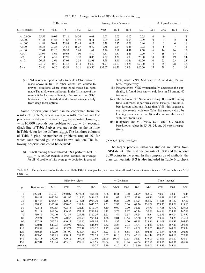
Some observations above can be confirmed from theresults of Table 5, where average results over all 40 testproblems for different values of tmax are reported: From tmax

� n/10,000 seconds per problem to tmax � 2n seconds.(Each line of Table 5 gives average results, as the last linein Table 4, but for the different tmax). The last three columnsof Table 5 give the number of problems (out of 40) forwhich each method got the best-known solution. The fol-lowing observations could be derived:

(i) If small running time is allowed, TS-1 performs best. Iftmax � n/10,000 (which is 0.05 seconds on averagefor all 40 problems), its average % deviation is around

37%, while VNS, M-I, and TS-2 yield 49, 55, and66%, respectively;

(ii) Parameterless VNS systematically decreases the gap;finally, it found best-known solutions in 38 among 40instances;

(iii) The behavior of TS-2 is interesting: If a small runningtime is allowed, it performs worst. Finally, it found 39best-known solutions, faster than VNS; this suggest tostart the search with one Tabu list strategy (i.e., bykeeping parameter t1 � 0) and continue the searchwith two Tabu lists;

(iv) It appears that M-I, VNS, TS-1, and TS-2 reachedbest-known values in 15, 38, 31, and 39 cases, respec-tively.

TSP-Lib Test Problem

The larger problem instances studied are taken fromTSP-Lib [24]. The first one consists of 1060 and the second3038 points in the plane. In the comparison of methods, theclassical heuristic B-S is also included in Table 6 to check

TABLE 5. Average results for 40 OR-Lib test instances for tmax.

tmax (seconds)

% Deviation Average times (seconds) # of problems solved

M-I VNS TS-1 TS-2 M-I VNS TS-1 TS-2 tmax M-I VNS TS-1 TS-2

n/10,000 55.55 49.05 37.11 66.36 0.08 0.07 0.03 0.02 0.05 0 0 1 2n/5000 51.44 44.22 31.67 57.93 0.11 0.09 0.05 0.04 0.09 0 1 2 4n/1000 41.84 30.44 25.98 22.43 0.22 0.28 0.17 0.28 0.46 2 3 6 11n/500 36.34 23.26 24.51 16.27 0.49 0.58 0.24 0.46 0.92 2 6 7 12n/100 32.41 12.16 20.57 7.69 1.67 2.26 0.88 4.41 4.60 6 14 16 15n/50 28.94 8.61 19.65 7.00 4.10 4.51 1.57 2.46 9.20 7 16 17 19n/20 27.14 4.55 17.98 3.37 8.05 7.52 3.21 5.83 23.00 10 20 19 24n/10 26.23 3.61 17.03 2.38 12.91 13.98 8.40 10.86 46.00 10 22 23 28n 24.19 0.70 13.37 0.18 63.42 71.97 40.63 33.24 460.00 13 35 28 382 � n 23.86 0.20 13.59 0.11 163.56 133.67 91.30 33.24 920.00 15 38 31 39

TABLE 6. The p-Center results for the n � 1060 TSP-Lib test problem; maximum time allowed for each instance is set to 500 seconds on a SUNSparc 10.

p Best known

Objective values % Deviation Time (seconds)

M-I VNS TS-1 B-S M-I VNS TS-1 B-S M-I VNS TS-1 B-S

10 2273.08 2360.71 2280.09 2273.08 3291.10 3.86 0.31 0.00 44.79 363.62 94.93 23.43 19.4820 1594.87 1650.34 1611.95 1611.92 2486.17 3.48 1.07 1.07 55.89 68.36 20.49 480.43 44.0630 1217.48 1304.87 1220.41 1217.48 1914.30 7.18 0.24 0.00 57.24 365.92 373.46 351.57 67.1940 1020.56 1105.40 1050.45 1051.74 1645.72 8.31 2.93 3.06 61.26 226.09 279.75 194.06 118.1350 922.11 950.65 922.14 922.11 1393.79 3.10 0.00 0.00 51.15 39.79 477.18 333.72 129.0660 781.17 862.56 806.52 791.08 1290.05 10.42 3.25 1.27 65.14 50.50 446.89 254.87 142.8270 710.76 790.40 721.37 727.59 1117.59 11.21 1.49 2.37 57.24 6.34 422.73 369.04 217.5780 652.21 727.59 670.53 720.93 999.84 11.56 2.81 10.54 53.30 112.95 398.84 54.29 276.6190 607.88 700.55 640.23 636.42 999.84 15.24 5.32 4.70 64.48 218.86 111.08 488.33 364.50

100 570.01 640.23 582.92 583.32 848.59 12.32 2.26 2.34 48.87 214.29 430.33 457.49 259.31110 538.84 604.44 565.72 570.18 806.52 12.17 4.99 5.82 49.68 235.05 186.60 465.06 279.34120 510.28 582.90 551.90 538.74 721.37 14.23 8.16 5.58 41.37 304.66 218.84 357.75 292.51130 499.65 582.95 500.14 538.27 728.55 16.67 0.10 7.73 45.81 441.44 473.65 469.60 375.92140 453.13 552.76 500.12 499.96 707.66 21.99 10.37 10.33 56.17 316.09 214.06 280.17 550.14150 447.01 538.84 453.16 495.02 667.55 20.54 1.38 10.74 49.34 477.56 428.16 440.86 785.94

Average 10.77 2.79 4.10 50.11 215.10 286.06 313.83 245.16

62 NETWORKS—2003

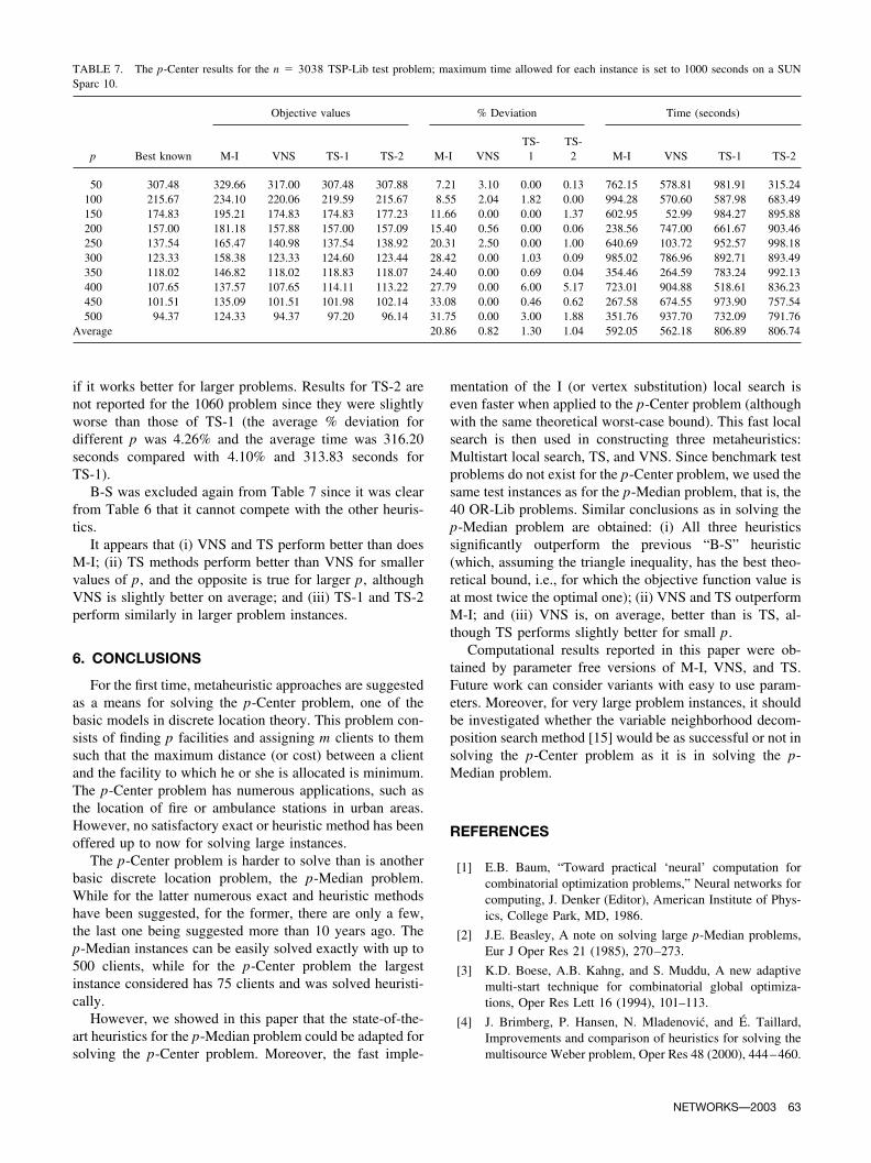
if it works better for larger problems. Results for TS-2 arenot reported for the 1060 problem since they were slightlyworse than those of TS-1 (the average % deviation fordifferent p was 4.26% and the average time was 316.20seconds compared with 4.10% and 313.83 seconds forTS-1).

B-S was excluded again from Table 7 since it was clearfrom Table 6 that it cannot compete with the other heuris-tics.

It appears that (i) VNS and TS perform better than doesM-I; (ii) TS methods perform better than VNS for smallervalues of p, and the opposite is true for larger p, althoughVNS is slightly better on average; and (iii) TS-1 and TS-2perform similarly in larger problem instances.

6. CONCLUSIONS

For the first time, metaheuristic approaches are suggestedas a means for solving the p-Center problem, one of thebasic models in discrete location theory. This problem con-sists of finding p facilities and assigning m clients to themsuch that the maximum distance (or cost) between a clientand the facility to which he or she is allocated is minimum.The p-Center problem has numerous applications, such asthe location of fire or ambulance stations in urban areas.However, no satisfactory exact or heuristic method has beenoffered up to now for solving large instances.

The p-Center problem is harder to solve than is anotherbasic discrete location problem, the p-Median problem.While for the latter numerous exact and heuristic methodshave been suggested, for the former, there are only a few,the last one being suggested more than 10 years ago. Thep-Median instances can be easily solved exactly with up to500 clients, while for the p-Center problem the largestinstance considered has 75 clients and was solved heuristi-cally.

However, we showed in this paper that the state-of-the-art heuristics for the p-Median problem could be adapted forsolving the p-Center problem. Moreover, the fast imple-

mentation of the I (or vertex substitution) local search iseven faster when applied to the p-Center problem (althoughwith the same theoretical worst-case bound). This fast localsearch is then used in constructing three metaheuristics:Multistart local search, TS, and VNS. Since benchmark testproblems do not exist for the p-Center problem, we used thesame test instances as for the p-Median problem, that is, the40 OR-Lib problems. Similar conclusions as in solving thep-Median problem are obtained: (i) All three heuristicssignificantly outperform the previous “B-S” heuristic(which, assuming the triangle inequality, has the best theo-retical bound, i.e., for which the objective function value isat most twice the optimal one); (ii) VNS and TS outperformM-I; and (iii) VNS is, on average, better than is TS, al-though TS performs slightly better for small p.

Computational results reported in this paper were ob-tained by parameter free versions of M-I, VNS, and TS.Future work can consider variants with easy to use param-eters. Moreover, for very large problem instances, it shouldbe investigated whether the variable neighborhood decom-position search method [15] would be as successful or not insolving the p-Center problem as it is in solving the p-Median problem.

REFERENCES

[1] E.B. Baum, “Toward practical ‘neural’ computation forcombinatorial optimization problems,” Neural networks forcomputing, J. Denker (Editor), American Institute of Phys-ics, College Park, MD, 1986.

[2] J.E. Beasley, A note on solving large p-Median problems,Eur J Oper Res 21 (1985), 270–273.

[3] K.D. Boese, A.B. Kahng, and S. Muddu, A new adaptivemulti-start technique for combinatorial global optimiza-tions, Oper Res Lett 16 (1994), 101–113.

[4] J. Brimberg, P. Hansen, N. Mladenovic, and E. Taillard,Improvements and comparison of heuristics for solving themultisource Weber problem, Oper Res 48 (2000), 444–460.

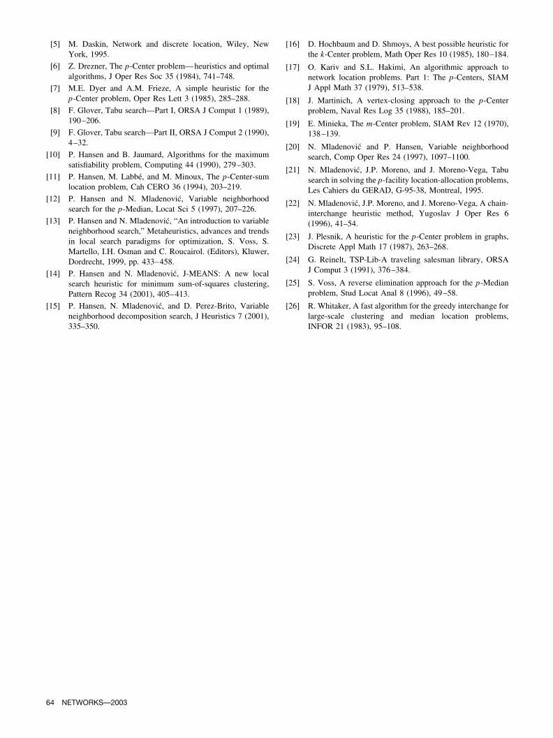
TABLE 7. The p-Center results for the n � 3038 TSP-Lib test problem; maximum time allowed for each instance is set to 1000 seconds on a SUNSparc 10.

p Best known

Objective values % Deviation Time (seconds)

M-I VNS TS-1 TS-2 M-I VNSTS-1

TS-2 M-I VNS TS-1 TS-2

50 307.48 329.66 317.00 307.48 307.88 7.21 3.10 0.00 0.13 762.15 578.81 981.91 315.24100 215.67 234.10 220.06 219.59 215.67 8.55 2.04 1.82 0.00 994.28 570.60 587.98 683.49150 174.83 195.21 174.83 174.83 177.23 11.66 0.00 0.00 1.37 602.95 52.99 984.27 895.88200 157.00 181.18 157.88 157.00 157.09 15.40 0.56 0.00 0.06 238.56 747.00 661.67 903.46250 137.54 165.47 140.98 137.54 138.92 20.31 2.50 0.00 1.00 640.69 103.72 952.57 998.18300 123.33 158.38 123.33 124.60 123.44 28.42 0.00 1.03 0.09 985.02 786.96 892.71 893.49350 118.02 146.82 118.02 118.83 118.07 24.40 0.00 0.69 0.04 354.46 264.59 783.24 992.13400 107.65 137.57 107.65 114.11 113.22 27.79 0.00 6.00 5.17 723.01 904.88 518.61 836.23450 101.51 135.09 101.51 101.98 102.14 33.08 0.00 0.46 0.62 267.58 674.55 973.90 757.54500 94.37 124.33 94.37 97.20 96.14 31.75 0.00 3.00 1.88 351.76 937.70 732.09 791.76

Average 20.86 0.82 1.30 1.04 592.05 562.18 806.89 806.74

NETWORKS—2003 63

[5] M. Daskin, Network and discrete location, Wiley, NewYork, 1995.

[6] Z. Drezner, The p-Center problem—heuristics and optimalalgorithms, J Oper Res Soc 35 (1984), 741–748.

[7] M.E. Dyer and A.M. Frieze, A simple heuristic for thep-Center problem, Oper Res Lett 3 (1985), 285–288.

[8] F. Glover, Tabu search—Part I, ORSA J Comput 1 (1989),190–206.

[9] F. Glover, Tabu search—Part II, ORSA J Comput 2 (1990),4–32.

[10] P. Hansen and B. Jaumard, Algorithms for the maximumsatisfiability problem, Computing 44 (1990), 279–303.

[11] P. Hansen, M. Labbe, and M. Minoux, The p-Center-sumlocation problem, Cah CERO 36 (1994), 203–219.

[12] P. Hansen and N. Mladenovic, Variable neighborhoodsearch for the p-Median, Locat Sci 5 (1997), 207–226.

[13] P. Hansen and N. Mladenovic, “An introduction to variableneighborhood search,” Metaheuristics, advances and trendsin local search paradigms for optimization, S. Voss, S.Martello, I.H. Osman and C. Roucairol. (Editors), Kluwer,Dordrecht, 1999, pp. 433–458.

[14] P. Hansen and N. Mladenovic, J-MEANS: A new localsearch heuristic for minimum sum-of-squares clustering,Pattern Recog 34 (2001), 405–413.

[15] P. Hansen, N. Mladenovic, and D. Perez-Brito, Variableneighborhood decomposition search, J Heuristics 7 (2001),335–350.

[16] D. Hochbaum and D. Shmoys, A best possible heuristic forthe k-Center problem, Math Oper Res 10 (1985), 180–184.

[17] O. Kariv and S.L. Hakimi, An algorithmic approach tonetwork location problems. Part 1: The p-Centers, SIAMJ Appl Math 37 (1979), 513–538.

[18] J. Martinich, A vertex-closing approach to the p-Centerproblem, Naval Res Log 35 (1988), 185–201.

[19] E. Minieka, The m-Center problem, SIAM Rev 12 (1970),138–139.

[20] N. Mladenovic and P. Hansen, Variable neighborhoodsearch, Comp Oper Res 24 (1997), 1097–1100.

[21] N. Mladenovic, J.P. Moreno, and J. Moreno-Vega, Tabusearch in solving the p-facility location-allocation problems,Les Cahiers du GERAD, G-95-38, Montreal, 1995.

[22] N. Mladenovic, J.P. Moreno, and J. Moreno-Vega, A chain-interchange heuristic method, Yugoslav J Oper Res 6(1996), 41–54.

[23] J. Plesnik, A heuristic for the p-Center problem in graphs,Discrete Appl Math 17 (1987), 263–268.

[24] G. Reinelt, TSP-Lib-A traveling salesman library, ORSAJ Comput 3 (1991), 376–384.

[25] S. Voss, A reverse elimination approach for the p-Medianproblem, Stud Locat Anal 8 (1996), 49–58.

[26] R. Whitaker, A fast algorithm for the greedy interchange forlarge-scale clustering and median location problems,INFOR 21 (1983), 95–108.

64 NETWORKS—2003