solving of the modified filter algebraic riccati equation ... · solving of the modified filter...

Acta Universitatis Sapientiae Electrical and Mechanical Engineering, 9 (2017) 57-77

DOI: 10.1515/auseme-2017-0010

Solving of the Modified Filter Algebraic Riccati Equation

for H-infinity fault detection filtering

Zsolt HORVÁTH1, András EDELMAYER2,3

1 School of Postgraduate Studies of Multidisciplinary Technical Sciences, Faculty of Technical Sciences, Széchenyi István University, Győr, e-mail: [email protected]

2 Department of Informatics Engineering, Faculty of Technical Sciences, Széchenyi István University, Győr, e-mail: [email protected]

3 Systems and Control Laboratory, Institute for Computer Science and Control, Hungarian Academy of Sciences, Budapest, e-mail: [email protected]

Manuscript received September 29, 2017; revised December 18, 2017.

Abstract: The objective of this paper is solving of the Modified Filter Algebraic Riccati Equation (MFARE) for calculating of the filter gain. The results are used for model-based fault detection filtering of faults in the air path of diesel engines. The H-infinity optimization approach requires the solution of a linear-quadratic optimization problem that leads to the solution of MFARE. In our paper two basic concepts for solving MFARE are examined, namely the analytically implemented gamma-iteration and casting the problem as a convex optimization problem based on Linear Matrix Inequalities (LMIs).

The algorithms are implemented in MATLAB. Each algorithm has to ensure the condition for a global convergence and also has to deliver an optimal solution. Not at least, the computational cost has to be as small as possible.

Keywords: modified Filter Algebraic Riccati Equation, linear-quadratic optimization problem, H-infinity optimization, gamma-iteration, LMI

1. Introduction

With the increasing complexity of combustion engines in current automotive vehicles, the early detection of failures for engine diagnostics plays an increasingly important role. Possible faults are due to actuator, sensor and component failures, which can lead to engine malfunctions or even damages in the worst case. The subject of our investigation is a robust model-based fault detection filtering of faults in the air path of diesel engines. The filter robustness is ensured by the application of a design trade-off that is made between the worst-case disturbance and the L2 norm of the filter error. This method requires the solution of a linear-quadratic optimization problem that leads to the solution

58 Zs. Horváth, A. Edelmayer

of the Modified Filter Algebraic Riccati Equation (MFARE), see e.g. in [1], [2], [3] and [4].

Combustion engines can typically be characterized by highly nonlinear processes that may have very fast dynamics. This property poses additional requirements for the fault detection filter implementation. On the one hand, the filter should be capable of running recursively, in real-time, in few millisecond cycles, by taking the constrained computational capability of on-board microcontrollers into account. On the other hand, the computational complexity of the model might need processing power usually not available for the specific application. For this reason, finding an efficient algorithm to an optimal solution of the MFARE, which is definitely the core of the fault detection filter, is of great importance.

Several investigations have been carried out in the past two decades for using LMI to issues of robust control see e.g. [5], [6], [7]. So, it has been already proven, that LMI-s are effective and powerful tools for handling complex, but standard problems, such as fast computing of global optimum with some pre-specified accuracy. This has to be done by solving of the H-infinity optimization problem. While the analytically computed gamma-iteration represents the first step to solving MFARE, we have been first off, all interested in the efficiency and robustness of the solution based on LMI, which should, in our assumption, produce a better performance.

This paper is organized as follows: after the introduction, in Section II we shortly revisit the problem of H-infinity optimization and describe briefly the derivation of MFARE. In Section III MFARE is converted to an optimization problem based on LMI. In Section IV an algorithm called gamma-iteration is implemented to solve MFARE analytically. Then it is formulated as a linear objective minimization problem using LMI. Finally, each algorithm is evaluated to measure convergence, computation cost and at last but not at least, practicability.

2. Deriving the Modified Filter Algebraic Riccati Equation for robust

H-infinity detection filtering

2.1 The optimal H-infinity detection filtering problem

The goal of H-infinity filtering is minimizing the magnitude of the effects of perturbations on the filter output and maximizing the magnitude of the transfer function from failure modes to the filter error, through the appropriate choice of filter gain. This estimation problem can be represented as a mixed H2 / H∞

filtering problem (Edelmayer, 2012) [8].

Solving of the Modified Filter Algebraic Riccati Equation for H∞ fault detection filtering 59

Figure 1: A standard setup for a robust H∞ filtering synthesis problem (G: Generalized Plant, F: Filter)

According to the study in [7], the linear time-invariant system (LTI-system) subjected to disturbance and unknown faults can be represented in state space form as follows: (1)

In (1) x ℝ𝑛, y 𝜖 ℝ𝑝, u 𝜖 ℝ𝑚, and ω 𝜖 ℝ𝑝 denotes the process disturbance in 𝐿2 [0, 𝑇]. A, B, C and Bω are appropriate constant matrices. It is assumed, that (A, C) is an observable pair. 𝐵𝜅 =[𝐵𝑤,𝐿Δ] is the worst-case input direction and 𝜅(𝑡) ∈ 𝐿2 [0, 𝑇] is the input function for all 𝑡 ∈ ℝ+ representing the worst–case effects of modelling uncertainties and external disturbances. It is to be noted, that the equation does not include parametric uncertainty [8]. The cumulative effect of a number of k faults appearing in known directions Li of the state space is modelled by an additive linear term, ∑ 𝐿𝑖𝜈𝑖(𝑡) . Li 𝜖 ℝ𝑛𝑥𝑠 and 𝜈𝑖(𝑡) are the fault signatures and failure modes respectively. 𝜈𝑖(𝑡) are arbitrary unknown time functions for 𝑡 ≥ 𝑡𝑗𝑖 , 0 ≤ 𝑡 ≤ 𝑇, where 𝑡𝑗𝑖 is the time instant when the i-th fault appears and 𝜈𝑖 = 0, if 𝑡 < 𝑡𝑗𝑖 . If 𝜈𝑖(𝑡) = 0, for every i, then the plant is assumed to be fault free. Assume, however, that only one fault appears in the system at a time [8].

For the purpose of explanation of the concept of the H-infinity filter,

consider the system representation given in Fig.1., where z 𝜖 ℝ𝑝 denotes the output signal. Based on the LTI-system model (1), the state estimate can be obtained as

(2)

1( ) ( ) ( ) ( ) ( ) ,

( ) ( ).

k

i i

i

x t Ax t Bu t B t L t

y t Cx t

x( ) ( ) ( ( ( ) ( ))) ( ) ,y( ) ( ) ,z(t) C ( ).z

t Ax t K C x t x t Bu t

t Cx t

x t


x( ) ( ) x( ),( ) ( ) ( ).t x t t

t z t z t

In (2), 𝑥 𝜖 ℝ𝑛 represents the observer state, �̂� 𝜖 ℝ𝑝represents the output estimate, and �̂� 𝜖 ℝ𝑝represents the weighted output estimate, K is the observer gain matrix and Cz is the constant estimation weight (see in [8]).

The filter error system can be derived as

(3)

In (3), �̃�(t) and (t) are the state error and weighted output error, respectively,

defined as

(4)

In the presence of faults, the estimation error does not converge asymptotically to zero, but converges asymptotically to a subspace which is different from zero [8].

In the following we have to choose the filter gain, by minimizing the magnitude of the effects of perturbations on the output of the filter, which has to maximize the magnitude of the transfer function from failure modes to the filter error.

2.2 Solution to a H-infinity filtering

Based on the representation in Fig.1, the performance measure considered as a quadratic cost function of the minimax method is defined as

(5) where 𝛾 > 0 is a positive rational constant.

According to the H-infinity filtering problem the quadratic cost function to be minimized is defined as

(6)

The performance can be formulated as a min-max problem. That is, minimizing the H-infinity norm of the transfer function, denoted by H𝜀κ, of the worst-case disturbance to the filter output. The worst-case performance is given by

(7)

1x( ) ( ) x( ) ( ) ( ) ,

( ) C x( ).

k

w i i

i

z

t A KC t B w t L t

t t

2

2

(K, ) sup ( ) .z z

J H s

2 2 222 2 2

1( , , ) ,2

J w z z z w

, ,sup ( , , ).

iw a

J w z


x( ) ( ) x(t) ( ) ( ),z(t) C ( ).

T T

z

t A QC C Bu t QC y t

x t

min 2( ) .zC

2

1( ) 0.T T T T

z z K KAQ QA Q C C C C Q B B

The filter gain K can be obtained by solving a linear-quadratic optimization problem, using the procedure presented below (see also in [8]).

With substitution of the decision variable Q ∈ 𝑅𝑛𝑥𝑛 which is a positive definite matrix, the observer equation can be described as

(8)

The goal of the linear-quadratic optimization is to obtain the smallest L2 -

gain of the disturbance input of the system that is guaranteed to be less than a specified positive constant 𝛾𝑚𝑖𝑛, and in the same time to increase filtering sensitivity as much as possible (Edelmayer, 2012). The algorithm, which is used to find an optimal solution for Q, iteratively reduces 𝛾 until Q has no longer a positive definite solution. Note that the 𝛾𝑚𝑖𝑛 obtained this way is within a given arbitrarily small tolerance 𝜀 > 0.

The procedure is based on the solution of the Modified Filter Algebraic

Riccati Equation (MFARE). From the bounded-real lemma, we have ‖𝐻𝜀𝜅‖∞ <𝛾 if and only if there exists 𝑄 ≥ 0 such that

(9)

After solving equation (9) and getting a solution for Q, the filter gain matrix can be obtained as

(10)

With the use of 𝛾𝑚𝑖𝑛 the detection threshold of the filter can be given as

(11)

It is important to note, that the failure modes, which have the magnitude smaller than that of the detection threshold, cannot be detected by the filter.

C .TK Q


3. Solving MFARE by LMI

Originally the problem was introduced in about 1890 by the Russian mathematician Aleksandr Mikhailovich Lyapunov. Linear Matrix Inequalities (LMIs) have become nowadays effective and powerful tools for solving complex optimization problems. The applicability of LMI is really wide, starting e.g. from classical Lyapunov stability analysis of linear time variant and invariant systems, going through traditional Linear Quadratic Gaussian (LQG) control, up to the synthesis of modern robust H-infinity state feedback. The reason for it is that many problems can be cast as convex optimization problems. What is more, most of them can be converted to a standard LMI problem such as computing of global optimum with some pre-specified accuracy, even if it is to be done in our case by solving of H-infinity optimization problem. The main benefit of the LMI formulation is that it defines a convex constraint with respect to the variable vector. For that reason, it has a convex feasible set which can be found guaranteed by convex optimization.

A detailed survey about the theory of LMI can also be found in the mathematical literature, see e.g. in [9], [10] and also in textbooks for control engineering e.g. in [11], [12], [13] and [14].

3.1 Standard problems involving LMIs

A linear matrix inequality is a matrix inequality of the form (12)

where 𝑥 ∈ 𝑹𝑚 is the vector of decision variables, and 𝐹𝑖 = 𝐹𝑖

𝑇 ∈ 𝑹𝑛 𝑥 𝑛, 𝑖 = 0, ⋯ , 𝑚 are symmetric matrices. Let 𝐴(𝑥), 𝐵(𝑥) and 𝐶(𝑥) be symmetric matrices that depend affinely on

𝑥 𝜖 ℝ𝑚. Then, in addition to the canonical from in (12) standard LMI problems can be formulated in three different ways (see e.g. in [13]):

1. Feasibility problem with the task of finding a solution for decision variable 𝑥 so that the constraint

𝐴(𝑥) < 0 (13) is sufficient.

2. Linear objective minimization i.e. searching for x which minimizes the

linear function subject to an LMI.

That is, minimize cT 𝑥 subject to 𝐴(𝑥) < 0 . (14)

01

( ) 0,m

i i

i

F x F x F


3. Generalized eigenvalue minimization problem i.e. minimizing the maximum generalized eigenvalue of a pair of matrices, that depend affinely on a variable, subject to an LMI constraint. The task is to minimize 𝜆 subject to an LMI constraint:

𝐴(𝑥) < λ𝐵(𝑥) (15)

𝐵(𝑥) > 0 𝐶(𝑥) < 0 .

Unfortunately, most of the control synthesis problems are not formulated as

an LMI, but the nonlinear (convex) inequalities can be converted to an LMI form using the Schur complements’ lemma (Boyd et. al. in 1994) [13].

According to this lemma the expressions (16) and (17) are equivalent. (16)

(17) 𝑄(𝑥) = 𝑄(𝑥)𝑇 , 𝑅(𝑥) < 0, and 𝑆(𝑥) depend affinely on 𝑥.

In this manner the set of nonlinear inequalities in (17) can be represented as the LMI in (16).

Back to our problem of quadratic optimization we have to solve the MFARE as

(18)

To transform (18) into an LMI, at first, we rewrite it in form of inequalities. For this let 𝑅 = 𝑄−1, so we get (19)

Applying the Schur complement lemma (17) for (19) yields to (20)

( ) ( )0,

( ) ( )

TQ x S x

S x R x

1( ) 0, ( ) ( ) ( ) ( ) 0.TR x Q x S x R x S x

2

1 0 , 0.T T T T

z z K KA R RA C C C C RB B R R

1

12

( )( )

( )( )

00.

0T

zT T T

z T

Q xS x

S xR x

CIA R RA C C C RB

B RI

2

1( ) 0.T T T T



Finally, by using the Schur complement lemma in (16) we obtain the LMI for the MFARE as

(21) which has a solution 𝑅 = 𝑅𝑇 ∈ ℝ𝑛 𝑥 𝑚 and 𝛾 > 0.

Consequently, we can solve the MFARE by minimizing 𝛾 with respect to 𝑅 ≻ 0 subject to (21).

The corresponding Hamiltonian matrix (22) has no eigenvalue on the imaginary axis.

In most cases it is possible to solve the Algebraic Riccati Equation also through similarity transformation of the Hamiltonian matrix see e.g. in [15]. Although this method is not for solving MFARE as an optimization problem, so it won’t lead to an expected result, it may be useful to check a result obtained via optimization.

The method is described as follows, see in [15]. First the (2𝑛, 𝑛) matrix 𝑉 is built which contains the eigenvectors corresponding to the eigenvalues with negative real parts (stable invariant subspace) of the Hamiltonian matrix: (23)

We can get the solution for matrix 𝑄𝐻 as

(24)

4. Calculation of the filter gain based on the LTI -model of the air

path of the diesel engines

For the investigation of fault detection filtering problem, we are interested in the efficiency and robustness of the optimal solution. Thus, two different methods for solving MFARE are compared. First, an algorithm called gamma-iteration is implemented to solve MFARE analytically, then it is formulated as a linear objective minimization problem, solved via LMI.

2 0 0,0

T T T

z

z

T

RA A R C C C RB

C I

B R I

2

1( ),

T T T

z z

T

A C C C CH

B B A

1

2

.V

VV

12 1 .HQ V V


4.1 LTI-model for the air path of diesel engines

As mentioned in the introduction of the robust fault detection filter design methodologies that we apply in our investigation, it is required to use the LTI-model. Here we refer to a simplified nonlinear model of the air path which was first suggested by Jankovic and Kolmanovsky in 1998 [16] and later by Jung [17] for the purpose of robust control of the diesel engines. In our earlier investigation [18] we have already linearized this model around a specified operating point (Herceg, 2006) [19]. For the sake of simplification, we have considered the fuelling of diesel oil as a constant input, and not as a disturbance, furthermore the disturbance was modelled as the fluctuating change of the engine speed.

As a result, we derive the following LTI-model in the chosen operating point [18]

4.7316 28.502150.7697 156.9827 0 ,

0 0.4287 9.0909

5.2643A

(25)

47.7946466.3408 ,

0B

5

1 0 00 1 0 ,0 0 3.924 10

C

where A, B, C and Bω are appropriate constant matrices, Bω is the matrix for the disturbance acting on the system.

4.2 Solution of the MFARE by a gamma-iteration algorithm

This section discusses a conventional numerical method called gamma-iteration to get an optimal solution of MFARE. It has to be noted, that this method is often referred to, see e.g. in [1], [2] and [20], [21], but we have not found any algorithm about it. This has been the motivation for its description.

For the start of the explanation, the estimation weight of the filter is chosen arbitrarily, according to the methodology described in [8]:

9

10 4 8

1.6111 10 0 01.5720 10 8.3514 10 1.46083 10 ,

0 141.6484 0B


2

1( ) 0.T T T T


(26) The MFARE is written again as

(27)

Arranged for the use of the MATLAB function care [22], the equation becomes:

(28)

It is important to note, that the function care is typically used for solving the H-infinity Riccati Equation for control problems. However, according to the principle of duality between controllers and observers the care function can be parameterized to be used for a filter in the form:

[Q L Gr report] = care (A', CC, Bκ* Bκ', Rcare , 'report'),

where 𝐶𝐶 = [𝐶𝑧𝑇 𝐶𝑇].

The function care returns the optimal value for the decision variable, denoted by Q.

Of course the Rcare - matrix contains 𝛾, but this has a constant value for a specified level of the disturbance attenuation. It results that the function care cannot be directly used for a quadratic minimization problem, that is, the value of 𝛾 is to be iteratively reduced and the decision variable minimized. In this manner, in order to get the 𝛾𝑚𝑖𝑛 value, and so the corresponding optimal solution for Q, we implemented an algorithm called gamma-iteration in which an interval halving method is used iteratively. The algorithm reduces the value of 𝛾 until Q has no longer positive definite solution. The 𝛾𝑚𝑖𝑛, which is reached, is within the limits given by an arbitrarily small tolerance 𝜀 > 0.

The gamma-iteration algorithm can be formulated as follows. The inputs for the method are the A, Bd, C, Cz matrices, which define the

LTI-system, eps as the relative accuracy of the solution, maxgamma as the right limit of the interval (the left limit is zero).

5 0 00 5 0 .0 0 25

ZC

12 00.

0care

zT T T T

z

R

CIAQ QA Q C C Q B B

CI


a, b and i are secondary variables, they stand for assignation of interval and counting cycle respectively.

The outputs are: matrix Q as a positive definite decision variable, the gamma as step size (midpoint), the mingamma variable, which contains the value of gamma at the end of an iteration, the minigamma contains the gamma value when the iteration is finished.

Each iteration performs the following steps: 1. Calculate gamma, the midpoint of the interval, which is assigned by a

and b, that is gamma = a+(b-a)/2; 2. Call the MATLAB function care which returns the matrix Q and the

“report”; 3. Calculate the eigenvalues of Q , called Lambda; 4. If the convergence criteria of the iteration are not satisfied, namely: Q is

NOT positive definite, i.e. prod(Lambda)<=0 or the associated Hamiltonian matrix (22) that contains 𝛾 has eigenvalues on or very near the imaginary axis, then the upper and lower bounds of interval are changed; Otherwise the value of gamma is saved, that is mingamma = gamma and the iteration is continued;

5. Examine whether the new interval defined by b-a reached the relative accuracy of the solution, called epsilon. If not, the iteration is repeated, if yes, the iteration is finished and the filter gain is calculated based on the previous value of gamma (mingamma).

The algorithm is implemented in MATLAB and the script is given below (the example is based on the LTI-system defined by (25)).

% matrices of the proposed LTI-system

A=[ -5.2643, 4.7316, 28.5021; 50.7697, -156.9827, 0; 0 , 0.4287, -9.0909 ];

B=[1.6111e+009, 0, 0; -1.5720e+010, 8.3514e+004, 146083000; 0, -141.6784, 0];

C=[1, 0 ,0 ; 0, 1, 0 ; 0, 0, 3.924e-005]; Cz=[5, 0, 0; 0 ,5, 0; 0, 0, 25];

Bd=[-47.7946 0 0 ; 466.3408 0 0 ; 0 0 0 ];


Repeating the 𝛾-iteration 21 times, the optimal value of 𝛾𝑚𝑖𝑛 = 4.9698 is obtained. Using (10), the corresponding filter gain results as:

(29)

eps =1e-2; % the relative accuracy of the solution CC =[Cz', C']; % building the output matrix

m1 = size(Cz',2); % building submatrices for the Rcare

m2 = size(C',2); diagonally matrix

maxgamma =1100; % the upper limit of the interval

gamma = maxgamma; % the step size (midpoint)

b= maxgamma; % the initial upper limit of the interval

a=0; % the initial lower limit of the interval

i=0; % initialization of the step counter

while (b-a) >eps % examine whether the new interval

reached the relative accuracy

gamma = a+(b-a)/2; % interval-halving

i = i+1; % step counting

% calculation of the Rcare diagonal matrix containing the gamma value

Rcare = [-(gamma )^2*eye(m1) zeros(m1, m2) ; zeros(m2, m1) eye(m2)];

% solving of the MFARE using the function care

[Q L Gr report] = care(A', CC, Bd*Bd', Rcare, 'report')

Lambda = eig(Q); % calculation of the eigenvalues of Q

% reports:

% if it is < 0, then the associated Hamiltonian matrix has its

eigenvalues on or very near the imaginary axis, which results in failure

% if prod(Lambda)<=0, then Q is not positive definite

if (report==-1 || report==-2 || prod(Lambda)<=0)

a = gamma; % the lower bound is changed to gamma

else

b = gamma; % the upper bound is changed to gamma

mingamma = gamma; % saving gamma value

end % the iteration is continued

end % the iteration is finished

gammamin = mingamma % the obtained γmin

K=Q*C' % the obtained filter gain

257.2236 .2216.2216 699.

-39 -0.0000 -39 0.0000 .

-02298

.6744 .7934 1 0.0000K


It has to be noted, that in steps 8,11,13 and 20 we did not get solution because care returned with a report = -1. This means that the associated Hamiltonian matrix (22) had its eigenvalues on or very close to the imaginary axis which results in failure, see in [22]. According to the interval halving algorithm, in these steps the upper and lower bounds of the interval are changed in order to keep the solution away from the imaginary axis.

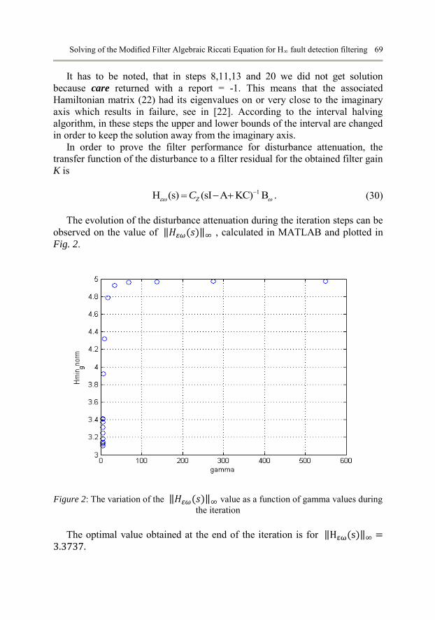
In order to prove the filter performance for disturbance attenuation, the transfer function of the disturbance to a filter residual for the obtained filter gain K is

(30)

The evolution of the disturbance attenuation during the iteration steps can be observed on the value of ‖𝐻𝜀𝜔(𝑠)‖∞ , calculated in MATLAB and plotted in Fig. 2.

Figure 2: The variation of the ‖𝐻𝜀𝜔(𝑠)‖∞ value as a function of gamma values during the iteration

The optimal value obtained at the end of the iteration is for ‖Hεω(s)‖∞ =3.3737.

1H (s) (sI A KC) B .ZC


4.3 The impact of increasing the value of 𝛾𝑚𝑖𝑛

As known, 𝛾 is a measure for the filter sensitivity [8]. In the following it is examined the impact of increasing the value of γmin .

In case if 𝛾𝑚𝑖𝑛 reached its upper limit (here 𝛾𝑚𝑖𝑛 = ∞) the term depending on 𝛾 dropped out and (9) was reduced to the form

(31)

Table 1: The impact of increasing the value of 𝛾𝑚𝑖𝑛

gamma matrix K Eigenvalues of Q

( )H s

𝛾𝑚𝑖𝑛 257.2236 -39.2216 -0.0000 -39.2216 699.2298 0.0000 -0.7934 1.6744 0.0000

0.0875 253.7718 702.6875

3.4047

10 𝛾𝑚𝑖𝑛 13.5339 -39.8412 0.0000 -39.8412 330.4657 0.0000 -0.2148 0.2480 0.0000

0.0017 8.6061 335.3976

4.9492

100 𝛾𝑚𝑖𝑛 13.4326 -39.6856 0.0000 -39.6856 329.3445 0.0000 -0.2129 0.2461 0.0000

0.0017 8.5275 334.2637

4.9717

determinist. Kalman Filter

13.4328 -39.6857 0.0000 -39.6856 329.3445 0.0000 -0.2129 0.2461 0.0000

0.0017 8.5275 334.2637

4.9719

The magnitude of the transfer functions of the disturbance to a filter residual for increased 𝛾𝑚𝑖𝑛 values is shown in Fig. 3.

0.T T T

K KAQ QA QC CQ B B


Figure 3: The magnitude (maximal singular values) of transfer functions:

H𝜀ɷ (𝛾𝑚𝑖𝑛): green line , H𝜀ɷ (10 𝛾𝑚𝑖𝑛): blue line , H𝜀ɷ (100 𝛾𝑚𝑖𝑛): red line

As it can be seen in Table 1, the smallest value for ‖𝐻𝜀ɷ (𝑠)‖∞ is 3.4047

(10.6415 dB) so the best filter sensitivity against worst case disturbance can be achieved in case of 𝛾𝑚𝑖𝑛 as it is shown in Fig.3.

In case of 100 𝛾𝑚𝑖𝑛 and the deterministic Kalman-filter there exists no significant difference between the magnitudes of the transfer functions, as it can be seen in Fig.3 (blue and red lines). For 100 𝛾𝑚𝑖𝑛 we get a ‖𝐻𝜀ɷ (𝑠)‖∞ = 4.9717 (13.93 dB), which results in lower disturbance attenuation.

It can be concluded, that the more the value of 𝛾𝑚𝑖𝑛 is increased, the less filter sensitivity can be achieved. In this sense, getting an optimal 𝛾𝑚𝑖𝑛 value is of great importance.

It is conceivable, that the H-infinity filter becomes a deterministic Kalman- filter by reaching its upper limit at 𝛾𝑚𝑖𝑛 = ∞. This can be also proven easily based on (31).

Of course, the H-infinity filter ensures that the energy gain from the disturbances to the estimation error is always less than a pre-specified level 𝛾2. Thus it is less conservative than the deterministic Kalman-filter. This is its main advantage from designer’s point of view.


4.3 Verification of the solution obtained for the MFARE via the Hamiltonian-

matrix

It is possible to verify the solution for the decision variable also via calculating the eigenvectors of the Hamiltonian-matrix of MFARE as it was explained in Subsection 3.1.

The resulting Hamiltonian-matrix for MFARE in case of γmin = 4.9698 is

5

-0.0001 0.0005 0.0000 0.0000 0.0000 0.0000 0.0000 -0.0016 0.0000 0.0000 0.0000 0.00000.0003 0.0000 -0.0001 0.0000 0.0000 0.0003

10 -0.0228 0.2229 0.0000 0.0001 -0.0.2229 -2.1747 0.0000 0.0000 0.0000 0.0000

H .0000 -0.0003

-0.0005 0.0016 0.00000.0000 -0.0000 0.0001

At first we calculate the eigenvalues and the corresponding eigenvectors of

the Hamiltonian-matrix via a similarity transformation. The resulting matrix, containing the eigenvalues is

Secondly, we have to build a (2𝑛, 𝑛) matrix 𝑉, which contains the eigenvectors of the Hamiltonian matrix corresponding to the eigenvalues with negative real parts (23).

The submatrices of V, which contain the eigenvectors, are:

Let 𝑄𝐻 denote a solution calculated using the Hamiltonian-matrix, which has a

solution

From the gamma-iteration in Subsection 4.2 we got an optimal solution as

12 1

258.0838 -32.9691 -0.7468-33.7848 691.7261 1.7722 .-0.7809 1.6763 0.0932

HQ V V

1 2

0.0005 0.0039 0.0029 0.1749 0.9986 0.8475- 0.0014 0.0001 -0.0003 , -0.9846 -0.0516 -0.5171 .0.0004 0.0062 -0.1194 -0.0027 -0.0023 -0.0139

V V

( ) 150.0393, -150.0393, 6.8273, 0.4622, -0.4622, -6.8273 .idiag H diag

257.2236 .2216.2216 699.2

-39 -0.7934-39 .6744 .-0.

298 1 .6744 7934 1 0.0934

Q


It can be stated , that matrices 𝑄𝐻 and Q are slightly different. This leads to the conclusion of plausibility of an optimal solution Q obtained by the gamma- iteration.

4.4 Solution for the MFARE by LMI

In Section 3 we introduced the method for finding the optimal solution for MFARE implemented analytically as an interval halving algorithm. However, the task of minimization results in the task of computing a system of matrix equations which is not always convex [8].

Thus, let us now consider the problem of finding the optimal solution for the filter gain by solving of MFARE formulated as a LMI.

To handle it, several commercial software tools can be chosen. In this study the LMI Control Toolbox of MATLAB has been used, which provides a set of convenient functions to solve problems involving LMIs [23].

Generally, the solution of LMIs is carried out in two stages in MATLAB. At first, the decision variables of the LMI are defined, then it is defined the system of LMIs based on these decision variables. These are mostly represented in matrix form. In the second stage, the optimization problem is solved numerically using the chosen solvers as it is explained in Section 2.

In our case study the LMI in (21) is formulated as a linear objective minimization problem. That is, the task is to minimize a linear function of 𝑥 subject to an LMI constraint:

(32)

The LMI for the MFARE derived in Section 2 is described in (21). In the following it is presented the MATLAB script for the linear objective

minimization problem of the MFARE

min : ( ) 0 .T

xc x F x

% matrices of the proposed LTI-system

A=[ -5.2643, 4.7316, 28.5021; 50.7697, -156.9827, 0; 0 , 0.4287, -9.0909 ];

B=[1.6111e+009, 0, 0; -1.5720e+010, 8.3514e+004, 146083000; 0, -141.6784, 0];

C=[1, 0 ,0 ; 0, 1, 0 ; 0, 0, 3.924e-005]; Cz=[5, 0, 0; 0 ,5, 0; 0, 0, 25];

Bd=[-47.7946 0 0 ; 466.3408 0 0 ; 0 0 0 ];

I=eye(3);

% specifying the matrix variables of the LMI

setlmis([]);

R = lmivar(1, [size(A, 1) 1]);

% constructing the system of the LMI

gamma2 = lmivar(1, [1, 1]);


lmiterm([1, 1, 1, R], 1, A, 's'); % R’A+AR

lmiterm([1, 1, 1, 0], -C'*C); % -C’C

lmiterm([1, 2, 1, 0], Cz); % Cz

lmiterm([1, 2, 2, gamma2], -1, I); % -gamma^2I

lmiterm([1, 2, 3, 0], 0); % 0

lmiterm([1, 3, 1,R], Bd', 1); % Bd’R

lmiterm([1, 3, 2, 0], 0); % 0

lmiterm([1, 3, 3, 0], -1); % -I

lmiterm([-2, 1, 1,R], 1, 1);

lmiterm([-3, 1, 1, gamma2], 1, 1);

% obtaining the system of the LMI

lmimingfilt5 = getlmis;

c = mat2dec(lmimingfilt5, zeros(size(A, 1), size(A, 1)), 1);

% the relative accuracy of the solution

options = [1e-3 , 0, 0, 0, 0];

% solving LMI

[alpha, popt] = mincx(lmimingfilt5, c, options);

% the optimal value for the decision variable "R"'

Ropt = dec2mat(lmimingfilt5, popt, R);

% the optimal value of the gamma

gopt = dec2mat(lmimingfilt5, popt, gamma2);

% the obtained γmin

gammaopt=sqrt(gopt)

% the optimal solution of the LMI

Qopt = inv(Ropt);

% the calculated filter gain

K = Qopt*C'


4.5 Comparison of the performance of the LMI with the performance of the

gamma-iteration

The efficiency and robustness of the optimal solution are interesting aspects of the fault detection filtering problem. Thus, two different methods for solving MFARE are compared, namely the LMI formulated as a linear objective minimization problem and the numerically implemented gamma-iteration.

The results of the MATLAB simulations are shown in Table 2.

Table 2: Comparison of the different solutions for the MFARE

Performance LMI as an linear objective minimization problem gamma-iteration

𝛾𝑚𝑖𝑛 4.9704 4.9698

K 278.80 -52.70 0.0000 -52.70 1308.4 0.0000 -0.500 0.600 0.0000

257.2236 -39.2216 0.0000 -39.2216 699.2298 0.0000 -0.7934 1.6744 0.0000

Eigenvalues of Q

0.3 276.1 1311

0.0017 8.5275 334.2637

‖𝐻𝜀𝜔(𝑠)‖∞

4.4345 3.4047

number of iterations

9 21

computation cost (sec)

0.1 1

From the simulation and results of the comparison of the two different

methods it can be concluded that each one gives an optimal solution. To be more precise, the minimization algorithm has been applied until the satisfaction of the positive definiteness. As it can be seen in Table 2, the smallest 𝛾𝑚𝑖𝑛 value could be reached using the simple gamma-iteration, but the result obtained this way is just slightly different from the result obtained using LMI. However, the higher filter gain obtained in case of LMI suggests that the filter may be faster but less effective against disturbance. On other hand the burden of successive numerical computation of the quadratic matrix equality resulted in a significant computation cost. It has disadvantages despite its simplicity. From the results it is visible that modern computation methods as LMI are more capable to handle such complex mathematical problems as the solution of the MFARE. From the results mentioned above, it is conceivable that LMI-s are effective and powerful tools for handling complex but standard problems such as rapidly computing of a global optimum with some specified accuracy.


The technique of gamma-iteration, despite its slowness, is easy to be handled. Concretely it gives more flexibility to examine the solution for MFARE. For example, it is easy to analyze the impact of the gamma value on the number of iteration steps or the impact of changing of the disturbance on the optimal solution.

One can easily perform experiments and get answers e.g. to the following questions: How does the iteration converge? How do the eigenvalues of the decision variable change? How close are they to the imaginary axis? How are they distributed? How does the filter gain change by reduction of the value of gamma? All these issues can be easily examined, step by step during the iterations.

4. Conclusion

In our paper we performed a benchmark based on collected concepts for solutions of MFARE by conventional gamma-iteration and LMI. From the simulation results of LMI, it can be concluded that it is well capable for computing the global optimum of the quadratic cost function rapidly with some specified accuracy even if this is to be done in the case of MFARE. Both methods, i.e. the gamma-iteration and the LMI formulation as a linear objective minimization problem, are capable for solution of MFARE. Moreover, they deliver only slightly different results. However, the LMI leads to an optimal solution faster, in about 100ms.

The analytically implemented gamma-iteration, despite its slowness, gives much more flexibility to examine the minimization process. For example, it is easy to examine the impact of the iteration steps or the impact of changing of the disturbance on the optimal solution. For this reason we propose the use of both approaches, that is, using the gamma-iteration in the preliminary stage in order to perform an analysis and using LMI in the stage of the synthesis to perform the implementation. Our further work will include an extension of our LMI approach to a switched linear system.

References

[1] Edelmayer, A., Bokor, J., Keviczky, L., “An H∞ Filtering Approach to Robust Detection of Failures in Dynamical Systems”, in Proc. 33th Annual Decision and Control, Conf., pp. 3037-3039, Buena Vista, USA, 1994.

[2] Edelmayer, A., Bokor, J., Keviczky, L., “An H∞ Filter Design for Linear Systems: Comparison of two Approaches” IFAC 13th Triennial World Congress, San Francisco,

USA, 1996.


[3] Yaesh, I. , Shaked, U., “ Game Theory Approach to Optimal Linear State Estimation and Its Relation to the Minimum H∞ -norm Estimation”, IEEE Trans. Aut. Control, AC-37(6), pp. 828-831, 1992.

[4] Chen, J., Patton, R. J., “Robust Model-Based Fault Diagnosis for Dynamic Systems”, First Edition, Springer Science & Business Media, New York, 1999.

[5] Matusu, R., “Linear Matrix Inequalities and Semidefinite Programming: Applications in Control”, Internal Journal of Mathematical Models and Methods in Applied Sciences, Vol. 8, 2014.

[6] Gahinet, P, Apkarian, P., “A linear matrix inequality approach to H∞ control”, International Journal of Robust and Nonlinear Control, Vol. 4, pp. 421–448, 1994.

[7] Iwasaki, T., Skelton, R. E., “All controllers for the general H∞ control problem: LMI existence conditions and state space formulas”, Automatica, Vol. 30, pp. 1307–1317, 1994.

[8] Edelmayer A., “Fault detection in dynamic systems: From state estimation to direct input reconstruction”, Universitas-Győr Nonprofit Kft., Győr, 2012.

[9] Chong, E., K., P., Zak, S., H., “An Introduction to Optimization”, 4th Edition, Wiley, New Jersey, 2013.

[10] Ostertag, E., “Mono- and Multivariable Control and Estimation: Linear, Quadratic and LMI Methods” , Matematical Engineering, Vol.2, Springer, Berlin, Heidelberg, 2011.

[11] Ankelhed, D., “On the design of low order H∞ controllers”, Ph.D. These, Linköping University, Linköping, 2011.

[12] Duan, G., R., Yu, H., H., “LMIs in Control Systems: Analysis, Design and Applications”, CRC Press, Boca Raton, 2013.

[13] Boyd, S., Ghaoui, L. E., Feron, E., and Balakrishnan, V., “Linear Matrix Inequalities in System and Control Theory”, SIAM, Philadelphia, 1994.

[14] Bokor, J., Gáspár, P., Szabó, Z., “ Robust Control Theory“, Typotex, Budapest, 2013. [15] Lunze, J., “Regelungstechnik 2 – Mehrgrößensysteme, Digitale Regelung“, Springer, 7.

Auflage, 2013. [16] Jankovic, M., Kolmanovsky, I., “Robust Nonlinear Controller for Turbocharged Diesel

Engines”, Procedings of the American Control Conference, Philadelphia, 1998. [17] Jung, M., “Mean-value modelling and robust control of the airpath of a turbocharged diesel

engine”, Ph.D. These, University of Cambridge , 2003. [18] Horvath, Zs., Edelmayer, A., “LTI-modelling of the Air Path of Turbocharged Diesel

Engine for Fault Detection and Isolation”, Mechanical Engineering Letters, Vol. 14, pp. 172-188, Gödöllő, 2016.

[19] Herceg, M., “Nonlinear Model Predictive Control of a Diesel Engine with Exhaust Gas Recirculation and Variable Geometry Turbocharger”, Diploma Thesis, Slovak University of Technology in Bratislava, Bratislava, 2006.

[20] Yung, C. F., “Reduced-order H∞ controller design: An algebraic Riccati euqation approach”, Automatica, Vol. 36, pp. 923–926, 2000.

[21] Lanzon, A., Feng, Y., Anderson, B.,D.,O. and Rotkowitz, M., “ Computing the Positive Stabilizing Solution to Algebraic Riccati Equations With an Indefinite Quadratic Term via a Recursive Method”, IEEE Trans. Aut. Control, Vol. 53, pp. 2280–2291, NO. 10. November, 2008.

[22] https://de.mathworks.com/help/control/ref/care.html?requestedDomain=www.mathworks.com

[23] Gahinet, P., Nemirovski, A., Laub, A.J., and Chilali, M., “ LMI Control Toolbox for Use with Matlab”, The MathWorks, Natick, Messachusetts, 1995.

http://eu.wiley.com/WileyCDA/Section/id-302479.html?query=Edwin+K.+P.+Chong

http://eu.wiley.com/WileyCDA/Section/id-302479.html?query=Stanislaw+H.+Zak

https://rd.springer.com/search?facet-creator=%22Eric+Ostertag%22

https://de.mathworks.com/help/control/ref/care.html?requestedDomain=www.mathworks.com

https://de.mathworks.com/help/control/ref/care.html?requestedDomain=www.mathworks.com

solving of the modified filter algebraic riccati equation ... · solving of the modified filter...

Documents