Research Division Federal Reserve Bank of St. Louis Working Paper Series

Solving Linear Difference Systems with Lagged Expectations by a Method of Undetermined Coefficients

Pengfei Wang and

Yi Wen

Working Paper 2006-003C http://research.stlouisfed.org/wp/2006/2006-003.pdf

January 2006 Revised May 2006

FEDERAL RESERVE BANK OF ST. LOUIS Research Division

P.O. Box 442 St. Louis, MO 63166

______________________________________________________________________________________

The views expressed are those of the individual authors and do not necessarily reflect official positions of the Federal Reserve Bank of St. Louis, the Federal Reserve System, or the Board of Governors.

Federal Reserve Bank of St. Louis Working Papers are preliminary materials circulated to stimulate discussion and critical comment. References in publications to Federal Reserve Bank of St. Louis Working Papers (other than an acknowledgment that the writer has had access to unpublished material) should be cleared with the author or authors.

Solving Linear Di¤erence Systems with Lagged Expectationsby a Method of Undetermined Coe¢ cients�

Pengfei WangDepartment of Economics

Cornell University

Yi WenResearch Department

Federal Reserve Bank of St. Louis

(This version: May 2006)

Abstract

This paper proposes a solution method to solve linear di¤erence models with lagged expec-

tations in the form of

AEtSt+1 +NPi=1

�iEt�iSt+1 = BSt +NPi=1

�iEt�iSt + CZt;

where N is the order of lagged expectations. Variables with lagged expectations expand the

model�s state space greatly whenN is large; and getting the system into a canonical form solvable

by the traditional methods involves substantial manual work (e.g., arranging the state vector St

and the associated coe¢ cient matrices to accommodate Et�iSt, i = 1; 2; :::; N), which is prone to

human errors. Our method avoids the need of expanding the state space of the system and shifts

the burden of analysis from the individual economist/model solver toward the computer. Hence

it can be a very useful tool in practice, especially in testing and estimating economics models

with a high order of lagged expectations. Examples are provided to demonstrate the usefulness

of the method. We also discuss the implications of lagged expectations on the equilibrium

properties of indeterminate DSGE models, such as the serial correlation properties of sunspots

shocks in these models.

Keywords: Undetermined Coe¢ cients, Linear Di¤erence System, Lagged Expectations, La-

bor Hoarding, Sticky Information, Indeterminacy, Serially Correlated Sunspots.

JEL Codes: C63, C68, E30, E40.

�Matlab programs used in this paper are available at our web sites. We thank John McAdams for excellent researchassistance. The views expressed in the paper and any errors that may remain are the authors�alone. Correspondence:Yi Wen, Research Department, Federal Reserve Bank of St. Louis, St. Louis, MO, 63144. Phone: 314-444-8559.Fax: 314-444-8731. Email: yi.wen@stls.frb.org.

1

1 Introduction

The standard methods of solving linear rational expectations models deal with the linear di¤erence

system,

AEtSt+1 = BSt + CZt; (1)

where S is a vector of endogenous variables, Z is a vector of exogenous forcing variables, and Et

denotes the expectation operator based on information available up to period t. Linear rational

expectations models with lagged expectations take the form,

AEtSt+1 +

NXi=0

�iEt�iSt+1 = BSt +NXi=1

�iEt�iSt + CZt; (2)

which di¤ers from system (1) by the lagged expected variables, Et�iSt (i > 0). Thus, system (2) is

more general than system (1).

Linear di¤erence systems with lagged expectations are becoming increasingly popular as a way

to characterize economic behaviors in macroeconomics. For example, lagged expectations exist

in DSGE models when some choice variables in period t must be determined N > 0 periods

in advance, or be based on information available N periods earlier, before the current economic

shocks are realized in period t. This type of model includes the labor hoarding model of Burnside,

Eichenbaum, and Rebelo (1993) and the sticky-information model of Mankiw and Reis (2002).

To directly apply the traditional solution methods, such as that of Blanchard and Kahn (1980),

King and Watson (1998), Christiano (2002), or Klein (2000) and Sims (2002), to solve system (2)

requires expanding the state vector St to include Et�iSt (i = 1; 2; :::; N) as additional state variables.

This is not a trivial task, especially when N is large. For example, in the sticky-information model

of Mankiw and Reis (2002), N = 1. Notice that the state variables with lagged expectations arenot predetermined variables, hence they must also be solved for in equilibrium. An example of

solving a DSGE sticky-information model directly by traditional method can be found in Andrés,

López-Salido, and Nelson (2005). Because of the inconvenience of traditional method, these authors

have to restrict the order of lagged expectations to be N = 4. This arbitrary truncation may su¤er

from accuracy problems and can severely distort a model�s true underling dynamics.

This paper proposes an alternative method to solve linear di¤erence systems with lagged expec-

tations such as system (2). The solution method is a combination of the method of undetermined

coe¢ cients discussed in Taylor (1986) and the traditional methods based on Blanchard and Kahn

(1980). Our method treats the order of lagged expectations N as a free parameter and is easy

2

to implement. Under this method the dimension of the state space in system (2) is exactly the

same as that in system (1). Thus there is no need to expand the state space of system (1) in the

presence of lagged expectations. This method is also simpler than that used by Taylor because in

our method there is no need to determine the entire in�nite sequence of coe¢ cients in the MA(1)representations of the decision rules.

The key of the method is to convert any lagged expected variables, Et�iSt, into i-step ahead

forecast errors, St�Et�iSt. Since in equilibrium, St always has the moving average representation,St =

P1j=0�j"t�j ; where " is a vector of i:i:d innovations in the exogenous forcing processes Zt,

the i-step ahead forecast error is given by St � Et�iSt =Pi�1j=0�j"t�j ; which is a �nite moving

average process and is much easier to handle than the expected variables Et�iSt+l. Thus, system

(2) can be converted into system (1) easily with just a �nite number of undetermined coe¢ cient

matrices f�jgNj=0. This is an easier task (especially when N is large) since getting the system (2)

into a form solvable directly by the traditional methods may involve substantial manual work, as

expanding the state vector St and changing the associated coe¢ cient matrices to accommodate

Et�iSt (i = 1; 2; :::; N) cannot be done mechanically by computers and is hence prone to human

errors, whereas our method shifts the burden of analysis from the individual economist/model

solver toward the computer.

In this paper, we also consider several examples to illustrate the usefulness of our method in solv-

ing DSGE models with lagged expectations. In particular, we show how serially correlated sunspots

shocks (in contrast to the i:i:d sunspots shocks) can be introduced into the Benhabib-Farmer (1994)

model via lagged expectations. This example refutes a popular notion in the indeterminacy lit-

erature that introducing predetermined variables or dynamic adjustment costs in capital or labor

necessarily eliminates sunspots equilibria in the Benhabib-Farmer model.

2 The Method of Undetermined Coe¢ cients

LetXt = [x1t; x2t; :::; xpt]0 be a vector of non-predetermined variables in period t, let Yt = [y1t; y2t; :::yqt ]

0

be a vector of predetermined variables in period t; and let Zt = [z1t; z2t; :::; zmt]0 be a vector of ex-

ogenous forcing variables with the law of motion given by Zt = �Zt�1 + "t; where � is a stable

m � m matrix and " is an m � 1 vector of othorgonal i:i:d: innovations with realization in the

beginning of period t. Let St = [X 0t; Y

0t ; Z

0t]0 and let k = p+ q +m. A rational expectations DSGE

model with lagged expectations can always be reduced to the following log-linear di¤erence system:

AEtSt+1 +

NXi=1

�iEt�iSt+1 = BSt +NXi=1

�iEt�iSt; (3)

3

where fA;B;�i;�ig are k � k coe¢ cient matrices.The corresponding system without lagged expectations is given by

~AEtSt+1 = ~BSt; (30)

where ~A =�A+

PNi=1 �i

�; ~B =

�B +

PNi=1 �i

�: Thus, a solution exists for system (3) if and only

if a solution exists for system (30). In other words, the eigenvalues of system (3) and system (30)

are identical. This can be seen by taking expectations on both sides of (3) based on Et�N to get

~AEt�NSt+1 = ~BEt�NSt: (300)

If S�t is a stationary solution for equation (3), then Et�NS�t must also be stationary and hence it

must constitute a solution for equation (300). On the other hand, if Et�NS�t is a stationary solution

for equation (300), then S�t must also be stationary and hence it must constitutes a solution for

equation (3).

An implication of this is that letting some variables be predetermined in a DSGE model, such

as via labor hoarding or sticky information, will not a¤ect the equilibrium properties of the model

in terms of the existence and multiplicity of equilibria. For example, if the original model without

labor hoarding (or sticky-information) has a unique equilibrium, then introducing labor hoarding

(or sticky information) has no e¤ect on the uniqueness of the equilibrium. Similarly, if the model

without labor hoarding (or sticky information) is indeterminate, then introducing labor hoarding or

sticky-information will not eliminate indeterminacy. This also implies that linear sunspots shocks

to expectation errors do not have to be i:i:d processes in indeterminate DSGE models once lagged

expectations are introduced. Linear sunspots shocks can be serially correlated processes under

lagged expectations. The order of the serial correlations of sunspots are determined by the order

of lagged expectations in the indeterminate model. An example is provided in the next section.

Our method of undetermined coe¢ cients constitutes the following steps:

Step 1. Replace the lagged expected variables (Et�iSt) by the forecast errors (St�Et�iSt) withundetermined coe¢ cients f�jg.

Since the solution for St can always be expressed as a moving average process, St =P1i=0�i"t�i;

where �i are undetermined k�m matrices, we have St�Et�iSt =Pi�1j=0�j"t�j ; for i = 1; 2; :::; N:

1

Adding well de�ned zeros, (St+1 � St+1) and (St � St), to Equation (3) and re-arranging terms, wehave

~AEtSt+1 +

NXi=1

�i (Et�iSt+1 � EtSt+1) = ~BSt +

NXi=1

�i (Et�iSt � St) ; (4)

1Note that the forecast errors for the exogenous forcing vector Zt are known, hence we only need to determine asubset of the elements in �i.

4

where ~A =�A+

PNi=1 �i

�; ~B =

�B +

PNi=1 �i

�: Substituting out the j-step ahead forecast errors

by their corresponding moving average processes with undetermined coe¢ cients gives

~AEtSt+1 �

NXi=1

�i

!�1"t �

NXi=2

�i

!�2"t�1 � :::� �N�N"t�N+1

= ~BSt �

NXi=1

�i

!�0"t �

NXi=2

�i

!�1"t�1 � :::� �N�N�1"t�N+1: (40)

Notice that we only need to determine the �nite sequence of undetermined coe¢ cients, f�0;�1; :::;�Ng,

instead of the in�nite sequence of undetermined coe¢ cients, f�ig1i=0. De�ne ~�j =PNi=j �i and

~�j =PNi=j �i. Equation (4

0) becomes

~AEtSt+1 = ~BSt + [�1 � 0] �t; (400)

where

� ��~�1 ~�2 � � � ~�N

�k�Nk ; �

�~�1 ~�2 � � � ~�N

�k�Nk ;

1 �

266664�1 0 � � � 0

0 �2. . .

......

. . . . . . 00 � � � 0 �N

377775Nk�Nm

; 1 �

266664�0 0 � � � 0

0 �1. . .

......

. . . . . . 00 � � � 0 �N�1

377775Nk�Nm

�t ��"0t; "

0t�1; :::; "

0t�N+1

�0Nm�1 ;

where the subscript outside each square parentheses denotes the dimension of the matrix. The

white noise vector �t has the following law of motion:

�t+1 = ��t +

�Im0

�"t+1; (5)

where Im is an m�m identity matrix and

� �

266666664

0 0 � � � � � � 0

Im 0. . . . . .

...

0 Im. . . . . .

......

. . . . . . 0 00 � � � 0 Im 0

377777775Nm�Nm

;

which has the property of �j = 0 for j � Nm.

5

Step 2. Solve equation (400).

Notice that equation (400) is a standard system without lagged expectations. Hence we can solve

the system with standard methods such as that proposed by Blanchard and Kahn (1980), King

and Watson (1998), Christiano (2002), or Klein (2000) and Sims (2002).2 The solution is a set of

decision rules of the form

Xt = Hy

�YtZt

�+H�()�t; (7)

�Yt+1Zt+1

�=My

�YtZt

�+M�()�t +

�0Im

�"t+1; (8)

where � (�1 � 0). It can be shown that H�() and M�() depend linearly on the

undetermined coe¢ cient matrix and that Hy and My do not depend on .

Step 3. Solve for f�0;�1; :::;�Ng :

Denote as the expanded state vector Qt ��Y 0t Z 0t �0t

�0. The equilibrium decision rules and

laws of motion (7)-(8) can be expressed as

Xt = H()Qt (70)

Qt+1 =M()Qt +G"t+1: (80)

Hence, the forecast errors are given by

Qt � Et�iQt = G"t +M()G"t�1 + :::+Mi�1()G"t�i+1 (9)

=i�1Xj=0

M j()G"t�j ;

Xt � Et�iXt = H() [Qt � Et�iQt] (10)

= H

i�1Xj=0

M j()G"t�j ;

for i = 0; 1; 2; :::; N � 1: Equation systems (9) and (10) can be stacked into the following form after

leaving out the exogenous variables �t from the bottom rows in equation system (9):

24 XtYtZt

35� Et�i24 XtYtZt

35 = i�1Xj=0

Pj()"t�j : (11)

2Our method is completely di¤erent from that of Christiano (2002). Christiano�s method of undetermined coe¢ -cients does not involve transforming variables with lagged expectations (Et�iSt) to the corresponding forecast errors(St � Et�iSt).

6

By de�nition (4) we also have

24 XtYtZt

35� Et�i24 XtYtZt

35 = i�1Xj=0

�j"t�j : (12)

Recall that = (�1 � 0) is a super matrix with �j (j = 0; 1; :::; N) as its elements. Clearly,

the equivalence of representation (11) and representation (12) constitutes N �m equations with

(N + 1)�m unknowns in f�jgNj=0. An extra equation is found by updating equations (11) and (12)

by one period forward and then taking expectation based on Et. In particular, for i = 1; 2; :::N +1,

term-by-term comparison between (11) and (12) for all of the coe¢ cients of "t�i suggests that

P0(�1 � 0) = �0

P1(�1 � 0) = �1

... = ... (13)

PN (�1 � 0) = �N�1

PN+1(�1 � 0) = �N ;

where the last equation in (13) is derived by updating (11) and (12) by one period forward and

then taking expectation based on Et. System (13) can be compactly expressed as

P () = : (14)

The solution for the sequence f�igNi=0 can thus be found as a �xed point for equation (14). Although

analytical solutions for equation (14) exist, it can also be solved numerically using standard packages

in Gauss or Matlab. In particular, since (14) is a linear mapping, the existence of an analytical

solution and the fast speed of convergence under numerical iterations are guaranteed. The linear

property of the function P () is established by the following proposition:

Proposition 1 Pj() is linear in for all j.

Proof. See the Appendix.

In the next section we consider several examples to illustrate the usefulness of our method of

undetermined coe¢ cients for solving linear di¤erence systems with lagged expectations.

7

3 Examples

3.1 The Mankiw-Reis Model in General Equilibrium

DSGE models with sticky information have also been studied by Keen (2004) and Trabandt (2005),

among others.3 A version of the model is described as follows. A representative household in the

model chooses consumption (c), labor (n), investment (i), money holdings (M), and bond holdings

(B) to solve

maxE0

1Xt=0

�t

c1� t � 11� � a n

1+ nt

1 + n

!

subject to

(Mt+1 +Bt+1) =Pt + (ct + it) � wtnt + qtkt + �t + (Mt +Xt +Rt�1Bt) =Pt; (15)

ct + it � (Mt +Xt) =Pt; (16)

where it = kt+1 � (1 � �)kt denotes investment. The budget constraint (15) implies that the

household begins in period t with initial levels of money, Mt, bonds, Bt, capital, kt, real pro�ts

(dividends), �t, and the wage and rental payment, wtnt + qtkt; from �rms, where Rt is the gross

nominal interest rate, wt is the real wage rate, Pt is the aggregate price level, and qt is the real

rental rate of capital. Xt represents money injection from the monetary authority. The total income

is allocated to the next period money demand, Mt+1, bond holdings, Bt+1, consumption, ct, and

investment, it. All purchases are subject to a cash-in-advance constraint (16).

Denote f�t; �tg as the Lagrangian multipliers for the budget constraint (15) and the CIA con-straint (16), the �rst order conditions of the household with respect to fct; nt; kt+1;Mt+1; Bt+1g aregiven, respectively, by

c� t = �t + �t

an n = �twt

�t + �t = �(1� �)Et��t+1 + �t+1

�+ �Et�t+1qt+1

�t=Pt = �Et��t+1 + �t+1

�=Pt+1

�t=Pt = �RtEt�t+1=Pt+1

Aggregate output is produced competitively using intermediate goods according to the technol-ogy,

3Keen (2004), however, does not discuss how his model is solved. Although Trabandt (2005) does discuss hissolution technique, his method is very di¤erent from ours.

8

y =

0@ 1Z0

y(i)��1� di

1A�

��1

;

where � > 1 measures the elasticity of substitution among the intermediate goods, y(i). Let

p(i) denote the price of intermediate good i, the demand for intermediate goods is given by y(i)

=�p(i)P

���yt; and the relationship between the �nal goods price and intermediate goods prices is

given by P =�R 10 p(i)

1��di� 11��.

Each intermediate good i is produced by a single monopolistically competitive �rm according

to the technology, y(i) = k(i)�n(i)1��. Intermediate good �rms face perfectly competitive factor

markets, and hence have the following factor demand functions for fk; ng: qt = mct�yt(i)kt(i)

; wt =

mct(1��) yt(i)nt(i); where mc =

� qt�

�� � wt1��

�1��denotes real marginal cost. In each period, a fraction

(1� �) of �rms update information about the state of the economy and set their optimal pricesaccordingly. The rest continue to set their prices based on old information. A �rm who updated

its information j periods ago maximizes its pro�ts in the current period t by solving

maxpt(j)

Et�j

�pt(j)

Pt�mct

�yt(j);

subject to the demand constraint, yt(j) =�pt(j)Pt

���yt: The optimal price is given by pt(j) =

�Et�j(P�t ytmct)

(��1)Et�j(P��1t yt): Following Mankiw and Reis, the aggregate price level is given by P = (1 �

�)hP1

j=0 �jp(j)1��

i 11��

: Log-linearizing the above two price-equations and re-arranging terms (see

Mankiw and Reis, 2002, for details), we can obtain what Mankiw and Reis called the "sticky

information Phillips Curve":

�t =1� ��mct + (1� �)

1Xj=0

�jEt�1�j(�t +�mct)]; (17)

which can be re-arranged into an equation without lagged expectations but involving only forecasterrors:

mct = �mct�1 + (1� �)1Xj=1

�j [�t +�mct � Et�j(�t +�mct)] (18)

9

In a symmetric equilibrium, k(i) = k; n(i) = n; and y(i) = y. Market clearing in the goods

and the asset markets implies c + i = y;Mt+1 = Mt + Xt; and Bt+1 = Bt = 0: The equilibrium

dynamics of the model can be approximated by the following system of log-linearized equations

(after substituting out f�; �;w; q; yg using the �rst-order conditions):

� ct = �(1� �)Et (� ct+1) + (1� �(1� �))Et (( n + 1)nt+1 � kt+1)

( n + �)nt �mct � �kt = Et (� ct+1 � �t+1)

mct = �mct�1 + (1� �)1Xj=1

�j [�t +�mct � Et�j(�t +�mct)]

scct + si

�1

�kt+1 �

1� ��kt

�= �kt + (1� �)nt

�kt + (1� �)nt � (�kt�1 + (1� �)nt�1) = xt � �t

Rt = ( n + �)nt �mct � �kt � Et (( n + �)nt+1 �mct+1 � �kt+1 � �t+1)

These equations can be arranged into a form similar to system (2) (after adding three identities,

kt = kt; nt = nt;mct = mct, and the law of motion for money growth, xt+1 = �xt + "t+1 into the

system):

AEtSt+1 = BSt +G1Xi=1

�i [St � Et�iSt] ; (19)

where St+1 = [k0; c0; �0; n0;mc0; R0; k; n;mc; x0] (note: z0 � zt+1) and G is a 10 � 10 matrix withzeros everywhere except that the fourth row is given by the row vector

(1� �)�0 0 1 0 1 0 0 0 �1 0

�:

Letting St =P1i=0�i"t�i; Equation(19) can be truncated to

AEtSt+1 = BSt +GNXi=1

�i�i�1"t�i

= BSt +G�t: (20)

Since A is singular, we use the method of King and Watson (1998) to solve Equation (20). Analysis

shows that N = 20 gives very good results. For example, setting N = 50 does not lead to noticeable

di¤erence in the impulse responses of the model.

10

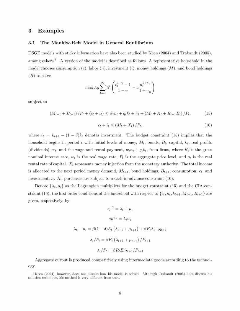
Figure 1. Impulse Responses to a Money-Growth Shock.

Impulse Responses. The time period is a quarter. In order to preserve the output-in�ation

dynamics of the Mankiw-Reis (2002) model, we set the risk aversion coe¢ cient = 0:005; and the

inverse labor supply elasticity n = 0:05. These parameter values are needed because larger values

tend to worsen the persistence of in�ation and its lagged relationship to output in the Mankiw-Reis

model. For the same reason, we also set � = 0:8; which implies that it takes the average price level

�ve quarters to fully adjust after an initial shock. We �nd that the larger � is, the more in�ation

lags output. We set the time discounting factor � = 0:99, the capital�s share parameter � = 0:2,4

the rate of depreciation � = 0:025, the elasticity of substitution parameter � = 10 (implying a

markup of about 10%) as in Mankiw and Reis. We assume that money growth follows an AR(1)

process with persistence parameter � = 0:6, which is consistent with Mankiw and Reis and much

of the sticky-price literature.5 The impulse responses of the model to a money growth shock are

graphed in Figure 1, which is generated by setting N = 30.

The left window in Figure 1 shows that after a correlated money growth shock, consumption

drops �rst before it increases. Investment, however, increases a lot in the initial periods despite the

cash-in-advance constraint. Labor and output have similar volatilities in responding to the shock.

The right window in Figure 1 shows that both output and in�ation are hump-shaped and highly

persistent after the shock. Most importantly, in�ation lags output by 3-4 quarters. This pattern of

output-in�ation dynamics has been cited by the existing literature as the litmus test for monetary

4A large value of � tends to destroy the hump-shaped and lagged in�ation dynamics. The smaller � is, the closerthe results are to those in Mankiw and Reis (2002).

5A larger value of � also tends to generate more lagged in�ation relative to output.

11

models (see, e.g., Fuhrer and Moore, 1995, Mankiw and Reis, 2002, Christiano, Eichenbaum, and

Evans, 2005, and Wang and Wen, 2005).

3.2 A Labor Hoarding Model

Consider the labor hoarding model of Burnside et al. (1993) and Burnside and Eichenbaum (1996)

in which a representative agent chooses sequences of consumption (c), probability to work (n),

e¤ort to work (e), capital utilization rate (u), and next-period capital stock (k) to solve

maxfng

Et�N

(max

fc;u;e;k0gEt

( 1Xt=0

�t��t log ct+s + nt+s log (T � � � et+sf)

+ (1� nt+s) log T

�))

subject to

ct+s + gt+s + kt+1+s ��1� �u�t+s

�kt+s � At (ut+skt+s)� (et+snt+s)1�� ;

where T is time endowment in each period, � is the cost of time from going to work and f is

the length of working hours per shift. Since the size of the labor force is normalized to one, n

also represents the employment rate. The Et�N operator indicates that employment is always

determined N � 0 periods in advance based on information available in period t � N . The keydi¤erence between this model and the model studied by Burnside and Eichenbaum is that the

number of labor hoarding periods N in this model is a free parameter, hence it can be made

arbitrarily large. As will become clear shortly, the size of N has no e¤ect on the model�s state

space under our method of undetermined coe¢ cients.

If the time period is a quarter, than the labor hoarding period N may be around 1� 4 quartersbased on the U.S. data. However, if the time period is a month or a day, then N can become quite

large. The literature has shown that due to consistence in parameter calibrations, quarterly time

series generated from a daily model by aggregation may di¤er substantially from those generated

from the corresponding quarterly model. This is especially the case for employment dynamics (see,

e.g., Aadland, 2001; and Aadland and Huang, 2004). As pointed out by Aadland and Huang (2004),

in reality, actual decisions by economic agents are likely to be made at time intervals that are more

frequent than the intervals at which economic data are sampled. Hence, in practice, it may be

necessary for researchers to solve labor hoarding models at daily or monthly frequency and then

convert the times series into quarterly or annual frequency, which would involve solving models

with a large value of N .

If N > 0, adjusting employment stock is not instantaneous in the model. But the e¤ort level

e (or utilization rate of labor) and the utilization rate of capital can be adjusted instantaneously,

re�ecting the idea of factor hoarding (Burnside et al., 1993). The rate of capital depreciation,

12

�u�t ; is time dependent in this model, re�ecting costs associated with the capital utilization rate

(� > 1). The random variable �t represents aggregate impulses shifting the marginal utilities of

agents�consumption by creating urges to consume, gt is shocks to government spending, and At is

shocks to technology. All shocks follow stationary AR(1) processes:

log �t = (1� ��)�� + �� log �t�1 + "�t; "�t � N(0; �2�);

log gt = (1� �g)�g + �g log gt�1 + "gt; "gt � N(0; �2g);

logAt = (1� �a) �A+ logAt�1 + "at "at � N(0; �2a);

where the innovations f"�t; "gt; "atg are assumed to be othorgonal to each other.

The �rst-order conditions with respect to fn; c; u; e; kg are given respectively by:

Et�N�log T � log (T � � � etf)� (1� �)�tAt (utkt)� e1��t n��t

= 0

�tct= �t

At�u��1t k�t (etnt)

1�� = ��u��1t kt

fntT � � � etf

= (1� �)�tAt (utkt)� e��t n1��t

�t = �Et

n�t+1

h�At+1u

�t+1k

��1t+1 (et+1nt+1)

1�� + 1� �u�t+1io

ct + gt + kt+1 ��1� �u�t

�kt = At (utkt)

� (etnt)1�� :

The model�s equilibrium is characterized by linear approximations around the steady state. Using

circum�ex variables to denote log deviations from steady state values, where the steady state

refers to the model economy�s stationary point in the absence of random shocks (e.g., all variables

including the exogenous shocks are constant), the log-linearized �rst-order conditions are given by:6

Et�NnAt + �t + �

�ut + kt

�� � (et + nt)

o= 0 (21)

�t � ct = �t

At + (1� �)�et + nt � kt

�= (�� �) ut

6Note that the �rst-order conditions with respect to nt and et imply that in the steady state,

1

log T � log (T � � � �ef) =�ef

T � � � �ef :

13

�et = At + �t + ��ut + kt

�� � (et + nt)

�t = Et

��t+1 +

�

1� �At+1 � ��ut+1 + kt+1

�+ � (et+1 + nt+1)

�

scct + sg gt +si��kt+1 = At +

��+ si

1� ����

�kt + (�� si�) ut + (1� �) (et + nt) ;

where � � �efT����ef ; � �

�1� �

�1� ��z

��(1� �) ; and sc + si + sg = 1 represent the steady-state

ratios of consumption, investment and government spending with respect to output, and �� is the

steady-state capital depreciation rate. The important steady-state relationships that help determine

the steady-state values and the elasticity of depreciation cost (�) are implied by the �rst order

conditions of the model, which are given respectively by

�k�y =

��

1��(1���); si = ��

�k�y ; sc = 1� si � sg; � =

1��(1���)���

; �� = ��u�:

To solve the model, denote Zt = [ct; nt; et; ut]0 as the control vector, St =

hkt; �t; At; �t; gt

i0as

the expanded state vector, and denote the forecast errors as Zt �Et�NZt =PN�1j=0 �

zj"t�j � z�t,

and St � Et�NSt =PN�1j=0 �

sj"t�j � s�t. In equation (21), replace all variables with lagged

expectations by their corresponding forecast errors (notice that nt � Et�N nt = 0 because labor isdetermined in period t�N). Equation (21) then can be written as:

A1Zt = B1St + (A1z �B1s) �t; (22)

where A1 =�0 � � ��

�; and B1 =

�� 1 1 0 0

�: The �rst-order conditions can then

be represented by the following linear di¤erence system

Zt = HsSt +H�()�t; (23)

EtSt+1 =MsSt +M�()�t; (24)

which can be solved by standard methods as discussed in the previous section.

Impulse Responses. The time period is a quarter. In calibrating the parameter values for a

quarterly model, we follow Burnside and Eichenbaum (1996) by setting T = 1; 369 per quarter,

� = 60; and f = 324:8 (implying a steady-state e¤ort level �e = 1). We also set the discounting

factor � = 0:99; the capital�s elasticity � = 0:36, the steady-state government-spending to output

ratio sg = 0:2, and the steady-state quarterly rate of capital depreciation �� = 0:025 (implying 10

percent a year and � � 1:4). These parameter values imply �k�y = 8:5 (in a quarter or 2:1 in a year)

14

and si � 0:2. There is no need to pin down the steady-state capital utilization rate since � can

always be chosen so that �u matches the data. We assume �� = �g = �a = 0:9.

Figure 2. Impulse Responses to a Government-Spending Shock.

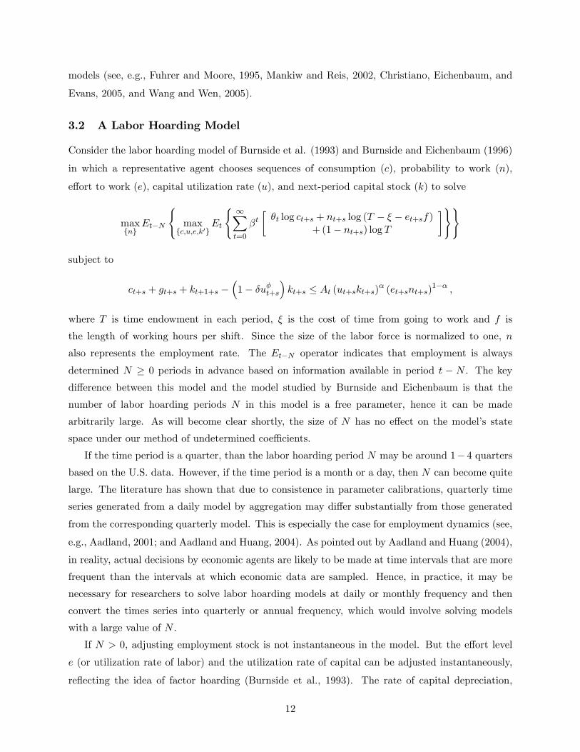
As an example, the impulse responses of the model economy to a one-standard-deviation shock

to government spending are graphed in Figure 2, where the labor hoarding period is set at N =

10 quarters. The left window shows that the volatility of the economy is substantially smaller

during the period of labor hoarding than that after employment becomes �exible ten quarters

later. Other than that, the model behaves similar to a standard RBC model. The right window

shows that labor�s productivity is procyclical during the period of labor hoarding, which is due

to the movements in e¤ort and capacity utilization. But as soon as labor becomes �exible ten

quarters later after the shock, the e¤ort level returns to zero and productivity becomes counter-

cyclical. Figure 3 reports the impulse responses when N = 50. It shows that labor becomes

essentially constant even after the hoarding period has ended, and its role in the business cycle

is replaced by e¤ort and capacity utilization during the periods of labor hoarding. This tends to

reduce the volatility of output even further compared to the case of N = 10. Thus, the longer the

labor hoarding period is, the less volatile the economy is.

15

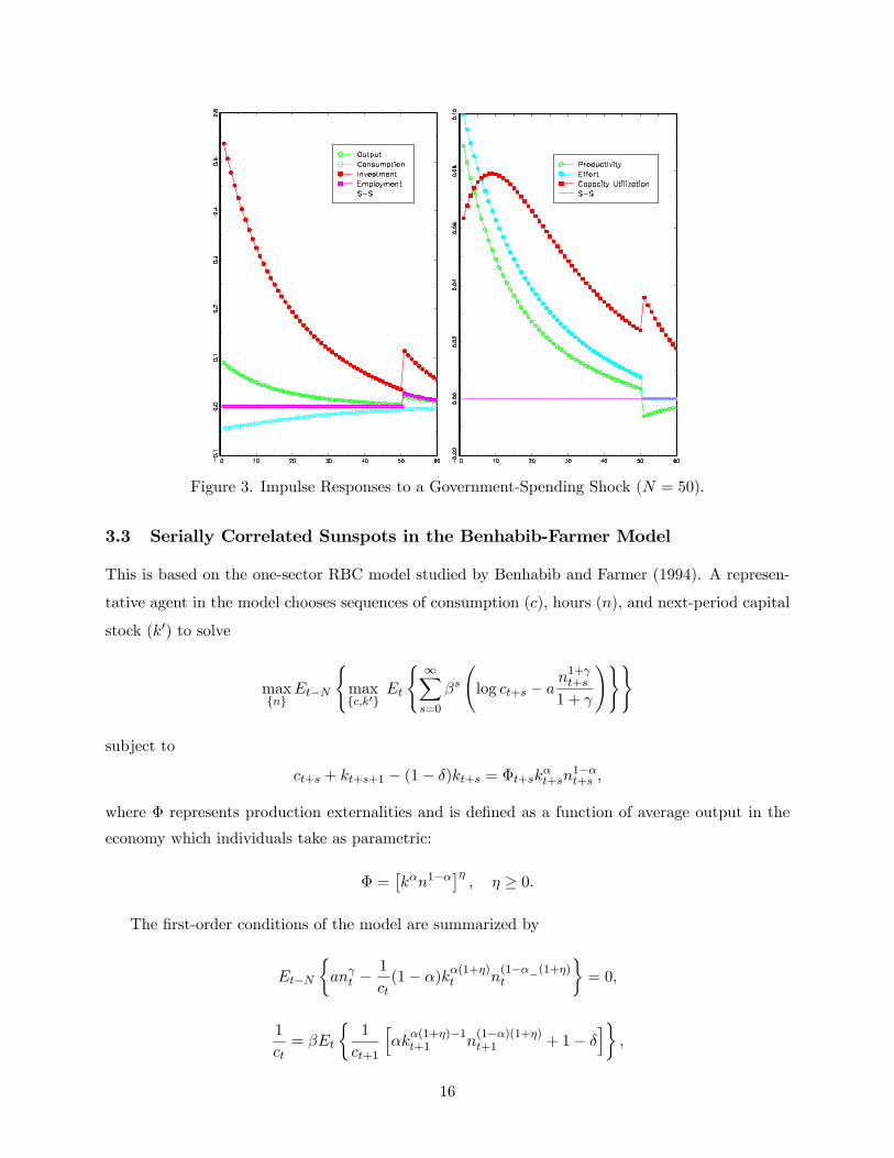
Figure 3. Impulse Responses to a Government-Spending Shock (N = 50).

3.3 Serially Correlated Sunspots in the Benhabib-Farmer Model

This is based on the one-sector RBC model studied by Benhabib and Farmer (1994). A represen-

tative agent in the model chooses sequences of consumption (c), hours (n), and next-period capital

stock (k0) to solve

maxfng

Et�N

(maxfc;k0g

Et

( 1Xs=0

�s

log ct+s � a

n1+ t+s

1 +

!))

subject to

ct+s + kt+s+1 � (1� �)kt+s = �t+sk�t+sn1��t+s ;

where � represents production externalities and is de�ned as a function of average output in the

economy which individuals take as parametric:

� =�k�n1��

��; � � 0:

The �rst-order conditions of the model are summarized by

Et�N

�an t �

1

ct(1� �)k�(1+�)t n

(1��_(1+�)t

�= 0;

1

ct= �Et

�1

ct+1

h�k

�(1+�)�1t+1 n

(1��)(1+�)t+1 + 1� �

i�;

16

ct + kt+1 � (1� �)kt = k�(1+�)t n(1��)(1+�)t :

Since labor is assumed to be determined N periods in advance as in the labor hoarding model, it

is known in period t. Thus the log-linearized �rst-order conditions of the model can be represented

by the following system of linear equations:

nt = AEt�NSt (25)

EtSt+1 +B1Et�NSt+1 = B2St +B3Et�NSt; (26)

where St = [kt; ct]0 denotes an expanded state vector and fA;B1; B2; B3g denote coe¢ cient ma-

trices. As discussed in Farmer (1999) for the case of N = 0, the model is indeterminate if � is

su¢ ciently large, hence it permits �uctuations driven by self-ful�lling expectations even in the ab-

sence of fundamental shocks. Farmer also shows that in the case of N = 0; the sunspots shocks to

expectations must be i:i:d: processes. To see this, let N = 0 and rearrange equation (26) (assuming

I +B1 is invertible) as

St+1 =MSt + C"t+1; (27)

where "t+1 = ct+1 �Etct+1 denotes the forecast errors that satisfy Et"t+1 = 0. In equilibrium, theeconomy can be subject to sunspots shocks if the matrix B has all of its eigenvalues lying inside the

unit circle. This will happen if and only if � is large enough. In this case, given the current state

of the economy (kt), any initial value of consumption (ct) can constitute an equilibrium. Hence

the forecast error does not need be related to fundamental shocks and can thus represent shocks to

agents�expectations.

Since �uctuations driven by self-ful�lling expectations in the Benhabib-Farmer model has to do

with the indeterminacy of the initial values of consumption or labor given the initial value of the

capital stock in each period, one may think naively that if at least one of these endogenous control

variables is predetermined, then indeterminacy can no longer arise in the model. This intuition is

false. For example, let labor be predetermined in this model by N > 0 periods in advance (the

same results hold if we let consumption be predetermined by N > 0 periods in advance). Let

St � Et�NSt =NXj=1

�j"t�j+1; �1 =

�01

�;�j = 0 for j � 0;

to represent the forecast errors of St. Equation (26) then becomes

(I +B1)EtSt+1 = (B2 +B3)St +B1 (EtSt+1 � Et�NSt+1)�B3 (St � Et�NSt)

= (B2 +B3)St +B1

NXj=1

�j+1"t�j+1 �B3NXj=1

�j"t�j+1;

17

which can be written as

EtSt+1 =MSt +NXj=1

Cj"t�j+1;

where Cj are 2 � N coe¢ cient matrices that depend on the undetermined coe¢ cients �i. Since

EtSt+1 = St+1 � �0"t+1; the above equation can be written as

St+1 =MSt +NXj=0

Cj"t�j+1; (28)

with C0 = �0. Notice that this representation reduces to the Benhabib-Famer model when N = 0.

It can be seen that the conditions for indeterminacy in this model are the same as those in the

Benhabib-Farmer model, since the matrix M is independent of N . Thus, if both of the eigenvalues

of M lie inside the unit circle due to a large enough value of the externality parameter �, any path

of consumption that satis�es

ct =M2St�1 +NXj=0

C2j"t�j+1 (29)

constitutes an equilibrium, where M2 and C2j are the second rows of the corresponding matrices.

The undetermined coe¢ cients f�jgNj=1 can be solved by the method proposed in the previous

section.

Impulse Responses. Following the existing literature, we calibrate the model by setting the

discount factor � = 0:99; the capital�s share � = 0:3; the inverse elasticity of labor supply = 0

(indivisible labor), and the rate of capital depreciation � = 0:025. The minimum degree of the

externality � required for indeterminacy under this parameterization is 0:49. We choose � = 0:75.

This value of � implies a degree of aggregate returns to scale at 1:75, which, based on recent

empirical studies is obviously too high.7 We set the variance of the sunspots shocks to �2" = 1

and the period of labor hoarding N = 10 quarters. The curves with solid circles in Figure 4 show

the impulse responses of output, consumption, investment, and employment to a one-standard-

deviation sunspots shock to consumption. Notice that in the initial N = 10 periods during which

labor is predetermined, the higher consumption level generated by the self-ful�lling expectations is

sustained by a lower level of savings (investment). This is optimal because the representative agent

anticipates high rates of of investment in the future by working harder later. This is also feasible

because of increasing returns to scale, which enables the agent to pay back any amount of debt in

savings by working harder 10 periods later. Thus, in the model, the longer that labor is hoarded7See Wen (1998) for a modi�ed model that can give rise to indeterminacy with nearly constant returns to scale

under very mild externalities. Also see Lubik and Schorfheide (2003, 2004) for how to test indeterminate DSGEmodels.

18

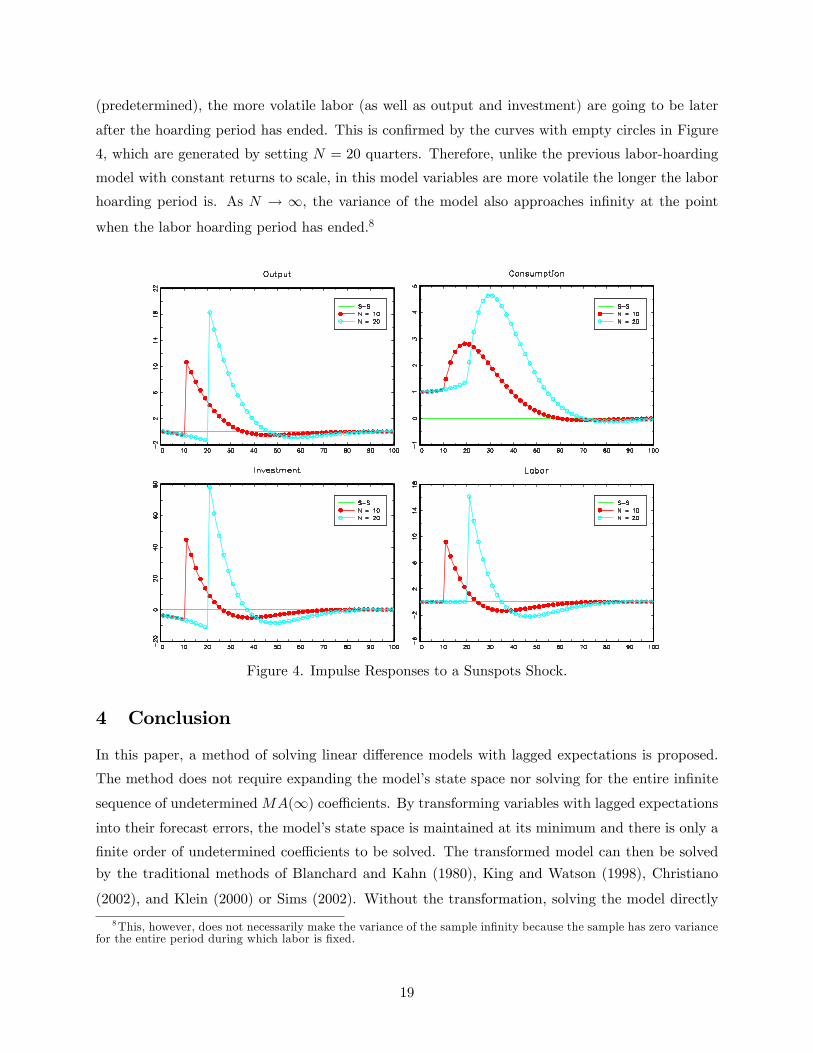
(predetermined), the more volatile labor (as well as output and investment) are going to be later

after the hoarding period has ended. This is con�rmed by the curves with empty circles in Figure

4, which are generated by setting N = 20 quarters. Therefore, unlike the previous labor-hoarding

model with constant returns to scale, in this model variables are more volatile the longer the labor

hoarding period is. As N ! 1, the variance of the model also approaches in�nity at the point

when the labor hoarding period has ended.8

Figure 4. Impulse Responses to a Sunspots Shock.

4 Conclusion

In this paper, a method of solving linear di¤erence models with lagged expectations is proposed.

The method does not require expanding the model�s state space nor solving for the entire in�nite

sequence of undeterminedMA(1) coe¢ cients. By transforming variables with lagged expectationsinto their forecast errors, the model�s state space is maintained at its minimum and there is only a

�nite order of undetermined coe¢ cients to be solved. The transformed model can then be solved

by the traditional methods of Blanchard and Kahn (1980), King and Watson (1998), Christiano

(2002), and Klein (2000) or Sims (2002). Without the transformation, solving the model directly

8This, however, does not necessarily make the variance of the sample in�nity because the sample has zero variancefor the entire period during which labor is �xed.

19

by the traditional methods can be very di¢ cult when the order of lagged expectations is large.

Several examples are provided in the paper to demonstrate the usefulness of our solution method.

These examples are also of independent interest to researchers in the business-cycle literature.

Appendix

This appendix outlines proofs for Proposition 1. Since equation (400) is a linear di¤erence

system in St with �t as the forcing variable, and since ~A and ~B are both independent of , the

solution of St must also be a linear function of the coe¢ cient of �t. In addition, this implies that

the endogenous dynamics of St in the absence of �t (i.e., the eigenvalues and eigenvectors of the

system) do not depend on . Hence the coe¢ cient matrices Hy and My in equations (7) and (8)

must be independent of , while H�() and M�() in equations (7) and (8) must be linear in .

Denote Yt = [Y 0; Z 0]0 ; G0 = [00; Im]

0 ; and rewrite equation (8) as

Yt =MyYt�1 +M��t�1 +G0"t:

Also rewrite equation (5) as

�t = ��t�1 + I0"t:

Based on these two equations, if we denote ejx = Et�jxt �Et�j�1xt as the one-step ahead forecasterror of variable Xt based on information j�1 periods ago, then we can compute the forecast errors

of Yt as

e0y

�= Yt � Et�1Yt

�= G0"t

e1y

�= Et�1Yt � Et�2Yt

�= [MyG0 +M�I0] "t�1

e2y

�= Et�2Yt � Et�3Yt

�= [My [MyG0 +M�I0] +M��I0] "t�2

...

ejy =�Mye

j�1y +M��

j�1I0�"t�j :

Notice the recursive nature of these one-step ahead forecast errors. Given that we can express

Yt =P1j=0�

yj "t�j , thus we have the relationships,

�y0 = G0

and

�yj =My�yj�1 +M�()�

j�1I0; for j � 1:

20

Also, based on equation (7), we have ejx = Hyejy +H�()�

jI0"t�j ; which implies

�xj = Hy�yj +H�()�

jI0:

Combining the above expressions for �yj and �xj , we can see that Pj() in equations (11) and (13)

is linear in for all j: Hence the undetermined coe¢ cients in St �Et�NSt =PN�1j=0 �j"t�j ; where

�j =h�xj ;�

yj

i0, can either be solved recursively in a linear fashion or be determined by solving

a simultaneous linear equation system composed of �j = Pj() for all j in terms of the linear

mapping, P () = .�

21

References

[1] Aadland, D., 2001, High-frequency real business cycle models, Journal of Monetary Economics

48 (2), 271�292.

[2] Aadland, D. and K.X.D. Huang, 2004, Consistent high-frequency calibration, Journal of Eco-

nomic Dynamics and Control 28(11), 2277-95.

[3] Andrés, J., D. López-Salido, and E. Nelson, 2005, Sticky-price models and the natural rate

hypothesis, Journal of Monetary Economics 52(5), 1025-53.

[4] Benhabib, J. and Farmer, R., 1994, Indeterminacy and increasing returns, Journal of Economic

Theory 63(1), 19-41.

[5] Blanchard, O. and C. Kahn, 1980, The solution of linear di¤erence models under rational

expectations, Econometrica 48(5), 1305-1312.

[6] Burnside, C. and Eichenbaum, M., 1996, Factor-hoarding and the propagation of business-cycle

shocks, American Economic Review 86(5), 1154-1174.

[7] Burnside, C., Eichenbaum, M. and Rebelo, S., 1993, Labor hoarding and the business cycle,

Journal of Political Economy 101(2), 245-273.

[8] Christiano, L., 2002, Solving dynamic equilibrium models by a method of undetermined coef-

�cients, Computational Economics 20, 21-55.

[9] Christiano, L., M. Eichenbaum, and C. Evans, 2005, Nominal rigidities and the dynamic e¤ects

of a shock to monetary policy, Journal of Political Economy 113(1), 1-45.

[10] Farmer, R., 1999, Macroeconomics of Self-ful�lling Prophecies, Second Edition, The MIT

Press.

[11] Fuhrer, J. and G. Moore, 1995, In�ation persistence, The Quarterly Journal of Economics

110(1), 127-59.

[12] Klein, P., 2000, Using the generalized Schur form to solve a multivariate linear rational expec-

tations model, Journal of Economic Dynamics and Control 24(10), 1405-23.

[13] Keen, B., 2004, Sticky price and sticky information price setting models: What is the di¤er-

ence?, Working Paper, Department of Economics, University of Oklahoma.

22

[14] King, R.G. and M. Watson, 1998, The solution of singular linear di¤erence systems under

rational expectations, International Economic Review 39(4), 1015-1026.

[15] Lubik, T. and F. Schorfheide, 2003, Computing sunspot equilibria in linear rational expecta-

tions models, Journal of Economic Dynamics and Control 28(2), 273-285.

[16] Lubik, T. and F. Schorfheide, 2004, Testing for indeterminacy: An application to U.S. mone-

tary policy, American Economic Review 94(1), 190-217.

[17] Mankiw, N.G. and R. Reis, 2002, Sticky information versus sticky prices: A proposal to replace

the New Keynesian Phillips Curve, Quarterly Journal of Economics 117(4), 1295-1328.

[18] Sims, C., 2002, Solving linear rational expectations models, Computational Economics 20,

1-20.

[19] Taylor, J., 1986, New econometric approaches to stabilization policy in stochastic models of

macroeconomic �uctuations, in Handbook of Econometrics, Vol. 3, Zvi Griliches and M. D.

Intriligator, eds., North Holland, 1997-2055.

[20] Trabandt, M., 2005, Sticky information vs. sticky prices: A horse race in a DSGE framework,

Working Paper, Humboldt University Berlin.

[21] Wang, P.F. and Y. Wen, 2005, In�ation and money: A puzzle, Working Paper 2005-076A,

Federal Reserve Bank of St. Louis.

[22] Wen, Y., 1998, Capacity utilization under increasing returns to scale, Journal of Economic

Theory 81(1), 7-36.

23