solving a multi-stage multi-product solid supply chain...

Scientia Iranica E (2016) 23(3), 1429{1440

Sharif University of TechnologyScientia Iranica

Transactions E: Industrial Engineeringwww.scientiairanica.com

Solving a multi-stage multi-product solid supply chainnetwork design problem by meta-heuristics

A. Mahmoodirad� and M. Sanei

Department of Mathematics, Central Tehran Branch, Islamic Azad University, Tehran, Iran.

Received 6 October 2014; received in revised form 10 May 2015; accepted 16 June 2015

KEYWORDSSupply chain networkdesign;Di�erential evolution;Particle swarmoptimizationalgorithm;Gravitational searchalgorithm;Taguchi experimentalDesign.

Abstract. This paper presents an e�ective optimization method based on meta-heuristicsalgorithms for the design of a multi-stage, multi-product solid supply chain network designproblem. First, a mixed integer linear programming model is proposed. Second, becausethe problem is an NP-hard, three meta-heuristics algorithms, namely Di�erential Evolution(DE), Particle Swarm Optimization (PSO), and Gravitational Search Algorithm (GSA),are developed for the �rst time for this kind of problem. To the best of our knowledge,neither DE, nor PSO, nor GSA have been considered for the multi-stage solid supply chainnetwork design problems. Furthermore, the Taguchi experimental design method is usedto adjust the parameters and operators of the proposed algorithms. Finally, to evaluatethe impact of increasing the problem size on the performance of our proposed algorithms,di�erent problem sizes are applied and the associated results are compared with each other.© 2016 Sharif University of Technology. All rights reserved.

1. Introduction

The Supply Chain Network (SCN) design problemis an important strategic issue in supply chain man-agement that has recently drawn the focus of manyresearchers [1-4].

SCN is widely used and includes all activities inthe �eld of production and the �nal product providesthe service of distribution of the most elementary stage,i.e. from the primary stage of raw materials, to themost �nal stage, i.e. delivery to the customer and evenworn out product recycling. Supply chain manage-ment includes managing supply and demand, supplyof components and raw materials, manufacturing andassembly, storage and shipping of inventory, ordermanagement, distribution channels, and supply anddelivery to the customer. Nowadays, service providers

*. Corresponding author. Tel.: +98 21 66434096;Fax: +98 21 66434099E-mail addresses: [email protected] (A.Mahmoodirad); [email protected] (M. Sanei)

and products, distribution channels (distributors andwholesalers), and customers as well as supply chainmanagement consultants, system developers and sup-pliers of software products, and supply chain managersare all key elements. Achieving the e�ective supplychain management is dependent on the cooperation ofsupply chain members.

A Multi-stage Supply Chain Network (MSCN)can be modeled by means of a sequence of multipleSCN stages for production of multi-product so that the ow would be transferred only between two successivestages. Since the MSCN is di�cult to solve opti-mally [5], many researchers have developed heuristicand meta-heuristic approaches to solve it. The workdone in this regard is as follows.

Jayaraman and Pirkul [6] have presented ane�cient heuristic approach based on the Lagrangeanrelaxation for the single-source, multi-product, multi-stage SCN design problem. They use this heuristicmethod to evaluate the performance of the model withrespect to solution quality and algorithm performance.Syam [7] focused on a heuristic method proposed based

1430 A. Mahmoodirad and M. Sanei/Scientia Iranica, Transactions E: Industrial Engineering 23 (2016) 1429{1440

on Lagrangean relaxation and simulated annealing fora multi-source, multi-product, multi-location frame-work. Another heuristic approach based on steady-state genetic algorithm has been developed by Alti-parmak et al. [5] for a single-source, multi-product,multi-stage SCN design problem. They propose twodi�erent encoding approaches to represent a solutionto the problems: priority-based encoding and integerencoding. The priority-based encoding is used forthe �rst two stages of SCN and integer encoding isused in the last stage. Moreover, the e�ciency ande�ectiveness of the algorithm have been investigatedby comparing its results with those of other methodssuch as CPLEX, Lagrangean heuristic, hybrid geneticalgorithm, and simulated annealing on a set of SCNdesign problems with di�erent sizes.

Mehdizadeh and Afrabandpei [8] have proposeda mixed integer nonlinear programming model for themulti-stage, multi-product network design problem tominimize the total cost of supply chain. They havedeveloped a hybrid priority-based Genetic Algorithm(GA) and simulated annealing algorithm to �nd op-timal solution in two phases. In the �rst phase,the optimal routes are determined by the use of GA.In the second phase, they use the SA algorithm forconvergence speed. They use a matrix and vectorto represent the solution. The obtained results haveshown that the proposed algorithms can �nd nearoptimal solutions in reasonable time spans.

Kadadevaramath et al. [9] have presented aninteger linear programming model for the constrainedthree echelons SCN problem to minimize the totalsupply chain operating cost. They have used fouralgorithms based on a Particle Swarm Optimization(PSO) algorithm and Genetic Algorithm (GA) forsolving the problem and the obtained results of PSOalgorithms have been compared with those of GA.

Olivares-Benitez et al. [10] addressed a supplychain design problem based on a two-echelon single-product system. The meta-heuristic algorithm was pro-posed to solve the problem, which combined principlesof greedy functions, Scatter search, Path relinking, andMathematical programming.

Mehdizadeh et al. [3] considered an integratedmulti-stage, multi-product logistic network designproblem which included forward and reverse logisticsand proposed a mixed integer nonlinear programmingmodel. To �nd the proper solutions, they developedtwo meta-heuristic algorithms, namely hybrid priority-based genetic algorithm and simulated annealing al-gorithm. In order to tune the signi�cant parametersof the algorithms, they used the response surfacemethodology.

Crdenas-Barron and Trevino-Garza [11] devel-oped a more general mathematical model proposed byKadadevaramath et al. [9] when the number of periods

and products was one. They solved all instances inKadadevaramath et al. [9] by CPLEX and showed thatall instances could easily be solved optimally by anyinteger linear programming solver.

Kristianto et al. [12] developed a supply chainnetwork by optimizing inventory allocation and trans-portation routing. They proposed a fuzzy shortest pathinto two-stage programming in order to �nd the globaloptimum solution.

Khalifehzadeh et al. [13] considered a four-echelonsupply chain network design with shortage. Theypresented a multi-objective mathematical model tominimize the total operating costs of all the supplychain elements and to maximize reliability of thesystem. They solved this problem by a comparativeparticle swarm optimization algorithm.

The multi-product, multi-stage solid SCN designproblem considered in this paper consists of threestages: supplier, plant, DC and customer. The problemis to determine the optimal transportation networkin order to satisfy the customer demands of productsby using several kinds of conveyance with minimumcosts. To this end, �rstly, we propose a mixed integerprogramming model for the multi-product, multi-stagesolid SCN design problem, in which the objectiveis minimization of the total costs of supply chain.Secondly, due to complexity of the problem, we developthree meta-heuristic algorithms, namely Di�erentialEvolution (DE), Particle Swarm Optimization (PSO),and Gravitational Search Algorithm (GSA), for thisproblem. Furthermore, the Taguchi experimentaldesign method is used to adjust the parameters andoperators of the proposed algorithms. Finally, toevaluate the impact of increasing the problem size onthe performance of our proposed algorithms, di�erentproblem sizes are applied and the associated results arecompared with each other.

The rest of this paper is arranged as follows:In Section 2, we describe the mathematical modeland descriptions. Section 3 explains the proposedsolution approaches. Section 4 describes the Taguchiexperimental design and compares the computationalresults. Finally, in Section 5, conclusions are made andprovided.

2. Problem description and mathematicalmodel

The considered problem can formally be described asfollows:

The multi-stage, multi-product solid SCN designproblem can consist of suppliers, plants, DCs, andcustomers. In the �rst stage, the suppliers providethe raw materials for the plants to produce multi-product. In the second stage, the plants produce andsend the products to DCs. Finally, the DCs transport

A. Mahmoodirad and M. Sanei/Scientia Iranica, Transactions E: Industrial Engineering 23 (2016) 1429{1440 1431

the products to the customers. Also, conveyances canbe considered as transportation types so that eachconveyance would be related to the cost, and one mustbe selected to transport the products to each stage.The objective is minimization of the total costs ofsupply chain that will satisfy all capacities and demandrequirement for each product imposed by customers.We formulated this problem as a mixed-integer non-linear programming model. The assumption used inthis problem is as follows:

� The number of suppliers, the maximum numberof plants, the maximum number of DCs, and thenumber of conveyances are known;

� The capacities of suppliers, plants, and DCs areknown;

� The number of customers and their demands areknown.

The following notations are used to de�ne the mathe-matical model:

Set of indices:R Set of raw materials (r = 1; 2; � � � ; R);P Set of products (p = 1; 2; � � � ; P );S Set of suppliers (s = 1; 2; � � � ; S);I Set of plants (i = 1; 2; � � � ; I);J Set of DCs (j = 1; 2; � � � ; J);K Set of customers (k = 1; 2; � � � ;K);M Set of conveyances in the �rst stage

(m = 1; 2; � � � ;M);N Set of conveyances in the second stage

(n = 1; 2; � � � ; N);L Set of conveyances in the third stage

(l = 1; 2; � � � ; L).Parameters:Esr Capacity of supplier s for raw

material r;Di Capacity of plant i;Wj Capacity of DCj;Cpk Demand for product p at customer k;urp Utilization rate of raw material r per

unit of product p;Fi Fixed cost for operating a plant i;Gj Fixed cost for operating a DCj;arsim Cost of transporting and purchasing

for raw material r from supplier s toplant i by conveyance m;

bpijn Cost of transporting one unit ofproduct p from plant i to DCj byconveyance n;

cpjkl Cost of sending one unit of product pfrom DCj to customer k by conveyancel;

fsim Fixed cost of transporting for rawmaterials from supplier s to plant i byconveyance m;

gijn Fixed cost of transporting productsfrom plant i to DCj by conveyance n;

hjkl Fixed cost of sending products fromDCj to customer k by conveyance l;

vi Unit production cost of product atplant i;

v0j Unit storing cost of product at DCj;

E(1)m Maximum capacity of conveyance m in

the �rst stage;

E(2)n Maximum capacity of conveyance n in

the second stage;

E(3)l Maximum capacity of conveyance l in

the third stage.Decision variables:�i Binary variable equal to 1 if plant i is

opened and equal to 0 otherwise;�j Binary variable equal to 1 if DCj is

opened and equal to 0 otherwise;xrsim Quantity of raw material r shipped

from supplier s to plant i byconveyance m;

ypijn Quantity of product p shipped fromplant i to DCj by conveyance n;

zpjkl Quantity of product p shipped fromDCj to customer k by conveyance l;

t(1)sim Binary variable equal to 1 ifPR

r=1 xrsim > 0 and equal to 0otherwise;

t(2)ijn Binary variable equal to 1 ifPP

p=1 ypijn > 0 and equal to 0otherwise;

t(3)jkl Binary variable equal to 1 ifPP

p=1 zpjkl > 0 and equal to 0otherwise.

The mathematical model of the multi-stage, multi-product solid SCN design problem is as follows:

MinZ =RXr=1

SXs=1

IXi=1

MXm=1

arsimxrsim

+PXp=1

IXi=1

JXj=1

NXn=1

bpijnypijn


+PXp=1

JXj=1

KXk=1

LXl=1

cpjklzpjkl

+SXs=1

IXi=1

MXm=1

fsimt(1)sim +

IXi=1

JXj=1

NXn=1

gijnt(2)ijn

+JXj=1

KXk=1

LXl=1

hjklt(3)jkl +

IXi=1

Fi�i +JXj=1

Gj�j

+PXp=1

IXi=1

JXj=1

NXn=1

viypijn

+PXp=1

IXi=1

JXj=1

NXn=1

v0jypijn; (1)

subject to:IXi=1

MXm=1

xrsim � Esr 8s; r; (2)

PXp=1

JXj=1

NXn=1

ypijn � Di�i 8i; (3)

PXp=1

JXj=1

NXn=1

urpypijn �SXs=1

MXm=1

xrsim 8r; i; (4)

PXp=1

IXi=1

NXn=1

ypijn �Wj�j 8j; (5)

KXk=1

LXl=1

zpjkl �IXi=1

NXn=1

ypijn 8j; p; (6)

JXj=1

LXl=1

zpjkl � Cpk 8p; k; (7)

RXr=1

SXs=1

IXi=1

xrsim � E(1)m 8m; (8)

PXp=1

IXi=1

JXj=1

ypijn � E(2)n 8n; (9)

PXp=1

JXj=1

KXk=1

zpjkl � E(3)l 8l; (10)

�i 2 f0; 1g 8i; (11)

�j 2 f0; 1g 8j; (12)

t(1)sim 2 f0; 1g 8s; i;m; (13)

t(2)ijn 2 f0; 1g 8i; j; n; (14)

t(3)jkl 2 f0; 1g 8j; k; l; (15)

xrsim; ypijn; zpjkl � 0 8r; p; s; i; j; k;m; n; l: (16)

In this model, objective function (1) minimizes thetotal cost of supply chain network. Constraint (2) is thecapacity constraint for the suppliers. Constraint (3)gives the plant capacity constraint. Constraint (4)gives the raw material requirement. Constraint (5) isthe capacity constraint for DCs. Constraint (6) limitsthe total quantity of products shipped from a DC tocustomers and cannot exceed the amount of shippedproducts in that DC. Constraint (7) represents demandsatisfaction for each customer. Constraints (8)-(10)give capacity constraint for conveyance in the �rst,second, and third stages, respectively. Ultimately,Constraint sets (11)-(16) de�ne the decision variables.

Since the problem is minimization of the objectivefunction, in the optimal solution, no extra productsor raw materials are transported at various stagesof the supply chain network. Thus, in the optimalsolution of the equality, Constraints (4), (6), and (7)are established.

3. Solution approach

Although the exact algorithms such as DynamicProgramming, local search techniques, Branch-and-Cut, Branch-and-Bound, Branch-and-Price, and La-grangean relaxation guarantee the optimal solution orprove that no feasible solution exists, the real-worldproblems are time consuming. Therefore, the meta-heuristic algorithms to �nd the near optimal solutionin a reasonable time have been proposed by researchers.The meta-heuristics are simple, easy to implement,robust, and have proven to be highly e�ective to solvemany optimization problems [14].

Since the single-stage �xed cost transportationproblem can be categorized as NP-hard [15,16], themulti-stage, multi-product solid SCN design problemis NP-hard, too. In this section, �rst, the solution rep-resentation is described and then three meta-heuristicalgorithms are developed to �nd the near optimalsolutions.

3.1. Encoding scheme and initializationThe encoding scheme plays a very important role in thee�ectiveness of the meta-heuristic algorithms. In fact,it is the approach of making a solution recognizablefor the meta-heuristic algorithms. Among di�erentmethods of encoding, the priority-based encoding hassuccessfully been applied for many optimization prob-lems [3,5,17-19]. It needs no repairing process and itbelongs to the permutation encoding category [19].


In the single-stage �xed cost solid transportationproblem, we have two three-dimensional cost matrices,namely the three-dimensional variable cost matrix andthe three-dimensional �xed cost matrix. Therefore,selecting a route with minimum variable cost will notgive good solutions.

When the priority-based encoding is utilized forthe single-stage, single-product �xed cost solid trans-portation problem, a solution consists of priorities ofsources (M), depots (N), and conveyances (K); inthis case, the solution length is equal to jQj = jM j +jN j+ jKj. In the single-stage, multi-product �xed costsolid transportation problem, consider P to be the setof products. In this case, the solution based on thepriority-based encoding consists of jP j parts and the

length of each part is equal to jP j � jQj, and the digitvalues of the solution are between 1 and jP j � jQj. Toobtain the priority-based encoding, in the single-stage,multi-product �xed cost solid transportation problem,a priority assignment to nodes is started from thehighest value (jP j � jQj) and it is reduced by one untilassigning a priority to all nodes.

In this paper, we develop the priority-based de-coding procedure developed by Gen et al. [17,20] andAltiparmak et al. [5] to adapt to the single-stage, multi-product �xed cost solid transportation problem. Theprocedure to decode the solution of the single-stage,multi-product �xed cost solid transportation problemis shown in Figure 1.

In the multi-stage, multi-product solid SCN prob-

Figure 1. Priority-based decoding procedure for the SFCSTP.


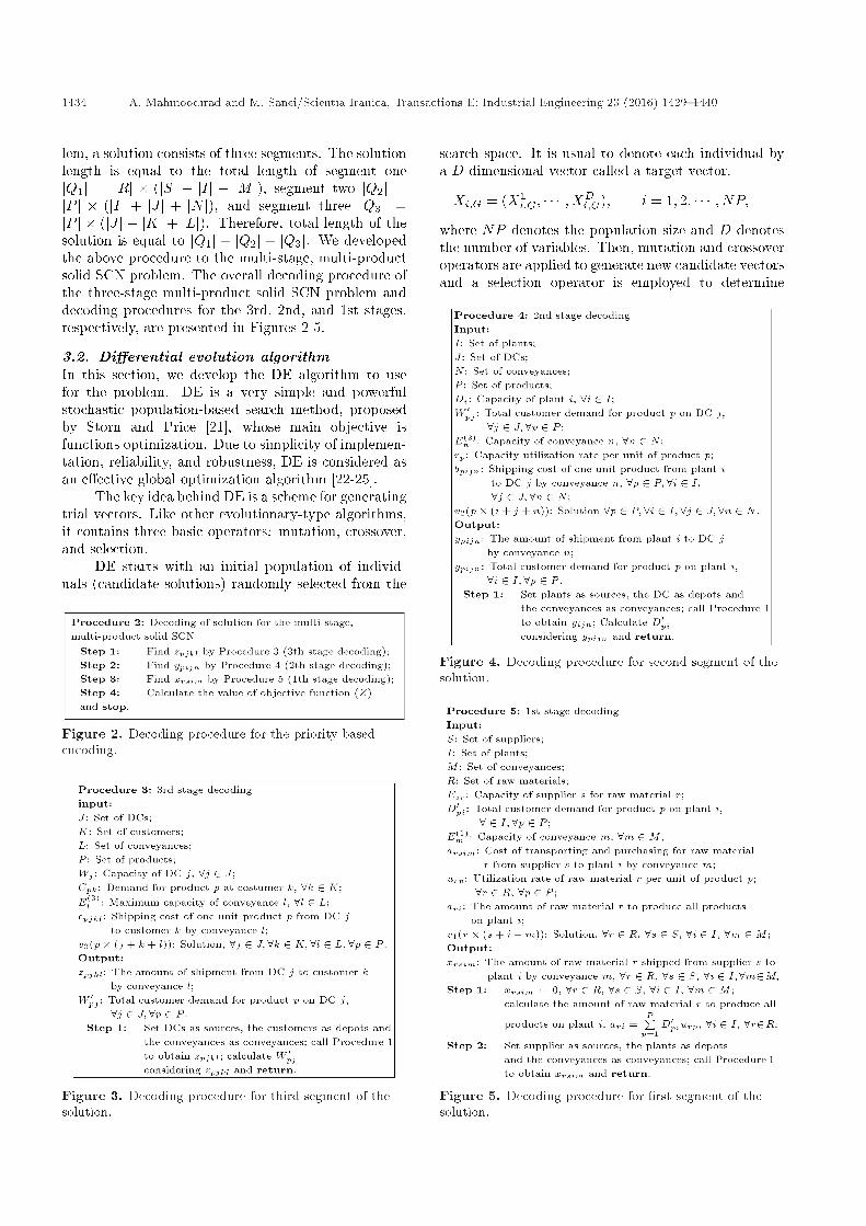
lem, a solution consists of three segments. The solutionlength is equal to the total length of segment onejQ1j = jRj � (jSj + jIj + jM j), segment two jQ2j =jP j � (jIj + jJ j + jN j), and segment three jQ3j =jP j � (jJ j + jKj + jLj). Therefore, total length of thesolution is equal to jQ1j + jQ2j + jQ3j. We developedthe above procedure to the multi-stage, multi-productsolid SCN problem. The overall decoding procedure ofthe three-stage multi-product solid SCN problem anddecoding procedures for the 3rd, 2nd, and 1st stages,respectively, are presented in Figures 2-5.

3.2. Di�erential evolution algorithmIn this section, we develop the DE algorithm to usefor the problem. DE is a very simple and powerfulstochastic population-based search method, proposedby Storn and Price [21], whose main objective isfunctions optimization. Due to simplicity of implemen-tation, reliability, and robustness, DE is considered asan e�ective global optimization algorithm [22-25].

The key idea behind DE is a scheme for generatingtrial vectors. Like other evolutionary-type algorithms,it contains three basic operators: mutation, crossover,and selection.

DE starts with an initial population of individ-uals (candidate solutions) randomly selected from the

Figure 2. Decoding procedure for the priority basedencoding.

Figure 3. Decoding procedure for third segment of thesolution.

search space. It is usual to denote each individual bya D-dimensional vector called a target vector.

Xi;G = (X1i;G; � � � ; XD

i;G); i = 1; 2; � � � ; NP;where NP denotes the population size and D denotesthe number of variables. Then, mutation and crossoveroperators are applied to generate new candidate vectorsand a selection operator is employed to determine

Figure 4. Decoding procedure for second segment of thesolution.

Figure 5. Decoding procedure for �rst segment of thesolution.


whether the o�spring or the parent survives in thenext generation. The above process is repeated untila termination criterion is reached. According to Stornand Price [21], the strategy of DE is described below.

3.2.1. Mutation operatorFor each target vectorXi;G, i = 1; 2; � � � ; NP , a mutantvector Vi;G is generated according to the followingscheme:

Vi;G = Xr1;G + F (Xr2;G �Xr3;G);

r1 6= r2 6= r3 6= i;

with randomly chosen indices and r1; r2; r3 2 f1; 2; � � � ;NPg. Note that these indices have to be di�erentfrom each other and from the running index i so thatNP must be at least 4. According to Storn andPrice [21], F 2 [0; 2] is to control the ampli�cationof the di�erence vector.

3.2.2. Crossover operatorIn order to increase diversity of the perturbed parame-ter vectors, crossover is introduced after the mutationoperation. The target vector is mixed with the mutatedvector to get the trial vector Ui;G+1 according to thefollowing [21]:

Ui;j;G+1 =

8>>><>>>:Vi;j;G+1 if rand(j) � CR or

j = rand(i)Xi;j;G+1 if rand(j) > CR or

j 6= rand(i)

where rand(j) is the jth evaluation of a randomnumber uniformly distributed in the range [0; 1] andrandn(i) is a randomly chosen index from the setf1; 2; � � � ; Ng. CR 2 [0; 1] is a crossover constant ratethat controls the diversity of the population. The morethe value of CR, the less the in uence of the parent willbe.

3.2.3. Selection operatorTo generate better o�spring for the next generation,selection operation is performed between each individ-ual and its corresponding trial vector by the followinggreedy selection criterion:

Xi;G+1 =

(Ui;G+1 if f(Ui;G+1) < f(Xi;G);Xi;G otherwise;

where f is the objective function and Xi;G+1 is theindividual of the new population.

The steps of DE are shown in Figure 6.

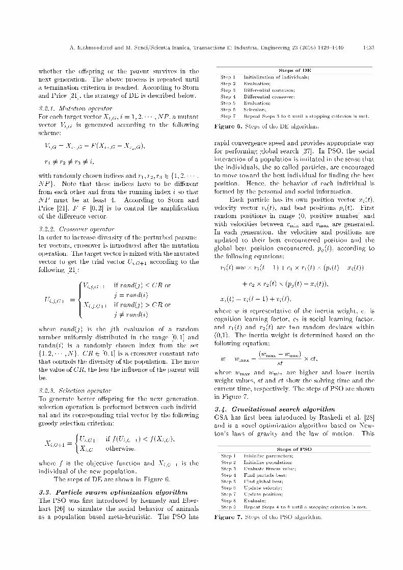
3.3. Particle swarm optimization algorithmThe PSO was �rst introduced by Kennedy and Eber-hart [26] to simulate the social behavior of animalsas a population based meta-heuristic. The PSO has

Figure 6. Steps of the DE algorithm.

rapid convergence speed and provides appropriate wayfor performing global search [27]. In PSO, the socialinteraction of a population is imitated in the sense thatthe individuals, the so called particles, are encouragedto move toward the best individual for �nding the bestposition. Hence, the behavior of each individual isformed by the personal and social information.

Each particle has its own position vector xi(t),velocity vector vi(t), and best positions pi(t). Firstrandom positions in range (0, positive number] andwith velocities between vmin and vmax are generated.In each generation, the velocities and positions areupdated to their best encountered position and theglobal best position encountered, pg(t), according tothe following equations:

vi(t) =w � vi(t� 1) + c1 � r1(t)� (pi(t)� xi(t))+ c2 � r2(t)� (pg(t)� xi(t));

xi(t) = vi(t� 1) + vi(t);

where w is representative of the inertia weight, c1 iscognition learning factor, c2 is social learning factor,and r1(t) and r2(t) are two random deviates within(0,1). The inertia weight is determined based on thefollowing equation:

w = wmax � (wmax � wmin)st

� ct;where wmax and wmin are higher and lower inertiaweight values, st and ct show the solving time and thecurrent time, respectively. The steps of PSO are shownin Figure 7.

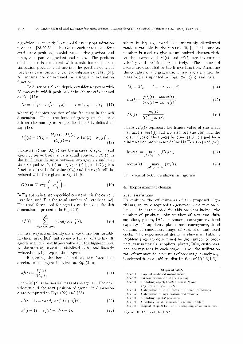
3.4. Gravitational search algorithmGSA has �rst been introduced by Rashedi et al. [28]and is a novel optimization algorithm based on New-ton's laws of gravity and the law of motion. This

Figure 7. Steps of the PSO algorithm.


algorithm has recently been used for many optimizationproblems [23,29,30]. In GSA, each mass has fourattributes: position, inertial mass, active gravitationalmass, and passive gravitational mass. The positionof the mass is consistent with a solution of the op-timization problem and moving the position of agentresults in an improvement of the solution's quality [31].All masses are determined by using the evaluationfunction.

To describe GSA in depth, consider a system withN masses in which position of the ith mass is de�nedas Eq. (17):

Xi = (x1i ; � � � ; xdi ; � � � ; xni ) i = 1; 2; � � � ; N; (17)

where xdi denotes position of the ith mass in the dthdimension. Then, the force of gravity on the massi from the mass j at a speci�c time t is de�ned asEq. (18):

F dij(t) = G(t)� Mi(t)�Mj(t)Rij(t) + E � �xdj (t)� xdi (t)� ;

(18)

where Mi(t) and Mj(t) are the masses of agent i andagent j, respectively, E is a small constant, Rij(t) isthe Euclidean distance between two agents i and j attime t equal to Rij(t) = jjxi(t); xj(t)jj2, and G(t) is afunction of the initial value (G0) and time t; it will bereduced with time given in Eq. (19):

G(t) = G0 exp�� t

T

�: (19)

In Eq. (3), � is a user-speci�ed constant, t is the currentiteration, and T is the total number of iterations [32].The total force used for agent i at time t in the dthdimension is presented in Eq. (20):

F di (t) =NX

j2Kbest;j 6=irandj � F dij(t); (20)

where randj is a uniformly distributed random variablein the interval [0,1] and Kbest is the set of the �rst Kagents with the best �tness value and the biggest mass.At the starting, Kbest is initialized at K0 and linearlyreduced step-by-step as time lapses.

Regarding the law of motion, the force thataccelerates the agent i is given as Eq. (21):

adi (t) =F di (t)Mii(t)

; (21)

whereMi(t) is the inertial mass of the agent i. The nextvelocity and the next position of agent i in dimensiond are computed in Eqs. (22) and (23):

vdi (t+ 1) = randi � vdi (t) + adi (t); (22)

xdi (t+ 1) = xdi (t) + vdi (t+ 1); (23)

where in Eq. (6), randi is a uniformly distributedrandom variable in the interval [0,1]. This randomnumber is used to give a randomized characteristicto the search and vdi (t) and xdi (t) are its currentvelocity and position, respectively. The masses ofagents are evaluated by the �tness function. Assumingthe equality of the gravitational and inertia mass, themass Mi(t) is updated by Eqs. (24), (25), and (26):

Mi = Mii i = 1; 2; � � � ; N; (24)

mi(t) =fiti(t)� worst(t)best(t)� worst(t) ; (25)

Mi(t) =mi(t)PNj=1mj(t)

; (26)

where fiti(t) represent the �tness value of the agenti at time t, best(t) and worst(t) are the best and theworst values of the �tness function at time t and for aminimization problem are de�ned in Eqs. (27) and (28).

best(t) = minj21;2;�� ;N fitj(t); (27)

worst(t) = maxj21;2;�� ;N fitj(t): (28)

The steps of GSA are shown in Figure 8.

4. Experimental design

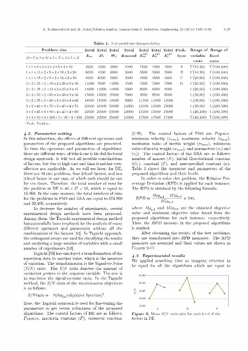
4.1. InstancesTo evaluate the e�ectiveness of the proposed algo-rithms, we were required to generate some test prob-lems. The data needed for this problem include thenumber of products, the number of raw materials,suppliers, plants, DCs, customers, conveyances, totalcapacity of suppliers, plants and conveyance, totaldemand of customers, range of variables, and �xedcosts. The experimental design is shown in Table 1.Problem sizes are determined by the number of prod-ucts, raw materials, suppliers, plants, DCs, customers,and conveyances in each stage. Also, the utilizationrate of raw material r per unit of product p, namely urp,is selected from a uniform distribution of U(0:5; 1:5).

Figure 8. Steps of the GSA.


Table 1. Test problems characteristics.

Problem size TotalEsr

TotalDi

TotalWj

Totaldemand

TotalE(1)m

TotalE(2)n

TotalE(3)l

Prob.�

typeRange of Range of

R�P�S�M�I�N�J�L�K variablecosts

�xedcosts

1�1�5�2�3�2�5�2�10 3000 2000 3000 1000 1500 1500 1500 A U(10,30) U(100,500)1�1�10�2�5�2�10�2�20 6000 4000 6000 2000 3000 3000 3000 B U(10,30) U(100,500)1�1�15�2�8�2�15�2�30 8000 6000 8000 3000 4500 4500 4500 C U(20,50) U(100,500)2�2�20�2�10�2�20�3�40 11000 9000 11000 4500 7000 7000 7000 D U(20,50) U(100,500)2�2�25�2�15�3�25�3�45 14000 12000 14000 5000 8000 8000 8000 U(20,50) U(100,500)2�2�30�2�50�3�30�3�50 15000 13000 15000 7000 9500 9500 9500 U(30,60) U(100,500)3�2�35�3�60�3�35�4�60 18000 15000 18000 9000 11000 11000 11000 U(30,60) U(100,500)3�2�40�3�70�3�45�4�75 20000 18000 20000 11000 13000 13000 13000 U(30,80) U(100,500)3�2�45�3�80�4�45�4�80 22000 20000 22000 13000 15000 15000 15000 U(40,100) U(100,500)3�3�50�3�100�5�50�4�100 25000 23000 25000 15000 17500 17500 17500 U(40,100) U(100,500)�Prob: Problem

4.2. Parameter settingIn this subsection, the e�ects of di�erent operators andparameters of the proposed algorithms are presented.To tune the operators and parameters of algorithms,there are di�erent ways, of which one is the full factorialdesign approach. It will test all possible combinationsof factors, but due to high cost and time is neither cost-e�ective nor applicable. As we will see later, for DE,there are 40 test problems, four 3-level factors, and one3-level factor in our case, of which each should be runfor ten times. Therefore, the total number of runs forthe problem in DE is 40 � 33 � 10, which is equal to10,800. In the same manner, the total numbers of runsfor the problems in PSO and GSA are equal to 874,800and 32,400, respectively.

To decrease the number of experiments, severalexperimental design methods have been proposed.Among them, the Taguchi experimental design methodhas successfully been employed for the analysis of manydi�erent operators and parameters without all thecombinations of the factors [33]. In Taguchi approach,the orthogonal arrays are used for classifying the resultsand analyzing a large number of variables with a smallnumber of experiments [16].

Taguchi [33] has employed a transformation of therepetition data to another value, which is the measureof variation. The transformation is the Signal-to-Noise(S=N) ratio. The S=N ratio denotes the amount ofvariations present in the response variable. The aim isto maximize the signal-to-noise ratio. In the Taguchimethod, the S=N ratio of the maximization objectivesis as follows:

S=Nratio = �10 log10(objective function)2:

Here, the Taguchi approach is used for �ne-tuning theparameters to get better robustness of the proposedalgorithms. The control factors of DE are as follows:Popsize, mutation constant (F ), crossover constant

(CR). The control factors of PSO are Popsize,minimum velocity (vmin), maximum velocity (vmax),maximum value of inertia weight (wmax), minimumvalue of inertia weight (wmin), and parameters (c1) and(c2). The control factors of the GSA are as follows:number of masses (N), initial Gravitational constant(G0), constant (E), and user-speci�ed constant (�).Table 2 shows the operators and parameters of theproposed algorithms and their levels.

In order to solve this problem, the Relative Per-centage Deviation (RPD) is applied for each instance.The RPD is obtained by the following formula:

RPD =Alogsol �Minsol

Minsol� 100;

where Algsol and Minsol are the obtained objectivevalue and minimum objective value found from theproposed algorithms for each instance, respectively.Thus, the RPD measure in the proposed algorithmsis applied.

After obtaining the results of the test problems,they are transformed into RPD measures. The RPDmeasures are averaged and their values are shown inFigures 9-11.

4.3. Experimental resultsWe applied searching time as stopping criterion tobe equal for all the algorithms which are equal to

Figure 9. Mean S=N ratio plot for each level of thefactors in DE.


Table 2. Factors and their levels.

DE factors DE levels PSO factors PSO levels GSA factors GSA levels

Popsize A(1)-80 Popsize A(1)-50 N A(1)-50

A(2)-90 A(2)-55 A(2)-60

A(3)-95 A(3)-60 A(3)-70

F B(1)-0.45 vmin B(1)- (-2) G0 B(1)-40

B(2)-1 B(2)- (-1.5) B(2)-60

B(3)-1.5 B(3)- (-1) B(3)-80

CR C(1)-0.3 vmax C(1)-2.5 E C(1)-0.005

C(2)-0.4 C(2)-3 C(2)-0.007

C(3)-0.5 C(3)-3.5 C(3)-0.009

c1 D(1)-0.3 � D(1)-7

D(2)-0.4 D(2)-12

D(3)-0.5 D(3)-17

c2 E(1)-0.4

E(2)-0.5

E(3)-0.6

wmax F(1)-0.9

F(2)-0.85

F(3)-0.8

wmin G(1)-0.55

G(2)-0.5

G(3)-0.45

Figure 10. Mean S=N ratio plot for each level of thefactors in PSO.

0:6� (jQ1j+ jQ2j+ jQ3j) milliseconds. Therefore, thiscriterion is a�ected by all problem characteristics.

In other words, any rise in the number of problemsize directly increases the searching time. Forty in-stances for each of the ten problem sizes, i.e. totally 400instances, are generated and are di�erent from the onesused for calibration to avoid bias in the results. Eachinstance is run ten times. In each algorithm, there areforty instances considered for each of the ten problemsizes and the instances are run ten times. Therefore, wedeal with 400 sets data for each algorithm by utilizingRPD. Since we had to appraise the robustness of the

Figure 11. Mean RPD ratio plot for each level of thefactors in GSA.

algorithms in di�erent situations, the e�ects of theproblem sizes on the performance of algorithms havebeen analyzed. The reciprocal relationship between thecapability of the algorithms and the size of problems isillustrated in Figure 12. It shows the averages of thementioned 400 sets data for each algorithm and eachinstance.

Based on the obtained results, we can concludethat the proposed GSA is e�ective to solve the prob-lems. In order to verify the statistical validity of theresults, we have performed an analysis of variance toaccurately analyze the results. The point concluded


Figure 12. Means plot for the interaction between eachalgorithm and problem size.

Figure 13. Means plot and LSD intervals for thealgorithms.

from the results shows a clear statistically meaningfuldi�erence between the performances of GSA, DE, andPSO. The means plot and LSD intervals for all thealgorithms are shown in Figure 13.

5. Conclusions and future research directions

In this paper, we proposed a mixed-integer program-ming model for the multi-stage, multi-product solidsupply chain network design problem. The objectivewas minimization of the total cost of supply chainnetwork. To solve this NP-hard problem, three meta-heuristic algorithms, namely di�erential evolution, par-ticle swarm optimization, and gravitational searchalgorithm, were developed. Because of the dependencyof the meta-heuristic algorithms on the proper selectionof parameters, the experimental design approach wasapplied. The computational results demonstrate theconvergence of GSA to solve the generated instancesand its higher performance compared with di�erentialevolution and particle swarm optimization algorithmsin all problem sizes. For future research directions, newalgorithms based on other meta-heuristic algorithmscan be developed and compared with the proposedalgorithms in this paper. Uncertainties in the modelparameters and variables can be extended. Fur-thermore, for tuning the parameters of these algo-rithms, we can use the response surface methodol-ogy.

Acknowledgements

We are grateful to the editor and anonymous reviewersof the journal for their helpful suggestions which helpedus to improve the quality of this paper.

References

1. Ko, M., Tiwari A. and Mehnen, J. \A review of softcomputing applications in supply chain management",Applied Soft Computing, 10, pp. 661-674 (2010).

2. Chen, C., Shih, H., Shyur H. and Wu, K. \A businessstrategy selection of green supply chain managementvia an analytic network process", Computers & Math-ematics with Applications, 64, pp. 2544-2557 (2012).

3. Mehdizadeha, E., Afrabandpeia, F., Mohaselafshar,S. and Afshar-Nadja, B. \Design of a multi-stagetransportation network in a supply chain system:Formulation and e�cient solution procedure", ScientiaIranica, 20(6), pp. 2188-2200 (2013).

4. Wu, T. and Zhang, K. \A computational study forcommon network design in multi-commodity supplychains", Computers & Operations Research, 44, pp.206-213 (2014).

5. Altiparmak, F., Gen, M., Lin, L. and Karaoglan, I.\A steady-state genetic algorithm for multi-productsupply chain network design", Computers & IndustrialEngineering, 56(2), pp. 521-537 (2009).

6. Jayaraman, V. and Pirkul, H. \Planning and coordina-tion of production and distribution facilities for mul-tiple commodities", European Journal of OperationalResearch, 133, pp. 394-408 (2001).

7. Syam, S.S. \A model and methodologies for the loca-tion problem with logistical components", Computers& Operations Research, 29, pp. 1173-1193 (2002).

8. Mehdizadeh, E. and Afrabandpei, F. \Design of amathematical model for logistic network in a multi-stage multi-product supply chain network and develop-ing a metaheuristic algorithm", Journal of Optimiza-tion in Industrial Engineering, 10, pp. 35-43 (2012).

9. Kadadevaramath, R.S., Chen, J.C., Shankar, B.L. andRameshkumar, K. \Application of particle swarm in-telligence algorithms in supply chain network architec-ture optimization", Expert Systems with Applications,39, pp. 10160-10176 (2012).

10. Olivares-Benitez, E., R�os-Mercado, R.Z. and Gonza�lez-Velarde, J.L. \A metaheuristic algorithm to solve theselection of transportation channels in supply chain de-sign", International Journal of Production Economics,145, pp. 161-172 (2013).

11. Cardenas-Barron, L.E. and Trevino-Garza, G. \Anoptimal solution to a three echelon supply chain net-work with multi-product and multi-period", AppliedMathematical Modeling, 38, pp. 1911-1918 (2014).

12. Kristianto, Y., Gunasekaran, A., Helo, P. and Hao, Y.\A model of resilient supply chain network design: Atwo-stage programming with fuzzy shortest path", Ex-pert Systems with Applications, 41, pp. 39-49 (2014).


13. Khalifehzadeh, S., Seifbarghy, M. and Naderi, B.A.\four-echelon supply chain network design with short-age: Mathematical modeling and solution methods",Journal of Manufacturing Systems, 35, pp. 164-175(2015).

14. Cardona-Vald�es, Y., Alvarez, A. and Pacheco, J.\Metaheuristic procedure for a bi-objective supplychain design problem with uncertainty", Transporta-tion Research Part B, 60, pp. 66-84 (2014).

15. Lot�, M.M. and Tavakkoli-Moghaddam, R.A. \Ge-netic algorithm using priority-based encoding with newoperators for �xed charge transportation problems",Applied Soft Computing, 13, pp. 2711-2726 (2013).

16. Molla-Alizadeh-Zavardehi, S., Sadi Nezhad, S., Tavak-koli-Moghaddam, R. and Yazdani, M. \Solving a fuzzy�xed charge solid transportation problem by meta-heuristics", Mathematical and Computer Modelling,57, pp. 1543-1558 (2013).

17. Gen, M. and Cheng, R., Genetic Algorithms andEngineering Optimization, Second Edn., John Wiley& Sons, New York (2000).

18. Lee, J.E., Gen, M. and Rhee, K.G. \Network modeland optimization of reverse logistics by hybrid geneticalgorithm", Computers & Industrial Engineering, 56,pp. 951-964 (2009).

19. Lin, L., Gen, M. and Wang, X. \Integrated multi-stagelogistics network design by using hybrid evolutionaryalgorithm", Computers & Industrial Engineering, 56,pp. 854-873 (2009).

20. Gen, M., Altiparmak F. and Lin, L. \A geneticalgorithm for two-stage transportation problem usingpriority-based encoding", OR Spectrum, 28, pp. 337-354 (2006).

21. Storn R. and Price, K. \Di�erential evolution- a simpleand e�cient adaptive scheme for global optimizationover continuous spaces", Journal of Global Optimiza-tion, 11, pp. 341-359 (1997).

22. Mahmoodi-Rad, A., Molla-Alizadeh-Zavardehi, S., De-hghan, R., Sanei, M. and Niroomand, S. \Geneticand di�erential evolution algorithms for the alloca-tion of customers to potential distribution centersin a fuzzy environment", International Journal ofAdvanced Manufacturing Technology, 70, pp. 1939-1954 (2014).

23. Mozdgir, A., Fatemi Ghomi, S.M.T., Jolai, F. andNavaei, J. \Three meta-heuristics to solve the no-waittwo-stage assembly ow-shop scheduling problem",Scientia Iranica, 20(6), pp. 2275-2283 (2013).

24. Shaw, B., Mukherjee, V. and Ghoshal, S.P. \Solu-tion of reactive power dispatch of power systems byan opposition-based gravitational search algorithm",Electrical Power and Energy Systems, 55, pp. 29-40(2014).

25. Tsai, J.T. \Improved di�erential evolution algorithmfor nonlinear programming and engineering designproblems", Neurocomputing, 148, pp. 628-640 (2015).

26. Kennedy, J. and Eberhart, R. \Particle swarm op-timization", In: IEEE International Conference onNeural Networks, pp. 1942-1948 (1995).

27. Zeighami, V. Akbari, R. and Ziarati, K. \Developmentof a method based on particle swarm optimizationto solve resource constrained project scheduling prob-lem", Scientia Iranica, 20(6), pp. 2123-2137 (2013).

28. Rashedi, E., Nezamabadi-pour H. and Saryazdi, S.\GSA: a gravitational search algorithm", InformationSciences, 179(13), pp. 2232-2248 (2009).

29. David, R.C., Precup, R.E., Petriu, E.M., Radac,M.B. and Preitl, S. \Gravitational search algorithm-based design of fuzzy control systems with a reducedparametric sensitivity", Information Sciences, 247,pp. 154-173 (2013).

30. Davarynejad, M., Berg J. and Rezaei, J. \Evaluatingcenter-seeking and initialization bias: The case ofparticle swarm and gravitational search algorithms",Information Sciences, 278(10), pp. 802-821 (2014).

31. Gao, S., Vairappan, C., Wang, Y., Cao, G. andTang, Z. \Gravitational search algorithm combinedwith chaos for unconstrained numerical optimization",Applied Mathematics and Computation, 231, pp. 48-62(2014).

32. Han, X.H., Quan, L., Xiong, X.Y. and Wu, B. \Di-versity enhanced and local search accelerated gravita-tional search algorithm for data �tting with B-splines",Engineering with Computers, 31, pp. 215-236 (2015).

33. Taguchi, G., Introduction to Quality Engineering,Asian Productivity Organization/UNIPUB, WhitePlains (1986).

Biographies

Ali Mahmoodirad is a PhD candidate of AppliedMathematics (Operation Research) at Islamic AzadUniversity, Central Tehran Branch, Tehran, Iran. Hisresearch interests include meta-heuristics and hybridmethods, supply chain management, and fuzzy math-ematical programming. He has published researcharticles in international journals of mathematics andindustrial engineering.

Masoud Sanei is an Associate Professor in theDepartment of Applied Mathematics, Islamic AzadUniversity, Central Tehran Branch, Tehran, Iran.He received his PhD degree in Applied Mathematics(Operations Research) from Islamic Azad University,Science and Research Branch, Tehran, Iran, in 2004.His research interests are in the areas of operationresearch such as data envelopment analysis and meta-heuristic algorithms. He has several papers in journalsand conference proceedings.

solving a multi-stage multi-product solid supply chain...

Documents