solvable models on noncommutative spaces with minimal length uncertainty relations

Solvable models on noncommutative spaces withminimal length uncertainty relations

Sanjib Dey

Based on:

J. Phys. A: Math. Theor. 45, 385302(2012), Phys. Rev. D 86, 064038(2012),

J. Phys. A: Math. Theor. 46, 335304(2013), Phys. Rev. D 87, 084033(2013),

Acta Polytechnica 53, 268− 270, (2013), Phys. Rev. A 88, 022116(2013),

Ann. Phys. 346, 28− 41(2014)1 / 47

Motivations

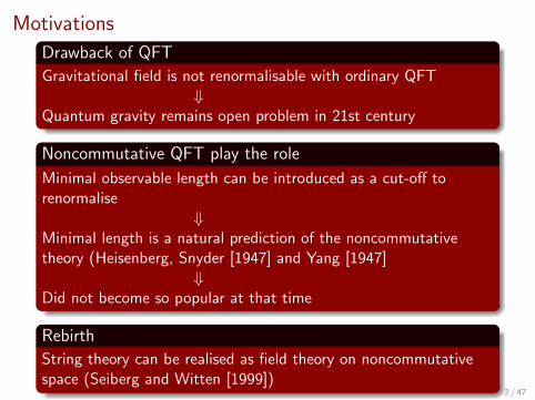
Drawback of QFT

Gravitational field is not renormalisable with ordinary QFT⇓

Quantum gravity remains open problem in 21st century

Noncommutative QFT play the role

Minimal observable length can be introduced as a cut-off torenormalise

⇓Minimal length is a natural prediction of the noncommutativetheory (Heisenberg, Snyder [1947] and Yang [1947]

⇓Did not become so popular at that time

Rebirth

String theory can be realised as field theory on noncommutativespace (Seiberg and Witten [1999])

2 / 47

Noncommutative spaces

• Flat (abelian) noncommutative space

[xµ, xν ] = iθµν , [xµ, pν ] = i~δµν and [pµ, pν ] = 0

Nonvanishing θµν breaks Lorentz-Poincare symmetry

• Snyder’s Lorentz covariant version

[xµ, xν ] = iθ (xµpν − xνpµ)

[xµ, pν ] = i~ (δµν + θpµpν)

[pµ, pν ] = 0

However, Poincare symmetry is still violated

• Poincare symmetries were deformed to make the algebracompatible with Snyder’s version [R. Banerjee, S. Kulkarni, S.Samanta; JHEP 2006, 077 (2006)].

3 / 47

q-deformed noncommutative spaces

• Deformation on Heisenberg’s canonical commutation relations

PX − qXP = i~

• Deformation on commutation relation between creation andannihilation operator

AA† − q2A†A = 1

Why deformation?

X = α(A† + A

), P = iβ

(A† − A

), α, β ∈ R

Constraints

α =~

2β, q = e2τβ2

, τ ∈ R+

Non-trivial limit β → 0

[X ,P] = i~(1 + τP2

).

4 / 47

Minimal lengthUncertainty relation:

∆A∆B ≥ 1

2|〈[A,B]〉|

• Standard case: [A,B] = Constant; give up knowledge aboutB, for ∆A = 0

• Noncommutative case: [A,B] ≈ B2; give up knowledge alsoabout B, for ∆A 6= 0

For the case:

[X ,P] = i~(1 + τP2

), ∆X∆P ≥ ~

2

[1 + τ (∆P)2 + τ〈P〉2

]⇒ Minimal length

∆Xmin = ~√τ√

1 + τ〈P2〉

from minimizing with (∆A)2 = 〈A2〉 − 〈A〉25 / 47

Flat noncommutative spaces in 3D

[x0, y0] = iθ1, [x0, z0] = iθ2, [y0, z0] = iθ3,[x0, px0 ] = i~, [y0, py0 ] = i~, [z0, pz0 ] = i~ for θ1, θ2, θ3 ∈ R

Linear Ansatz:

ϕi =3∑

j=1

κij aj + λija†j , for ~ϕ = {x0, y0, z0, px0 , py0 , pz0}

⇒ 72 free parameters

Utilize PT -symmetry to reduce number ofparameters

6 / 47

PT -symmetric flat noncommutative spaces

PT ± : x0 → ±x0, y0 → ∓y0, z0 → ±z0, i → −i ,px0 → ∓px0 , py0 → ±py0 , pz0 → ∓pz0 , θ2 = 0

PT θ± : x0 → ±x0, y0 → ∓y0, z0 → ±z0, i → −i ,px0 → ∓px0 , py0 → ±py0 , pz0 → ∓pz0 , θ2 → −θ2

PT xz : x0 → z0, y0 → y0, z0 → x0, i → −i ,px0 → −pz0 , py0 → −py0 , pz0 → −px0

PT ±-symmetric Ansatz

a1 = α1x0 + iα2y0 + α3z0 + iα4px0 + α5py0 + iα6pz0 ,

a2 = α7x0 + iα8y0 + α9z0 + iα10px0 + α11py0 + iα12pz0 ,

a3 = α13x0 + iα14y0 + α15z0 + iα16px0 + α17py0 + iα18pz0

7 / 47

Solution:

x0 =α9α17 − α11α15

2 detM1a+

1 +α5α15 − α3α17

2 detM1a+

2 +α3α11 − α5α9

2 detM1a+

3 ,

y0 =α10α18 − α12α16

2i detM2a−1 +

α6α16 − α4α18

2i detM2a−2 +

α4α12 − α6α10

2i detM2a−3 ,

z0 =α11α13 − α7α17

2 detM1a+

1 +α1α17 − α5α13

2 detM1a+

2 +α5α7 − α1α11

2 detM1a+

3 ,

px0 =α12α14 − α8α18

2i detM2a−1 +

α2α18 − α6α14

2i detM2a−2 +

α6α8 − α2α12

2i detM2a−3 ,

py0 =α7α15 − α9α13

2 detM1a+

1 +α3α13 − α1α15

2 detM1a+

2 +α1α9 − α3α7

2 detM1a+

3 ,

pz0 =α8α16 − α10α14

2i detM2a−1 +

α4α14 − α2α16

2i detM2a−2 +

α2α10 − α4α8

2i detM2a−3

with

a±i = ai ± a†i ,

(Ml)jk = 6j + 2k + l − 8 for l = 1, 2.

8 / 47

q-deformed noncommutative spaces

Deformed oscillator algebras

AiA†j − q2δijA†jAi = δij ,

[A†i ,A

†j

]= [Ai ,Aj ] = 0, i , j = 1, 2, 3; q ∈ R

The limit q → 1 gives standard Fock space Ai → ai :[ai , a

†j

]= δij , [ai , aj ] =

[a†i , a

†j

]= 0, i , j = 1, 2, 3

q-deformed Fock space representation (1D):

|n〉q =

(A†)n√

[n]q!|0〉, 〈0|0〉 = 1, A|0〉 = 0,

A†|n〉q =√

[n + 1]q |n + 1〉q, A|n〉q =√

[n]q |n − 1〉q

⇒ [n]q :=1− q2n

1− q2, where [n]q! =

n∏k=1

[k]q .

9 / 47

Noncommutative spaces from oscillator algebras

PT ±-symmetric Ansatz:

X = κ1(A†1 + A1) + κ2(A†2 + A2) + κ3(A†3 + A3),

Y = i κ4(A†1 − A1) + i κ5(A†2 − A2) + i κ6(A†3 − A3),

Z = κ7(A†1 + A1) + κ8(A†2 + A2) + κ9(A†3 + A3),

Px = i κ10(A†1 − A1) + i κ11(A†2 − A2) + i κ12(A†3 − A3),

Py = κ13(A†1 + A1) + κ14(A†2 + A2) + κ15(A†3 + A3),

Pz = i κ16(A†1 − A1) + i κ17(A†2 − A2) + i κ18(A†3 − A3),

with κi = κi√

~/mω for i = 1, ...., 9κi = κi

√~mω for i = 10, ...., 18

Note: X ,Y ,Z ,PX ,PY ,PZ are non-Hermitian in usual space

10 / 47

Compute non-Hermitian commutators:

[X ,Y ] = 2i∑3

j=1κj κ3+j

[1 +

(q2 − 1

)]A†jAj ,

[Y ,Z ] = −2i∑3

j=1κ3+j κ6+j

[1 +

(q2 − 1

)]A†jAj ,

[X ,Px ] = 2i∑3

j=1κj κ9+j

[1 +

(q2 − 1

)]A†jAj ,

[Y ,Py ] = −2i∑3

j=1κ3+j κ12+j

[1 +

(q2 − 1

)]A†jAj ,

[Z ,Pz ] = 2i∑3

j=1κ6+j κ15+j

[1 +

(q2 − 1

)]A†jAj ,

[Px ,Py ] = −2i∑3

j=1κ9+j κ12+j

[1 +

(q2 − 1

)]A†jAj ,

[Py ,Pz ] = 2i∑3

j=1κ12+j κ15+j

[1 +

(q2 − 1

)]A†jAj ,

[X ,Pz ] = 2i∑3

j=1κj κ15+j

[1 +

(q2 − 1

)]A†jAj ,

[Z ,Px ] = 2i∑3

j=1κ6+j κ9+j

[1 +

(q2 − 1

)]A†jAj ,

[X ,Z ] = [Px ,Pz ] = [X ,Py ] = [Y ,Px ] = [Y ,Pz ] = [Z ,Py ] = 011 / 47

A particular PT ±-symmetric solution

κ1 = κ4 = κ5 = κ8 = κ10 = κ12 = κ13 = κ14 = κ17 = κ18 = 0

[X ,Y ] =2iθ1

1 + q2+ i

θ1

~L

(mω

2κ26

Y 2 +2κ2

6

mωP2y

),

[Y ,Z ] =2iθ3

1 + q2+ i

θ3

~L

(mω

2κ26

Y 2 +2κ2

6

mωP2y

),

[X ,Px ] =2i~

1 + q2+ i2mωL

(κ2

11X2 +

P2x /4

m2ω2κ211

+θ2

1κ211P

2y

~2+κ2

11XPy

~/(2θ1)

),

[Y ,Py ] =2i~

1 + q2+ i2mωL

(1

4κ26

Y 2 +κ2

6

m2ω2P2y

),

[Z ,Pz ] =2i~

1 + q2+ i2mωL

(Z 2

4κ27

+κ2

7

m2ω2P2z +

θ23

4~2κ27

P2y −

θ3

2~2κ27

ZPy

),

where L = (q2 − 1)/(q2 + 1), with constraints

κ2 =~

2κ11, κ3 =

θ1

2κ6, κ9 = − θ3

2κ6, κ15 = − ~

2κ6, κ16 =

~2κ7

.12 / 47

Reduced three dimensional solution for q → 1

• Set κ11 = κ6, κ7 = 1/2κ6, q = Exp(2τκ26), then κ6 → 0:

[X ,Y ] = iθ1

(1 + τY 2

), [Y ,Z ] = iθ3

(1 + τY 2

),

[X ,Px ] = i~(1 + τP2

x

), [Y ,Py ] = i~

(1 + τY 2

),

[Z ,Pz ] = i~(1 + τP2

z

),

where τ = τmω/~, τ = τ/(mω~)

• Representation in flat noncommutative spaces:

X = (1 + τp2x0

)x0 + θ1~

(τp2

x0− τy2

0

)py0 , Px = px0 ,

Z = (1 + τp2z0

)z0 + θ3~(τy2

0 − τp2z0

)py0 , Pz = pz0 ,

Py = (1 + τy20 )py0 , Y = y0.

• Bopp shift to standard canonical variables:x0 → xs − θ1

~ pys , y0 → ys , z0 → zs + θ3~ pys ,

px0 → pxs , py0 → pys , pz0 → pzs

13 / 47

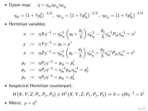
• Dyson map: η = ηy0ηPx0ηPz0

ηy0 =(1 + τy2

0

)−1/2, ηPx0

=(1 + τp2

x0

)−1/2, ηPz0

=(1 + τp2

z0

)−1/2

• Hermitian variables:

x := ηXη−1 = η−1Px0

(x0 +

θ1

~

)η−1Px0− θ1

~η−1y0

Py0η−1y0

= x†

y := ηY η−1 = y0 = y †

z := ηZη−1 = η−1Pz0

(z0 −

θ3

~

)η−1Pz0

+θ3

~η−1y0

Py0η−1y0

= z†

px := ηPxη−1 = px0 = p†x

py := ηPyη−1 = η−1

y0py0η

−1y0

= p†y

pz := ηPzη−1 = pz0 = p†z

• Isospectral Hermitian counterpart:

H (X ,Y ,Z ,Px ,Py ,Pz) 6= H† (X ,Y ,Z ,Px ,Py ,Pz)⇒ h = ηHη−1 = h†

• Metric: ρ = η2

14 / 47

Harmonic oscillators on a noncommutative space1D harmonic oscillator:

H =P2

2m+

mω2

2X 2 = H1D

ho +mω2

2

(τp2

s x2s + τxsp

2s xs + τ2p2

s xsp2s xs)

⇒ Non-Hermitian but PT ±-symmetricSolved exactly in p-space, i.e. xs → i~∂ps :

ψ2n−i (z) = c1

2n−i∑k=i

zk(z2 − 1)ν−2n−1+i

2

k+i−22∏

l=i

2(n − l)(2n + 2ν − 2l + 1)

k!(−1)1+i (1− z2)ν

,

En = ω~(

1

2+ n

)√1 +

τ2

4+ τ

ω~4

(1 + 2n + 2n2) for n ∈ N0

ψ2n−i (z) vanishes as |z | → ∞, if ν > −1, guaranteed for τmω > 0ψ2n−i (z)→ square integrable and forms orthonormal basis.

η =(1 + τP2

)−1/2

15 / 47

Exact treatment is always difficultPerturbation theory:

E(p)n = E

(0)n + E

(1)n + E

(2)n +O(τ3) with

E(0)n = ω~

(n +

1

2

),

E(1)n =

τω~4

(1 + 2n + 2n2

)+τ2ω~

16

(3 + 8n + 6n2 + 4n3

),

E(2)n = −1

8τ2ω~

(1 + 3n + 3n2 + 2n3

)Upto order τ3, the energy matches exactly with the exact case

Higher dimensional models have also been treated similarly, forinstance in 2D and in 3D

16 / 47

Minimal lengths, areas and volumes

Uncertainty relation:

∆A∆B ≥ 1

2|〈[A,B]〉ρ|

For special solution with q → 1:

∆Xmin = |θ1|√τ + τ2 〈Y 〉2ρ, ∆Ymin = 0, ∆Zmin = |θ3|

√τ + τ2 〈Y 〉2ρ,

∆Xmin = ~√τ + τ τ 〈Y 〉2ρ, ∆Ymin = 0, ∆Zmin = ~

√τ + τ τ 〈Y 〉2ρ,

∆ (Px)min = 0, ∆ (Py )min = ~√τ + τ2 〈Y 〉2ρ, ∆ (Pz)min = 0.

17 / 47

Before taking the limit:

∆Ymin = |κ6|

√1

2(q2 − q−2) + (q − q−1)2

(1

4κ26

〈Y 〉2ρ +κ2

6

~2

⟨P2y

⟩ρ

),

Similar expressions can be found for X and Z .Absolute minimal lengths:

∆X0 =1

2√

2

∣∣∣∣ θ1

κ6

∣∣∣∣Q, ∆Y0 =|κ6|√

2Q, ∆Z0 =

1

2√

2

∣∣∣∣ θ3

κ6

∣∣∣∣Q,where Q :=

√q2 − q−2

Absolute minimal uncertainty volume:

∆V0 =1√2

∣∣∣∣θ1θ3

κ6

∣∣∣∣ (q2 − q−2)3/2

.

-Similarly for the momenta

18 / 47

Different types of representations

[X ,P] = i~(1 + τP2

)non-Hermitian: X(1) = (1 + τp2)x , P(1) = p,

Hermitian: X(2) = (1 + τp2)1/2x(1 + τp2)1/2, P(2) = p,

Hermitian: X(3) = x , P(3) =1√τ

tan(√

τp),

non-Hermitian: X(4) = ix(1 + τp2)1/2, P(4) = −ip(1 + τp2)−1/2,

Incorrect: X(4′) = x(1 + τp2)1/2, P(4) = p(1 + τp2)−1/2

[P. G. Castro, R. Kullock and F. Toppan:J. Math. Phys. 52, 062105 (2011)]

How are these representations related?

19 / 47

Construction of solvable non-Hermitian potentials

H(p)ψ(p) = Eψ(p) ⇔ −f (p)ψ′′(p)+g(p)ψ′(p)+h(p)ψ(p) = Eψ(p)

Transformation:

ψ(p) = eχ(p)φ(p), χ(p) =

∫f ′(p) + 2g(p)

4f (p)dp, q =

∫ √f (p)dp,

H(q)ψ(q) = Eψ(q) ⇔ −φ′′(q) + V (q)φ(q) = Eφ(q),

so that the potential, V (q) =4g2 + 3 (f ′)2 + 8gf ′

16f− f ′′

4− g ′

2+ h

∣∣∣∣∣q

.

Factorize the wave function further:

φ(q) = v(q)F [w(q)],

where F [w(q)] is introduced as a special function20 / 47

The Ansatz converts the potential equation back into

F ′′(w) + Q(w)F ′(w) + R(w)F (w) = 0,

where, Q(w) :=2v ′

vw ′+

w ′′

(w ′)2and R(w) :=

E − V (q)

(w ′)2+

v ′′

v (w ′)2.

1st relation gives:

v(q) =(w ′)−1/2

exp

[1

2

∫ w(q)

Q(w)dw

],

Eliminating v(q) in the 2nd relation:

E−V (q) =w ′′′

2w ′−3

4

(w ′′

w ′

)2

+(w ′)2

R(w)−(w ′)2 Q ′(w)

2−(w ′)2 Q2(w)

4,

with known Q(w),R(w),F [w(q)]⇒ compute w(q)General formula for the metric:

ρ(p) = %(p)e−2Reχ(p) |v(p)|−2 dw

dp.

21 / 47

Nc harmonic oscillator in different representations

Representation 1:

H(1)(p) =p2

2m+

mω2

2

(x2 + τp2x2 + τxp2x + τ2p2xp2x

),

In momentum space (x → i~∂p)

f (p) =mω2~2

2(1 + τp2)2, g(p) = −τ~ωp(1 + τp2), h(p) =

p2

2m.

Transformations:

ψ(p) = φ(p), q =

√2

τω~arctan

(√τp),

Such that

V (q) =~ω2τ

tan2

(√τω~

2q

).

22 / 47

Assume F (w)⇒ associated Legendre polynomial Pµν (w)

Q(w) =2w

w2 − 1and R(w) =

ν(ν + 1)

1− w2− µ2

(1− w2)2

so that,

E − ~ω2τ

tan2

(√τω~

2q

)

=(w ′)2

(ν2 + ν + 1

1− w2+

w2 − µ2

(1− w2)2

)− 3 (w ′′)2

4 (w ′)2+

w ′′′

2w ′

Assume first term on R.H.S constant, (w ′)2 /(1− w2) = c ∈ R+

w(q) = sin(√cq), so that

ψn(p) =1√Nn

1

(1 + τp2)1/4Pµ−n−µ−

( √τp√

1 + τp2

),

En = ω~(

1

2+ n

)√1 +

τ2

4+τω~

4(1 + 2n + 2n2).

23 / 47

Representation 2:

As H(2) = ρ1/2H(1)ρ−1/2, ψn(2)

= ρ−1/2ψn(1), En(2)

= En(1)

Representation 3:

H(3)(p) = H(1)(q = p√

2/m/~ω), ∴ φ(q = p√

2/m/~ω)

Representation 4’:

E = ~ω/2τ − c/4(1 + 2ν)2 ⇐ Not bounded from below

Representation 4 makes it physical.For all representations:⟨

ψ(i)

∣∣F (P(i),X(i)

)ψ(i)

⟩ρ(i)

=1

N

∫ 1

−1F

[z√

τ(1− z2), i~√τ(1− z2)∂z

] ∣∣∣Pµ−m−µ− (z)∣∣∣2 dz

24 / 47

Klauder coherent states

|J, γ, φ〉 =1

N (J)

∞∑n=0

Jn/2e−iγen√ρn

|φn〉, J ∈ R+0 , γ ∈ R.

with

h|φn〉 = ~ωen|φn〉, ρn =n∏

k=1

ek and N 2(J) =∞∑k=0

Jk

ρk,

Basis properties:

• Continuous in J, γ

• Provide a resolution of the identity

• Temporarily stable

• Satisfy action identity

〈J, γ, φ|H|J, γ, φ〉η = 〈J, γ, φ|h|J, γ, φ〉 = ~ωJ

J. R. Klauder, Annals Phys. 237, 147− 160 (1995)

25 / 47

Generalised Heisenberg’s uncertainty relation

For a measurement of two observables A and B we have:

∆A∆B ≥ 1

2

∣∣∣〈J, γ,Φ| [A,B] |J, γ,Φ〉η∣∣∣

Uncertainties:

∆A = 〈J, γ,Φ|A2 |J, γ,Φ〉η − 〈J, γ,Φ|A |J, γ,Φ〉2η

Ehrenfest theorem

i~d

dt〈J, γ + tω,Φ|A |J, γ + tω,Φ〉η = 〈J, γ + tω,Φ| [A,H] |J, γ + tω,Φ〉η

Time evolution

e iHt/~|J, γ,Φ〉 = |J, γ + tω,Φ〉

26 / 47

1D perturbative noncommutative harmonic oscillator

H =P2

2m+

mω2

2X 2 − ~ω

(1

2+τ

4

)defined on the noncommutative space

[X ,P] = i~(1 + τP2

), X = (1 + τp2)x , P = p

First order perturbation theory

En = ~ωen = ~ωn[1 +

τ

2(1 + n)

]+O(τ2)

|φn〉 = |n〉 − τ

16

√(n − 3)4 |n − 4〉+

τ

16

√(n + 1)4 |n + 4〉+O(τ2)

Pochhammer function (x)n := Γ(x + n)/Γ(x)

ρn =1

2nτnn!

(2 +

2

τ

)n

, N 2(J) = eJ(

1− τJ − τ

4J2)

+O(τ2)

27 / 47

The K-states saturate the generalized uncertainty relation

∆X 2 = 〈J, γ,Φ|X 2 |J, γ,Φ〉η − 〈J, γ,Φ|X |J, γ,Φ〉2η

=~

2mω[1 + τ (1 + J(2− 2γ sin 2γ − cos 2γ))]

∆P2 = 〈J, γ, φ| p2 |J, γ, φ〉 − 〈J, γ, φ| p |J, γ, φ〉2

=~mω

2[1− τJ(cos 2γ − 2γ sin 2γ)]

Therefore

∆X∆P =~2

[1 +

τ

2

(1 + 4J sin2 γ

)]=

~2

(1 + τ 〈J, γ,Φ|P2 |J, γ,Φ〉

)⇒ Squeezed coherent states

Strong disagreement with

[S. Gosh, P. Roy; Phys. Lett. B711, 423 (2012)]

28 / 47

1D non-perturbative noncommutative harmonic oscillator

Now consider deformed canonical commutation relations:

[X ,P] = i~ + iq2 − 1

q2 + 1

(mωX 2 +

1

mωP2

)Take

X = α(A† + A

)and P = iβ

(A† − A

)with α = 1

2

√1 + q2

√~

mω and β = 12

√1 + q2

√~mω

Non-perturbative NCHO

H = ~ω(A†A + 1

), En = ~ωen = ~ω[n]q, |φn〉 = |n〉q

H =2

(1 + q2)2

[mω2X 2 +

1

mP2 +

~ω8

(q4 − 2q2 − 3

)]

30 / 47

Hermitian representation:

A =i√

1− q2

(e−i x − e−i x/2e2τ p

), A† =

−i√1− q2

(e i x − e2τ pe i x/2

)with x = x

√mω/~ and p = p/

√mω~ , [x , p] = i~

Non-Hermitian representation:

A =1

1− q2Dq, and A† = (1− x)− x(1− q2)Dq

Jackson derivatives Dqf (x) := [f (x)− f (q2x)]/[x(1− q2)]

Generalised uncertainty relation for Hermitian representation:

∆X∆P||J,γ〉q ≥1

2

∣∣∣∣(q〈J, γ| [X ,P] |J, γ〉q)η

∣∣∣∣are shown to hold, but are saturated only for t = 0

Ehrenfest theorem are also shown to hold for both X and P31 / 47

Revival structureDynamics of classical systems with equidistant energy lavels:

Tcl =2π~∆En

Non-equidistant energy lavels: Trev ⇒ regains its original structure

Revival structure requires

• Large number of waves from highly excited discrete states

• Strong localisation of the wave packet

Localisation

Given: |ψ(t)〉 =∑n≥0

cne−iEnt/~|φn〉 with

∞∑n=0

|cn|2 = 1

Compare: |cn|2 ⇐⇒ 〈n〉ke−〈n〉k!

Deviation measured by: Mandel parameter Q = (∆n)2

〈n〉 − 1Q = 0⇒ Poissonian, Q < 0⇒ Sub, Q > 0⇒ Super

32 / 47

Considering the wave packet strongly weighted around 〈n〉:Expand energy eigenvalue in Taylor series:

En ' En + E ′n (n − n) +1

2!E ′′n (n − n)2 +

1

3!E ′′′n (n − n)3 + .... ,

so that

Tcl =2π~|E ′n|

, Trev =2π~× 2!

|E ′′n |Tsuprev =

2π~× 3!

|E ′′′n |.

Classical description

Evidence: Revival structure (non-equidistant energy lavels)Visualised by autocorrelation function:

A(t) = 〈ψ(0)|ψ(t)〉 =∞∑n=0

|cn|2e−iEnt/~ .

Numerically |A(t)|2 varies between 0 and 1

33 / 47

Fractional revival of perturbative NCHO

Klauder coherent states: |J, γ, φ〉 =∑∞

n=0 cn(J)e−iEnt/~|φn〉Weighting function: cn(J) = Jn/2

N (J)√ρn

〈n〉 = J−τ(J +

J2

2

)+O(τ2),

⟨n2⟩

= J+J2−τ(J + 3J2 + J3

)+O(τ2)

∆n2 =⟨n2⟩− 〈n〉2 = J − τ

(J + J2

)+O(τ2)

Mandel parameter:

Q :=∆n2

〈n〉− 1 = −Jτ

2+O(τ2) < 0,

⇒ Sub-Poissonian statistics (Strong localisation)

34 / 47

Weighting function

0.0 2.5 5.0 7.5 10.00.0

0.1

0.2

0.3

0.4

J = 1.5 J = 3

------- J = 4.5

(a)

|c(J

)|2

n 0 5 10 15 20 250.00

0.06

0.12

0.18

0.24 J = 3 J = 6

- - - - J = 15

(b)

|c(J

)|2

n

(a) τ = 0.1 with 〈n〉 = 1.24, 2.25, 3.04(b) τ = 0.01 with 〈n〉 = 2.93, 5.76, 13.72

35 / 47

Autocorrelation function

0 50 100 150 200 2500.00

0.25

0.50

0.75

1.00

J = 1.5(a)A(t)

t 0 500 1000 1500 2000 25000.00

0.25

0.50

0.75

1.00

Trev/3

Trev/4

Trev/8

Trev/6

J = 6(b)A(t)

t

Trev/2

(a) J = 1.5, τ = 0.1, ω = 0.5, ~ = 1, γ = 0,Tcl = 10.05,Trev = 251.32(b) J = 6, τ = 0.01, ω = 0.5, ~ = 1, γ = 0,Tcl = 11.74,Trev = 2513.27

Tcl =2π

ω− τ

ω(1 + 2J)π, and Trev =

4π

ωτ

36 / 47

Fractional super-revival of non-perturbative NCHO

En = ~ω[n]q, [n]q =1− q2n

1− q2⇒ dkEn

dnk6= 0 for k = 1, 2, 3..

⇒ Infinite many revival

Tcl =π

ω

∣∣∣∣ q2 − 1

q2n ln q

∣∣∣∣ , Trev =π

ω

∣∣∣∣ q2 − 1

q2n ln2 q

∣∣∣∣ , Tsuprev =3π

2ω

∣∣∣∣ q2 − 1

q2n ln3 q

∣∣∣∣

0 1 2 3 4 5 60.00

0.25

0.50

0.75

1.00

J = 6(a)A(t)

t 0 250 500 750 1000 12500.00

0.25

0.50

0.75

1.00

Trev/3

Trev/4

Trev/8

Trev/6

J = 6(b)A(t)

t

Trev/2

0 100000 200000 300000 4000000.00

0.25

0.50

0.75

1.00 Tsuprev/3Tsuprev/6

J = 6(c)A(t)

t

Tsuprev/2

q = e−0.005, J = 6, n = 6.1875(a) Tcl = 6.65 (b) Trev = 1330.19 (c) Tsuprev = 3999056

37 / 47

Yet another efficient method

Quality of coherent states

• Solve canonical equations of motion ⇒ Draw the dynamicsof classical particles

• Utilize Bohmian mechanics ⇒ Draw the dynamics ofcoherentt states

• Compare directly ⇒ Study quality of the coherent states

Bohmian mechanics (real case):

Time dependent Schrodinger equation :

i~∂ψ(x , t)

∂t= − ~2

2m

∂2ψ(x , t)

∂x2+ V (x)ψ(x , t)

WKB polar decomposition :

ψ(x , t) = R(x , t)ei~S(x ,t), R(x , t),S(x , t) ∈ R

Substitute ψ(x , t) in Schrodinger equation ⇒ separate real andimaginary part :

38 / 47

Real Bohmian

St +(Sx)2

2m+ V (x)− ~2

2m

Rxx

R= 0 ⇐ Quantum Hamilton-Jacobi equation

mRt + RxSx +1

2RSxx = 0 ⇐ Continuity equation

∗ Velocity :

mv(x , t) = Sx =~2i

[ψ∗ψx − ψψ∗x

ψ∗ψ

]∗ Quantum potential :

Q(x , t) = − ~2

2m

Rxx

R=

~2

4m

[(ψ∗ψ)2

x

2 (ψ∗ψ)2−

(ψ∗ψ)xxψ∗ψ

]∗ Effective potential Veff(x , t) = V (x) + Q(x , t).∗ Two options to compute quantum trajectories :

1. Solve ⇒ v(x , t)2. Solve ⇒ mx = −∂Veff/∂x

39 / 47

Bohmian mechanics (complex case)

∗ Decompose :

ψ(x , t) = ei~ S(x ,t), S(x , t) ∈ C

∗ Substitute ψ(x , t)⇒ time dependent Schrodinger equation :

St +(Sx)2

2m+ V (x)− i~

2mSxx = 0

∗ Velocity :

mv(x , t) = Sx =~i

ψx

ψ

∗ Quantum potential :

Q(x , t) = − i~2m

Sxx = − ~2

2m

[ψxx

ψ− ψ2

x

ψ2

]∗ Less explored in the literature

40 / 47

Application : Poschl-Teller model (real case)

φn(x) =1√Nn

cosλ( x

2a

)sinκ

( x

2a

)2F1

[−n, n + κ+ λ; k +

1

2; sin2

( x

2a

)]Stationary state Bohmian :

v(t) = 0 ⇐ Not the behaviour of a classical particle.Klauder coherent state :

ψJ(x , t) :=1

N (J)

∞∑n=0

Jn/2 exp(−iωten)√ρn

φn(x)

ρn = n!(n + κ+ λ)n, N 2(J) = 0F1 (1 + κ+ λ; J)Classical solution :

x(t) = a arccos

[α− β

2+√γ cos

(√2E

m

t

a

)], α, β, γ constant

41 / 47

0 . 0 0 . 2 0 . 4 0 . 6 0 . 8 1 . 02 . 0 0

2 . 0 1

2 . 0 2

2 . 0 3

2 . 0 4

2 . 0 5

x ( t )

t

( a )

0 5 10 15 20 252

3

4

5

6

(c)

J = 20 J = 10 J = 2 J = 20.2846

x(t)

t

(a) Classical trajectories (c) Trajectories of coherent states

• Qualitatively not identical !!• Let us look at the uncertainty• Let us look at the behaviour of |ψ(x , t)|2 with time too

42 / 47

0 5 1 0 1 5 2 0 2 50

1

2

3

4

5

6

7

Q = - 0 . 3 0 7 5 9 3 Q = - 0 . 1 4 9 5 2 3 Q = - 0 . 0 4 2 5 5 5

∆x ∆p

t

( a )

0 1 2 3 4 5 60.0

0.2

0.4

0.6

0.8

t = 0t = 1t = 10t = 20t = 30

|(x

,t)|2

x

(b)

• Not a squeezed coherent state, ∆x∆p ≫ }/2 !!• Shape of the wave packet changes with time, i.e. not a classical particle!!• Q = −0.307593,−0.149523,−0.042555⇐ Sub-Poissonian• Q(J, κ+ λ) = J

2+κ+λ0F1(3+κ+λ;J)

0F1(2+κ+λ;J) −J

1+κ+λ0F1(2+κ+λ;J)

0F1(1+κ+λ;J)• Adjust κ, λ and J, so that Q→ 0⇐ Poissonian

43 / 47

0 5 10 15 20 25

0.5100

0.5103

0.5106

0.5109

0.5112

x p

t

Q= -0.000054529 Q= -0.000013634 Q= -0.000002726

(a)

0.0 0.4 0.8 1.2

0.5000055

0.5000070

0 1 2 3 4 5 60

1

2

3

t = 0 , J = 0 . 0 0 2 2 9 0 6 t = 0 . 6 5 , J = 0 . 0 0 2 2 9 0 6 t = 0 , J = 2 t = 4 , J = 2|Ψ

(x,t)|2

x

( b )

Two sets: κ = 90, λ = 100, J = 2, 0.5, 0.1κ = 2, λ = 3, J = 2, 0.5, 0.1

0.0 0.2 0.4 0.6 0.8 1.02.00

2.01

2.02

2.03

2.04

2.05 (a)

J = 2.0 J = 0.5 J = 0.1

x(t)

t 0 5 10 15 20 25 302.00

2.01

2.02

2.03

2.04

2.05

2.06 (b)

J = 0.0022906 J = 0.00057265 J = 0.000114531

x(t)

t44 / 47

Classical and Klauder state in complex plane

- 0.9

- 0.9 - 0.9

- 0.9 - 0.9

- 0.9

- 0.9

- 0.9

- 0.9

- 0.9

- 0.8 - 0.8

- 0.8 - 0.8- 0.8

- 0.8

- 0.8- 0.8

- 0.8- 0.8

- 0.7

- 0.7

- 0.6

- 0.6

- 0.5

- 0.5

- 0.4

- 0.4

- 0.3- 0.3- 0.3 - 0.3 - 0.3

- 0.3- 0.2- 0.2

- 0.2- 0.2

- 0.2 - 0.1- 0.1- 0.1- 0.1 - 0.1

xi

xr

(a)

- 20 - 15 - 10 - 5 0 5

- 3

- 2

- 1

0

1

2

3

- 0.8

- 0.8

- 0.8

- 0.8

- 0.8- 0.8

- 0.8

- 0.8

- 0.8

- 0.6- 0.6

- 0.6- 0.6

- 0.6

- 0.6

- 0.6

- 0.6

- 0.6

- 0.4- 0.4- 0.4

- 0.4 - 0.4

- 0.4

- 0.4- 0.4

- 0.4

- 0.2

- 0.2

- 0.2 - 0.2

- 0.2- 0.2

- 0.2 - 0.2

- 0.2

00

00

0

0

00 0

0

0

0

0

0

0.2

0.20.2

0.2

0.20.2

0.2 0.2

0.2

0.4

0.4

0.4

0.4

0.4 0.4

0.4

0.4

0.4

0.6

0.60.6

0.6

0.6

0.6

0.6

0.6

0.6

0.80.80.8

0.8

0.8

0.8

0.8

0.8

0.8

xr

xi (b)

- 20 - 15 - 10 - 5 0 5

- 3

- 2

- 1

0

1

2

3

Sub-Poissonian regime, Q < 0

45 / 47

- 2500

- 2500- 2500

- 2500- 2500

- 2500

- 2000

- 2000

- 2000

- 2000

- 2000

- 2000

- 1500

- 1500

- 1500

- 1500

- 1500

- 1500

- 1000 - 1000

- 1000 - 1000

- 1000

- 1000

- 500

- 500

0

00

500

500500

(a)xi

xr

- 6 - 4 - 2 0 2 4 6

- 3

- 2

- 1

0

1

2

3

- 2500

- 2500

- 2500

- 2500

- 2000

- 2000- 2000

- 2000- 1500

- 1500- 1500

- 1500- 1000

- 1000

- 1000

- 1000

- 500

- 500

- 500

- 500

00

0

0 0

0

0

500

500

500

500

(b)xi

xr

- 6 - 4 - 2 0 2 4 6

- 3

- 2

- 1

0

1

2

3

Quasi-Poissonian regime, Q → 0Perfect matching : Classical ⇐⇒ Klauder coherent state

46 / 47

Conclusions• Constructed noncommutative models both perturbatively and

exactly.

• PT -symmetry has been utilized to obtain Hermitiancounterparts of non-Hermitian models.

• Analytical expression of the metric is found for a class ofnon-Hermitian models.

• Computed minimal volume.

• Constructed Klauder coherent states for both perturbative andnonperturbative noncommutative models.

• Utilised revival structure to study the qualities of the coherentstates.

• Qualities have been investigated furthur by using Bohmianmechanics.

Thank you for your attention47 / 47

solvable models on noncommutative spaces with minimal length uncertainty relations

Science

det m1

det m2

x p x p x

px0 px0

px0 pz0

pz0 pz0

py0 py0

p2 p