explicitly solvable first order diﬀerential equationsmzhan/chapter2.pdf · chapter 1 explicitly...

CHAPTER 1

Explicitly Solvable First Order DifferentialEquations

In this chapter we will introduce the first order differential equationsand several type of it that can be solved explicitly using integrationmethods covered in standard Calculus course.

From Calculus, we know that the derivative df(t)dt

of a function f(t)is the rate at which the quantity x = f(t) is changing with respectto the independent variable t. An equation relating an unknownfunction and one or more of its derivatives is called an differentialequation. Particulary, an equation of the form x′ = f(t, x) is called afirst order ordinary differential equation(ODE), more precisely a semilinear first order ordinary differential equation. In this chapter willwill demonstrate how to find explicit solution(s) to a given ODE . Ingeneral one can’t find explicit solution to a given ODE , but for specialtypes of f(t, x), we will have luck to do that.

Some clearance of notations is needed here.In x′ = f(t, x), t is the independent variable and x(t) is the unknown

function, x′ is dxdt

, the first derivative of x(t), and f(t, x) is a givenfunction of two variables t and x. So to find an explicit solution is tofind an formula for x(t) so that when substitute the formula in f(t, x),we will get an expression in t only that matches x′(t). For example, forexample, suppose we have f(t, x) = x+ t, our ODE reads, x′ = x+ t. Ifwe set x(t) = 2et− t− 1 then f(t, x) = x+ t = 2et− t− 1+ t = 2eT − 1and x′(t) = 2et− 1 so x′ = f(t, x) and x(t) = 2et− t− 1 is an solution.

On the other hand if we write y′ = f(x, y), then in this ODE , xis the independent variable, y(x) is the unknown function to be found,and y′ is dy

dx, the first derivative of y(x). So for y′ = y + x, we would

get an solution y(x) = ex − x− 1.Sometimes the independent variable does not appear in the equa-

tion such as y′ = f(y) or x′ = f(x) in those case, one could assume theindependent variable is either x (for y′ = f(y)) or t (for x′ = f(x)) andwrite the solution accordingly. Hence, for y′ = y one solution would bey(x) = ex and for x′ = x, one would write as solution as x(t) = et.

1

2 1. EXPLICITLY SOLVABLE FIRST ORDER DIFFERENTIAL EQUATIONS

Note 0.1. It is very important for students to know what variablerepresents an unknown function and what variable represents the in-dependent variable that the unknown function is defined with respectto.

1. Finding antiderivative using Mathcad

You can use Mathcad to find both definite and indefinite integral.To access those two operators, you can bring up the popup menu, (See

Figure 1. Calculus tool bar

chapter 1 for how to bring up the Calculus popup menu.) Click on the∫ b

asymbol to get the operator for definite integral and on the

∫symbol

to get the operator for the indefinite operator. Then just fill in theplace holders accordingly. For definite integral, hit = to get the valueand for indefinite integral, you need either

• Select the entire expression and from the Symbolics menufollowing the menu item evaluate to the symbolically(Or[Shift][F9]).

or

• Hold down the [Ctrl] key and press the [.] (period) key.

You can also access the integration operators by hot keys [Shift][F7]for definite integral and [Ctrl][I] for indefinite integral.

The integration operators appear on the workplace as shown in thefollowing diagram,

Now lets see some examples. The first example is for finding definiteintegral.

Example 1.1. Find the definite integral∫ 3

0(x5− e3x− sin(3x)) dx.

Solution At any blank space in the workplace of Mathcad , type[Shift][F7], that is hold the [Shift] key and press [F7] key to place thedefinite integration operator ∫

d

1. FINDING ANTIDERIVATIVE USING Mathcad 3

Figure 2. Integration Operators

. Click the upper limit place holder, type 3 and click the lower limitplace holder type 0. Now click the integrant place holder type

x^5 -e^3x -sin(3x)

notice you need it the space bar twice before -sin(3x) . Ofcourse you need hit space bar once before entering -e^3x to exit thepower mode. Finally in the integration variable place holder type x(seeFigure 2 for the position of each place holder.) Now hit [=] key if inautomatic mode or =[F9] otherwise to find the value −2.5× 103. a

The second example is for find indefinite integral.

Example 1.2. Find the definite integral∫

(√

x + 2−e3x−sin(3x)) dx.

Solution At any blank space in the workplace of Mathcad ,type [Ctrl][I], that is hold the [Ctrl] key and press [I] key to place theindefinite integration operator

∫d .

Click the integrant place holder and type

\x+2 -e^3x -sin(3x)

Notice you need to hit the space bar twice before -sin(3x) . Ofcourse you also need hit space bar twice too before entering -e^3x toexit the square root operator.

In general, you will need to hit the space bar as many timesan need to escape the power(subscript, division, etc.) modebefore you enter next term.

The backslash \ brings up the square root operator. Finally inthe integration variable place holder type x(see Figure 2 for the positionof each place holder.) Now hold down[Ctrl] to type [.] key and click on


any region outside the bounding box, if not in the auto executionmode hit [F9] too, to find the antiderivative∫ √

x + 2− e3x − sin(3x) dx → 2

3(x + 2)

32 − 1

3exp3x +

1

3cos(3x)

. Here exp represent exponential function. From Calculus, we knowthat∫ √

x + 2− e3x − sin(3x) dx =2

3(x + 2)

32 − 1

3exp3x +

1

3cos(3x) + C.

Mathcad omits the C for believing you know it! Remember C is im-portant when we try to find a particular solution for a given, so called,”initial” condition.

Example 1.3. Find a function x(t) such that x′(t) = 2t and x(0) =3.

Solution If we take antiderivative on both sides, we have∫x′(t) dt =

∫2t dt

which leads to

x(t) = t2 + C.(1)

Evaluate this x(t) at t = 0 we have

x(0) = 02 + C = C

So the requirement x(0) = 3 implies C = 3. Hence x(t) = t2 + 3.Notice if we drop the C from (1), we would not be able to find x(t)

that satisfies x(0) = 3! aThe problem of finding a particular solution with initial condition is

called initial value problem, which we will discuss in the later section. aPractice

1. Find the following definite integral using Mathcad .

(a)∫ 2

−1x3 − x cos(x2 + 1) dx

(b)∫ 4

1x3+4x−5

x+1dx

(c)∫ 0

−5e3x − x

x2+3dx

(d)∫ 10

−1x2 − x sec(x2 + 1) dx

2. Find the following indefinite integral using Mathcad .

(a)∫

x5 − x√

(x2 + 1) dx

(b)∫

x3+4x−5x2+1

dx

2. SEPARABLE EQUATIONS 5

(c)∫

x−3(x2+3)(x+5)

dx

(d)∫

x tan(x2 + 1) dx

2. Separable equations

If we let x be the independent variable and y be the dependentvariable, a separable ODE is given by,

y′ = f(x)g(y)

where both f and g are given one variable functions and y′ = dydx

is thederivative of y(x) with respect to x and y(x) is the unknown functionwe want to find out.

When g(y) ≡ 1, that is g(y) is a constant function whose value isalways 1, the separable ODE becomes

y′ = f(x)

, which is sometimes called integrable ODE . The general solution tothe integrable ODE is the antiderivative of f(x), i.e.

y(x) =

∫f(x) dx

So if we can find the antiderivative of f(x) we can find the explicitgeneral solution.

Example 2.1. Find solution y′ = x2 + 3

Solution The solution is,

y(x) =

∫x2 + 3 dx =

1

3x3 + 3x + C

. Here we used the power rule of antiderivative,∫

xn dx =xn+1

n + 1+ C.

To find the solution in Mathcad , you just click any blank area in theworkplace and type [Ctrl][I] to get the indefinite operator∫

d

and type x^2 +3 in the place holder for integrant and x in the inte-grating variable place holder. Then press [Ctrl][.] and click on anyregion outside the bounding box to get the result. Sometime youmight need to hit [F9] too if the auto execution mode is turn off. a


When g(y) is not a constant function, the general solution to

y′ = f(x)g(y)

is given by the equation∫dy

g(y)=

∫f(x) dx,(2)

which is obtained by dividing both sides of the equation by g(y) andthen taking antiderivative to both sides.

So one has to find two antiderivatives∫

dyg(y)

and∫

f(x) dx. Some-

times we can solution for y(x) explicit from the (2), sometimes we can’tfind explicit formula for y(x), in that case we say y(x) is an implicitlydefined function.

Notice, in the process of finding the general solution to the separableODE , we divide both sides of the equation by g(y), that implicitlyrequires that g(y) 6= 0. On the other hand if g(c) = 0 then y(x) = c isan solution to the separable equation

y′ = f(x)g(y)

This kind solutions are called stationary or steady-state solutions.Sometimes they are also called singular solution.

Example 2.2. In the study of Epidemics, the spread of disease ina population can be modelled by I ′ = (b(t)S(t) − r(t))I where S(t) isnumber of people that is susceptible to the disease but not infected yet.I(t) is number of people actually infected. b, r are proportional function.Now suppose S(t) = e−3t, b = t2, and r = 4, find all solutions.

Solution First notice that I(t) ≡ 0 is the steady-state solution.Then, to

I ′ =dI

dt= (b(t)S(t)− r(t))I,

divide its both sides by I, multiplying its both sides by dt and takingantiderivative we have∫

dI

I=

∫b(t)S(t)− r(t) dt

The left side is easy to find,∫dI

I= ln |I|+ C(3)

Plug in the given functions, we get the right hand side∫b(t)S(t)− r(t) dt =

∫t2e−3t − 4 dt

2. SEPARABLE EQUATIONS 7

Now open Mathcad window, click any blank area, type [Ctrl][I] to getthe antiderivative operator ∫

d

type t^2 *e^{-3t} - 4 in the integrant place holder (again usingspace bar to exit the power mode) and t in the other place holder, thentype [Ctrl][.], click any area outside the box. You will get∫

t2e−3t − 4 dt = −1

3t2e−3t − 2

9te−3t − 2

27e−3t − 4t + C(4)

Put (3) and (4) together, we have

ln |I(t)| = −13t2e−3t − 2

9te−3t − 2

27e−3t − 4t + C

Solve for I(t), we finally arrive at

I(t) = e−13t2e−3t− 2

9te−3t− 2

27e−3t−4t+C

= Ce−13t2e−3t− 2

9te−3t− 2

27e−3t−4t

aThe next example shows that sometimes we can find explicit for-

mula for the solution of an separable ODE .

Example 2.3. Find general solution of y′ = ex+2xsin(y)+3y2+3

Solution Write y′ as dydx

, multiply both sides of the equation by(sin(y) + 3y2 + 3)dy and take antiderivative, we have∫

sin(y) + 3y2 + 3 dy =

∫ex + 2x dx

Now using Mathcad or compute by hand, we find∫sin(y) + 3y2 + 3 dy = − cos(y) + y3 + 3y + C

and ∫ex + 2x dx = ex + x2 + C

So we have an implicitly defined solution y(x) by the equation

− cos(y) + y3 + 3y = ex + x2 + C

Here, we can’t find an explicit formula for y(t). a

Practice


Project

3. Linear equations and Bernoulli equations

3.1. Linear Equations. An ODE of form

y′ + a(x)y = b(x)

is called a linear equation. Any equation that can be converted intothis form can also be called a linear equation. Such as x2y′ + 4x2exy =

sin(x), which can be written as y′ + exy = sin(x)x2 , is a linear equation.

The general solution of the linear equation is

y(x) = eR

a(x) dx

( ∫b(x)e−

Ra(x) dx dx + C

)

Notice that C is inside the parenthesis. It is common mistake ofstudents forgetting multiplying C by e

Ra(x) dx.

Example 3.1. According to Newton’s law of cooling, the time rateof change of the temperature T (t) of a air conditioned house with ex-ternal temperature A(t) is proportional to the difference A − T . Thatis,

dT

t= k(A− T ),

where k is positive constant. Now, suppose A(t) = 80− 10 cos(ωt) findthe general solution.

Solution Since we want to use Mathcad to find the antiderivativefor us, the first thing is to find how to get the Greek letter ω. To getω, first bring the math tool bar from the View menu

Figure 3. Math Toolbar

3. LINEAR EQUATIONS AND BERNOULLI EQUATIONS 9

Click on the

Figure 4. Greek Letter Button

which will bring up

Figure 5. Greek Letter Bar

and select the ω letter.Now if we rewrite and put in A(t)

dT

t= k(A− T ),

we getdT

t= k(80− 10 cos(ωt))− kT,

and is a linear equation with a(t) = k and b(t) = k(80− 10 cos(ωt)), iteasy to see that

∫a(t) dt =

∫k dt = kt. Apply the solution formula we

have

T (t) = e−kt

(∫kekt

(80− 10 cos(ωt)

)dt + C

).

After bring up the indefinite operator∫d

type k*e^k*t (80-10cos(ωt) as integrant and t as integration vari-able, press [Ctrl][.], click any place outside the box, we get,∫

kekt

(80−10 cos(ωt)

)dt = 80ekt−10k

(k

k2 + ω2ekt cos(ωt)+

ω

k2 + ω2e−kt sin(ωt)

)

So the solution is

T (t) = e−kt

(80ekt−10k

(k

k2 + ω2ekt cos(ωt)+

ω

k2 + ω2ekt sin(ωt)

)+C

)


a

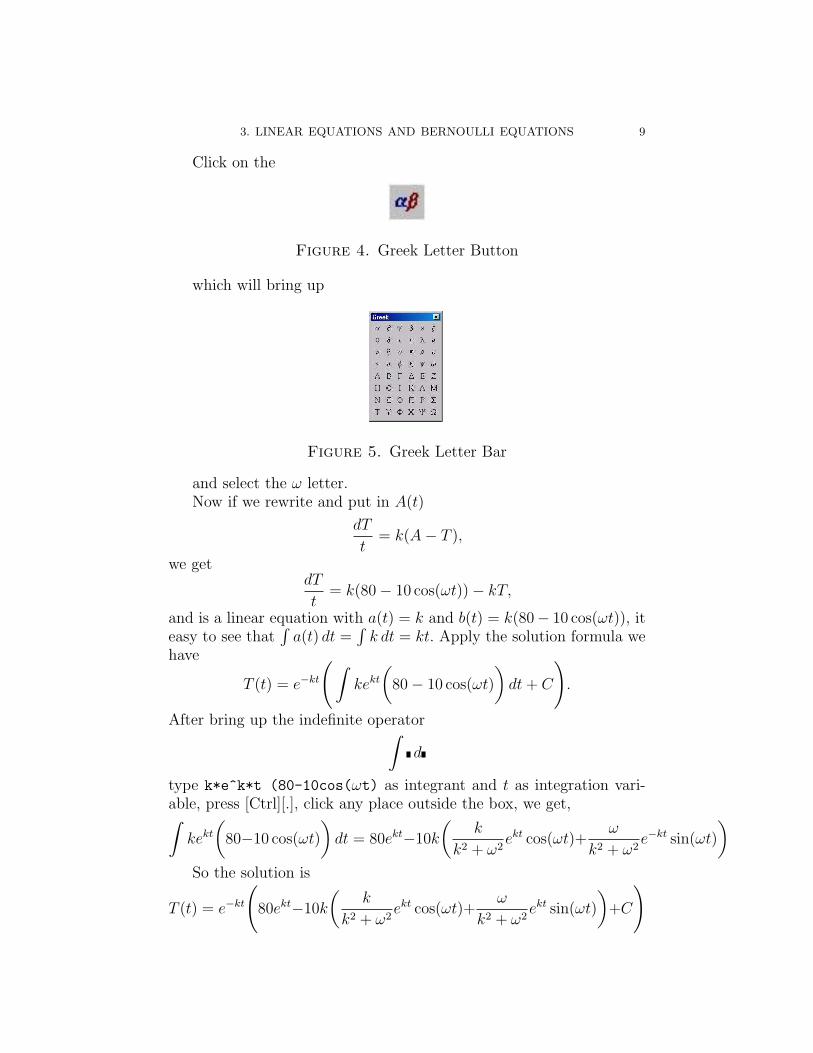
Example 3.2. If in Example 3.1, we set k = 0.2 and ω = π4, we

would have general solution

T (t) = e−0.2t

(80e0.2t−5

(3.2

0.64 + π2e0.2t cos(ωt)+

4π

0.64 + π2e0.2t sin(ωt)

)+C

)

The following graph displayed curves of several solutions with differentinitial values T (0).

Figure 6. Greek Letter Bar

The picture above exhibits the situation when the air condition failsat t = 0, so after a out 14 hours, the room temperature is the same asthe outside temperature!

Practice

(1) Find general solution to the following problem(a) y′ + 4xy = x2

(b) exy′ + exy = sin(x)(c) xy′ = 2y + x3 cos(x)

(d) y′ = 2xy + 3x2ex2

(e) (x2 + 4)y′ + 3xy = x

(f) (x2 + 1)y′ + 3x3y = 6xe−32x2

(2) Application: The equation y′ = ky models wide range ofnatural phenomena–any involving a quantity whose time rateof change is proportional to its current size.

Continuously Compounded Interest Rate: Let P (t)denote principle at time t, which will earn interest with rater(t) and compounded continuously, we have dP

dt= rP. Now


suppose r(t) = cos2(t), find the general solution and graphthe solution for several different value for the constant C inthe same coordinate. Explain the long time behavior of thesolutions.

Drug Elimination: Let A(t) be the amount of cer-tain drug in the bloodstream, measured by the excess over thenatural level of the drug. Then in many situations A(t) willdecline at a rate proportional to the current excess amount.That is

dA

dt= −λA,

where λ > 0 is called the elimination parameter of the drug.Suppose for one type of drug, λ(t) = 1

t2+4find the general

solution. Discuss its longtime behavior by graphing severalsolutions in the same coordinate.

3.2. Bernoulli Equations. A Bernoulli equation is an ODE ofthe form

dy

dx+ a(x)y = b(x)yn.(5)

You can see that when n = 1, we get linear equation. So linear equationis a special case of Bernoulli equation. On the other hand if we letv = y1−n, then

dv

dx= (1− n)y−n dy

dx

Dividing both side of (5) by yn, we have

y−n dy

dx+ a(x)y1−n = b(x)

So

1

1− n

dv

dx+ a(x)v = b(x).(6)

That is using the transformation v = y1−n, the Bernoulli equation fory becomes a linear equation for v.

Therefore to find the general solution for Bernoulli equation (5) wefirst find the general solution for the linear equation (6) of v, then using

y = v1

1−n to find y.


Example 3.3. In modelling a population with its births(per unittime) proportional to current population level and the deaths(per unittime) is proportional to the square of the current population, we have

dx

dt= ax− bx2

, which is called logistic differential equation. It is a Bernoulli equationwith n = 2 (Notice it is also a separable equation if a, b are constants.)

Solution Let v = x1−2 = x−1, then xv = 1 apply product rule ofdifferentiation, we have x′v + v′x = 0, plug in x′ = ax− bx2, we have

(ax− bx2)v + v′x = axv − bx2v + v′x = a− bx + v′x = 0 since xv = 1

So

a− bx + v′x = 0(7)

Divide (7) by x and notice 1x

is v, we have

v′ + av − b = 0,

or

v′ + av = b.

Apply the solution formula for linear equation we have

v = e−R

a dt

(∫beR

a dt dt + C

)

So

x =1

v=

eR

a dt

(∫

beR

a dt dt + C

)

a

Example 3.4. In the logistic model,

dx

dt= ax− bx2

, suppose a > 0, b > 0 are constants, we will discuss behavior of thesolutions.


Solution From Example 3.3,

x =eR

a dt

(∫

beR

a dt dt + C

)

So

x =eat

(∫

beat dt + C

) =eat

(baeat + C

) ,

is the general solution.When C = 0 we have x = a

b, a stead-state solution. Also, x = 0 is

another steady-state solution, which can’t be represented in the generalsolution.

We can rewrite x(t) as

x(t) =a

b + aCe−at,

since limt→∞ e−at = 0 So we have limt→∞ = ab. That is, as time goes

on the population will gradually settles itself at the level of ab. The

following picture shows that the solution curves approaches the liney = a

b= 10, with a = 0.2 and b = 0.002.

Figure 7. Population a = 0.2 and b = 0.02


Here is how to get the graph in Mathcad :

- we first defined a function x(t, C):= 0.20.02+Ce−0.2t with two argu-

ments t and C by typing x(t,C):0.2/0.02+C*e^-0.2t,- then we defined a range variable t:=0,0.1. . .20 by typingt:0,0.1;20,

- finally, type @ at a blank area to get the xy-plot; in the functionplace holder, we putx(t,0),x(t,-0.01),x(t,-0.008),x(t,0.004),x(t,0.01)

and type t in the variable place holder, and click at outside of thebox to get the graph.

a

4. Initial value problem and existence theorem

The problem of finding a particular solution x(t) of an ODE x′ =f(t, x) that satisfying condition x(t0) = x0 is called an initial valueproblem. The problem can be written{

x′ = f(t, x)x(t0) = x0

Since solving an ODE requires a lots of hard work, it is wise to know ifa given equation has any solution before march on the journey of finda solution. For the linear first order ODE x′+a(t)x = b(t) we followingexistence-uniqueness theorem.

Theorem 4.1. If the function a(t) and b(t) are continuous on theopen interval I containing the point t0, then the initial value problemx′+ a(t)x = b(t), x(t0) = x0 has a unique solution x(t) on I, givenby

x(t) = eR

a(t) dt

( ∫b(t)e−

Ra(t) dt dt + C

)(8)

with an appropriate value of C.

So solving an initial value problem for linear first order ODE is easy.One just apply the formula (8) and using the equation x(t0) = x0 tofind C.

Example 4.1. Solve the initial value problem x′+2tx = 4t3, x(0) =1.

Solution First we apply the formula (8)

x(t) = eR

a(t) dt

(∫b(t)e−

Ra(t) dt dt + C

),

4. INITIAL VALUE PROBLEM AND EXISTENCE THEOREM 15

with a(t) = 2t and b(t) = 4t3. So∫

a(t) dt =∫

2t dt = t2, and

x(t) = e−t2

(∫4t3et2 dt + C

).

Using method of substitution or Mathcad , we find

x(t) = e−t2(

2t2et2 − 2et2 + C

)

Let t = 0 we have x(0) = C− 2. From initial condition x(0) = 1 we seethat C = 3. So the solution is

x(t) = e−t2(

2t2et2 − 2et2 + 3

)

aHowever, for general first order ODE , the problem is not so nice,

the following theorem is a little bit hard to state and to understand.

Theorem 4.2. Let f(t, x) be defined on interval I. If the partial

derivative of f(t, x) with respect to y (denoted as ∂f(t,x)∂y

, reads ”par-

tial f(t,x) over partial y”) and f(t, x) are continuous at an open diskcentered at (t0, x0), then the initial value problem{

x′ = f(t, x)x(t0) = x0

has an unique solution on some open interval containing the point t0.

Remark 4.1. We will not discuss this existence and uniquenesstheorem for general ODE . But we would like to make some comments.

- To find ∂f(t,x)∂t

, you just need to treat x variable as a constant,

for example, let f(t, x) = t2x3 + 3t − 4x, we have ∂f(t,x)∂t

=2tx3+3, here 4x is a constant with respect to t, so the derivativeis 0, and x3 is also a constant, so t2x3 when taking derivativeagainst t we have 2tx3. Therefore finding partial derivative isas easy as to find ordinary derivative.

- This theorem only guarantees a solution defined for t in anopen interval, which might be a bounded interval. For examplex′ = x2, we see that x(t) = − 1

t+cis the general solution, if

c = −2 then the solution is only defined on interval (0, 2) asx(t) = − 1

t−2will become undefined at t = 2.

- Some time we could have more than one solution that satisfiesthe same initial condition, for example, for x′ = x

23 and x(0) =

0 we have two different solution, one is x(t) = 0 another one


is x(t) = t13 . The reason is that for f(t, x) = x

23 , ∂f(t,x)

∂x= 1

3√

x

which is undefined at (0, 0). So the conditions of the theoremare violated.

5. Phase and vector field diagrams

Sometimes it is more important to know the behavior of solutionsthan to know precisely detail of point-by-point of some particular so-lutions. Here we will discuss two diagrams to get an ”feel” of behaviorof solutions for a ODE without actually find any solution. The first,phase diagram, is used for the autonomous equations and is easy todraw. The second, vector field diagram, can be used for any equa-tion but harder to draw. These two diagrams make use of the facts:

(1) The derivative f ′(x) represent the slope of tangent line to thegraph y = f(x) at the point (x, f(x)).

(2) The sign of f ′(x) tell whether the graph is going up or down.If f ′(x) > 0 the graph is increasing.If f ′(x) < 0 the graph is going down.

(3) The second derivative f ′′(x) gives information about concav-ity:

If f ′′(x) > 0 the graph is concave upward.If f ′′(x) < 0 the graph is concave downward.

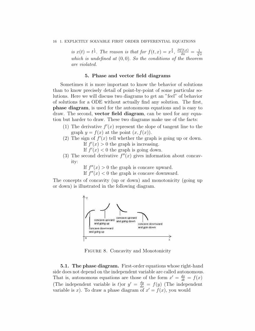
The concepts of concavity (up or down) and monotonicity (going upor down) is illustrated in the following diagram.

Figure 8. Concavity and Monotonicity

5.1. The phase diagram. First-order equations whose right-handside does not depend on the independent variable are called autonomous.That is, autonomous equations are those of the form x′ = dx

dt= f(x)

(The independent variable is t)or y′ = dydx

= f(y) (The independentvariable is x). To draw a phase diagram of x′ = f(x), you would

5. PHASE AND VECTOR FIELD DIAGRAMS 17

Step one: Set f(x) = 0 solve the equation. The solution is called thecritical number of the equation x′ = f(x).

Step two: Plot the solution one a horizontal (or vertical)number line.The solutions will divide the line into intervals (segments),pick any number from each interval (segment) and determinethe sign of the value of f(x) at the picked value.

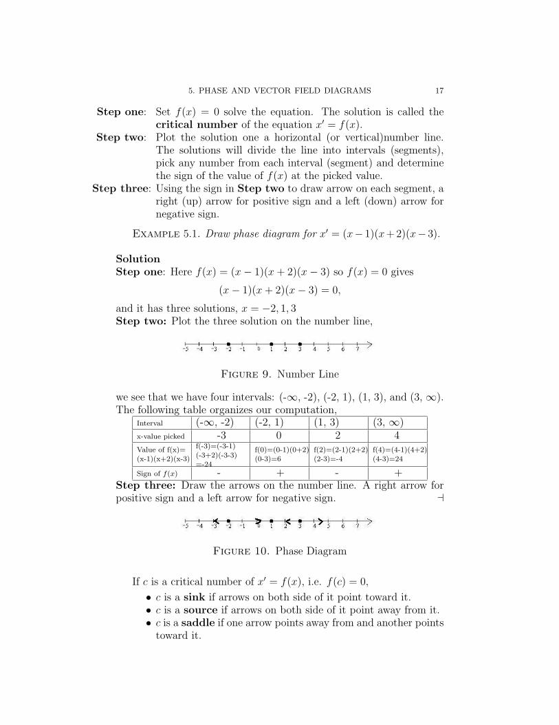
Step three: Using the sign in Step two to draw arrow on each segment, aright (up) arrow for positive sign and a left (down) arrow fornegative sign.

Example 5.1. Draw phase diagram for x′ = (x− 1)(x+2)(x− 3).

SolutionStep one: Here f(x) = (x− 1)(x + 2)(x− 3) so f(x) = 0 gives

(x− 1)(x + 2)(x− 3) = 0,

and it has three solutions, x = −2, 1, 3Step two: Plot the three solution on the number line,

Figure 9. Number Line

we see that we have four intervals: (-∞, -2), (-2, 1), (1, 3), and (3, ∞).The following table organizes our computation,

Interval (-∞, -2) (-2, 1) (1, 3) (3, ∞)x-value picked -3 0 2 4Value of f(x)=(x-1)(x+2)(x-3)

f(-3)=(-3-1)(-3+2)(-3-3)=-24

f(0)=(0-1)(0+2)(0-3)=6

f(2)=(2-1)(2+2)(2-3)=-4

f(4)=(4-1)(4+2)(4-3)=24

Sign of f(x) - + - +Step three: Draw the arrows on the number line. A right arrow forpositive sign and a left arrow for negative sign. a

Figure 10. Phase Diagram

If c is a critical number of x′ = f(x), i.e. f(c) = 0,

• c is a sink if arrows on both side of it point toward it.• c is a source if arrows on both side of it point away from it.• c is a saddle if one arrow points away from and another points

toward it.


In Example ??, c = 1 is a sink, c = −2, 3 are source.

From phase diagram and the sign of derivative of x′′ = df(x)dt

=df(x)dx

dxdt

= f(x)df(x)dx

, we can get an very good picture about the behaviorof the solutions.

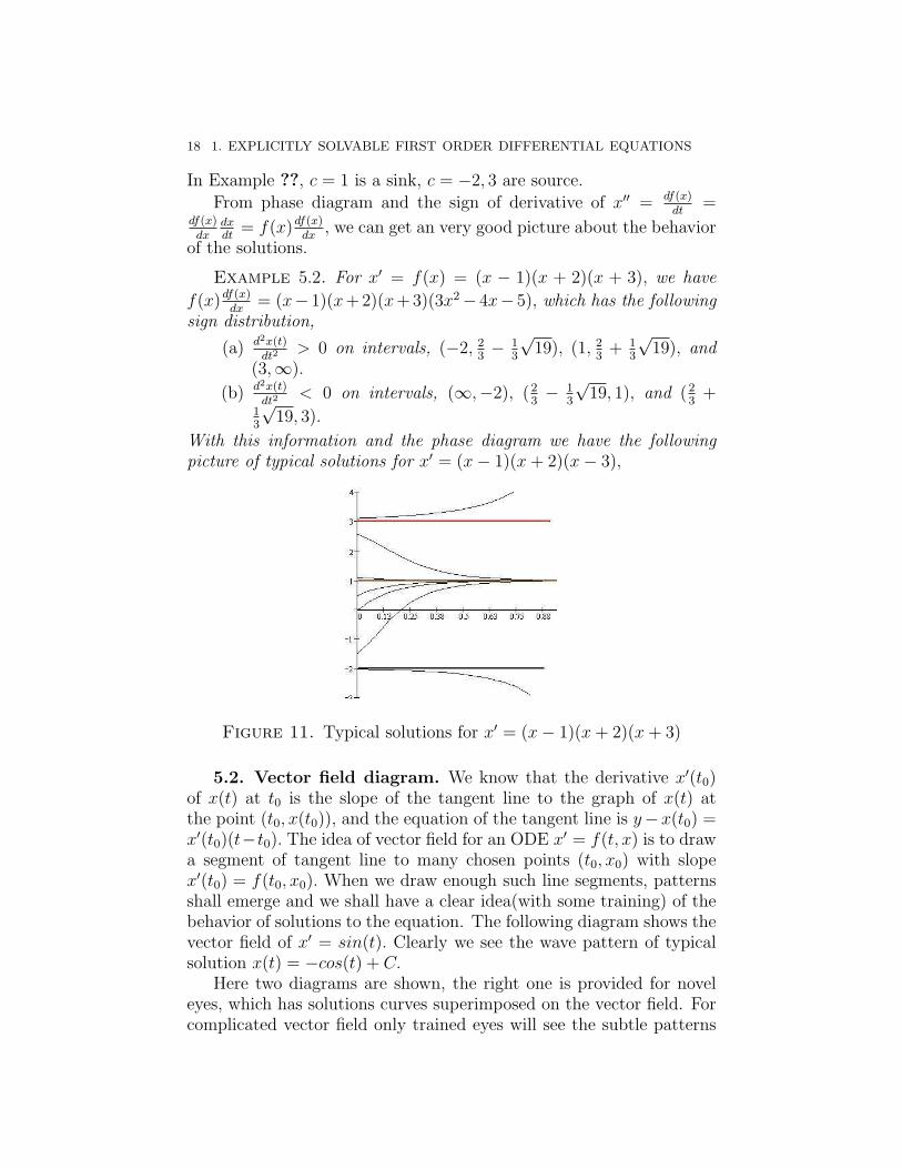
Example 5.2. For x′ = f(x) = (x − 1)(x + 2)(x + 3), we have

f(x)df(x)dx

= (x− 1)(x+2)(x+3)(3x2− 4x− 5), which has the followingsign distribution,

(a) d2x(t)dt2

> 0 on intervals, (−2, 23− 1

3

√19), (1, 2

3+ 1

3

√19), and

(3,∞).

(b) d2x(t)dt2

< 0 on intervals, (∞,−2), (23− 1

3

√19, 1), and (2

3+

13

√19, 3).

With this information and the phase diagram we have the followingpicture of typical solutions for x′ = (x− 1)(x + 2)(x− 3),

Figure 11. Typical solutions for x′ = (x− 1)(x + 2)(x + 3)

5.2. Vector field diagram. We know that the derivative x′(t0)of x(t) at t0 is the slope of the tangent line to the graph of x(t) atthe point (t0, x(t0)), and the equation of the tangent line is y−x(t0) =x′(t0)(t−t0). The idea of vector field for an ODE x′ = f(t, x) is to drawa segment of tangent line to many chosen points (t0, x0) with slopex′(t0) = f(t0, x0). When we draw enough such line segments, patternsshall emerge and we shall have a clear idea(with some training) of thebehavior of solutions to the equation. The following diagram shows thevector field of x′ = sin(t). Clearly we see the wave pattern of typicalsolution x(t) = −cos(t) + C.

Here two diagrams are shown, the right one is provided for noveleyes, which has solutions curves superimposed on the vector field. Forcomplicated vector field only trained eyes will see the subtle patterns


Figure 12. Vector field for f(t, x) = sin(t)

of the dynamics of solutions as shown in the next not so complicateddiagram,

Figure 13. Vector field for f(t, x) = t− x2

To graph the vector field diagram for y′ = f(x, y) by hand overrectangular region [a, b]× [c, d], you would do the following:

(1) Divide interval [a, b] into N equal length subintervals and [c,d] into M equal length subintervals, for [a, b] the length ish = b−a

Nand the subintervals are [a, a+h], [a+h, a+2h],· · · ;

for [c, d] the subinterval length is s = d−cM

and the subintervalsare [c, c+s], [c+s, c+2s], · · · .

(2) If we use xi = a + ih, i = 0, 1, · · · , N to denote the endingsof subintervals of [a, b] and yj = c + js, j = 0, 1, 2, · · · todenote the endings of subintervals of [c, d], then (xi, yj) formthe grid points, i = 0, 1, · · · , N ; j = 0, 1, · · · ,M. For eachpoint (xi, yj) compute the slope mij = f(xi, yj) and, from the


equation of tangent line y − yj = mij(x − xi) we get anotherpoint ((xi + h

2, yj + mij

h2).

(3) Draw line segment from (xi, yj) to ((xi + h, yj + mijh) for i =0, 1, · · · , N ; j = 0, 1, · · · , M.

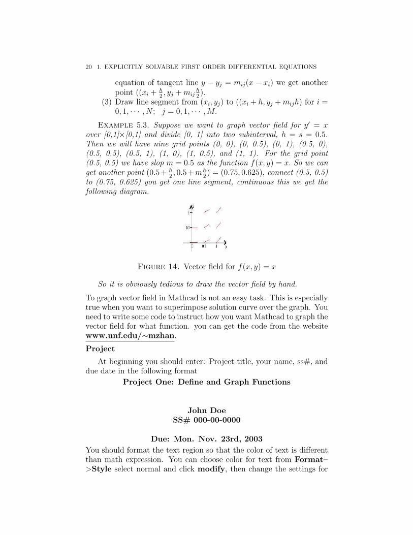
Example 5.3. Suppose we want to graph vector field for y′ = xover [0,1]×[0,1] and divide [0, 1] into two subinterval, h = s = 0.5.Then we will have nine grid points (0, 0), (0, 0.5), (0, 1), (0.5, 0),(0.5, 0.5), (0.5, 1), (1, 0), (1, 0.5), and (1, 1). For the grid point(0.5, 0.5) we have slop m = 0.5 as the function f(x, y) = x. So we canget another point (0.5+ h

2, 0.5+mh

2) = (0.75, 0.625), connect (0.5, 0.5)

to (0.75, 0.625) you get one line segment, continuous this we get thefollowing diagram.

Figure 14. Vector field for f(x, y) = x

So it is obviously tedious to draw the vector field by hand.

To graph vector field in Mathcad is not an easy task. This is especiallytrue when you want to superimpose solution curve over the graph. Youneed to write some code to instruct how you want Mathcad to graph thevector field for what function. you can get the code from the websitewww.unf.edu/∼mzhan.

Project

At beginning you should enter: Project title, your name, ss#, anddue date in the following format

Project One: Define and Graph Functions

John DoeSS# 000-00-0000

Due: Mon. Nov. 23rd, 2003

You should format the text region so that the color of text is differentthan math expression. You can choose color for text from Format–>Style select normal and click modify, then change the settings for


font. You can do this for headings etc. Graph Vector fieldGoal: Familiar your self with an many different kind of vector fields,defined by x′ = f(t, x), as possible and identify many general featuresof solutions, especially the following features,

• Does the equation has constant solutions? A constant solu-tion is shown in vector field as horizontal line segments sinceconstant solution has slope equals zero.

• Does solutions converge to an particular solution in the langrun?

• Do solutions grow to infinite an a finite time? Her vertical barsindicate a solution might become unbounded in short time.

• Do solutions display any periodicity? We know sin(t) has pe-riod of 2π and solution curve repeats itself. Here large intervalfor t might be needed.

You can use the following functions

• f(t, x) = sin(x)• f(t, x) = cos(t)• f(t, x) = x(x− 1)• f(t, x) = etx + sin(x)• f(t, x) = x + xsin(t)

You should use the provide Mathcad file at the websitewww.unf.edu/∼mzhan/vectorfield.mcdas a starting point and superimpose solutions to the vector fields sosupport your observation.

explicitly solvable first order diﬀerential equationsmzhan/chapter2.pdf · chapter 1 explicitly...

Documents