Solutions for Nonlinear Equations

Lecture 8

Alessandra Nardi

Thanks to Prof. Newton, Prof. Sangiovanni, Prof. White, Jaime Peraire, Deepak Ramaswamy, Michal Rewienski, and Karen Veroy

Last Lecture Review

• How to represent circuits– MNA– Voltage sources– How to assemble, X-stamp

• How to solve linear systems– Gaussian elimination– LU decomposition

Outline

• Nonlinear problems• Iterative Methods• Newton’s Method

– Derivation of Newton– Quadratic Convergence– Examples– Convergence Testing

• Multidimensonal Newton Method– Basic Algorithm – Quadratic convergence– Application to circuits

Need to Solve

( 1) 0d

t

VV

d sI I e

Nonlinear Problems - Example

0

1

IrI1 Id

0)1(1

0

11

1

1

IeIeR

III

tV

e

s

dr

11)( Ieg

Nonlinear Equations

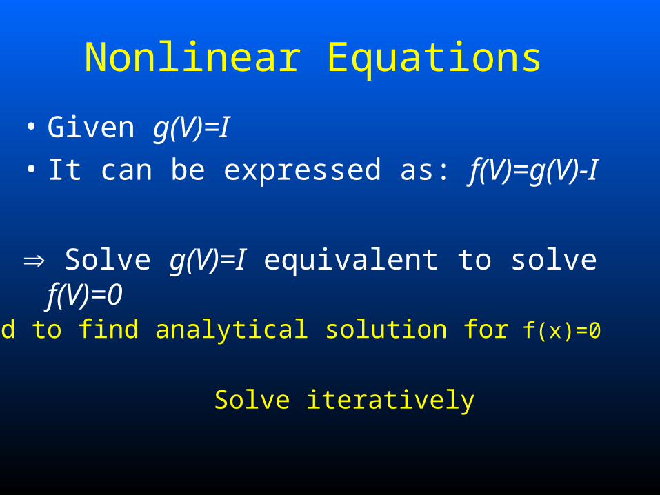
• Given g(V)=I

• It can be expressed as: f(V)=g(V)-I

Solve g(V)=I equivalent to solve f(V)=0

Hard to find analytical solution for f(x)=0

Solve iteratively

Nonlinear Equations – Iterative Methods

• Start from an initial value x0

• Generate a sequence of iterate xn-1, xn, xn+1 which hopefully converges to the solution x*

• Iterates are generated according to an iteration function F: xn+1=F(xn)

Ask• When does it converge to correct solution ?• What is the convergence rate ?

Newton-Raphson (NR) MethodConsists of linearizing the system.

Want to solve f(x)=0 Replace f(x) with its linearized version and solve.

Note: at each step need to evaluate f and f’

functionIterationxfxdx

dfxx

xxxdx

dfxfxf

iesTaylor Serxxxdx

dfxfxf

kkkk

kkkkk

)()(

))(()()(

))(()()(

11

11

***

Newton-Raphson Method – Graphical View

Newton-Raphson Method – Algorithm

Define iteration

Do k = 0 to ….

until convergence

• How about convergence?

• An iteration {x(k)} is said to converge with order q if there exists a vector norm such that for each k N:

qkk xxxx ˆˆ1

)()(1

1 kkkk xfxdx

dfxx

2* * * 2

2

*

0 ( ) ( ) ( )( ) ( )( )

some [ , ]

k k k k

k

df d ff x f x x x x x x x

dx dx

x x x

Mean Value theoremtruncates Taylor series

But10 ( ) ( )( )k k k kdf

f x x x xdx

by Newtondefinition

Newton-Raphson Method – Convergence

Subtracting

21 * 1 * 2

2 ( ) [ ( )] ( )( )k k kdf d f

x x x x x xdx d x

Convergence is quadratic

21 * * 2

2( )( ) ( )( )k k kdf d fx x x x x x

dx d x

Dividing through

21

2

21 * *

Let [ ( )] ( )

then

k k

k k k

df d fx x K

dx d x

x x K x x

Newton-Raphson Method – Convergence

Newton-Raphson Method – Convergence

Local Convergence Theorem

If

Then Newton’s method converges given a sufficiently close initial guess (and

convergence is quadratic)

boundedisK

boundeddx

fdb

roay from zebounded awdx

dfa

)

)

2

2

21

2 21 * * *

* 2

2

1 *

*

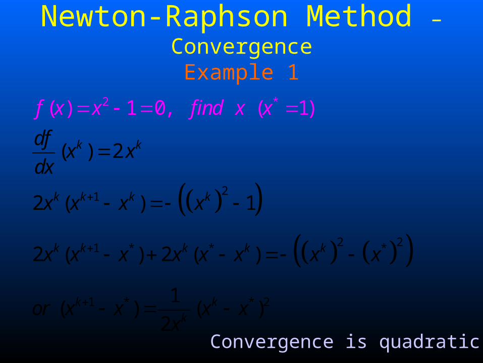
( ) 2

( ) 1 0,

2 ( ) 1

2 ( ) 2 ( )

1( ) (

( 1

)2

)

k k

k k k k

k k k k k

k kk

dfx x

dx

x x x x

x x x x x x x

f x x fin

x

d x x

or x x x xx

Convergence is quadratic

Newton-Raphson Method – ConvergenceExample 1

1 2

1 *

* *1

2 *

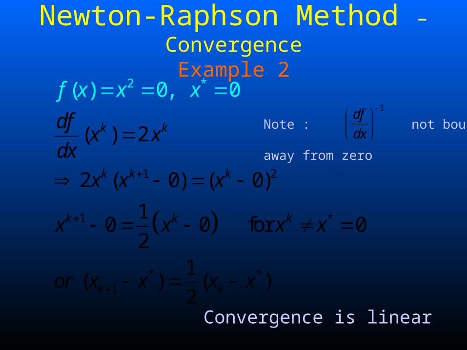
( ) 2

2 ( 0) ( 0)

10 0

( ) 0,

for 02

1( ) ( )

2

0

k k

k k k

k k k

k k

dfx x

dx

x x x

x x x x

or x x x

f x

x

x x

Convergence is linear

Note : not bounded

away from zero

1df

dx

Newton-Raphson Method – ConvergenceExample 2

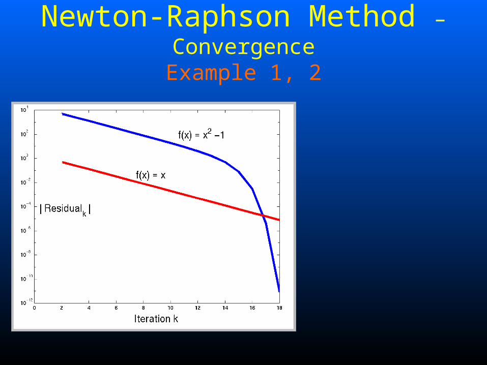
Newton-Raphson Method – ConvergenceExample 1, 2

0 Initial Guess,= 0x k

Repeat { 1

k

k k kf x

x x f xx

} Until ?

1 1? ?k k kf x thresholdx x threshold

1k k

Newton-Raphson Method – Convergence

Need a "delta-x" check to avoid false convergence

X

f(x)

1kx kx *x

1 a

kff x

1 1 a r

k k kx xx x x

Newton-Raphson Method – ConvergenceConvergence Checks

Also need an " " check to avoid false convergencef x

X

f(x)

1kx kx

*x

1 a

kff x

1 1 a r

k k kx xx x x

Newton-Raphson Method – ConvergenceConvergence Checks

demo2

Newton-Raphson Method – Convergence

X

f(x)

Convergence Depends on a Good Initial Guess

0x

1x2x 0x

1x

Newton-Raphson Method – ConvergenceLocal Convergence

Convergence Depends on a Good Initial Guess

Newton-Raphson Method – ConvergenceLocal Convergence

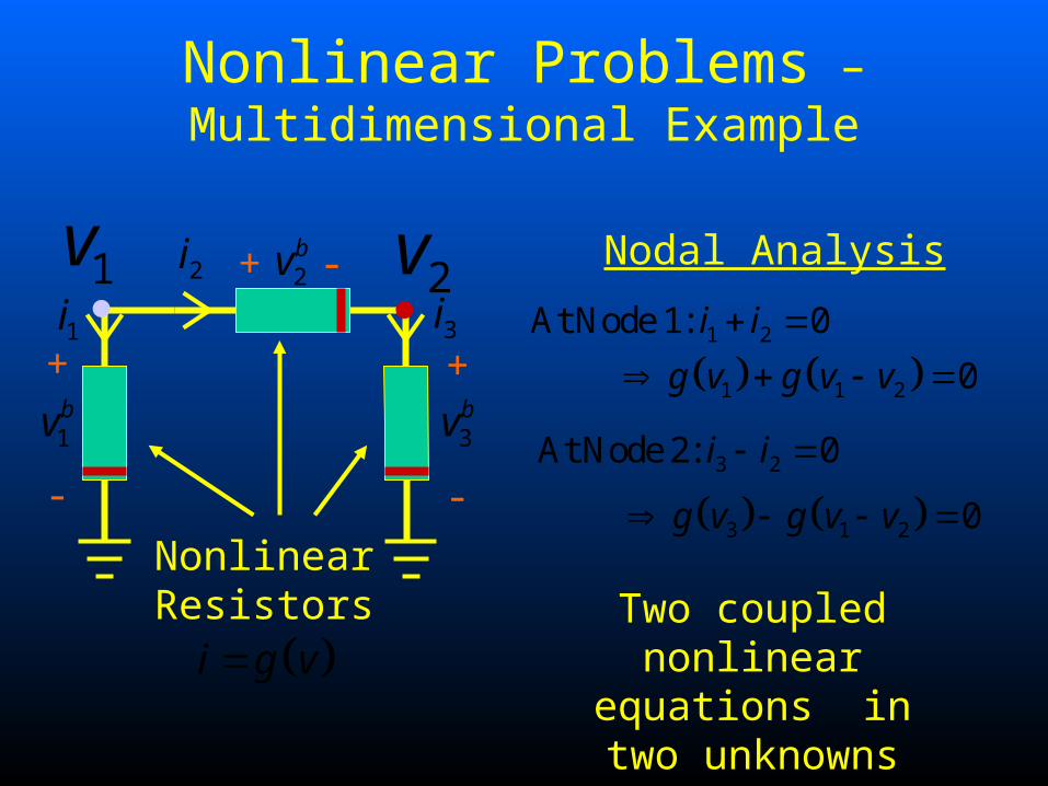
Nodal Analysis

1 2At Node 1: 0i i

1bv

+

-

1i2i 2

bv

3i+ -

3bv

+

-

NonlinearResistors

i g v

1v2v

1 1 2 0g v g v v

3 2At Node 2: 0i i

3 1 2 0g v g v v

Two coupled nonlinear equations in two unknowns

Nonlinear Problems – Multidimensional Example

* *Problem: Find such tha 0t x F x * N N N and : x F

Multidimensional Newton Method

functionIterationxFxJxx

atrixJacobian M

x

xF

x

xF

x

xF

x

xF

xJ

iesTaylor SerxxxJxFxF

kkkk

N

NN

N

)()(

)()(

)()(

)(

))(()()(

11

1

1

1

1

***

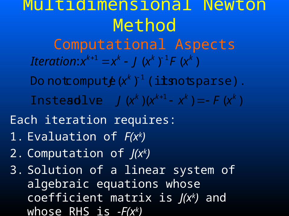
Multidimensional Newton MethodComputational Aspects

)()()( :solve Instead

sparse).not is(it )( computenot Do

)()(:

1

1

11

kkkk

k

kkkk

xFxxxJ

xJ

xFxJxxIteration

Each iteration requires:

1. Evaluation of F(xk)

2. Computation of J(xk)

3. Solution of a linear system of algebraic equations whose coefficient matrix is J(xk) and whose RHS is -F(xk)

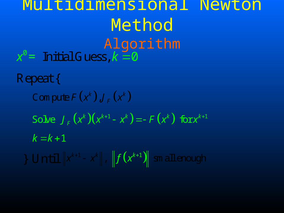
0 Initial Guess,= 0x k

Repeat {

1 1Solve for k k k k kFJ x x x F x x

} Until 11 , small en ug o hkk kx x f x

1k k

Compute ,k kFF x J x

Multidimensional Newton MethodAlgorithm

If

1) Inverse is boundedkFa J x

) Derivative is Lipschitz ContF Fb J x J y x y

Then Newton’s method converges given a sufficiently close initial guess (and

convergence is quadratic)

Multidimensional Newton Method Convergence

Local Convergence Theorem

Application of NR to Circuit Equations

0

1

IrI1 Id

01

,

0

1

11

1

11

11

1

1

11

1

1

1

11

k

dk

k

k

k

v

kk

r

VV

S

I

VV

Sk

k

VV

S

kkkkk

VVeV

I

RIeI

R

VVf

eIVgIVgR

VVf

VVVfVfVf

Note: G0 and Id depend on the iteration count k G0=G0(k) and Id=Id(k)

Application of NR to Circuit EquationsCompanion Network – MNA templates

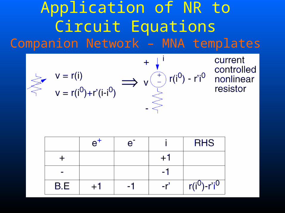
Application of NR to Circuit EquationsCompanion Network – MNA templates

Modeling a MOSFET(MOS Level 1, linear regime)

d

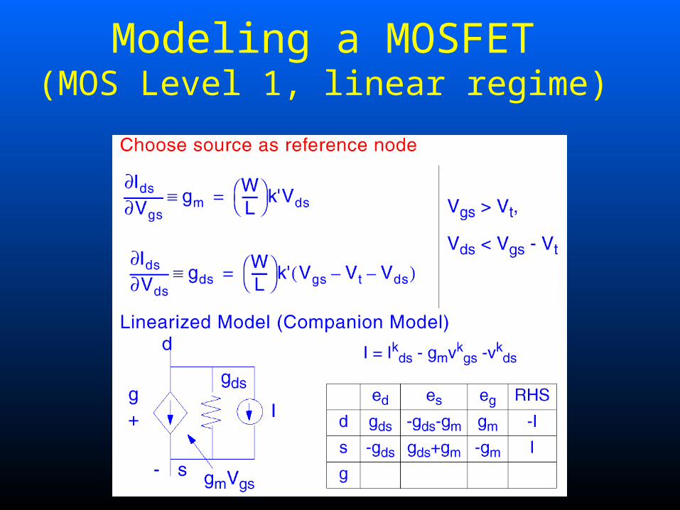
Modeling a MOSFET(MOS Level 1, linear regime)

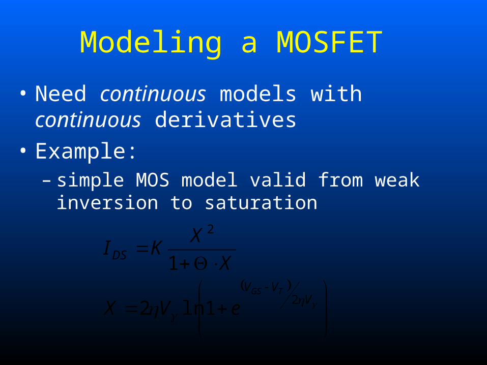
Modeling a MOSFET

• Need continuous models with continuous derivatives

• Example: – simple MOS model valid from weak inversion to

saturation

VVV

DS

TGS

eVX

X

XKI

2

2

1ln2

1

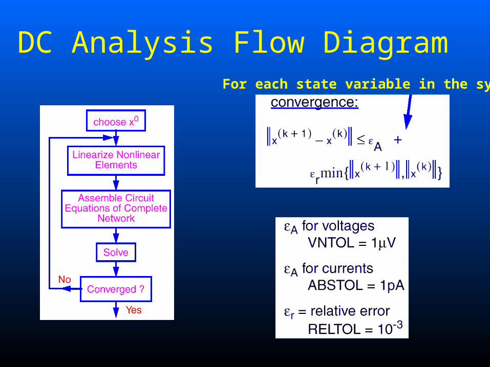
DC Analysis Flow DiagramFor each state variable in the system

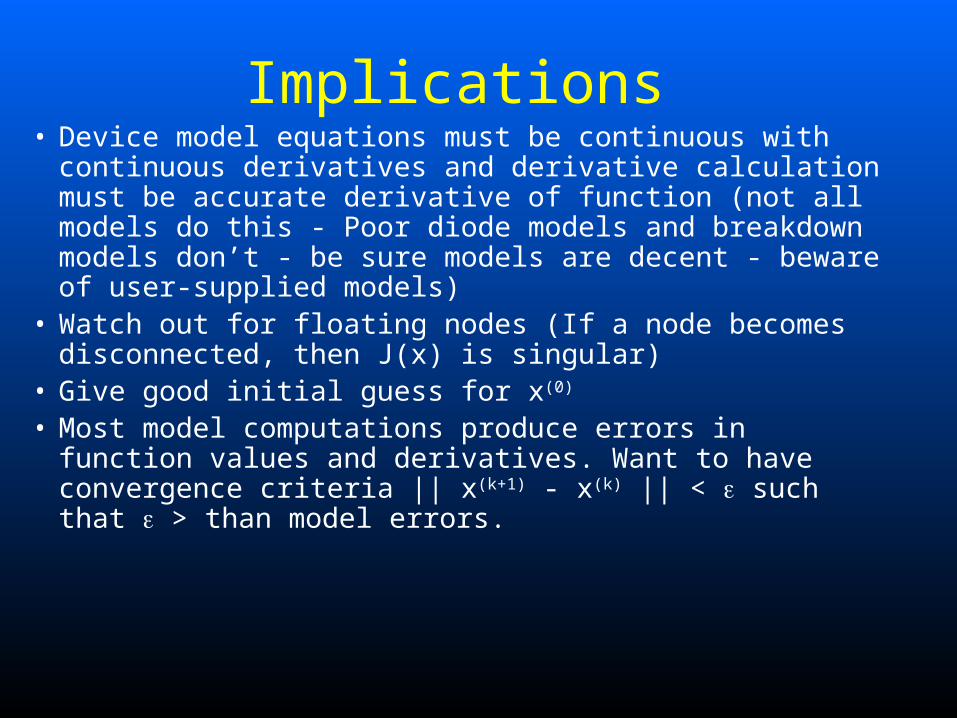
Implications• Device model equations must be continuous with continuous

derivatives and derivative calculation must be accurate derivative of function (not all models do this - Poor diode models and breakdown models don’t - be sure models are decent - beware of user-supplied models)

• Watch out for floating nodes (If a node becomes disconnected, then J(x) is singular)

• Give good initial guess for x(0)

• Most model computations produce errors in function values and derivatives. Want to have convergence criteria || x(k+1) - x(k) || < such that > than model errors.

Summary

• Nonlinear problems

• Iterative Methods

• Newton’s Method– Derivation of Newton

– Quadratic Convergence

– Examples

– Convergence Testing

• Multidimensional Newton Method– Basic Algorithm

– Quadratic convergence

– Application to circuits

Methods for Ordinary Differential Equations

Lecture 10

Alessandra Nardi

Thanks to Prof. Jacob White, Deepak Ramaswamy Jaime Peraire, Michal Rewienski, and Karen Veroy

Outline

• Transient Analysis of dynamical circuits– i.e., circuits containing C and/or L

• Examples

• Solution of Ordinary Differential Equations (Initial Value Problems – IVP)– Forward Euler (FE), Backward Euler (BE) and

Trapezoidal Rule (TR)– Multistep methods– Convergence

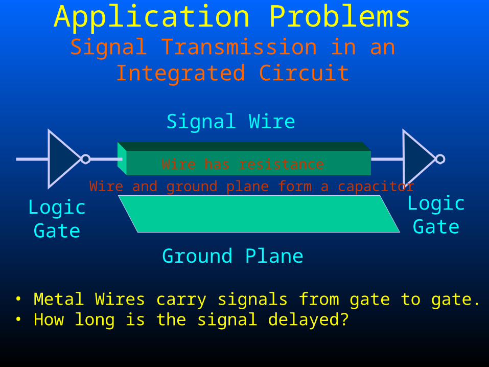
Ground Plane

Signal Wire

LogicGate

LogicGate

• Metal Wires carry signals from gate to gate.• How long is the signal delayed?

Wire and ground plane form a capacitor

Wire has resistance

Application ProblemsSignal Transmission in an Integrated Circuit

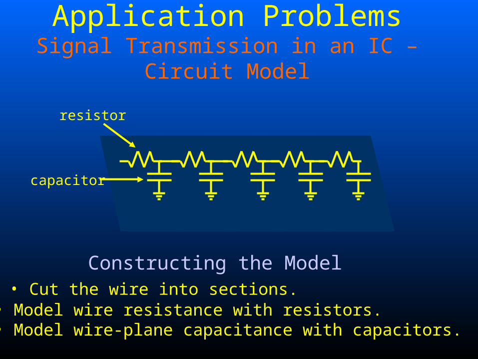
capacitor

resistor

• Model wire resistance with resistors.• Model wire-plane capacitance with capacitors.

Constructing the Model• Cut the wire into sections.

Application ProblemsSignal Transmission in an IC – Circuit Model

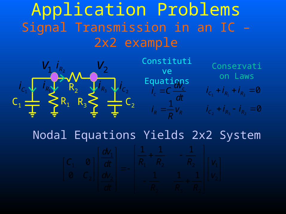
Nodal Equations Yields 2x2 System

C1

R2

R1 R3 C2

Constitutive Equations

cc

dvi C

dt

1R Ri v

R

Conservation Laws

1 1 20C R Ri i i

2 3 20C R Ri i i

1

1 2 21 1

2 22

2 3 2

1 1 1

0

0 1 1 1

dvR R RC vdt

C vdv

R R Rdt

1Ri1Ci

2Ri

2Ci3Ri

1v 2v

Application ProblemsSignal Transmission in an IC – 2x2 example

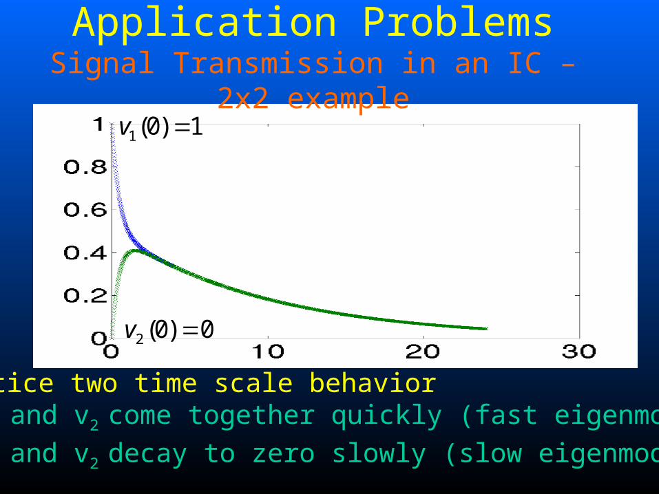
1(0) 1v

2 (0) 0v

Notice two time scale behavior• v1 and v2 come together quickly (fast eigenmode).• v1 and v2 decay to zero slowly (slow eigenmode).

Application ProblemsSignal Transmission in an IC – 2x2 example

Circuit Equation Formulation

• For dynamical circuits equations can be written compactly:

• For sake of simplicity, we shall discuss first order ODEs in the form:

riablescircuit va of vector theis where

)0(

0),,)(

(

0

x

xx

txdt

tdxF

),()(

txfdt

tdx

Ordinary Differential EquationsInitial Value Problems (IVP)

Typically analytic solutions are not available

solve it numerically

.condition initial given the intervalan in

)(

),()(

:(IVP) Problem Value Initial Solve

00

00

x,T][t

xtx

txfdt

tdx

• Not necessarily a solution exists and is unique for:

• It turns out that, under rather mild conditions on the continuity and differentiability of F, it can be proven that there exists a unique solution.

• Also, for sake of simplicity only consider

linear case:

0),,( tydt

dyF

We shall assume that has a unique solution 0),,( tydt

dyF

00 )(

)()(

xtx

tAxdt

tdx

Ordinary Differential Equations Assumptions and Simplifications

First - Discretize Time

Second - Represent x(t) using values at ti

ˆ ( )llx x t

Approx. sol’n

Exact sol’n

Third - Approximate using the discrete ( )l

dx t

dtˆ 'slx

1 1

1

ˆ ˆ ˆ ˆExample: ( )

l l l l

ll l

d x x x xx t or

dt t t

Lt T1t 2t 1Lt 0

t t t

1t 2t 3t Lt0

3x̂ 4x̂1x̂

2x̂

Finite Difference MethodsBasic Concepts

lt 1lt t

x

1( ) ( )slope l lx t x t

t

slope ( )l

dx t

dt

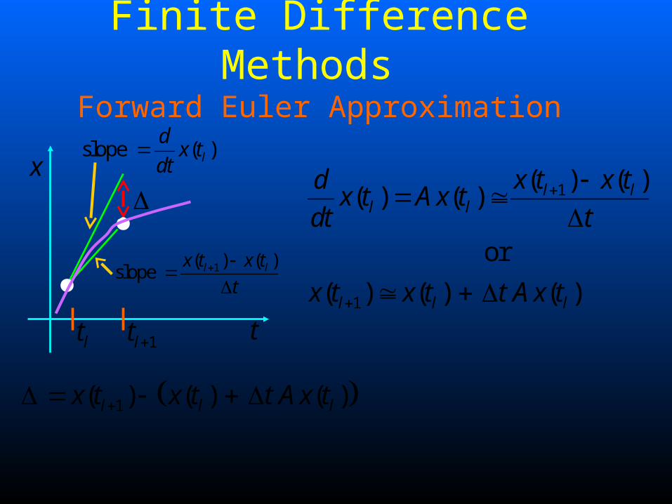
1( ) ( ) ( )l l lx t x t t A x t

1

1

( ) ( )( ) ( )

or

( ) ( ) ( )

l ll l

l l l

x t x tdx t A x t

dt t

x t x t t A x t

Finite Difference Methods Forward Euler Approximation

1t 2t t

x

(0)tAx

11 ˆ( ) (0) 0x t x x tAx

3t

2 1 12 ˆ ˆ ˆ( )x t x x tAx

1ˆtAx

1 1ˆ ˆ ˆ( ) L L LLx t x x tAx

Finite Difference Methods Forward Euler Algorithm

lt 1lt t

x 1slope ( )l

dx t

dt

1( ) ( )slope l lx t x t

t

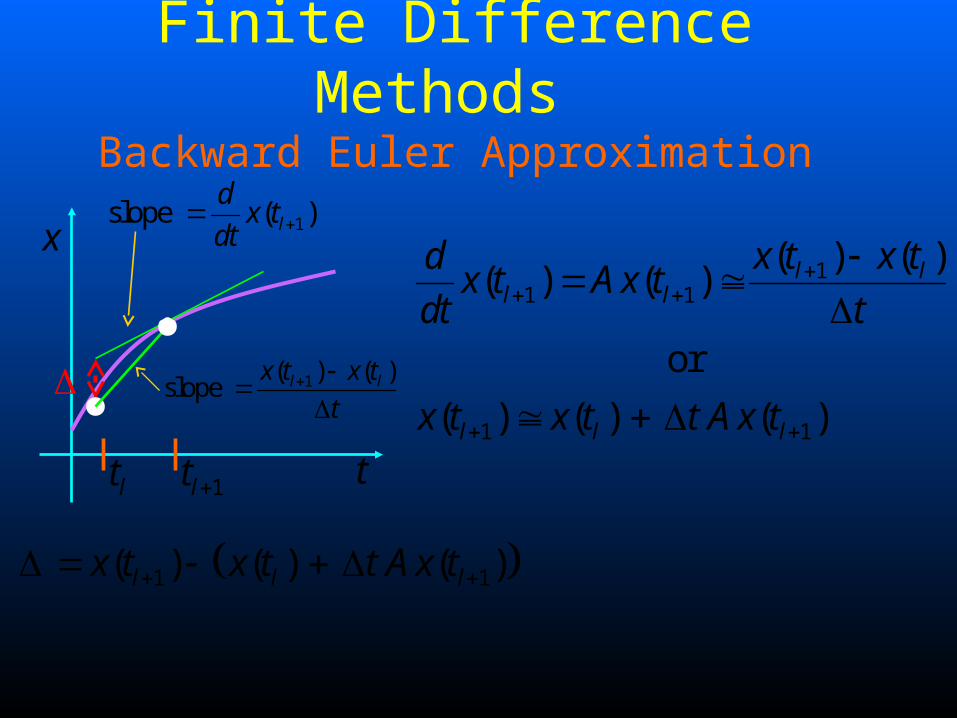
1 1( ) ( ) ( )l l lx t x t t A x t

11 1

1 1

( ) ( )( ) ( )

or

( ) ( ) ( )

l ll l

l l l

x t x tdx t A x t

dt t

x t x t t A x t

Finite Difference Methods Backward Euler Approximation

1t 2t t

x

1ˆtAx

2ˆtAx

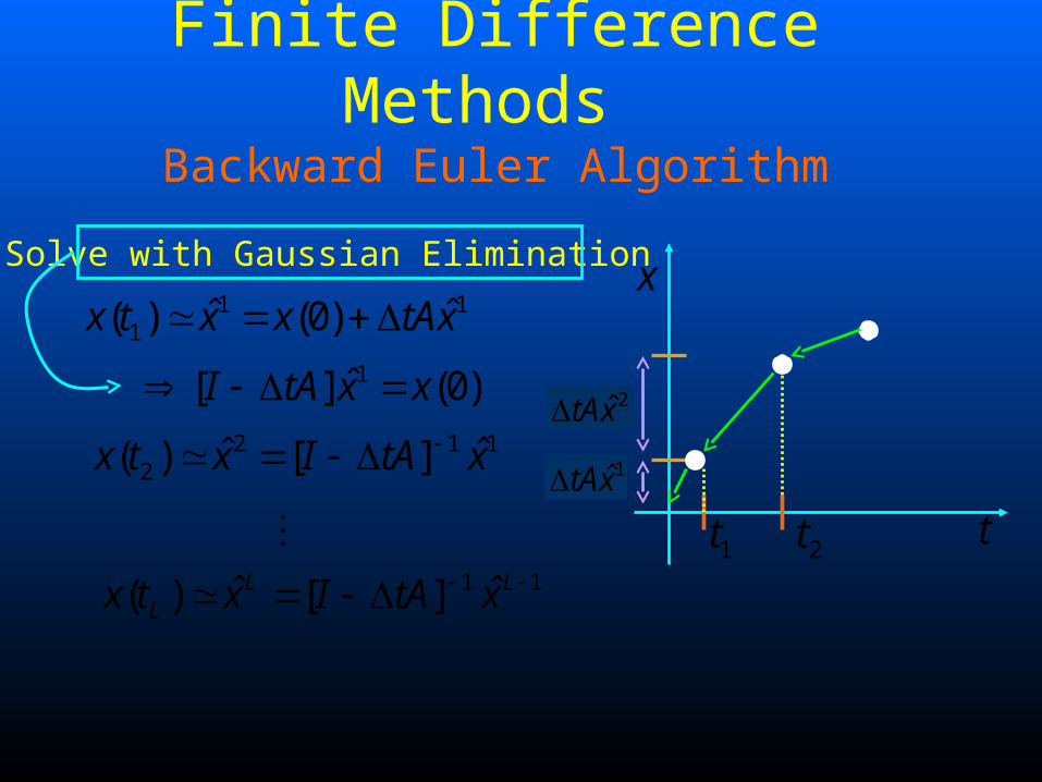
1 11 ˆ ˆ( ) (0)x t x x tAx

Solve with Gaussian Elimination

1ˆ[ ] (0)I tA x x

1 1ˆ ˆ( ) [ ]L LLx t x I tA x

2 1 12 ˆ ˆ( ) [ ]x t x I tA x

Finite Difference Methods Backward Euler Algorithm

1

1

1

1 1

1( ( ) ( ))

21

( ( ) ( ))2

( ) ( )

1( ) ( ) ( ( ) ( ))

2

l l

l l

l l

l l l l

d dx t x t

dt dt

Ax t Ax t

x t x t

t

x t x t tA x t x t

t

x

1( ) ( )slope l lx t x t

t

slope ( )l

dx t

dt

1slope ( )l

dx t

dt

1 1

1 1( ( ) ( )) ( ( ) ( ))

2 2l l l lx t tAx t x t tAx t

Finite Difference Methods Trapezoidal Rule Approximation

1t 2t t

x

1ˆ (0)2 2

t tI A x I A x

Solve with Gaussian Elimination

1 11 ˆ ˆ( ) (0) (0)

2

tx t x x Ax Ax

12 1

2

11

ˆ ˆ( )2 2

ˆ ˆ( )2 2

L LL

t tx t x I A I A x

t tx t x I A I A x

Finite Difference Methods Trapezoidal Rule Algorithm

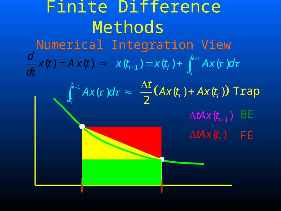
1

1( ) (( ) )) )( (l

l

t

l l t

dx t x t x t A dx t xA

dt

lt 1lt

1

( )l

l

t

tAx d

1( )ltAx t BE

( )ltAx t FE

( ) ( )2 l l

tAx t Ax t

Trap

Finite Difference Methods Numerical Integration View

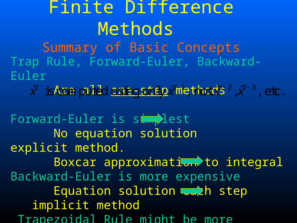
Trap Rule, Forward-Euler, Backward-Euler Are all one-step methods

Forward-Euler is simplest No equation solution explicit method. Boxcar approximation to integralBackward-Euler is more expensive Equation solution each step implicit method Trapezoidal Rule might be more accurate

Equation solution each step implicit method

Trapezoidal approximation to integral

1 2 3ˆ ˆ ˆ ˆ is computed using only , not , , etc.l l l lx x x x

Finite Difference Methods Summary of Basic Concepts

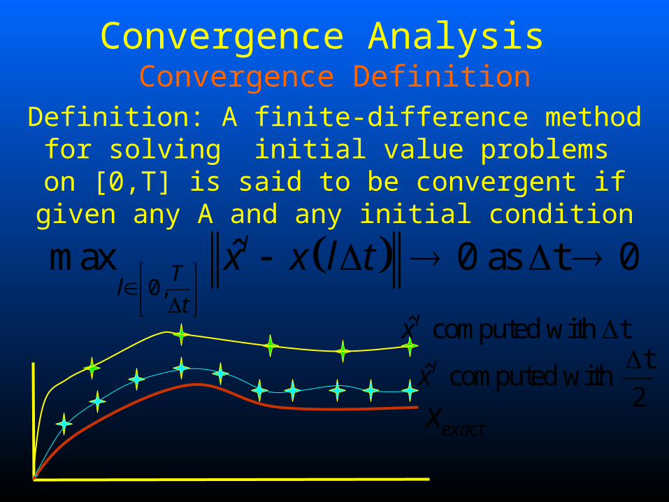
Definition: A finite-difference method for solving initial value problems on [0,T] is said to be

convergent if given any A and any initial condition

0,

ˆmax 0 as t 0lT

lt

x x l t

exactx

tˆ computed with

2lx

ˆ computed with tlx

Convergence Analysis Convergence Definition

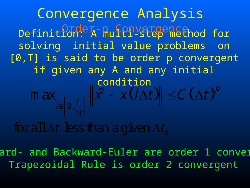
Definition: A multi-step method for solving initial value problems on [0,T] is said to be order p

convergent if given any A and any initial condition

0,

ˆmaxpl

Tl

t

x x l t C t

0for all less than a given t t

Forward- and Backward-Euler are order 1 convergentTrapezoidal Rule is order 2 convergent

Convergence Analysis Order-p Convergence

Multistep Methods – Convergence Analysis

Two types of error

made.been haserror previous no assuming ,solution theof value

exact theand ˆ valuecomputed ebetween th difference theis

at methodn integratioan of (LTE)Error Truncation Local The

1

1

1

)x(t

x

t

l

l

l

exactly.known iscondition

initial only the that assuming ,solution theof value

exact theand ˆ valuecomputed ebetween th difference theis

at methodn integratioan of (GTE)Error Truncation Global The

1

1

1

)x(t

x

t

l

l

l

• For convergence we need to look at max error over the whole time interval [0,T]– We look at GTE

• Not enough to look at LTE, in fact:– As I take smaller and smaller timesteps t, I would

like my solution to approach exact solution better and better over the whole time interval, even though I have to add up LTE from more timesteps.

Multistep Methods – Convergence Analysis

Two conditions for Convergence

1) Local Condition: One step errors are small (consistency)

2) Global Condition: The single step errors do not grow too quickly (stability)

Typically verified using Taylor Series

All one-step methods are stable in this sense.

Multistep Methods – Convergence Analysis

Two conditions for Convergence

Definition: A one-step method for solving initial value problems on an interval [0,T] is said to be consistent if for any A and any initial condition

1ˆ0 as t 0

x x t

t

One-step Methods – Convergence Analysis

Consistency definition

Forward-Euler definition

22

2

0()

2 0

dxtdxxtxt

dtdt

Expanding in about zero yields t

1ˆ00 xxtAx

Noting that (0)(0) and subtractingd

xAxdt

22

12 ˆ

2

tdxxxt

dt

Proves the theorem if

derivatives of x are bounded

0,t

One-step Methods – Convergence Analysis

Consistency for Forward Euler

Forward-Euler definition

1l

xltxlttAxlte

Expanding in about yields tlt 1

ˆˆ ˆlll

xxtAx

where is the "one-step" error bounded byl

e

2

2

[0,]2 , where 0.5maxl

T

dxeCtC

dt

One-step Methods – Convergence Analysis

Convergence Analysis for Forward Euler

ˆ Define the "Global" errorll

Exxlt

1ˆˆ 1

lllxxltItAxxlte

Subtracting the previous slide equations

Taking norms and using the bound on l

e

1 lllEItAEe

2 1

21

ll

l

EItAECt

tAECt

One-step Methods – Convergence Analysis

Convergence Analysis for Forward Euler

Example

+-

I1

R

C

V2

VS

V1

SVV

IVR

VR

VRdt

dVCV

R

2

121

21

1

011

011

Sk

kkk

kk

kk

Sk

kkk

kkk

k

VV

IVR

VR

t

VCV

Rt

VCV

R

VV

IVR

VR

VRt

VVCV

R

21

11

21

11

12

1

111

1

21

11

21

11

21

1111

1

011

11

011

011

BE

Sk

kkk

kk

kk

Sk

kkk

kkk

k

VV

IVR

VR

VRt

VCV

Rt

VC

VV

IVR

VR

VRt

VVCV

R

2

121

21

11

1

2

121

211

11

011

11

011

011

FE

Conclusions

• Introduced basic non-linear equation solution techniques– How to get good initial points?– Is it efficient?

• Introduced basic differential eqns solution techniques– Stability?– How to choose time-step– Stiffness– Other methods?