solutions. copyright © houghton mifflin company.all rights reserved. presentation of lecture...
TRANSCRIPT
Solutions

Copyright © Houghton Mifflin Company.All rights reserved. Presentation of Lecture Outlines, 12–2
– A colloid, although it also appears to be homogeneous, consists of comparatively large particles of a substance dispersed throughout another substance.
– In this chapter, we will examine the properties of each of these systems.
Solution Formation
• A solution is a homogeneous mixture of two or more substances, consisting of ions or molecules. (See Animation: Solution Equilibrium).
Copyright © Houghton Mifflin Company.All rights reserved. Presentation of Lecture Outlines, 12–3
Types of Solutions
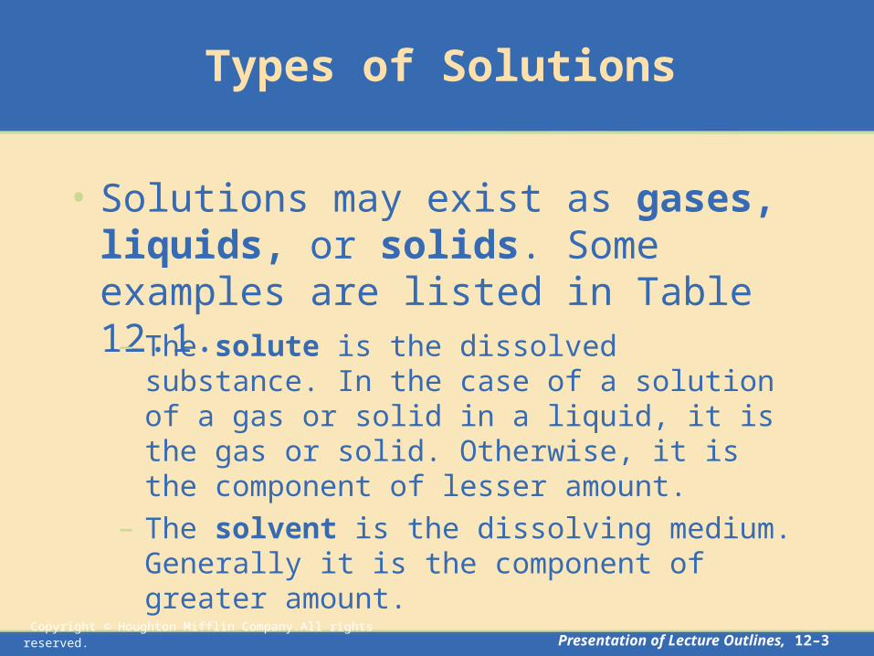
• Solutions may exist as gases, liquids, or solids. Some examples are listed in Table 12.1.
– The solute is the dissolved substance. In the case of a solution of a gas or solid in a liquid, it is the gas or solid. Otherwise, it is the component of lesser amount.
– The solvent is the dissolving medium. Generally it is the component of greater amount.

Copyright © Houghton Mifflin Company.All rights reserved. Presentation of Lecture Outlines, 12–4
Gaseous Solutions
• Nonreactive gases can mix in all proportions to give a gaseous solution.
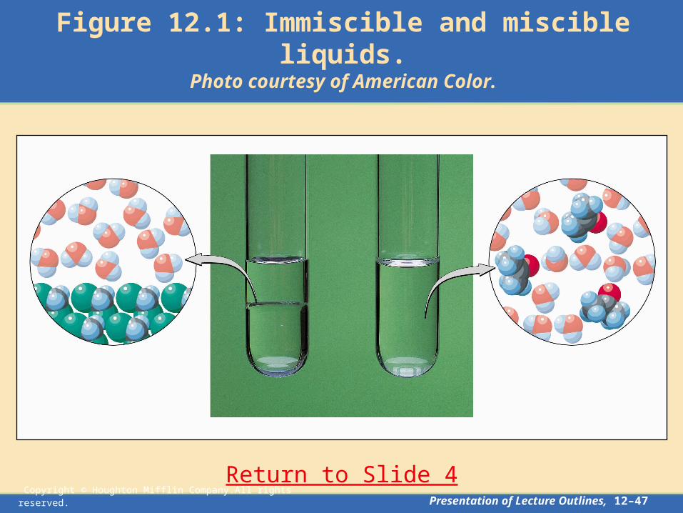
– Fluids that dissolve in each other in all proportions are said to be miscible fluids.
– If two fluids do not mix, they are said to be immiscible. (See Figure 12.1)
– For example, air is a solution of oxygen, nitrogen, and smaller amounts of other gases.

Copyright © Houghton Mifflin Company.All rights reserved. Presentation of Lecture Outlines, 12–5
Liquid Solutions
• Liquid solutions are the most common types of solutions found in the chemistry lab.
– Many inorganic compounds are soluble in water or other suitable solvents.
– Rates of chemical reactions increase when the likelihood of molecular collisions increases.
– This increase in molecular collisions is enhanced when molecules move freely in solution.
(See Animation: Dissolution of a Solid in a Liquid)
Copyright © Houghton Mifflin Company.All rights reserved. Presentation of Lecture Outlines, 12–6
Solid Solutions
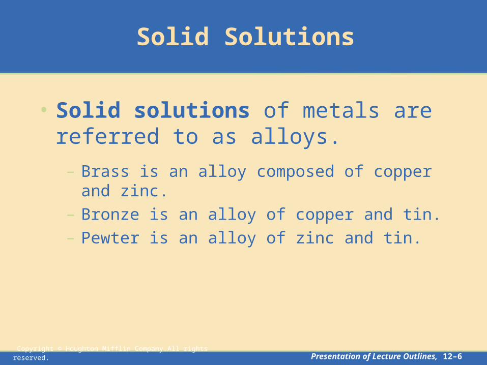
• Solid solutions of metals are referred to as alloys.
– Brass is an alloy composed of copper and zinc.– Bronze is an alloy of copper and tin.– Pewter is an alloy of zinc and tin.
Copyright © Houghton Mifflin Company.All rights reserved. Presentation of Lecture Outlines, 12–7
Solubility and the Solution Process
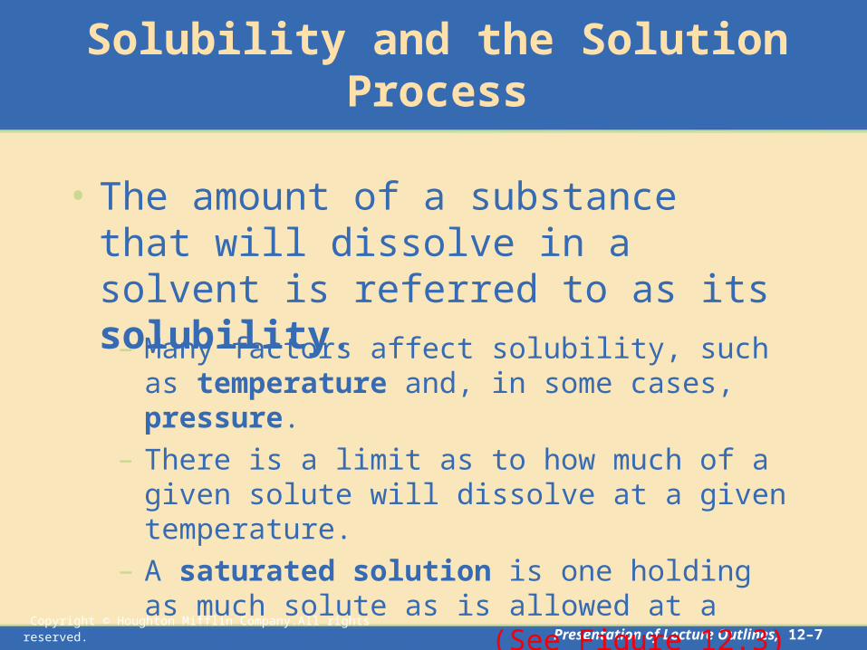
• The amount of a substance that will dissolve in a solvent is referred to as its solubility.
– Many factors affect solubility, such as temperature and, in some cases, pressure.
– There is a limit as to how much of a given solute will dissolve at a given temperature.
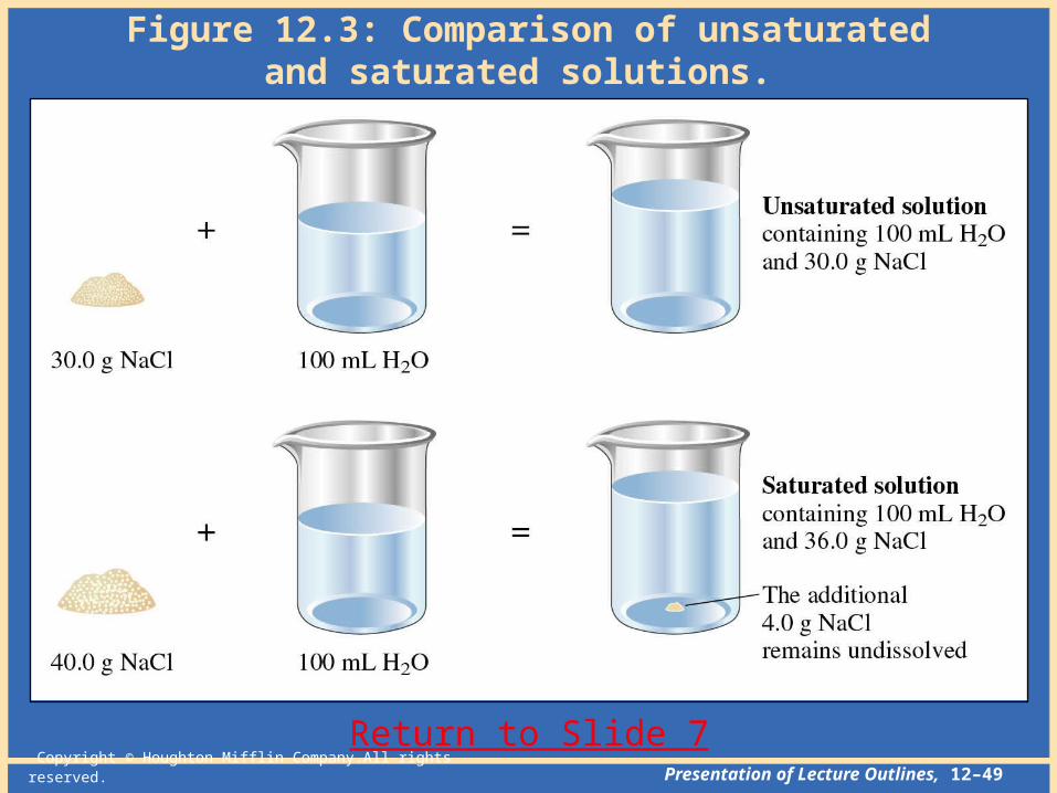
– A saturated solution is one holding as much solute as is allowed at a stated temperature. (See Figure 12.3)

Copyright © Houghton Mifflin Company.All rights reserved. Presentation of Lecture Outlines, 12–8
Solubility: Saturated Solutions
• Sometimes it is possible to obtain a supersaturated solution, that is, one that contains more solute than is allowed at a given temperature.
– Supersaturated solutions are unstable.– If a small crystal of the solute is added to a
supersaturated solution, the excess immediately crystallizes out (See Figure 12.4).

Copyright © Houghton Mifflin Company.All rights reserved. Presentation of Lecture Outlines, 12–9
Factors in Explaining Solubility
• In most cases, “like dissolves like.”
– This means that polar solvents dissolve polar (or ionic) solutes and nonpolar solvents dissolve nonpolar solutes.
– The relative force of attraction of the solute for the solvent is a major factor in their solubility.
Copyright © Houghton Mifflin Company.All rights reserved. Presentation of Lecture Outlines, 12–10
Molecular Solutions
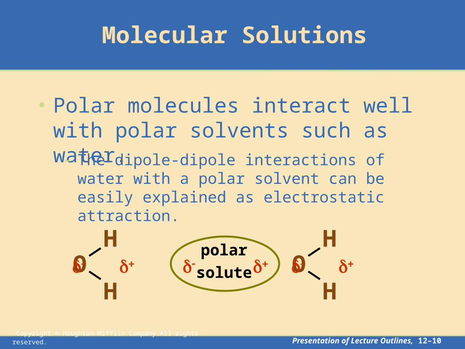
• Polar molecules interact well with polar solvents such as water.
– The dipole-dipole interactions of water with a polar solvent can be easily explained as electrostatic attraction.
polar
solute
HO
H
HO
H
Copyright © Houghton Mifflin Company.All rights reserved. Presentation of Lecture Outlines, 12–11
Molecular Solutions
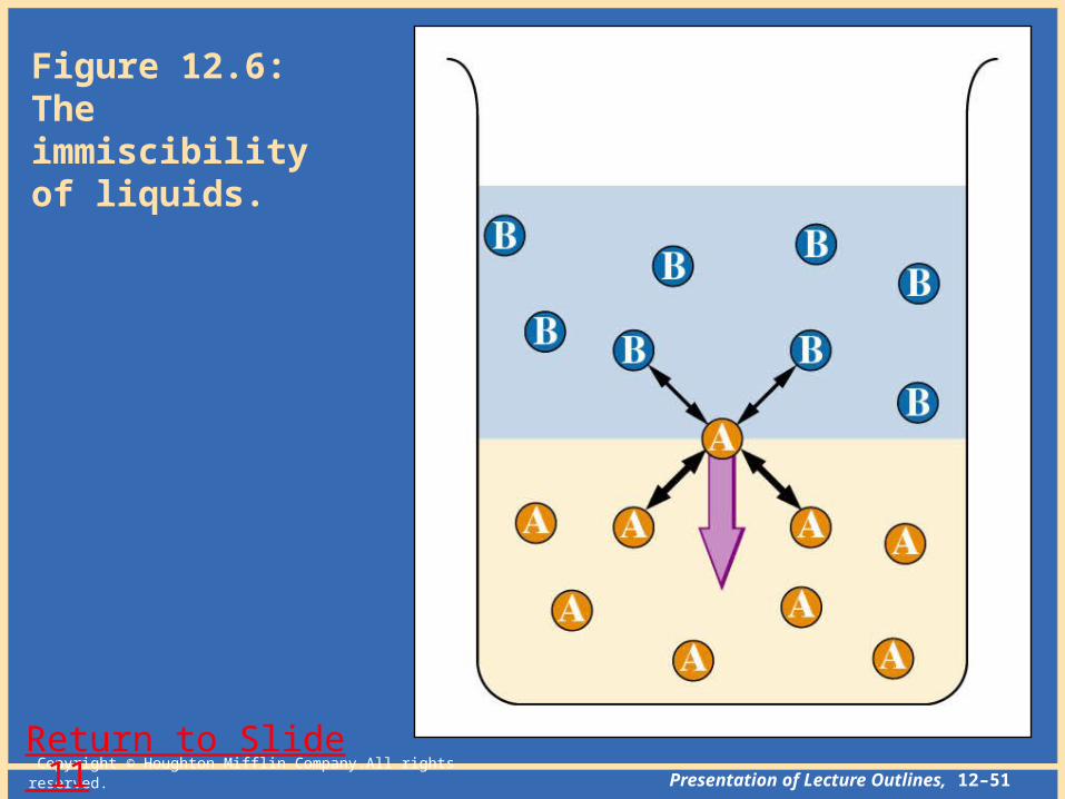
• Nonpolar solutes interact with nonpolar solvents primarily due to London forces.
– Heptane, C7H16, and octane, C8H18, are both nonpolar components of gasoline and are completely miscible liquids.
– However, for water to mix with gasoline, hydrogen bonds must be broken and replaced with weaker London forces between water and the gasoline.
– Therefore gasoline and water are nearly immiscible. (see Figure 12.6 and Table 12.2)

Copyright © Houghton Mifflin Company.All rights reserved. Presentation of Lecture Outlines, 12–12
Ionic Solutions
• Polar solvents, such as water, also interact well with ionic solutes.
– Since ionic compounds are the extreme in polarity, we can illustrate the electrostatic attractions of water for cations and anions. (See Figures 12.8 and 12.9)
+ -H
OH
HO
H
HO
H
HO
H

Copyright © Houghton Mifflin Company.All rights reserved. Presentation of Lecture Outlines, 12–13
Effects of Temperature and Pressure on Solubility
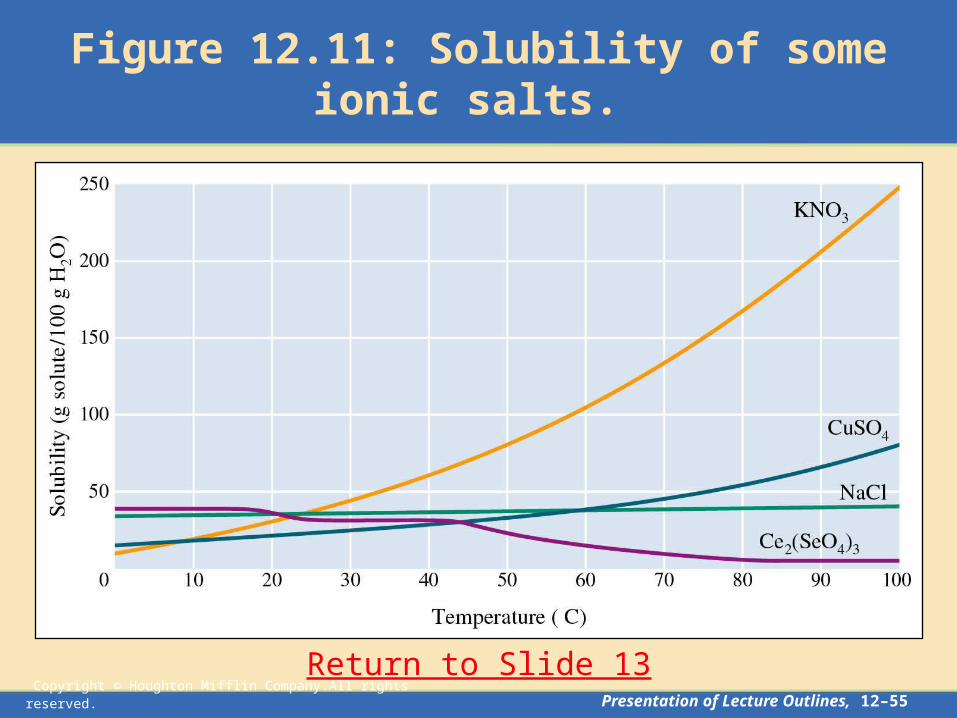
• The solubility of solutes is very temperature dependent.
– For gases dissolved in liquids, as temperature increases, solubility decreases.
– On the other hand, for most solids dissolved in liquids, solubility increases as temperature increases. (See Figure 12.11)

Copyright © Houghton Mifflin Company.All rights reserved. Presentation of Lecture Outlines, 12–14
Temperature Change
• Heat can be evolved or absorbed when an ionic compound dissolves in water.
– This heat of solution can be quite noticeable.– When NaOH dissolves in water, it gets very warm
(the solution process is exothermic).– On the other hand, when ammonium nitrate
dissolves in water, it becomes very cold (the solution process is endothermic). (See Figure 12.12)

Copyright © Houghton Mifflin Company.All rights reserved. Presentation of Lecture Outlines, 12–15
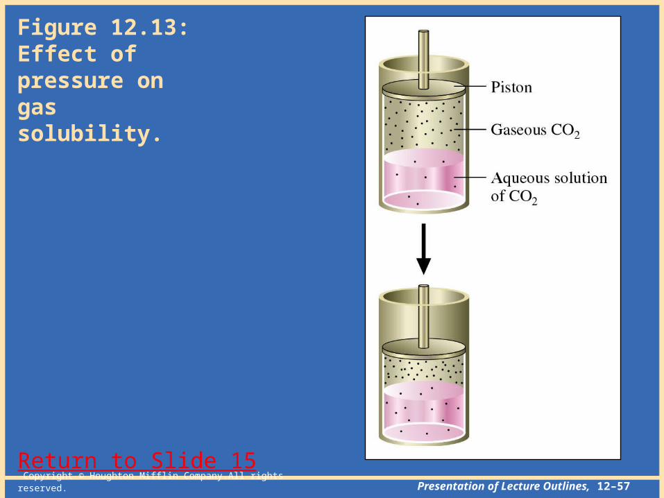
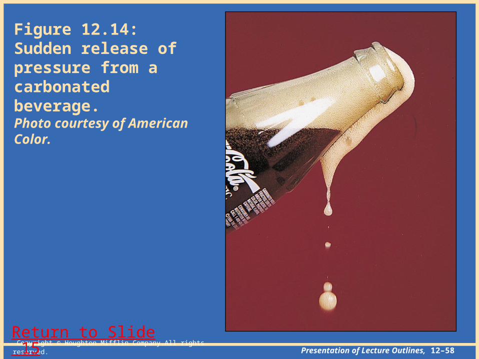
Pressure Change
• Henry’s Law states that the solubility of a gas in a liquid is directly proportional to the partial pressure of the gas in direct contact with the liquid. (See Figures 12.13 ; 12.14;
– Expressed mathematically, the law is
where S is the solubility of the gas, kH is the Henry’s law constant characteristic of the solution, and P is the partial pressure of the gas.
PkS H
Copyright © Houghton Mifflin Company.All rights reserved. Presentation of Lecture Outlines, 12–16
Colligative Properties of Solutions
• The colligative properties of solutions are those properties that depend on solute concentration.
– These properties include:
1. vapor pressure reduction
2. freezing point depression
3. boiling point elevation
4. osmosis– First, we must look into ways of expressing the
concentration of a solution.

Copyright © Houghton Mifflin Company.All rights reserved. Presentation of Lecture Outlines, 12–17
Ways of Expressing Concentration
• Concentration expressions are a ratio of the amount of solute to the amount of solvent or solution.
– The quantity of solute, solvent, or solution can be expressed in volumes or in molar or mass amounts.
– Thus, there are several ways to express the concentration of a solution.

Copyright © Houghton Mifflin Company.All rights reserved. Presentation of Lecture Outlines, 12–18
Molarity
• The molarity of a solution is the moles of solute in a liter of solution.
– For example, 0.20 mol of ethylene glycol dissolved in enough water to give 2.0 L of solution has a molarity of
solution of literssolute of moles
)M(Molarity
glycol ethylene M 10.0solution L 0.2 glycol ethylene mol 20.0

Copyright © Houghton Mifflin Company.All rights reserved. Presentation of Lecture Outlines, 12–19
Mass Percentage of Solute
• The mass percentage of solute is defined as:
– For example, a 3.5% sodium chloride solution contains 3.5 grams NaCl in 100.0 grams of solution.
100% solution of masssolute of mass
solute of percentage Mass
Copyright © Houghton Mifflin Company.All rights reserved. Presentation of Lecture Outlines, 12–20
Molality
• The molality of a solution is the moles of solute per kilogram of solvent.
– For example, 0.20 mol of ethylene glycol dissolved in 2.0 x 10³ g (= 2.0 kg) of water has a molality of
solvent of kilogramssolute of moles
)(molality m
glycol ethylene 10.0solvent kg 0.2 glycol ethylene mol 20.0 m

Copyright © Houghton Mifflin Company.All rights reserved. Presentation of Lecture Outlines, 12–21
A Problem to Consider
• What is the molality of a solution containing 5.67 g of glucose, C6H12O6, dissolved in 25.2 g of water?
– First, convert the mass of glucose to moles.
– Then, divide it by the kilograms of solvent (water).
6126
61266126 OHC g 180.2
OHC mol 1 OHC g 67.5 6126 OHC mol 0.0315
solvent kg 10 25.2
OHC mol 0.0315 Molality 3-
61266126 OHC 1.25m
Copyright © Houghton Mifflin Company.All rights reserved. Presentation of Lecture Outlines, 12–22
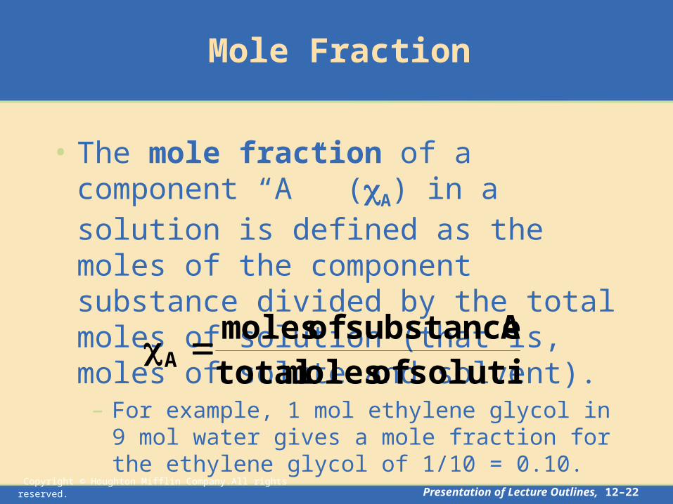
• The mole fraction of a component “A” (A) in a solution is defined as the moles of the component substance divided by the total moles of solution (that is, moles of solute and solvent).
– For example, 1 mol ethylene glycol in 9 mol water gives a mole fraction for the ethylene glycol of 1/10 = 0.10.
solution of moles total Asubstance of moles
A
Mole Fraction
Copyright © Houghton Mifflin Company.All rights reserved. Presentation of Lecture Outlines, 12–23
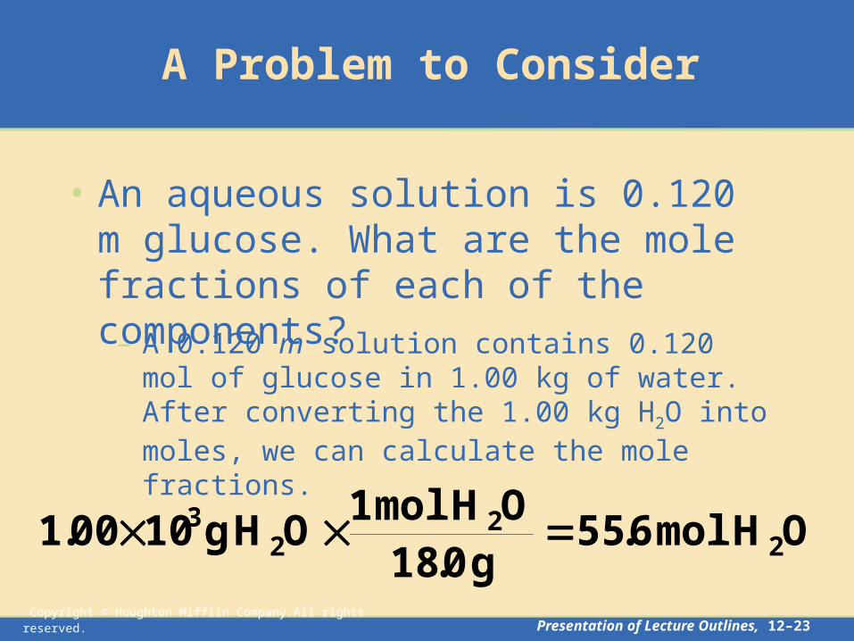
A Problem to Consider
• An aqueous solution is 0.120 m glucose. What are the mole fractions of each of the components?
– A 0.120 m solution contains 0.120 mol of glucose in 1.00 kg of water. After converting the 1.00 kg H2O into moles, we can calculate the mole fractions.
OH mol 6.55g 0.18
OH mol 1OH g10 00.1 2
22
3

Copyright © Houghton Mifflin Company.All rights reserved. Presentation of Lecture Outlines, 12–24
A Problem to Consider
• An aqueous solution is 0.120 m glucose. What are the mole fractions of each of the components?
00215.0mol 55.6) (0.120
mol 120.0ecosglu
998.0mol 55.6) (0.120
mol 6.55water
Copyright © Houghton Mifflin Company.All rights reserved. Presentation of Lecture Outlines, 12–25
– Vapor pressure lowering is a colligative property equal to the vapor pressure of the pure solvent minus the vapor pressure of the solution.
– In 1886, Francois Marie Raoult observed that the vapor pressure of a solution depended on the mole fraction of the solvent.
Vapor Pressure of a Solution
• Chemists have observed that the vapor pressure of a volatile solvent can be reduced by the addition of a nonvolatile solute.

Copyright © Houghton Mifflin Company.All rights reserved. Presentation of Lecture Outlines, 12–26
Vapor Pressure of a Solution
• Raoult’s law states that the vapor pressure of a solution containing a nonelectrolyte nonvolatile solute is proportional to the mole fraction of the solvent. (See Figure 12.16)
where Psolution is the vapor pressure of the solution, solvent is the mole fraction of the solvent, and Po
solvent is the pure vapor pressure of the solvent.
))(P(P solventosolventsolution

Copyright © Houghton Mifflin Company.All rights reserved. Presentation of Lecture Outlines, 12–27
Vapor Pressure of a Solution
• If a solution contains a volatile solute, then each component contributes to the vapor pressure of the solution.
– In other words, the vapor pressure of the solution is the sum of the partial vapor pressures of the solvent and the solute.
– Volatile compounds can be separated using fractional distillation. (See Figure 12.19)
))(P())(P(P soluteosolutesolvent
osolventsolution

Copyright © Houghton Mifflin Company.All rights reserved. Presentation of Lecture Outlines, 12–28
Boiling Point Elevation
• The normal boiling point of a liquid is the temperature at which its vapor pressure equals 1 atm.
– Because vapor pressure is reduced in the presence of a nonvolatile solute, a greater temperature must be reached to achieve boiling. (See Figure 12.20)
– The boiling point elevation, Tb is a colligative property equal to the boiling point of the solution minus the boiling point of the pure solvent.
Copyright © Houghton Mifflin Company.All rights reserved. Presentation of Lecture Outlines, 12–29
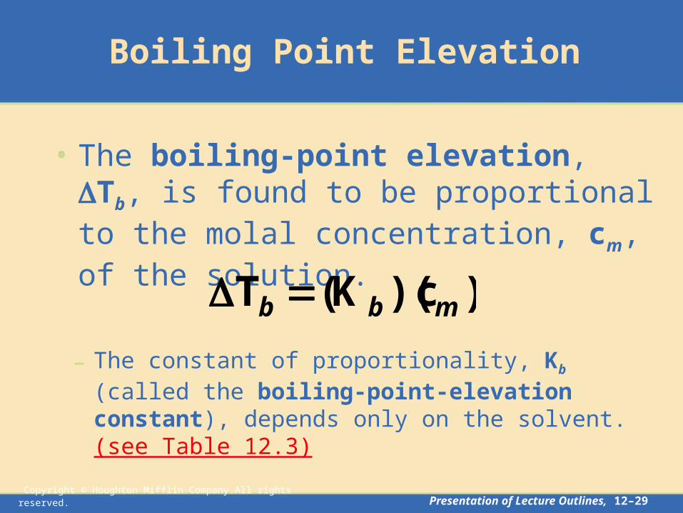
• The boiling-point elevation, Tb, is found to be proportional to the molal concentration, cm, of the solution.
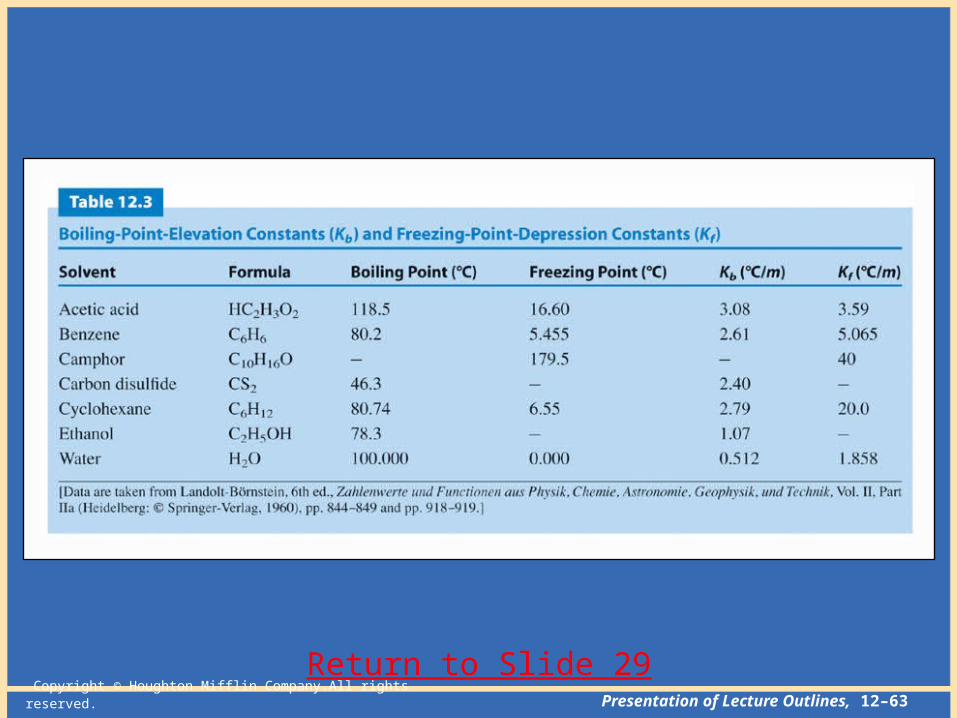
– The constant of proportionality, Kb (called the boiling-point-elevation constant), depends only on the solvent. (see Table 12.3)
)c)(K(T mbb
Boiling Point Elevation

Copyright © Houghton Mifflin Company.All rights reserved. Presentation of Lecture Outlines, 12–30
• The freezing-point depression, Tf, is a colligative property equal to the freezing point of the pure solvent minus the freezing point of a solution.
– Freezing-point depression is also proportional to the molal concentration, cm , of the solute.
)c)(K(T mff – where Kf ,the freezing-point-depression constant,
depends only on the solvent.
Freezing Point Distribution

Copyright © Houghton Mifflin Company.All rights reserved. Presentation of Lecture Outlines, 12–31
– Table 12.3 gives Kb and Kf for water as 0.512 oC/m and 1.86 oC/m, respectively. Therefore,
A Problem to Consider
• An aqueous solution is 0.0222 m in glucose. What are the boiling point and freezing point for this solution?
0.0222 /C0.512 )c)((K T o mmmbb
0.0222 /C1.86 )c)((K T o mmmff C0413.0 o
C0114.0 o
– The boiling point of the solution is 100.011oC and the freezing point is –0.041oC.

Copyright © Houghton Mifflin Company.All rights reserved. Presentation of Lecture Outlines, 12–32
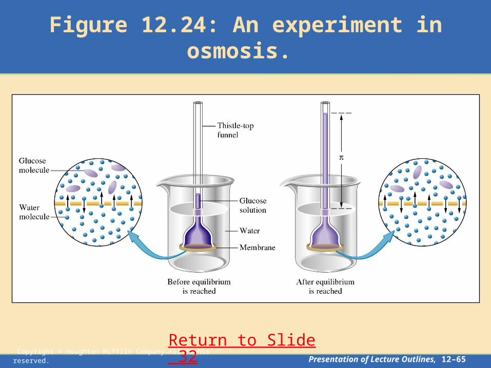
Osmosis
• Certain membranes allow passage of solvent molecules but not solute particles.
– Such a membrane is called semipermeable.– Figure 12.23 depicts the operation of a
semipermeable membrane.– Osmosis is the phenomenon of solvent flow
through a semipermeable membrane to equalize solute concentrations on both sides of the membrane. (See Figure 12.24)
Copyright © Houghton Mifflin Company.All rights reserved. Presentation of Lecture Outlines, 12–33
Osmosis
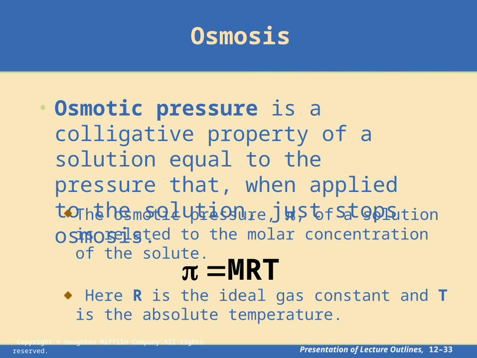
• Osmotic pressure is a colligative property of a solution equal to the pressure that, when applied to the solution, just stops osmosis.
The osmotic pressure, , of a solution is related to the molar concentration of the solute.
MRT Here R is the ideal gas constant and T is the absolute temperature.
Copyright © Houghton Mifflin Company.All rights reserved. Presentation of Lecture Outlines, 12–34
Osmosis
• Osmosis is important in many biological processes.
– A cell might be thought of as an aqueous solution surrounded by a semipermeable membrane (See Figure 12.34).
– The solutions surrounding cells must have the same osmotic pressure. Otherwise, water will either leave the cell, dehydrating it, or enter the cell, causing it to burst.

Copyright © Houghton Mifflin Company.All rights reserved. Presentation of Lecture Outlines, 12–35
Colligative Properties of Ionic Solutions
• The colligative properties of solutions depend on the total concentration of solute particles.
– Consequently, ionic solutes that dissociate in solution provide higher effective solute concentration than nonelectrolytes.
– For example, when NaCl dissolves, each formula unit provides two solute particles.
Copyright © Houghton Mifflin Company.All rights reserved. Presentation of Lecture Outlines, 12–36
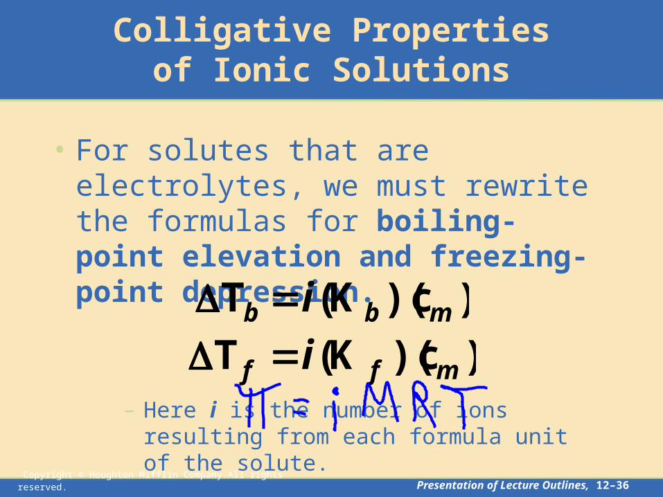
• For solutes that are electrolytes, we must rewrite the formulas for boiling-point elevation and freezing-point depression.
– Here i is the number of ions resulting from each formula unit of the solute.
)c)(K(T mff i)c)(K(T mbb i
Colligative Properties of Ionic Solutions

Copyright © Houghton Mifflin Company.All rights reserved. Presentation of Lecture Outlines, 12–37
A Problem to Consider
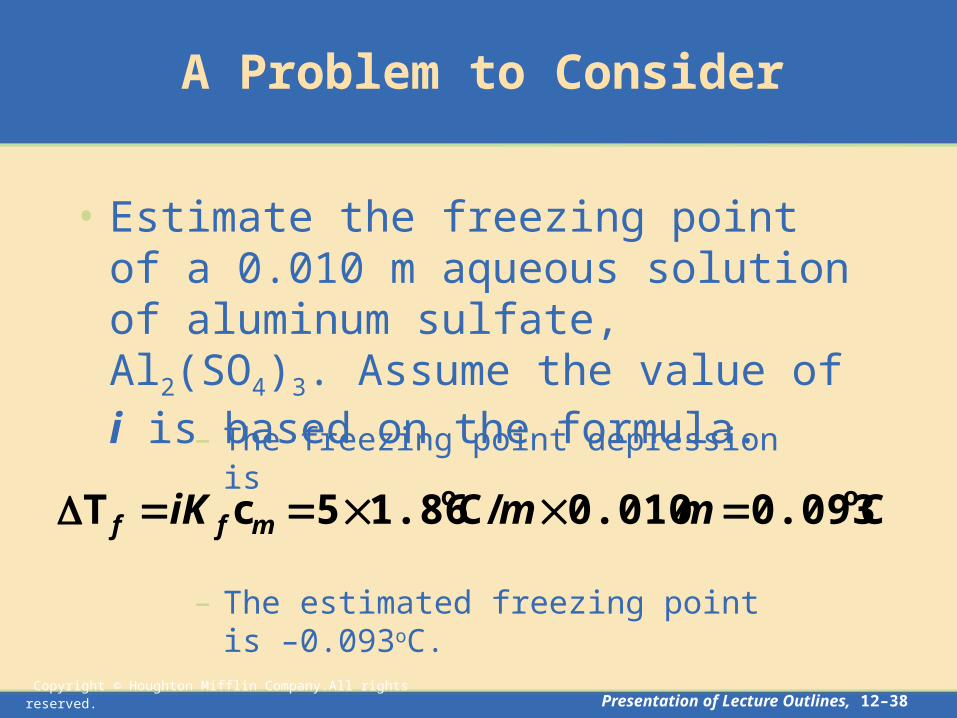
• Estimate the freezing point of a 0.010 m aqueous solution of aluminum sulfate, Al2(SO4)3. Assume the value of i is based on the formula.
(aq)SO 3 (aq) Al2 )s()SO(Al -24
3 OH 342
2
– When aluminum sulfate dissolves in water, it dissociates into five ions.
– Therefore, you assume i = 5.
Copyright © Houghton Mifflin Company.All rights reserved. Presentation of Lecture Outlines, 12–38
A Problem to Consider
• Estimate the freezing point of a 0.010 m aqueous solution of aluminum sulfate, Al2(SO4)3. Assume the value of i is based on the formula.
C0.093 0.010 C/1.86 5 c T oo mmiK mff
– The freezing point depression is
– The estimated freezing point is –0.093oC.
Copyright © Houghton Mifflin Company.All rights reserved. Presentation of Lecture Outlines, 12–39
Colloids
• A colloid is a dispersion of particles of one substance (the dispersed phase) throughout another substance or solution (the continuous phase).
– A colloid differs from a true solution in that the dispersed particles are larger than normal molecules.
– The particles range from 1 x 10³ pm to about 2 x 10⁵ pm.

Copyright © Houghton Mifflin Company.All rights reserved. Presentation of Lecture Outlines, 12–40
The Tyndall Effect
• The scattering of light by colloidal-size particles is known as the Tyndall effect.
– For example, a ray of sunshine passing against a dark background shows up many fine dust particles by light scattering.
– Figure 12.28 illustrates how light is scattered when passing through a colloid but not when passed through a true solution.
Copyright © Houghton Mifflin Company.All rights reserved. Presentation of Lecture Outlines, 12–41
Types of Colloids
• Colloids are characterized according to the state of the dispersed phase and the state of the continuous phase.
– A sol consists of solid particles dispersed throughout a liquid.
– An aerosol consists of liquid droplets or solid particles dispersed throughout a gas.
– An emulsion consists of liquid droplets dispersed throughout another liquid. (see Table 12.4)

Copyright © Houghton Mifflin Company.All rights reserved. Presentation of Lecture Outlines, 12–42
Hydrophilic and Hydrophobic Colloids
• Colloids in which the continuous phase is water are divided into two major classes.
– A hydrophilic colloid is a colloid in which there is a strong attraction between the dispersed phase and the continuous phase (water).
– A hydrophobic colloid is a colloid in which there is a lack of attraction of the dispersed phase for the continuous phase (water).

Copyright © Houghton Mifflin Company.All rights reserved. Presentation of Lecture Outlines, 12–43
Coagulation
• Coagulation is the process by which the dispersed phase of a colloid is made to aggregate and thereby separate from the continuous phase.– Figure 12.29 illustrates how the presence of ions
surrounding colloidal particles can lead to its aggregation.
– Soil suspended in river water coagulates when it meets the concentrated ionic solution of the ocean. The Mississippi Delta was formed this way.

Copyright © Houghton Mifflin Company.All rights reserved. Presentation of Lecture Outlines, 12–44
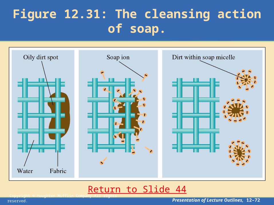
Association Colloids
• A micelle is a colloidal-sized particle formed by the association of molecules, each of which has a hydrophobic end and a hydrophilic end.
– A colloid in which the dispersed phase consists of micelles is called an association colloid.
– Ordinary soap in water provides an example of an association colloid. (See Figures 12.30 and 12.31)
Copyright © Houghton Mifflin Company.All rights reserved. Presentation of Lecture Outlines, 12–45
Operational Skills
• Applying Henry’s law.• Calculating solution concentration.• Converting concentration units.• Calculating vapor-pressure lowering.• Calculating boiling-point elevation and freezing-
point depression.• Calculating molecular weights.• Calculating osmotic pressure.• Determining colligative properties of ionic
solutions.

Copyright © Houghton Mifflin Company.All rights reserved. Presentation of Lecture Outlines, 12–46
Animation: Solution Equilibrium
Return to Slide 2
(Click here to open QuickTime animation)
Copyright © Houghton Mifflin Company.All rights reserved. Presentation of Lecture Outlines, 12–47
Figure 12.1: Immiscible and miscible liquids.Photo courtesy of American Color.
Return to Slide 4

Copyright © Houghton Mifflin Company.All rights reserved. Presentation of Lecture Outlines, 12–48
Animation: Dissolution of a Solid in a Liquid
Return to Slide 5
(Click here to open QuickTime animation)
Copyright © Houghton Mifflin Company.All rights reserved. Presentation of Lecture Outlines, 12–49
Figure 12.3: Comparison of unsaturated and saturated solutions.
Return to Slide 7

Copyright © Houghton Mifflin Company.All rights reserved. Presentation of Lecture Outlines, 12–50
Figure 12.4: Crystallization from a supersaturated solution of sodium acetate.
Return to Slide 8
Copyright © Houghton Mifflin Company.All rights reserved. Presentation of Lecture Outlines, 12–51
Figure 12.6:The immiscibility of liquids.
Return to Slide 11

Copyright © Houghton Mifflin Company.All rights reserved. Presentation of Lecture Outlines, 12–52
Return to Slide 11

Copyright © Houghton Mifflin Company.All rights reserved. Presentation of Lecture Outlines, 12–53
Figure 12.8: Attraction of water molecules to ions because of the ion-dipole force.
Return to Slide 12

Copyright © Houghton Mifflin Company.All rights reserved. Presentation of Lecture Outlines, 12–54
Figure 12.9: The dissolving of lithium fluoride in water.
Return to Slide 12
Copyright © Houghton Mifflin Company.All rights reserved. Presentation of Lecture Outlines, 12–55
Figure 12.11: Solubility of some ionic salts.
Return to Slide 13

Copyright © Houghton Mifflin Company.All rights reserved. Presentation of Lecture Outlines, 12–56
Figure 12.12: Instant cold and hot compress packs.
Photo courtesy of American Color.
Return to Slide 14
Copyright © Houghton Mifflin Company.All rights reserved. Presentation of Lecture Outlines, 12–57
Figure 12.13: Effect of pressure on gas solubility.
Return to Slide 15
Copyright © Houghton Mifflin Company.All rights reserved. Presentation of Lecture Outlines, 12–58
Figure 12.14: Sudden release of pressure from a carbonated beverage.Photo courtesy of American Color.
Return to Slide 15
Copyright © Houghton Mifflin Company.All rights reserved. Presentation of Lecture Outlines, 12–59
Animation: Pressure and Concentration of a Gas
Return to Slide 15
(Click here to open QuickTime animation)

Copyright © Houghton Mifflin Company.All rights reserved. Presentation of Lecture Outlines, 12–60
Figure 12.16: Demonstration of vapor pressure lowering.
Return to Slide 26

Copyright © Houghton Mifflin Company.All rights reserved. Presentation of Lecture Outlines, 12–61
Figure 12.19: Fractional distillation.
Return to Slide 27

Copyright © Houghton Mifflin Company.All rights reserved. Presentation of Lecture Outlines, 12–62
Figure 12.20: Phase diagram showing the effect of nonvolatile solute on freezing point and boiling point.
Return to Slide 28
Copyright © Houghton Mifflin Company.All rights reserved. Presentation of Lecture Outlines, 12–63
Return to Slide 29

Copyright © Houghton Mifflin Company.All rights reserved. Presentation of Lecture Outlines, 12–64
Figure 12.23: A semipermeable membrane separating water and an aqueous solution of glucose.
Return to Slide 32
Copyright © Houghton Mifflin Company.All rights reserved. Presentation of Lecture Outlines, 12–65
Figure 12.24: An experiment in osmosis.
Return to Slide 32

Copyright © Houghton Mifflin Company.All rights reserved. Presentation of Lecture Outlines, 12–66
Animation: Osmosis
Return to Slide 32
(Click here to open QuickTime video)

Copyright © Houghton Mifflin Company.All rights reserved. Presentation of Lecture Outlines, 12–67
Figure 12.34: A model of a cell membrane.
Return to Slide 34

Copyright © Houghton Mifflin Company.All rights reserved. Presentation of Lecture Outlines, 12–68
Figure 12.28: A demonstration of the Tyndall effect by a colloid.
Return to Slide 40

Copyright © Houghton Mifflin Company.All rights reserved. Presentation of Lecture Outlines, 12–69
Return to Slide 41

Copyright © Houghton Mifflin Company.All rights reserved. Presentation of Lecture Outlines, 12–70
Figure 12.29: Layers of ions surrounding charged colloidal particles.
Return to Slide 43

Copyright © Houghton Mifflin Company.All rights reserved. Presentation of Lecture Outlines, 12–71
Figure 12.30: A stearate micelle in water solution.
Return to Slide 44
Copyright © Houghton Mifflin Company.All rights reserved. Presentation of Lecture Outlines, 12–72
Figure 12.31: The cleansing action of soap.
Return to Slide 44