Solution for short-term hydrothermal scheduling with a logarithmic size MILPformulation

Jinbao Jiana,b, Shanshan Pana,∗, Linfeng Yangc

aCollege of Electrical Engineering, Guangxi University, Nanning 530004, ChinabCollege of Science, Guangxi University for Nationalities, Nanning 530006, China

cCollege of Computer Electronics and Information, Guangxi University, Nanning 530004, China

Abstract

Short-term hydrothermal scheduling (STHS) is a non-convex and non-differentiable optimization problem that is difficultto solve efficiently. One of the most popular strategy is to reformulate the complicated STHS by various linearizationtechniques that makes the problem easy to solve. However, in this process, a large number of extra continuous variables,binary variables and constraints will be introduced, which may lead to a heavy computational burden, especially for alarge-scale problem. In this paper, a logarithmic size mixed-integer linear programming (MILP) formulation is proposedfor the STHS, i.e., only a logarithmic number of binary variables and constraints are required to piecewise linearizethe nonlinear functions of STHS. Based on such an MILP formulation, a global optimal solution is therefore can besolved efficiently. To eliminate the linearization errors and cope with the transmission loss, a differentiable non-linearprogramming (NLP) formulation, which is equivalent to the original non-differentiable STHS is derived. By solving thisNLP formulation via the powerful interior point method (IPM), where the previous global optimal solution of MILPformulation is used as the initial point, a high-quality feasible optimal solution to the STHS can thus be determined.Simulation results show that the proposed logarithmic size MILP formulation is more efficient than the generalizedone and when it is incorporated into the solution procedure, our solution methodology is competitive with currentlystate-of-the-art approaches.

Keywords: Short-term hydrothermal scheduling, piecewise linearize, logarithmic size, mixed-integer linearprogramming, non-linear programming

1. Introduction

Short-term hydrothermal scheduling (STHS) is consid-ered as one of the important issues related to optimal eco-nomic operation in power systems. It refers to the attemptto manage the reservoir storage effectively by utilizing the5

available hydro resources as much as possible over a sched-uled time horizon, while satisfying various system opera-tion constraints, such that the total generation cost of ther-mal units is minimum [1]. Normally, STHS is boiled downto solving a mathematical programming problem, during10

which optimization methods are designed for the solution.However, due to the model is notorious for its non-convexand even more, non-differentiable, many difficulties andchallenges will be encountered in the optimization pro-cess. For example, the non-convex hydropower generation15

function and the power transmission loss make the solutioneasily trapped in a poor local optima; when the valve-pointeffects (VPE) of thermal unit which makes the generationcost function non-differentiable is considered, the classicalmathematical programming-based methods, also known as20

∗Corresponding authorEmail address: sspan@mail.gxu.cn (Shanshan Pan )

derivative-based optimization methods, are no longer suit-able.

In the past decades, a wide range of optimization meth-ods have been proposed for handling the STHS problem,such as network flow (NF) [2, 3], dynamic programming25

(DP) [4], Lagrangian relaxation (LR) [5, 6], mixed-integerlinear programming (MILP)[7–14], semi-definite program-ming (SDP) [15, 16] and heuristic based algorithms [17–36]. Because of intractability of the problem, most of theclassical approaches for the STHS problem consider only30

a subset of the real constraints and simplify the functionsinvolved. For example, in [6, 15], the hydraulic subsystemis described as a simple linear model; in [10, 14, 16], thetransmission system is not included; and in [4, 5, 16] thegeneration cost of thermal unit is considered as a quadrat-35

ic function of the output power, where the VPE occuredin actual operation is ignored. However, heuristic basedalgorithms, which are known for their flexibility and ver-satility, can perform excellently for various STHS formu-lations [37], even though they are non-convex and non-40

differentiable. Due to the stochastic nature of the op-timization process, some intrinsic drawbacks of heuristicmethods exist nevertheless. It is well known that they arequite sensitive to various parameter settings [35]. Besides,

Preprint submitted to Elsevier June 11, 2018

unlike deterministic mathematical programming-based op-45

timization techniques, heuristics give unstable results, thatis, the solution generated in each trial may be different [38].

By contrast, classical methods, also known as determin-istic mathematical programming-based optimization tech-niques, can solve to robust solutions due to the solid math-50

ematical foundation and the availability of powerful soft-ware tools. Therefore, the MILP-based approaches haverecently gained increasing popularity for the STHS [7–14]because of the availability of the state-of-the-art MILPsolvers and efficient modeling tools. In order to apply55

MILP-based approaches, some reformulation techniqueswill be adopted to convert the original nonlinear expres-sions of the STHS, which contains one or more variables,into the piecewise linear formulations. In [7–9], piecewiselinear approximation is formulated through a set of one-60

dimensional functions. Such a one-dimensional method isfavorable for practical use because it is simple to model.To get a better piecewise linear approximation, a morecomplex triangulation method is utilized in [10–12], as itcould provide a more refined model. However, the more65

precise the model is, the more computational burden itwill be encountered. To alleviate the computational bur-den, rectangle method is employed in [13, 14], achieving agood trade-off between computational efficiency and accu-racy.70

However, it is widely recognized that, when MILP-basedapproaches are applied, a large number of extra continu-ous variables, binary variables and constraints will be in-troduced in the reformulation, which may lead to a heavycomputational burden, especially for a large-scale prob-75

lem. In this paper, a logarithmic size MILP formulationis proposed for the STHS, i.e., only a logarithmic num-ber of binary variables and constraints are required topiecewise linearize the nonlinear functions of STHS. Thenon-convex and non-differentiable thermal unit generation80

cost is piecewise linearized by the convex combination ap-proach first, yielding an MILP formulation with a logarith-mic number of binary variables and constraints. And then,the hydro generation function of two variables is subdivid-ed into a number of triangles and approximated with a set85

of piecewise linear functions, which is more accurate thanthe rectangle partitions [13, 14]. Compared with the gen-eralized triangulation [10, 11], “Union Jack” triangulationscheme [39] is utilized in this work, getting a logarithmicsize piecewise linear functions for hydro generation func-90

tion. Consequently, when transmission loss is not includ-ed, a logarithmic size MILP formulation for STHS, whichcan be solved to a global optimal solution directly andefficiently, is formulated.

Since MILP-based approach is adopted for the STH-95

S, some piecewise linearization errors will be occured in-evitably. It means that, the scheduling obtained by solvingthe MILP formulation individually is hard to fully satis-fy the system operation constraints. To eliminate the er-rors caused by the linearizations, the original STHS will100

be solved after the optimization in MILP formulation.

Due to the non-differentiable nature of the STHS, clas-sical derivative-based optimization methods are not suit-able any more. Fortunately, with the help of model refor-mulation, a non-linear programming (NLP) formulation105

of the STHS, which can be immediately solved using thepolynomial-time interior point method (IPM), is derived.

Therefore, in the solution procedure, a logarithmic sizeMILP formulation of STHS is solved by a state-of-the-artMILP solver first, yielding a global optimal solution ef-110

ficiently. And then, by solving the NLP formulation ofSTHS via IPM, where the MILP solution is used as theinitial point of IPM, a high-quality feasible optimal solu-tion to the STHS can thus be determined. While trans-mission loss is considered, this approach also works well.115

The validity and effectiveness of the proposed formulation-s and solution methodology are successfully demonstratedfor three test systems.

The remainder of this paper is organized as follows. Sec-tion 2 describes the mathematical formulation of the STH-120

S. Section 3 and Section 4 derive a logarithmic size MILPformulation and an NLP formulation for the STHS, re-spectively. Section 5 introduces the solution methodology.Section 6 presents simulation results and discussions. Sec-tion 7 offers conclusions.125

2. Mathematical formulation of the STHS

Generally, the generation cost of a hydro unit is assumeto be much less than that of a thermal unit [15]; thus, itcan be negligible in the STHS problem. Hence, the STHSproblem is to minimize the total generation cost of thermal130

units by utilizing the available hydro resources as much aspossible over a scheduled time horizon, while satisfyingvarious system operation constraints.

2.1. Objective function

Conventionally, the generation cost of each thermal unit135

can be modeled as a convex quadratic polynomial:

cquadi (PTi,t) = αi + βiP

Ti,t + γi(P

Ti,t)

2, (1)

where PTi,t is the power output of thermal unit i in period t

and αi, βi and γi are positive coefficients for thermal uniti. When VPE is considered, a recurring rectified sinusoidalfunction140

cvpei (PTi,t) = ei| sin(fi(P

Ti,t − PT

i,min))| (2)

is added to the conventional generation cost, whichmakes the generation cost function non-convex and non-differentiable in nature[40]. Above, PT

i,min is the minimumpower output of thermal unit i, and ei and fi are positivecoefficients of the VPE cost for thermal unit i. Conse-145

quently, the thermal unit generation cost considering VPEcan be expressed as

ci(PTi,t) = cquadi (PT

i,t) + cvpei (PTi,t). (3)

2

The objective function of the STHS problem is mini-mization of total generation cost of multiple thermal units,which can be written as150

min

T∑t=1

NT∑i=1

ci(PTi,t), (4)

where NT and T are the total numbers of thermal unitsand periods, respectively.

2.2. Constraints

The minimized STHS problem should be subject to thefollowing constraints.155

2.2.1. Power balance equations

At each time period the total active power generationshould meet the load demand and the transmission loss ofthe power system, expressed as

NT∑i=1

PTi,t +

NH∑j=1

PHj,t = Dt + PL

t , ∀ t, (5)

where PHj,t is the power output of hydro unit j in period160

t, NH is the total number of hydro units, Dt is the loaddemand in period t and PL

t is the transmission loss inperiod t, which can be calculated based on the B-coefficientmethod and expressed as a quadratic function of the poweroutputs [41]:165

PLt =

NT+NH∑i=1

NT+NH∑j=1

P ∗i,tBi,jP∗j,t, ∀ t, (6)

where Bi,j is the (i, j)-th element of the matrix of thetransmission loss coefficients, B; P ∗i,t represents the poweroutput of the ith thermal or hydro unit in period t.

The power output of hydro unit can be calculated us-ing a nonseparable quadric function of reservoir storage170

volume and water discharge, which is given by

PHj,t =ξj,1V

2j,t + ξj,2Q

2j,t + ξj,3Vj,tQj,t

+ ξj,4Vj,t + ξj,5Qj,t + ξj,6, ∀ j, t,(7)

where ξj,1, ξj,2, ξj,3, ξj,4, ξj,5 and ξj,6 are the coefficients ofhydro unit j; Vj,t is the storage volume of reservoir j inperiod t; Qj,t is the discharge of hydro unit j in period t.

2.2.2. Output capacity limitations175

The output of hydro and thermal units should lie in thedetermined intervals, which can be stated as

PTi,min ≤ PT

i,t ≤ PTi,max, ∀ i, t, (8)

PHj,min ≤ PH

j,t ≤ PHj,max, ∀ j, t, (9)

where PTi,max is the maximum power output of thermal

unit i; PHj,min and PH

j,max are the minimum and maximumpower outputs of hydro unit j, respectively.180

2.2.3. Hydraulic network constraints

The reservoir storage volumes and water dischargesshould meet the physical limitations below

Vj,min ≤ Vj,t ≤ Vj,max, ∀ j, t, (10)

Qj,min ≤ Qj,t ≤ Qj,max, ∀ j, t, (11)

where Vj,min and Vj,max are the minimum and maximumstorage volumes of reservoir j, respectively; Qj,min and185

Qj,max are the minimum and maximum discharges of hy-dro unit j in period t, respectively.

For each reservoir, it must meet the water balance equa-tion as follow

Vj,t = Vj,t−1 + Ij,t −Qj,t − Sj,t+

∑r∈Rj

(Qr,t−τr + Sr,t−τr ), (12)

where Vj,t is the storage volume of reservoir j in period t;190

Ij,t is the natural inflow of reservoir j in period t; Sj,t isthe spillage of reservoir j in period t; Rj is the index setof upstream reservoir(s) of reservoir j; τr is the transfertime of water from reservoir r to immediate downstreamreservoir.195

Lastly, the following initial and final reservoir storagevolumes limits should be satisfied,

Vj,0 = Vj,init, ∀ j, (13)

Vj,24 = Vj,end, ∀ j, (14)

where Vj,0 and Vj,24 are the storage volumes of reservoir jin period 0 and 24, respectively; Vj,init and Vj,end are theinitial and final storage volumes of reservoir j, respectively.200

3. A logarithmic size MILP formulation for theSTHS

3.1. A generalized MILP formulation

In this paper, the convex combination formulation [14]is adopted to piecewise linearise the nonlinear functions of205

STHS. Firstly, Li + 1 break points are chosen over a gen-eration interval [PT

i,min, PTi,max], such that PT

i,min = pTi(0) ≤pTi(1) ≤ · · · ≤ p

Ti(Li)

= PTi,max, where Li is calculated by

Li = dL · fi · (PTi,max − PT

i,min)/πe.

Here L is the number of equal segments on each sin(x)where x belongs to [0, π]. So for any given PT

i,t ∈210

[PTi,min, P

Ti,max], it can be expressed uniquely as a convex

combination of at most two consecutive break points byintroducing some continuous variables λi,t(l) ∈ [0, 1], (l =0, 1, ..., Li); the corresponding function value ci(P

Ti,t) can

thus be approximated by the convex combination of the215

function values in these break points. Consequently, thegeneration cost ci(P

Ti,t) can be approximated as

ci(PTi,t) =

Li∑l=0

λi,t(l)ci(pTi(l)), (15)

3

with some additional constraints

PTi,t =

Li∑l=0

λi,t(l)pTi(l), (16)

Li∑l=0

λi,t(l) = 1, λi,t(l) ≥ 0, (17)

Li∑l=1

xi,t(l) = 1, xi,t(l) ∈ {0, 1}, (18)

λi,t(l−1) ≤ xi,t(l−1) + xi,t(l), (l = 1, ..., Li + 1), (19)

where xi,t(0) = xi,t(Li+1) = 0 in (19). Constraint (18)imposes that only one xi,t(l) takes the value 1, and then220

constraints (17) and (19) impose that at most two consec-utive λi,t(l) values are not 0.

Figure 1: Geometric representation of the generalized triangulation

As seen from (7), PHj,t is a function with respect to Vj,t

and Qj,t, which is defined on the rectangle [Vj,min, Vj,max]×[Qj,min, Qj,max]. This two-variables function, which could225

be non-convex, can be approximated linearly using the fol-lowing triangle method [10, 42, 43]. Firstly, Mj + 1 andNj+1 break points are chosen over intervals [Vj,min, Vj,max]and [Qj,min, Qj,max], such that Vj,min = vj(0) ≤ vj(1) ≤· · · ≤ vj(Mj) = Vj,max and Qj,min = qj(0) ≤ qj(1) ≤230

· · · ≤ qj(Nj) = Qj,max. Using these break points as ver-tices, Mi × Ni rectangles can thus be obtained. For eachrectangle, two triangles can be produced after connect-ing the left lower and right upper vertices(see Fig. 1).For any given (Vj,t, Qj,t), it can be expressed as a con-235

vex combination of the vertices of the triangle contain-ing (Vj,t, Qj,t) by introducing some continuous variablesλi,t(m,n) ∈ [0, 1], (m = 0, 1, ...,Mi, n = 0, 1, ..., Ni); thecorresponding function PH

j,t can thus be approximated bythe convex combination of the function values at these240

vertices. Consequently, the hydro generation function PHj,t

can be approximated as

PHj,t =

Mj∑m=0

Nj∑n=0

λj,t(m,n)pHj(m,n) (20)

with some additional constraints

Vj,t =

Mj∑m=0

Nj∑n=0

λj,t(m,n)vj(m), (21)

Qj,t =

Mj∑m=0

Nj∑n=0

λj,t(m,n)qj(n), (22)

Mj∑m=0

Nj∑n=0

λj,t(m,n) = 1, λj,t(m,n) ≥ 0, (23)

Mj∑m=1

Nj∑n=1

(yj,t(m,n) + zj,t(m,n)) = 1,

yj,t(m,n) ∈ {0, 1}, zj,t(m,n) ∈ {0, 1}, (24)245

λj,t(m−1,n−1) ≤ yj,t(m−1,n−1) + yj,t(m,n−1)

+yj,t(m,n) + zj,t(m−1,n−1)

+zj,t(m−1,n),+zj,t(m,n),

(m = 1, ...,Mj + 1, n = 1, ..., Nj + 1) (25)

where pHj(m,n) denotes the hydro generation at (vj(m), qj(n))and

yj,t(0,∗) = yj,t(∗,0) = yj,t(Mj+1,∗) = yj,t(∗,Nj+1) = 0,

zj,t(0,∗) = zj,t(∗,0) = zj,t(Mj+1,∗) = zj,t(∗,Nj+1) = 0.

Above-mentioned yj,t(m,n) and zj,t(m,n) are binary vari-ables that are associated to the upper and lower trianglein the (m,n)-th rectangle. Constraint (24) imposes that,250

among all triangles, only one is adopted for the convexcombination. Then, constraints (23) and (25) impose thatonly the λj,t(m,n) associated with the three vertices in oneof the triangle are not 0.

As a result, a generalized MILP formulation, denoted as255

G-MILP, for the STHS without transmission loss is formu-lated,

min

T∑t=1

NT∑i=1

Li∑l=0

λi,t(l)ci(pTi(l))

s.t. (5), (8)− (14), (16)− (25),

(26)

where PLt = 0 in (5). In this formulation, a number of ex-

tra continuous variables, binary variables and constraintsare introduced, which will cause a heavy computational260

burden, especially for a large-scale problem. In order tosave computational effort, a new piecewise linear modelingtechnique presented in [44], which requires only a logarith-mic number of binary variables and constraints to approx-imate the one and two variables nonlinear functions, is265

employed for the STHS. This is because the computation-al efficiency of an MILP formulation depends much moreon the number of binary variables and constraints than thenumber of continuous variables [45], reducing constraintsand binary variables can make a more significant impact270

than reducing continuous variables on the computation-al efficiency. Next, we will follow the basic idea in [44]to construct a logarithmic size MILP formulation for theSTHS.

4

3.2. A logarithmic size MILP formulation275

In this subsection, the subscripts of thermal units andperiods are dropped to simplify the expressions. Let usintroduce the following additional notations.J = {0, 1, ..., L}, index set of break points.I = {1, ..., L}, index set of intervals.280

I = {1, ..., L− 1}.Si = {i− 1, i}, ∀i ∈ I .I(j) = {i ∈ I : j ∈ Si}.L(|I|) = {1, ..., log2|I|}.4J = {λ ∈ R|J | :

∑j∈J λj = 1, λj ≥ 0}.285

Let B : I → {0, 1}log2|I| be a bijective function such thatfor all i ∈ I the vectors B(i) and B(i+1) differ in at mostone component. Then

∑j∈J+(k,B)

λj ≤ xk,

∑j∈J 0(k,B)

λj ≤ (1− xk),

λ ∈ 4J , xk ∈ {0, 1},∀k ∈ L(|I|),

(27)

where J +(k,B) = {j : ∀i ∈ I(j), k ∈ σ(B(i)), j ∈ J } andJ 0(k,B) = {j : ∀i ∈ I(j), k /∈ σ(B(i)), j ∈ J }, imposes290

that, at most two consecutive λ variables can take a non-zero value.

Above-mentioned σ(B(i)) is the support set of vectorB(i), which is defined by σ(B(i)) ≡ {k : B(i)k 6= 0}.Based on the definition of I(j), we have295

I(0) = {1}, I(j) = {j, j + 1}(j ∈ I), I(L) = {L}.

Then,

J +(k,B) ={j : k ∈ σ(B(j)) ∩ σ(B(j + 1)), j ∈ I}⋃

{j : k ∈ σ(B(I(j))), j ∈ {0, L}},

J 0(k,B) ={j : k /∈ σ(B(j)) ∪ σ(B(j + 1)), j ∈ I}⋃

{j : k /∈ σ(B(I(j))), j ∈ {0, L}}.

i.e.,

J +(k,B) ={j : B(j)k = B(j + 1)k = 1, j ∈ I}⋃

{j : B(1)k = 1, j ∈ {0}}⋃

{j : B(L)k = 1, j ∈ {L}},

J 0(k,B) ={j : B(j)k = B(j + 1)k = 0, j ∈ I}⋃

{j : B(1)k = 0, j ∈ {0}}⋃

{j : B(L)k = 0, j ∈ {L}}.

Next, we will give an example to illustrate how to con-300

struct the formulation (27) and how it works.Example 1Let J = {0, ..., 4}, I = {1, ..., 4} and (λj)

4(j=0) ∈ 4

J .

Firstly, a bijective function B : {1, 2, 3, 4} → {0, 1}2 can

B(1) B(2) B(3) B(4)

0

0 1

1

1 0

Figure 2: The construction of bijective function B

be constructed as shown in Fig. 2. According to Fig.305

2, the bijective function B can be obtained (see Table 1). Based on the definition of J +(k,B) and J 0(k,B), wehave

Table 1: Bijective function B

B(1) B(2) B(3) B(4)0 0 1 10 1 1 0

J +(1, B) = {3, 4}, J 0(1, B) = {0, 1},J +(2, B) = {2}, J 0(2, B) = {0, 4}.

Then, a logarithmic number of binary variables xk(k ∈{1, 2}) and constraints310

λ ∈ 4J , λ3 + λ4 ≤ x1, λ0 + λ1 ≤ (1− x1),

λ2 ≤ x2, λ0 + λ4 ≤ (1− x2),

impose that at most two consecutive λ variables can takea non-zero value. The Fig. 3 illustrates how these con-straints work. �

Figure 3: The procedure for enforcing at most two consecutive λ arenot 0

Note that, in the above discussion, we assume that, |I|is a power of two. If |I| is not a power of two, we only315

need to complete I to an index set of size 2dlog2|I|e and setthe corresponding λ to 0 in the formulation (27).

This technique can be extended to non-separable twovariables function (7) easily. Different from the general-ized linearization in subsection 3.1(see Fig. 1), the “Union320

Jack” triangulation scheme [39] which is depicted in Fig. 4is utilized to partition [Vj,min, Vj,max]× [Qj,min, Qj,max]. Inthis procedure, the rectangle induced by the triangulationis chosen at first, and then one of the two triangles insidethis rectangle is selected.325

Now let us introduce the following additional notations.J1 = {0, 1, ...,M}, index set of break points.

5

J2 = {0, 1, ..., N}, index set of break points.I1 = {1, ...,M}, index set of intervals.I2 = {1, ..., N}, index set of intervals.330

L(|I1|) = {1, ..., log2|I1|}.L(|I2|) = {1, ..., log2|I2|}.4J1×J2 = {λ ∈ R|J1|×|J2| :

∑m∈J1

∑n∈J2

λm,n = 1,

λm,n ≥ 0}.335

In this part, |I1| and |I2| are also assumed to be thepower of two. By applying the above-mentioned techniqueto each component, the first phase results to the followingset of constraints

N∑n=0

∑m∈J+

1 (k,B1)

λm,n ≤ x1k,

N∑n=0

∑m∈J 0

1 (k,B1)

λm,n ≤ (1− x1k),

M∑m=0

∑n∈J+

2 (k,B2)

λm,n ≤ x2k,

M∑m=0

∑n∈J 0

2 (k,B2)

λm,n ≤ (1− x2k),

λ ∈ 4J1×J2 , x1k ∈ {0, 1},∀k ∈ L(|I1|),x2k ∈ {0, 1},∀k ∈ L(|I2|),

(28)

where J +1 (k,B1),J +

2 (k,B2) and J 01 (k,B1),J 0

2 (k,B2) are340

the specializations of J +(k,B) and J 0(k,B).

0

1

2

3

4

0 1 2 3 4

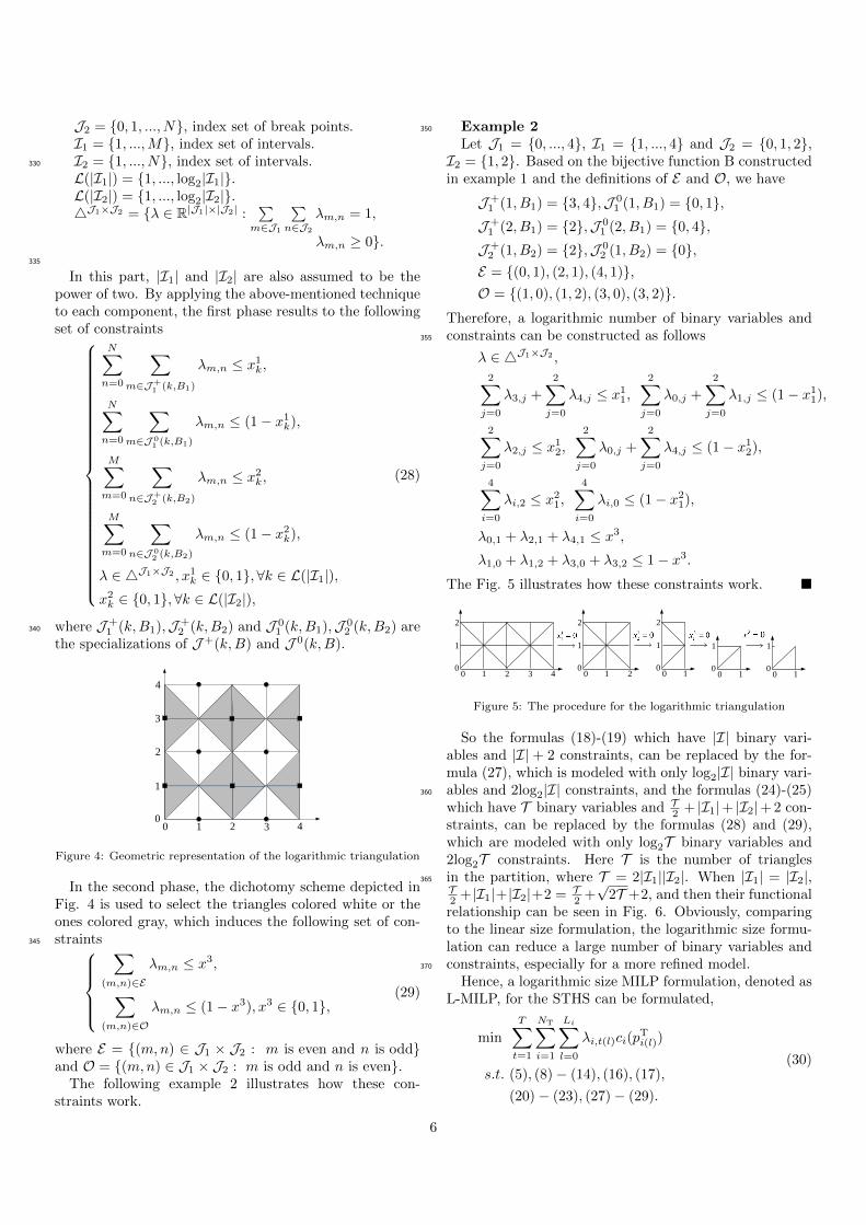
Figure 4: Geometric representation of the logarithmic triangulation

In the second phase, the dichotomy scheme depicted inFig. 4 is used to select the triangles colored white or theones colored gray, which induces the following set of con-straints345

∑(m,n)∈E

λm,n ≤ x3,

∑(m,n)∈O

λm,n ≤ (1− x3), x3 ∈ {0, 1},(29)

where E = {(m,n) ∈ J1 × J2 : m is even and n is odd}and O = {(m,n) ∈ J1 × J2 : m is odd and n is even}.

The following example 2 illustrates how these con-straints work.

Example 2350

Let J1 = {0, ..., 4}, I1 = {1, ..., 4} and J2 = {0, 1, 2},I2 = {1, 2}. Based on the bijective function B constructedin example 1 and the definitions of E and O, we have

J +1 (1, B1) = {3, 4},J 0

1 (1, B1) = {0, 1},J +1 (2, B1) = {2},J 0

1 (2, B1) = {0, 4},J +2 (1, B2) = {2},J 0

2 (1, B2) = {0},E = {(0, 1), (2, 1), (4, 1)},O = {(1, 0), (1, 2), (3, 0), (3, 2)}.

Therefore, a logarithmic number of binary variables andconstraints can be constructed as follows355

λ ∈ 4J1×J2 ,

2∑j=0

λ3,j +

2∑j=0

λ4,j ≤ x11,2∑j=0

λ0,j +

2∑j=0

λ1,j ≤ (1− x11),

2∑j=0

λ2,j ≤ x12,2∑j=0

λ0,j +

2∑j=0

λ4,j ≤ (1− x12),

4∑i=0

λi,2 ≤ x21,4∑i=0

λi,0 ≤ (1− x21),

λ0,1 + λ2,1 + λ4,1 ≤ x3,λ1,0 + λ1,2 + λ3,0 + λ3,2 ≤ 1− x3.

The Fig. 5 illustrates how these constraints work. �

2

1

00 1 2 3 4

2

1

00 1 2

2

1

00 1

1

00 1

1

00 1

Figure 5: The procedure for the logarithmic triangulation

So the formulas (18)-(19) which have |I| binary vari-ables and |I| + 2 constraints, can be replaced by the for-mula (27), which is modeled with only log2|I| binary vari-ables and 2log2|I| constraints, and the formulas (24)-(25)360

which have T binary variables and T2 + |I1|+ |I2|+ 2 con-straints, can be replaced by the formulas (28) and (29),which are modeled with only log2T binary variables and2log2T constraints. Here T is the number of trianglesin the partition, where T = 2|I1||I2|. When |I1| = |I2|,365

T2 +|I1|+|I2|+2 = T

2 +√

2T +2, and then their functionalrelationship can be seen in Fig. 6. Obviously, comparingto the linear size formulation, the logarithmic size formu-lation can reduce a large number of binary variables andconstraints, especially for a more refined model.370

Hence, a logarithmic size MILP formulation, denoted asL-MILP, for the STHS can be formulated,

min

T∑t=1

NT∑i=1

Li∑l=0

λi,t(l)ci(pTi(l))

s.t. (5), (8)− (14), (16), (17),

(20)− (23), (27)− (29).

(30)

6

0 5 10 15 20 25 30 35 40 45 50 55 60 65 70 75 80 85 90 95 1000

20

40

60

80

100

x

y

y = x

y = x +2

y =x

2+√

2x +2

y = log2x

y = 2log2x

Figure 6: The functional relationship of the binary variables andconstraints in two kinds of formulations

4. An NLP formulation for the STHS

Since the non-convex and non-differentiable thermalgeneration cost function and the nonlinear hydro genera-375

tion function of the STHS are both replaced with their lin-ear approximations, some errors will be occured inevitablyin the MILP formulation. So the scheduling obtained bysolving the MILP formulation individually will be hard tofully satisfy the system operation constraints. To eliminate380

these linearization errors, the original STHS will be solvedafter the optimization of the MILP formulation, and thenthe solution feasibility can thus be guaranteed.

However, as seen from section 2, STHS is a non-convexand non-differentiable optimization problem which is in-385

tractable. Due to its non-differentiable nature, classicalmathematical programming-based methods, also knownas derivative-based optimization methods, become invalid.To conquer this difficulty, an auxiliary variable si,t is uti-lized to replace the | sin(fi(P

Ti,t − PT

i,min))| and then, the390

objective function given in (4) can be rewritten to

min

T∑t=1

NT∑i=1

(αi + βiPTi,t + γi(P

Ti,t)

2 + eisi,t) (31)

s.t. si,t ≥ sin(fi(PTi,t − PT

i,min)), (32)

si,t ≥ − sin(fi(PTi,t − PT

i,min)), ∀ i, t. (33)

By introducing some slack variables ui,t and wi,t, theinequality constraints given in (32) and (33) can be con-verted into the following equality constraints [46],

si,t − ui,t − wi,t = 0, (34)

sin(fi(PTi,t − PT

i,min)) + ui,t − wi,t = 0, (35)

ui,t ≥ 0, wi,t ≥ 0, ∀ i, t. (36)

As a result, the original non-convex and non-395

differentiable STHS is equivalent to the following differ-entiable NLP formulation that can be optimized using the

powerful IPM immediately,

min

T∑t=1

NT∑i=1

(αi + βiPTi,t + γi(P

Ti,t)

2 + eisi,t)

s.t. (5)− (14), (34)− (36).

(37)

Remark: Although the NLP formulation for the STHScan be directly solved using the IPM, but it is well known400

that IPM is a local optimization method. If the STHS prob-lem is solved using the IPM in a single step, the optimiza-tion can easily become trapped in a poor local optimum dueto its non-convex nature and multiple local minima.

5. Solution methodology for the STHS405

As it can be seen in previous sections, when transmis-sion loss is not considered, the STHS problem can refor-mulate as a logarithmic size MILP formulation that canbe optimized using a state-of-the-art MILP solver directlyand efficiently. And then, a global optimal solution with-410

in a preset tolerance can be achieved via an enumerationalgorithm. Though the obtaining schedule result satis-fies all the constraints in the MILP formulation, it maylead to power imbalance in the actual operation due tothe linearization errors. To eliminate the errors caused by415

linearization, after the optimization in MILP, the origi-nal STHS, i.e. the NLP formulation given in (37), will besolved again to guarantee the feasibility of the solution.

Consequently, a deterministic solution methodologythat combining MILP-based technique and NLP-based ap-420

proach, denoted as MILP-NLP, is proposed to solve theSTHS problem, which is summarized as follows.

Step 1: Solve the L-MILP formulation (30) by using theMILP-based approach to obtain a global optimal solutionwithin a preset tolerance for the STHS problem.425

Step 2: Solve the NLP formulation (37) by using theIPM, where the initial point is set equal to the solutionobtained in step 1, to obtain a high-quality local feasibleoptimal solution for the STHS problem.

When transmission loss is considered, some transmis-430

sion loss constraints will be involved in the NLP formu-lation (37), which implies that more outputs are requiredto balance the power balance equations. And because ineach period the transmission loss is small compared withthe load demand, the global optimal solution yielding in435

step 1 can be regarded as an approximated solution forthe STHS with transmission loss [46]. Therefore, whenthe NLP formulation is solved in step 2, based on suchan approximated solution obtained in step 1, the output-s of the units will be fine-tuned via IPM, to satisfy the440

new constraints, and then, a high-quality feasible optimalsolution can be expected.

6. Simulation results and discussions

In this section, several test systems that are widely s-tudied for STHS over a scheduled time horizon of 24 h445

7

are adopted to assess the validity and effectiveness of theproposed formulations and solution methodology. First-ly, a system with three thermal units and four cascad-ed hydro reservoirs is carried out, suggesting that solvingthe proposed L-MILP formulation is more efficient than450

the G-MILP formulation and our solution methodologyMILP-NLP is an effective approach for non-convex andnon-differentiable STHS problem. Here, two cases, withand without transmission loss constraints, are considered.And then, two larger systems, one consisting of ten ther-455

mal units and four cascaded hydro reservoirs, another con-sisting of forty thermal units and ten cascaded hydro reser-voirs, are implemented to demonstrate the potential ofMILP-NLP approach for solving large-scale problems. Alltest cases are executed on an Intel Core 2.5 GHz notebook460

with 8 GB of RAM. The models are coded in MATLABR2014a with YALMIP [47] and are optimized using C-PLEX 12.6.1 [48] to solve the L-MILP formulation givenin (30) and IPOPT 3.12.6 [49] to solve the NLP formula-tion given in (37).465

6.1. Test system 1

This test system contains three thermal units and fourcascaded hydro reservoirs, each of which has one hydrounit. The system data can be found in [22].

Case 1: STHS without transmission loss470

In this test case, transmission loss is not taken into ac-count for the STHS. First, we directly solve the L-MILPformulation (30) using CPLEX to 0.01% optimality. Inthis formulation, the segment parameters Li, Mi, and Niare set to 6, 13 and 13, respectively. After optimization,475

a global optimal solution for this formulation is obtainedin 1.30s with a total generation cost of $39754.08. Tak-ing this solution as the initial point in step 2, we solvethe NLP formulation (37) using IPOPT with the defaultoptions, obtaining a high-quality feasible optimal solution480

for the STHS with an optimal value of $40004.90 in 1.61s.Whereas, if the G-MILP formulation (26) is utilized instep 1, more than 500s will be required to find a feasiblesolution, which clearly indicates that using the L-MILPformulation in step 1 can make a significant computation-485

al saving.Table 2 compares the results for the total generation cost

obtained using the MILP-NLP approach with other meth-ods for this case. We can see that the proposed MILP-NLPcan obtain a solution with a smaller total generation cost.490

Since a computationally efficient L-MILP formulation isincorporated into the solution procedure, compared withother reported methods, our MILP-NLP can solve to abetter solution with less CPU time (see in Table 2).

The optimal dispatch results for case 1 of test system 1495

are given in Table 3 to check the feasibility. Not surprising-ly, our solution can always fully satisfy all the constraintsof the original STHS problem. And the circumstances suchas power balance violations reported in [50] does not oc-cur. This is primarily the result of the rigorous theoretical500

foundations of the IPM.

Table 2: Summary results for Case 1 of test system 1

MethodTotal generation cost ($)

CPU Time (s)Minimum Average Maximum

EP [17] 45063.00 - - -PSO [24] 44740.00 - - 232.73MDE [19] 42611.14 - - 125.00CSA [28] 42440.57 - - 109.12

TLBO [29] 42385.88 42407.23 42441.36 -IQPSO [25] 42359.00 - - -QTLBO [30] 42187.49 42193.46 42202.75 21.60MHDE [20] 41856.50 - - 31.00

DNLPSO [27] 41231.00 41783.00 42367.00 125.00MCDE [1] 40945.75 41380.54 41977.04 50.8

RCGA-AFSA [32] 40913.83 41235.73 41362.58 21.00TLPSOS [14] 40298.28 - - 102

MDNLPSO [27] 40179.00 40637.00 41182.00 123.00PSO [36] 40145.00 - - -

MILP-NLP 40004.90 - - 2.91

Case 2: STHS with transmission lossIn this test case, transmission loss is also considered

for the STHS. In step 1, the same L-MILP formulation issolved as in case 1. And then, we solve the NLP formula-505

tion, where transmission loss constraints are also includedin step 2, obtaining a high-quality feasible optimal solutionwith an optimal value of $41199.14 in 1.70s.

The results for the total generation cost obtained us-ing MILP-NLP approach and other methods are shown in510

Table 4. It is obvious that, when transmission loss is con-sidered, the MILP-NLP can also solve to a solution witha smaller total generation cost in shorter time.

The optimal dispatch results for case 2 of test system 1are given in Table 5 for the feasibility verification.515

Table 4: Summary results for Case 2 of test system 1

MethodTotal generation cost ($)

Time (s)Minimum Average Maximum

SPSO [26] 44980.32 46112.85 49166.68 139.7DE [22] 44862.28 - - 24

QEA [18] 44686.31 - - 19RCGA [32] 43465.24 43643.37 43717.27 32MDE [19] 43435.41 - - -ADE [22] 43222.41 - - 24

CABC [31] 43104.56 - - 32SPPSO [26] 42740.23 43622.14 44346.97 32.7RQEA [18] 42715.69 - - 21MHDE [20] 42679.87 - - 40CDE [22] 42452.99 - - 29

AABC [31] 42381.24 - - 16GSO [34] 42316.39 42339.35 42379.18 617.36

QOGSO [34] 42120.02 42130.15 42145.37 625.07RCGA-AFSA [32] 41707.96 41832.36 41894.63 25

ACDE [22] 41593.48 - - 29MCDE [1] 41586.18 42022.67 42365.84 100.05

DRQEA [18] 41435.76 - - 18PSO [36] 41339.00 - - -

ACABC [31] 41281.75 - - 18MILP-NLP 41199.14 3.00

6.2. Test system 2

This test system contains ten thermal units and fourcascaded hydro reservoirs. The system data is taken from[21]. Here transmission loss is not taken into account.

Similar to above two cases, we solve the L-MILP formu-520

lation first, with the parameters set the same as the cases

8

Table 3: Dispatch results for Case 1 of test system 1

tWater discharge (×104 m3 ) Hydro generation (MW) Thermal generation (MW)

Total (MW)Q1,t Q2,t Q3,t Q4,t PH

1,t PH2,t PH

3,t PH4,t PT

1,t PT2,t PT

3,t

1 9.2353 6.0000 21.9196 6.0000 82.4919 50.1640 31.2163 129.0269 102.6735 124.9079 229.5196 750.00002 6.4305 6.0000 24.4706 6.0000 65.0257 51.2960 8.5071 125.7437 175.0000 124.9079 229.5196 780.00003 6.6402 6.0000 22.3062 6.0000 66.9283 52.9340 18.8447 121.6253 175.0000 124.9079 139.7598 700.00004 8.2707 6.0000 18.8180 6.0000 77.7945 54.5000 34.5422 115.8221 102.6735 124.9079 139.7598 650.00005 8.5466 6.0000 17.7364 6.0000 78.7015 55.5040 37.7075 130.7458 102.6735 124.9079 139.7598 670.00006 8.5120 6.0995 16.5540 7.5861 78.0231 56.6681 41.9634 166.2444 102.6735 124.9079 229.5196 800.00007 9.1058 7.2418 15.9724 11.2162 80.9580 63.9063 43.9920 219.1348 102.6735 209.8158 229.5196 950.00008 7.7809 6.0000 15.6689 9.6777 73.5699 55.8277 44.9644 208.7213 102.6735 294.7237 229.5196 1010.00009 9.3780 8.2307 17.0822 15.1439 83.0104 70.4755 41.0611 268.5362 102.6735 294.7237 229.5196 1090.000010 8.6436 7.3635 17.5698 14.9809 79.7466 65.9178 38.9415 268.4773 102.6735 294.7237 229.5196 1080.000011 8.9821 7.9285 16.9958 16.3632 82.5601 70.0284 40.4857 280.0090 102.6735 294.7237 229.5196 1100.000012 7.3677 6.0000 19.4395 15.2782 72.9836 57.9357 31.2685 271.1356 102.6735 294.7237 319.2794 1150.000013 9.2154 8.8359 18.4823 17.0822 85.0492 75.9697 35.9768 286.0875 102.6735 294.7237 229.5196 1110.000014 9.0613 8.8162 18.1225 17.5698 84.8781 75.9509 37.3795 289.7826 102.6735 209.8158 229.5196 1030.000015 8.0205 7.8684 19.1978 16.9958 78.9517 70.8640 32.7585 285.4170 102.6735 209.8158 229.5196 1010.000016 9.6055 10.3009 16.3786 19.4395 88.6589 83.0726 43.6755 302.5842 102.6735 209.8158 229.5196 1060.000017 9.0654 10.0354 15.8631 18.4823 85.5973 80.1509 45.9420 296.3008 102.6735 209.8158 229.5196 1050.000018 7.8675 9.3639 16.1597 18.1225 77.9853 74.8809 46.4245 293.7925 102.6735 294.7237 229.5196 1120.000019 9.6344 11.9061 14.7104 20.0000 88.2409 83.1250 50.8885 305.1798 103.2304 209.8158 229.5196 1070.000020 7.7841 11.0805 14.8022 20.0000 76.6333 77.9434 51.9853 301.4292 102.6735 209.8158 229.5196 1050.000021 5.0000 7.8239 11.2589 17.1117 54.6031 62.2333 55.1875 280.8751 102.6735 124.9079 229.5196 910.000022 5.8190 10.9151 12.1448 20.0000 62.1067 76.7757 57.7506 296.0257 102.6735 124.9079 139.7598 860.000023 5.1939 11.5376 12.5353 20.0000 56.8194 76.8192 58.7757 290.2445 102.6735 124.9079 139.7598 850.000024 9.8395 14.6521 12.9728 20.0000 90.6747 80.3745 58.9976 284.4000 20.8854 124.9079 139.7598 800.0000

Table 5: Dispatch results for Case 2 of test system 1

tWater discharge (×104 m3 ) Hydro generation (MW) Thermal generation (MW)

Total (MW) Loss (MW)Q1,t Q2,t Q3,t Q4,t PH

1,t PH2,t PH

3,t PH4,t PT

1,t PT2,t PT

3,t

1 9.4183 6.0175 21.0278 6.0000 83.3797 50.2788 36.1580 129.0269 102.6735 124.9079 229.5196 755.9443 5.94432 9.6006 6.6809 19.8024 6.0000 84.0892 55.6332 37.7520 125.7437 128.6221 124.9079 229.5196 786.2676 6.26763 6.9200 6.0000 21.9509 6.0000 68.1272 52.5591 23.5725 121.6253 175.0000 124.9079 139.7598 705.5517 5.55174 8.7319 6.0681 18.9982 6.0000 79.2733 54.5983 37.4206 115.8221 102.6735 124.9079 139.7598 654.4555 4.45555 8.5297 6.3078 18.4370 6.3569 77.2744 57.1758 38.8791 134.3918 102.6735 124.9079 139.7598 675.0622 5.06226 8.6072 6.8029 17.8121 8.4475 77.1515 60.7090 41.4080 171.2475 102.6735 124.9079 229.5196 807.6169 7.61697 7.7284 6.0000 17.5245 7.8968 71.9732 55.0676 42.3597 176.1912 175.0000 209.8158 229.5196 959.9271 9.92718 8.1467 6.3306 16.0100 10.5479 74.8542 57.7741 46.7192 215.4912 102.6735 294.7237 229.5196 1021.7554 11.75549 7.9369 6.2355 18.4754 11.7460 74.2279 57.9663 38.3366 234.4268 175.0000 294.7237 229.5196 1104.2009 14.200910 9.1558 8.4206 18.1264 15.8331 81.8924 72.4830 38.4571 275.9498 102.6735 294.7237 229.5196 1095.6990 15.699011 9.4314 8.7621 16.9505 17.5245 84.1736 74.5719 41.5973 289.4452 102.6735 294.7237 229.5196 1116.7047 16.704712 7.5402 6.3334 17.4891 16.0100 73.5314 59.8485 39.9227 277.4437 102.6735 294.7237 319.2794 1167.4229 17.422913 9.7388 9.7543 18.5710 18.4754 86.8855 79.8443 37.4040 296.2541 102.6735 294.7237 229.5196 1127.3047 17.304714 9.7818 10.1283 17.6726 18.1632 87.7427 81.0836 41.1920 294.0446 102.6735 209.8158 229.5196 1046.0717 16.071715 8.4989 8.7095 18.0309 17.4156 81.1566 73.7926 40.3824 288.1524 102.6735 209.8158 229.5196 1025.4929 15.492916 6.9593 7.3385 18.5129 16.9871 71.1105 65.7774 39.7890 285.3499 175.0000 209.8158 229.5196 1076.3622 16.362217 9.9234 11.2351 15.3680 19.2524 89.6721 84.1591 50.1068 300.7183 102.6735 209.8158 229.5196 1066.6652 16.665218 8.8301 10.5232 15.7122 19.1623 83.4531 78.3831 50.0858 298.6435 102.6735 294.7237 229.5196 1137.4823 17.482319 6.1114 8.8523 15.7677 17.6011 64.2692 68.9760 50.7413 288.3419 175.0000 209.8158 229.5196 1086.6637 16.663720 9.3710 12.2598 14.0783 20.0000 85.9415 81.1667 54.9729 302.6758 102.6735 209.8158 229.5196 1066.7658 16.765821 5.0000 8.4339 12.8578 18.8622 54.4194 64.3818 56.8230 292.0769 102.6735 124.9079 229.5196 924.8021 14.802122 7.2797 13.0391 13.2715 20.0000 73.2468 81.0965 58.2711 294.4058 102.6735 124.9079 139.7598 874.3614 14.361423 6.7587 13.5011 13.8152 20.0000 69.6742 78.1603 59.0164 289.7555 102.6735 124.9079 139.7598 863.9476 13.947624 5.0000 8.2655 16.4732 18.8357 55.0200 56.9056 55.6589 277.7155 102.6735 124.9079 139.7598 812.6413 12.6413

in test system 1. After optimization, a global optimal so-lution is obtained in 1.59s with a total generation cost of$157896.54. Taking this solution as the initial point instep 2, we solve the NLP formulation using IPOPT with525

the default options, obtaining a high-quality feasible opti-mal solution with an optimal value of $158127.84 in 5.14s.However, if the G-MILP formulation is solved in step 1,more than 1000s will be consumed for searching a feasiblesolution.530

The total generation cost obtained using the MILP-NLPapproach are compared with those of other methods in Ta-ble 6. We can also see that MILP-NLP can achieve a solu-tion with a much smaller total generation cost in a shorttime. The optimal dispatch results for this test system are535

given in Tables 7 and 8 for the feasibility checking.

Table 6: Summary results of test system 2

MethodTotal generation cost ($)

CPU Time (s)Minimum Average Maximum

SPSO [26] 189350.63 190560.31 191844.28 108.10MDE [26] 177338.60 179676.35 182172.01 86.50DE [21] 170964.15 - - 96.40IDE [23] 170576.50 170589.60 170608.30 727.06GSO [34] 170511.26 170547.56 170586.91 652.35

QOGSO [34] 170293.21 170321.57 170349.34 661.79SPPSO [26] 167710.56 168688.92 170879.30 24.80MCDE [1] 165331.70 166116.4 167060.60 178.5

RCCRO [33] 164138.65 164140.40 164182.35 22.02ORCCRO[33] 163066.03 163068.77 163134.54 15.74IPCSO [35] 162714.00 162813.00 162953.00 22.65PSO [36] 161292.00 - - -

MILP-NLP 158127.84 - - 6.73

9

Table 7: Hydrothermal generation (MW) for test system 2

tHydro generation Thermal generation

TotalPH1,t PH

2,t PH3,t PH

4,t PT1,t PT

2,t PT3,t PT

4,t PT5,t PT

6,t PT7,t PT

8,t PT9,t PT

10,t

1 75.7365 50.1641 0.0005 201.8992 229.5196 199.5996 94.7998 119.7331 174.5997 139.7331 104.2753 84.8665 98.0603 177.0125 1750.00002 89.4156 64.4318 15.1807 188.7722 229.5196 199.5996 94.7998 119.7331 174.5997 139.7331 104.2753 84.8665 98.0603 177.0125 1780.00003 82.7581 57.8707 11.8917 175.1464 229.5196 199.5996 94.7998 119.7331 124.7331 139.7331 104.2753 84.8665 98.0603 177.0125 1700.00004 85.5214 64.3014 21.2213 157.2936 229.5196 199.5996 94.7998 119.7331 124.7331 139.7331 104.2753 84.8665 98.0603 126.3417 1650.00005 64.5149 52.8821 7.3585 172.9114 229.5196 199.5996 94.7998 119.7331 124.7331 139.7331 104.2753 84.8665 98.0603 177.0125 1670.00006 84.4386 72.2115 35.4962 185.6541 229.5196 199.5996 94.7998 119.7331 174.5997 139.7331 104.2753 84.8665 98.0603 177.0125 1800.00007 76.2897 60.0420 29.4497 197.4594 319.2794 274.3995 94.7998 119.7331 174.5997 139.7331 104.2753 84.8665 98.0603 177.0125 1950.00008 75.3090 59.5410 31.7536 206.7706 319.2794 274.3995 94.7998 119.7331 174.5997 139.7331 104.2753 134.7331 98.0603 177.0125 2010.00009 80.6242 67.9145 37.1837 217.7853 319.2794 274.3995 94.7998 119.7331 224.4662 139.7331 104.2753 134.7331 98.0603 177.0125 2090.000010 75.2941 60.7576 34.3158 223.1400 319.2794 274.3995 94.7998 119.7331 224.4662 139.7331 104.2753 134.7331 98.0603 177.0125 2080.000011 79.6874 66.5305 37.7361 229.5538 319.2794 274.3995 94.7998 119.7331 224.4662 139.7331 104.2753 134.7331 98.0603 177.0125 2100.000012 77.1155 63.9041 37.4469 235.1746 319.2794 274.3995 94.7998 119.7331 224.4662 189.5997 104.2753 134.7331 98.0603 177.0125 2150.000013 77.4971 64.9193 39.8851 241.2061 319.2794 274.3995 94.7998 119.7331 224.4662 139.7331 104.2753 134.7331 98.0603 177.0125 2110.000014 79.6493 67.6859 41.7888 254.1167 319.2794 274.3995 94.7998 119.7331 174.5997 139.7331 104.2753 84.8665 98.0603 177.0125 2030.000015 71.3585 60.9329 40.6619 250.2875 319.2794 274.3995 94.7998 119.7331 174.5997 139.7331 104.2753 84.8665 98.0603 177.0125 2010.000016 81.1664 71.6981 45.4635 274.9128 319.2794 274.3995 94.7998 119.7331 174.5997 139.7331 104.2753 84.8665 98.0603 177.0125 2060.000017 75.6856 67.5241 45.2393 274.7917 319.2794 274.3995 94.7998 119.7331 174.5997 139.7331 104.2753 84.8665 98.0603 177.0125 2050.000018 78.2060 70.6592 47.4940 287.0149 319.2794 274.3995 94.7998 119.7331 174.5997 139.7331 104.2753 134.7331 98.0603 177.0125 2120.000019 74.7376 69.7546 48.9206 289.8280 319.2794 274.3995 94.7998 119.7331 174.5997 139.7331 104.2753 84.8665 98.0603 177.0125 2070.000020 65.1629 65.5876 50.1174 282.3729 319.2794 274.3995 94.7998 119.7331 174.5997 139.7331 104.2753 84.8665 98.0603 177.0125 2050.000021 70.2404 71.3936 52.4883 293.6781 229.5196 199.5996 94.7998 119.7331 174.5997 139.7331 104.2753 84.8665 98.0603 177.0125 1910.000022 70.0901 66.3652 54.5167 296.6950 229.5196 199.5996 94.7998 119.7331 124.7331 139.7331 104.2753 84.8665 98.0603 177.0125 1860.000023 57.9166 67.3167 56.1426 296.2910 229.5196 199.5996 94.7998 119.7331 124.7331 139.7331 104.2753 84.8665 98.0603 177.0125 1850.000024 62.5969 70.4382 57.8260 296.0812 229.5196 199.5996 94.7998 119.7331 124.7331 139.7331 45.0000 84.8665 98.0603 177.0125 1800.0000

Table 8: Water discharge (×104 m3 ) for test system 2t Q1,t Q2,t Q3,t Q4,t

1 8.0055 6.0000 26.2599 13.23472 10.7803 8.2300 23.2996 13.17653 9.4171 6.9744 23.0370 13.27874 10.2806 7.8931 21.3050 13.21925 6.6617 6.0000 23.3397 13.00006 10.4427 9.3415 18.2583 13.00007 8.7648 7.3649 19.5241 13.00008 8.5524 7.3150 18.9438 13.00009 9.5521 8.8183 17.6656 13.000110 8.3449 7.4387 18.3056 13.000011 8.9335 8.3312 17.3874 13.000012 8.3840 7.8738 17.6590 13.000013 8.3092 8.0480 17.2836 13.196814 8.5009 8.4704 16.9952 14.150915 7.1169 7.1917 17.5643 13.386016 8.5299 9.1268 16.1470 15.900517 7.6483 8.5305 16.4122 15.718018 8.0212 9.5300 15.7149 17.259519 7.5274 9.7040 15.3794 17.645620 6.2637 9.0107 15.1265 16.743621 6.9132 10.4160 10.0000 18.577322 6.8680 9.4010 10.3195 19.706223 5.3444 9.8652 10.6491 20.670024 5.8374 11.1248 11.1506 22.5442

6.3. Test system 3

To show the potential of MILP-NLP for solving theSTHS problem, a larger test system that contains fortythermal units and ten cascaded hydro reservoirs is sim-540

ulated. The characteristics of the forty thermal units aretaken from [51]. The hydraulic system is constructed basedon [52]. The characteristics of the hydraulic network andload demands are provided in Appendix.

First, we directly solve the L-MILP formulation using545

CPLEX to 0.2% optimality. In this case, the segment pa-rameters Li, Mi, and Ni are set to 6, 8 and 8, respectively.After optimization, a global optimal solution is obtained in25.55s with a total generation cost of $2200819.68. Tak-ing this solution as the initial point in step 2, we solve550

the NLP formulation using IPOPT with the default op-tions, a feasible optimal solution with an optimal valueof $2201437.44 can be calculated in 18.83s. But if the G-MILP formulation is solved in step 1, more than 1000s willbe expended.555

7. Conclusion

In this paper, a deterministic MILP-NLP approachis proposed for the complicated non-convex and non-differentiable STHS problem. To save computational ef-fort, a logarithmic size L-MILP formulation which can be560

solved to a global optimal solution directly and efficient-ly, is constructed first. However, if the STHS is directlysolved by the L-MILP formulation in a single step, somepiecewise linearization errors will be occured inevitably.Therefore, a differentiable NLP formulation which is e-565

quivalent to the original STHS will be solved to search ahigh-quality feasible optimal solution for the STHS. Thesimulation results show that, the proposed L-MILP formu-lation can provide a significant computational advantageand it is very promising for solving numerous variants of570

the STHS problem. When it is incorporated into the solu-tion procedure, MILP-NLP is competitive with currentlystate-of-the-art approaches.

Appendix

1 2

3

4

5 6

7

8

9

10

Figure 7: Hydraulic network of test system 3

10

Table 9: Transfer time to immediate downstream reservoir (h)r 1, 5 2, 6 3, 7, 9 4, 8, 10τr 2 3 4 0

Table 10: Hydro power generation coefficientsj ξj,1 ξj,2 ξj,3 ξj,4 ξj,5 ξj,6

1, 5 -0.0042 -0.42 0.030 0.90 10.0 -502, 6 -0.0040 -0.30 0.015 1.14 9.5 -70

3, 7, 9 -0.0016 -0.30 0.014 0.55 5.5 -404, 8, 10 -0.0030 -0.31 0.027 1.44 14.0 -90

Table 11: Reservoir inflows (×104 m3 )

ReservoirHour1 2 3 4 5 6 7 8 9 10 11 12

1, 5 10 9 8 7 6 7 8 9 10 11 12 102, 6 8 8 9 9 8 7 6 7 8 9 9 8

3, 7, 9 8.1 8.2 4 2 3 4 3 2 1 1 1 24, 8, 10 2.8 2.4 1.6 0 0 0 0 0 0 0 0 0

ReservoirHour13 14 15 16 17 18 19 20 21 22 23 24

1, 5 11 12 11 10 9 8 7 6 7 8 9 102, 6 8 9 9 8 7 6 7 8 9 9 8 8

3, 7, 9 4 3 3 2 2 2 1 1 2 2 1 04, 8, 10 0 0 0 0 0 0 0 0 0 0 0 0

Table 12: Reservoir characteristics (×104 m3 )j Vj,min Vj,max Vj,init Vj,end Qj,min Qj,max Pj,min Pj,max

1, 5 80 150 100 120 5 15 0 5002, 6 60 120 80 70 6 15 0 5003, 7 100 240 170 170 10 30 0 5004, 8 70 160 120 140 13 25 0 5009 100 400 170 190 10 60 0 50010 70 320 120 160 13 50 0 500

Table 13: Load demands (MW)t 1 2 3 4 5 6 7 8

load 7620 8150 8790 9250 9510 9530 9650 9070t 9 10 11 12 13 14 15 16

load 8590 8100 8620 9230 9620 9670 9700 9530t 17 18 19 20 21 22 23 24

load 9710 9600 9320 9100 8820 8480 8100 7730

Acknowledgement575

This work was supported by the Natural Science Foun-dation of China (11771383, 51407037, 51767003); theNatural Science Foundation of Guangxi (2016GXNSF-DA380019, 2014GXNSFFA118001).

References580

[1] Zhang, J.R., Lin, S., Qiu, W.X.. A modified chaotic differ-ential evolution algorithm for short-term optimal hydrothermalscheduling. International Journal of Electrical Power & EnergySystems 2015;65:159–168. doi:10.1016/j.ijepes.2014.09.041.

[2] Li, C.A., Jap, P.J., Streiffert, D.L.. Implementation of net-585

work flow programming to the hydrothermal coordination inan energy management system. IEEE Transactions on PowerSystems 1993;8(3):1045–1053. doi:10.1109/59.260895.

[3] Oliveira, A.R.L., Soares, S., Nepomuceno, L.. Short term hy-droelectric scheduling combining network flow and interior point590

approaches. International Journal of Electrical Power & Ener-gy Systems 2005;27(2):91–99. doi:10.1016/j.ijepes.2004.07.009.

[4] Yang, J.S., Chen, N.M.. Short term hydrothermal coordinationusing multi-pass dynamic programming. IEEE Transactions on595

Power Systems 1989;4(3):1050–1056. doi:10.1109/59.32598.

[5] Redondo, N.J., Conejo, A.J.. Short-term hydro-thermal co-ordination by lagrangian relaxation: solution of the dual prob-lem. IEEE Transactions on Power Systems 1999;14(1):89–95.doi:10.1109/59.744490.600

[6] Borghetti, A., Frangioni, A., Lacalandra, F., Nucci, C.A.. La-grangian heuristics based on disaggregated bundle methods forhydrothermal unit commitment. IEEE Transactions on PowerSystems 2003;18(1):313–323. doi:10.1109/TPWRS.2002.807114.

[7] Conejo, A.J., Arroyo, J.M., Contreras, J., Villamor, F.A..605

Self-scheduling of a hydro producer in a pool-based electricitymarket. IEEE Transactions on Power Systems 2002;17(4):1265–1272. doi:10.1109/TPWRS.2002.804951.

[8] Borghetti, A., D’Ambrosio, C., Lodi, A., Martello, S.. Anmilp approach for short-term hydro scheduling and unit com-610

mitment with head-dependent reservoir. IEEE Transactionson Power Systems 2008;23(3):1115–1124. doi:10.1109/TPWRS.2008.926704.

[9] Tong, B., Zhai, Q.Z., Guan, X.H.. An milp based formulationfor short-term hydro generation scheduling with analysis of the615

linearization effects on solution feasibility. IEEE Transactionson Power Systems 2013;28(4):3588–3599. doi:10.1109/TPWRS.2013.2274286.

[10] Garcia-Gonzalez, J., Castro, G.A.. Short-term hydro schedul-ing with cascaded and head-dependent reservoirs based on620

mixed-integer linear programming. In: 2001 IEEE Porto PowerTech Proceedings. 2001, p. 1–6. doi:10.1109/PTC.2001.964906.

[11] Wu, L., Shahidehpour, M., Li, Z.Y.. Genco’s risk-constrainedhydrothermal scheduling. IEEE Transactions on Power Systems2008;23(4):1847–1858. doi:10.1109/TPWRS.2008.2004748.625

[12] Li, X., Li, T.J., Wei, J.H., Wang, G.Q., Yeh, W.W.G.. Hydrounit commitment via mixed integer linear programming: A casestudy of the three gorges project, china. IEEE Transactionson Power Systems 2014;29(3):1232–1241. doi:10.1109/TPWRS.2013.2288933.630

[13] Guedes, L.S.M., Maia, P.D.M., Lisboa, A.C., Vieira, D.A.G.,Saldanha, R.R.. A unit commitment algorithm and a compactmilp model for short-term hydro-power generation scheduling.IEEE Transactions on Power Systems 2017;32(5):3381–3390.doi:10.1109/TPWRS.2016.2641390.635

[14] Kang, C.X., Guo, M., Wang, J.W.. Short-term hydrother-mal scheduling using a two-stage linear programming withspecial ordered sets method. Water Resources Management2017;31(11):3329–3341. doi:10.1007/s1126.

[15] Fuentes-Loyola, R., Quintana, V.H.. Medium-term hydrother-640

mal coordination by semidefinite programming. IEEE Trans-actions on Power Systems 2003;18(4):1515–1522. doi:10.1109/TPWRS.2003.811006.

[16] Zhu, Y.N., Jian, J.B., Wu, J.K., Yang, L.F.. Global op-timization of non-convex hydro-thermal coordination based on645

semidefinite programming. IEEE Transactions on Power Sys-tems 2013;28(4):3720–3728. doi:10.1109/TPWRS.2013.2259642.

[17] Basu, M.. An interactive fuzzy satisfying method based onevolutionary programming technique for multiobjective short-term hydrothermal scheduling. Electric Power Systems Re-650

search 2004;69(2):277–285. doi:10.1016/j.epsr.2003.10.003.[18] Wang, Y.Q., Zhou, J.Z., Mo, L., Zhang, R., Zhang, Y.C..

Short-term hydrothermal generation scheduling using differen-tial real-coded quantum-inspired evolutionary algorithm. Ener-gy 2012;44(1):657–671. doi:10.1016/j.energy.2012.05.026.655

[19] Lakshminarasimman, L., Subramanian, S.. Short-termscheduling of hydrothermal power system with cascaded reser-voirs by using modified differential evolution. IEE Proceedings-Generation, Transmission and Distribution 2006;153(6):693–700. doi:10.1049/ip-gtd:20050407.660

[20] Lakshminarasimman, L., Subramanian, S.. A modified hybriddifferential evolution for short-term scheduling of hydrothermalpower systems with cascaded reservoirs. Energy Conversion andManagement 2008;49(10):2513–2521. doi:10.1016/j.enconman.2008.05.021.665

[21] Mandal, K.K., Chakraborty, N.. Differential evolutiontechnique-based short-term economic generation scheduling

11

of hydrothermal systems. Electric Power Systems Research2008;78(11):1972–1979. doi:10.1016/j.epsr.2008.04.006.

[22] Lu, Y.L., Zhou, J.Z., Qin, H., Wang, Y., Zhang, Y.C..670

An adaptive chaotic differential evolution for the short-termhydrothermal generation scheduling problem. Energy Conver-sion and Management 2010;51(7):1481–1490. doi:10.1016/j.enconman.2010.02.006.

[23] Basu, M.. Improved differential evolution for short-term675

hydrothermal scheduling. International Journal of ElectricalPower & Energy Systems 2014;58(1):91–100. doi:10.1016/j.ijepes.2013.12.016.

[24] Mandal, K.K., Basu, M., Chakraborty, N.. Particle swarm op-timization technique based short-term hydrothermal scheduling.680

Applied Soft Computing 2008;8(4):1392–1399. doi:10.1016/j.asoc.2007.10.006.

[25] Sun, C.F., Lu, S.F.. Short-term combined economic emis-sion hydrothermal scheduling using improved quantum-behavedparticle swarm optimization. Expert Systems with Applications685

2010;37(6):4232–4241. doi:10.1016/j.eswa.2009.11.079.[26] Zhang, J.R., Wang, J., Yue, C.Y.. Small population-

based particle swarm optimization for short-term hydrother-mal scheduling. IEEE Transactions on Power Systems2012;27(1):142–152. doi:10.1109/TPWRS.2011.2165089.690

[27] Rasoulzadeh-Akhijahani, A., Mohammadi-Ivatloo, B.. Short-term hydrothermal generation scheduling by a modified dynam-ic neighborhood learning based particle swarm optimization.International Journal of Electrical Power & Energy Systems2015;67:350–367. doi:10.1016/j.ijepes.2014.12.011.695

[28] Swain, R.K., Barisal, A.K., Hota, P.K., Chakrabarti, R..Short-term hydrothermal scheduling using clonal selection algo-rithm. International Journal of Electrical Power & Energy Sys-tems 2011;33(3):647–656. doi:10.1016/j.ijepes.2010.11.016.

[29] Roy, P.K.. Teaching learning based optimization for short-term700

hydrothermal scheduling problem considering valve point effectand prohibited discharge constraint. International Journal ofElectrical Power & Energy Systems 2013;53(1):10–19. doi:10.1016/j.ijepes.2013.03.024.

[30] Roy, P.K., Sur, A., Pradhan, D.K.. Optimal short-term hydro-705

thermal scheduling using quasi-oppositional teaching learningbased optimization. Engineering Applications of Artificial Intel-ligence 2013;26(10):2516–2524. doi:10.1016/j.engappai.2013.08.002.

[31] Liao, X., Zhou, J.Z., Yang, S.O., Zhang, R., Zhang, Y.C.. An710

adaptive chaotic artificial bee colony algorithm for short-termhydrothermal generation scheduling. International Journal ofElectrical Power & Energy Systems 2013;53(1):34–42. doi:10.1016/j.ijepes.2013.04.004.

[32] Fang, N., Zhou, J.Z., Zhang, R., Liu, Y., Zhang, Y.C.. A715

hybrid of real coded genetic algorithm and artificial fish swar-m algorithm for short-term optimal hydrothermal scheduling.International Journal of Electrical Power & Energy Systems2014;62(11):617–629. doi:10.1016/j.ijepes.2014.05.017.

[33] Bhattacharjee, K., Bhattacharya, A., Dey, S.H.N.. Opposi-720

tional real coded chemical reaction based optimization to solveshort-term hydrothermal scheduling problems. InternationalJournal of Electrical Power & Energy Systems 2014;63:145–157.doi:10.1016/j.ijepes.2014.05.065.

[34] Basu, M.. Quasi-oppositional group search optimization for725

hydrothermal power system. International Journal of Electri-cal Power & Energy Systems 2016;81:324–335. doi:10.1016/j.ijepes.2016.02.051.

[35] Narang, N.. Short-term hydrothermal generation schedul-ing using improved predator influenced civilized swarm opti-730

mization technique. Applied Soft Computing 2017;58:207–224.doi:10.1016/j.asoc.2017.04.065.

[36] Cavazzini, G., Pavesi, G., Ardizzon, G.. A novel two-swarmbased pso search strategy for optimal short-term hydro-thermalgeneration scheduling. Energy Conversion and Management735

2018;164:460–481. doi:10.1016/j.enconman.2018.03.012.[37] Nazari-Heris, M., Mohammadi-Ivatloo, B., Gharehpetian,

G.B.. Short-term scheduling of hydro-based power plants con-

sidering application of heuristic algorithms: A comprehensivereview. Renewable & Sustainable Energy Reviews 2017;74:116–740

129. doi:10.1016/j.rser.2017.02.043.[38] Xia, X., Elaiw, A.M.. Optimal dynamic economic dispatch

of generation: a review. Electric Power Systems Research2010;80(8):975–986. doi:10.1016/j.epsr.2009.12.012.

[39] Todd, M.J.. Union jack triangulations. Fixed Points 1977;:315–745

336doi:10.1016/B978-0-12-398050-2.50021-9.[40] Walters, D.C., Sheble, G.B.. Genetic algorithm solution of eco-

nomic dispatch with valve point loading. IEEE Transactions onPower Systems 1993;8(3):1325–1332. doi:10.1109/59.260861.

[41] Saadat, H.. Power System Analysis. New York: McGraw-Hill;750

1996.[42] Babayev, D.A.. Piece-wise linear approximation of functions of

two variables. Journal of Heuristics 1997;2(4):313–320. doi:10.1007/BF00132502.

[43] DAmbrosio, C., Lodi, A., Martello, S.. Piecewise linear755

approximation of functions of two variables in MILP models.Operations Research Letters 2010;38(1):39–46. doi:10.1016/j.orl.2009.09.005.

[44] Vielma, J.P., Nemhauser, G.L.. Modeling disjunctive con-straints with a logarithmic number of binary variables and760

constraints. Mathematical Programming 2011;128(1-2):49–72.doi:10.1007/s10107-009-0295-4.

[45] Till, J., Engell, S., Panek, S., Stursberg, O.. Applied hybridsystem optimization: An empirical investigation of complexity.Control Engineering Practice 2004;12(10):1291–1303. doi:10.765

1016/j.conengprac.2004.04.003.[46] Pan, S.S., Jian, J.B., Yang, L.F.. A hybrid milp and ipm for

dynamic economic dispatch with valve point effect. Internation-al Journal of Electrical Power & Energy Systems 2018;97:290–298. doi:10.1016/j.ijepes.2017.11.004.770

[47] Lofberg, J.. Yalmip : A toolbox for modeling and optimizationin matlab. In: In Proceedings of the CACSD Conference. Taipei,Taiwan; 2004,.

[48] IBM ILOG CPLEX Optimization Studio CPLEX User’sManual. http://www.ibm.com/support/knowledgecenter/en/775

SSSA5P_12.6.1/ilog.odms.studio.help/pdf/usrcplex.pdf;2014.

[49] Wachter, A., Biegler, L.T.. On the implementation of aninterior-point filter line-search algorithm for large-scale nonlin-ear programming. Mathematical Programming 2006;106(1):25–780

57. doi:10.1007/s10107-004-0559-y.[50] Esmaeily, A., Raeisi, F., Ahmadi, A., Ahmadi, M.R.. A

note on short-term hydro-thermal scheduling. Energy Con-version and Management 2016;126:1178–1186. doi:10.1016/j.enconman.2016.08.083.785

[51] Sinha, N., Chakrabarti, R., Chattopadhyay, R.K.. Evolu-tionary programming techniques for economic load dispatch.IEEE Transactions on Evolutionary Computation 2003;7(1):83–94. doi:10.1109/TEVC.2002.806788.

[52] Orero, S.O., Irving, M.R.. A genetic algorithm modelling790

framework and solution technique for short term optimal hy-drothermal scheduling. IEEE Transactions on Power Systems1998;13(2):501–516. doi:10.1109/59.667375.

12