solar powered urban pollution mapping...air pollution is a grave health problem. in 2005, the world...
TRANSCRIPT

Solar Powered Urban Pollution Mapping
A Major Qualifying Project
Submitted to the Faculty of
WORCESTER POLYTECHNIC INSTITUTE
In partial fulfillment of the requirements for the
Degree of Bachelor of Science in
Electrical and Computer Engineering
By
Mateo Carvajal
Report Submitted to:
Professor Susan M. Jarvis
Worcester Polytechnic Institute
April 24, 2017
Project Number:
MQP-SMJ-ABGW
Worcester
This report represents work of WPI undergraduate students submitted to the faculty as evidence of a
degree requirement. WPI routinely publishes these reports on its web site without editorial or peer
review. For more information about the projects program at WPI, see
http://www.wpi.edu/Academics/Projects.

ii
Abstract
Eighty percent of all urban areas in the world report air pollution levels higher
than the standards deemed safe by the World Health Organization. This project explores
the creation of a prototype that can granularly measure air quality in urban areas. The
prototype measures carbon monoxide, nitrogen dioxide, sulfur dioxide, hydrogen sulfide,
ozone and particulate matter. The prototype also acquires the geographical position of the
measurement and reports the data wirelessly to a database. This approach can enable
governments and citizens to foster improvements to urban environments that have high
levels of pollution.

iii
Acknowledgments
I would like to thank Prof. Susan Jarvis for her guidance throughout the project;
her contributions have enhanced this project in many ways. Kayleah Griffen for creating
the power component for the project, a major and key part of the project. Her willingness
to integrate it to the system has resulted in a very rewarding outcome. I would also like to
thank those behind the scenes, who helped move the project forward, Ching-Hsiang Chen
and other close friends who provided the much needed inspiration and support in this
endeavor.
iv
Table of Contents
Abstract ........................................................................................................................................... ii
Acknowledgments.......................................................................................................................... iii
Table of Contents ........................................................................................................................... iv
Table of Figures .............................................................................................................................. v
1. Introduction ............................................................................................................................. 1
2. Background .............................................................................................................................. 3
3. Design ...................................................................................................................................... 6
Sensors ............................................................................................................................. 6
Wireless Data Transmission and GPS ............................................................................ 13
Microcontroller............................................................................................................... 13
Solar Power and Battery ................................................................................................. 14
4. Implementation ...................................................................................................................... 15
Electrochemical Sensors ................................................................................................ 15
Particulate Matter Sensor ............................................................................................... 20
FONA 808 ...................................................................................................................... 24
Atmega 2560 .................................................................................................................. 27
Solar Power and Battery ................................................................................................. 29
Final Hardware Layout................................................................................................... 29
5. Results ................................................................................................................................... 33
6. Conclusion and Recommendations ....................................................................................... 38
7. Bibliography .......................................................................................................................... 39
8. Appendix ............................................................................................................................... 42
Appendix A: Solar Power and Battery ...................................................................................... 42
Appendix B: Bill of Materials (BOM) ...................................................................................... 59
Appendix C: ULPSM Schematic [9] ......................................................................................... 60
Appendix D: Code Listing ........................................................................................................ 61
Main.cpp ................................................................................................................................ 61
Mqpdef.h................................................................................................................................ 62
SpecSensorCode.cpp ............................................................................................................. 65
pmSensorCode.cpp ................................................................................................................ 68
Power.cpp .............................................................................................................................. 71
Ubidots.cpp ............................................................................................................................ 75
Appendix E: MATLAB Practical Model Parameter Extraction Code ...................................... 77
Appendix F: MATLAB Practical Model Characteristic Curve Plotting Code ......................... 78
Appendix G: MATLAB Simulink Practical Model Solar Panel with DC to DC Converter .... 81
Appendix H: Maximum Power Point Tracking Code written in MATLAB ............................. 82
Appendix I: Additional Research .............................................................................................. 84

v
Table of Figures
Figure 1 - Luftmeßnetz Hamburg [8] .............................................................................................. 4
Figure 2 - Concept of operation for distributed pollution monitoring system ................................ 5
Figure 3 – High level Design of the System ................................................................................... 6
Figure 4 - Spec sensor general design [9] ....................................................................................... 7
Figure 5 - SPEC Sensor .................................................................................................................. 7
Figure 6 - SPEC Ultra Low Power Sensor Module (ULPSM) ....................................................... 8
Figure 7 - Shinyei Technology Particulate Matter Sensor [15] .................................................... 12
Figure 8 – Overall System Signal Diagram .................................................................................. 15
Figure 9 - SPEC ULPSM Layout.................................................................................................. 16
Figure 10 - Spec Sensor Connection to Buffer Amplifier ............................................................ 17
Figure 11 - ULPSM Vgas and Vref Output .................................................................................. 19
Figure 12 - NTC Murata NCP18WM474J03RB Thermistor Layout ........................................... 19
Figure 13 - Shinyei Particulate Matter Sensor Layout.................................................................. 20
Figure 14 - Extracting Two Bytes from Buffer ............................................................................ 21
Figure 15 - Pulse Occupancy Ratio vs Weight Concentration [17] .............................................. 24
Figure 16 - FONA 808 3G and GPS Module Layout ................................................................... 25
Figure 17 - UbidotsFONA Modifications for GPS Acquisition ................................................... 27
Figure 18 - Oscillator Connection to Atmega2560 ....................................................................... 28
Figure 19 - Voltage Regulators in PCB Design ............................................................................ 30
Figure 20 - Overall Schematic without Solar Power and Battery Design .................................... 31
Figure 21 - Top of PCB ................................................................................................................ 32
Figure 22 – Bottom of PCB .......................................................................................................... 32
Figure 23 - Temperature Sensor Results ....................................................................................... 33
Figure 24 - Results from PM Sensor Message.............................................................................. 35
Figure 25 - GPS Response ............................................................................................................ 35
Figure 26 - HTTP Post Command and FONA Response ............................................................. 36
Figure 27 – Sulfur Dioxide Ubidots Results ................................................................................. 36
Figure 28 – Final Prototype of our solar powered pollution measurement system ...................... 37
Figure 29 - Voltage vs Power Curve for 2W Solar Panel ............................................................. 45
Figure 30 - Basic Layout of DC/DC Boost Converter .................................................................. 46
Figure 31 - Inductor Analysis ....................................................................................................... 48
Figure 32 - Solar Charging Boost Converter Topology................................................................ 48
Figure 33 - Voltage Follower and Voltage Divider Circuit .......................................................... 50
Figure 34 - Full Solar Charging System Schematic...................................................................... 51
Figure 35 - Solar Panel Practical Model ....................................................................................... 53
Figure 36 - Characteristic IV and PV Curves for Solar Panel ...................................................... 54
Figure 37 –Duty Cycle Simulations .............................................................................................. 55
Figure 38 - Complete Prototype .................................................................................................... 56
Figure 39 - The IV and PV Characteristic Curves for the Solar Panel ......................................... 57
Figure 40 - Maximum Power Point Tracking Test Case .............................................................. 57

vi
Figure 41 - Voltage Varying as a Result of Irradiance Level Changing ...................................... 58
Figure 42 – Wireless Technologies Comparison .......................................................................... 85

1
1. Introduction
Air pollution is a grave health problem. In 2005, The World Health Organization
(WHO) estimated that 2 Million lives were being lost prematurely due to air pollution
[1]. In 2016, The Global Burden of Disease, a global research program, estimated that the
deaths due to outdoor and household pollution were 5.5 Million [2]. Both studies are
alarming. The future looks even more distressing. The Organization for Economic Co-
operation and Development (OECD), in a 2012 report, estimated that by the year 2050,
the leading cause of premature deaths would be air pollution, ahead of unsafe water and
sanitation [3].
Urban areas are at the frontline of this battle. The WHO reported that 80% of all
urban areas record measurements of pollution that are higher than those recommended for
human health [1]. In urban areas in Asia, the figure rises to 98%.
The main urban air pollutants, also known as primary pollutants as they are
produced directly from the source are Nitrogen Oxides (NOX), Sulfur Oxide, Carbon
Monoxide, Lead and Particulate Matter (PM). Secondary pollutants are those that result
from chemical reactions in the air between the primary pollutants and naturally occurring
gases for example Ozone (O3), Sulfuric Acid (H2SO2) and Nitric Acid (HNO3). Excess of
these pollutants can be directly attributed to human activity.
Carbon monoxide is primarily a result of human activity. Mobile sources account
for the biggest fraction of carbon monoxide emissions in the US. Mobile sources are
regarded as those that can move, for example, vehicles (cars & trucks) airplanes,
locomotives and ships. Mobile sources, especially cars and trucks, account for up to 95%
of the carbon monoxide emissions in urban areas [4]. CO is an odorless and colorless gas.
It is a result of fossil fuel combustion. When inhaled, CO is carried in the red blood cells
that normally carry oxygen. This results in less oxygen reaching the brain and other
organs. Resulting in chest pain and headaches at low concentrations. At very high
concentrations, carbon monoxide is lethal. In the US, the Occupational Safety and Health
Administration limits the exposure to 50 ppm.
Nitrogen oxides are the result of combustion processes of nitrogen bearing coals
and oil. When the fuels combust the nitrogen particles are released. These particles form
N2 or NOx. The latter having negative effects on the environment and other living beings.
Exposure to NO2 causes inflammation of the nose and throat. Long-term exposure
increases the risk of respiratory conditions such as asthma, bronchitis or pneumonia and
increases the allergic response to allergens [5]. Concentrations of 10-20 ppm causes
irritation to the throat. 25-50 ppm can cause pulmonary edema, an increase accumulation
of fluids in the lungs. 100 ppm or higher can cause death from asphyxia from liquids in
the lungs.
Hydrogen sulfide is a toxic and flammable gas. At low concentrations (10-50
ppm), H2S irritates soft tissue like eyes and throat. Long exposure can cause eye
inflammation, headache insomnia and fatigue. In addition, moderate concentrations (50-
320 ppm) can cause coughing, difficulty to breathe (pulmonary edema), nausea and
vomiting [6]. High concentrations (>400 ppm can cause, shock, convulsions, rapid

2
unconsciousness within a few breaths, or even a single breath. The largest industrial
source of hydrogen sulfide are petroleum refineries, which liberate sulfur from petroleum
by mixing it with hydrogen. This results in H2S. Hydrogen Sulfide is also released from
biological decay.
Sulphur dioxide anthropogenic emissions are mainly the result of the burning of
fossil fuels such as coal, oil and natural gas. Coal accounts for 50 percent of annual
emissions, oil 25 percent. Volcano eruptions can also release high levels of sulfur
dioxide. High concentrations of SO2 can cause inflammation of soft tissue such as the
eyes, nose, throat and lungs.
Ozone is an important compound in the ozone layer, where it absorbs ultraviolet
radiation and protects the earth. On the ground level, ozone is harmful to health. It is
mainly a result of reactions of pollutants emitted from the burning of fossil fuels.
Particulate matter is a mix of solid and liquid droplets that are found in the air.
Some of the particles are large enough for the human eye to see concentrations of them.
Others are small enough that they can only be seen using an electron microscope.
Different cities suffer from different pollutants. Policies, population density, per
capita emissions, wind direction and topographic barriers all take part in determining the
pollutants that affect a given urban area. In Delhi, India the annual mean concentration of
PM10 (particles 10-µg m-3 or less) is 240-µg m-3, 12 times more than the 20-µg m-3 level
set by the WHO as safe. In the UK nitrogen oxides (NOX) are above the permitted limits
in 40% of Britain’s local authorities. This is in part due to past legislations that
incentivized the use of diesel powered vehicles over gasoline ones. However, British
PM10 is within the permitted values. In New York, the high population density allows for
a greater use of public transportation. In addition, no significant topographic barriers are
present, allowing the wind to blow the pollutants away from their source.
Despite being at a moment in time where scientists know how air pollution is
produced, how it affect us and have taken action to set goals for emissions, the rate at
which people die prematurely has not yet shown signs of decline. More has to happen in
order to revert this lethal trend.
This project aims to provide an affordable, portable and self-reliant tool to
monitor pollution. Providing data to create awareness and inspire targeted corrective
actions by local governments and citizens.

3
2. Background
Air pollution is dispersed uniquely in different environments. Each city, for
example, has different building sizes, wind speed, direction, topographies, traffic flows,
and geographical location. Scientists have struggled to measure pollution effectively
across cities. This is mainly due to the cost of implementing a citywide monitoring
infrastructure. For this reason, mathematical models have been developed to understand
the dispersion of pollution around streets and buildings with limited data sources.
Table 1 – Air Quality Monitoring Stations in Cities around the Globe
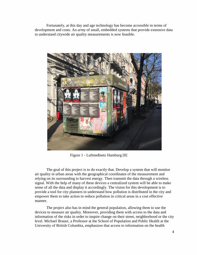
Currently, air quality is measured at city levels. In developed countries, for
example, monitoring stations are found throughout urban areas. The data is then used to
support and enforce environmental policies. The stations are large in order to house high
precision measurement equipment; in Figure 1 one can observe one of these stations in
Hamburg, Germany. The pictured station is located on Stresemannstraße. It has been
recording data since October 24, 1991. It currently records data on Air pollutants such as
particulate matter (PM10) nitrogen oxide, nitrogen dioxide and nitrogen oxides at
different heights, mainly 1.5, 3.5, 4.0 meters above ground [7]. Since this station started
monitoring It has changed the gases it can sense, mainly due to the shifting challenges
that cities face with improvements in new technologies.
Different cities have different capabilities to monitor and control air quality. New
York uses 150 monitoring stations to control air quality. London has at least a monitoring
station for each of each of its 33 boroughs. Delhi has 28 monitoring stations. Bogota,
Colombia uses 14 stations. Mexico City, 30. Hamburg, 16. What is particularly
interesting is how many stations one can find in some cities and how few you can find in
others as seen on the Table 1. Some cities are lacking the infrastructure to monitor and
control air pollutants.
All the data that is being collected can be used to save lives. Nonetheless, more
data could be collected in order to create an extensive database that can be used in
helping plan urban spaces effectively to reduce the negative effects of air pollution on
citizens.
City, Country Population
(Million)
Area
(km2)
Number of
Monitoring Stations
New York City, USA 8.5 789 150
London, UK 8.7 1,738 33
Bogota, Colombia 8.0 1,775 14
Mexico City, Mexico 8.8 1,485 30
Delhi, India 19.0 1,484 30
Hamburg, Germany 1.8 755 16
4
Fortunately, at this day and age technology has become accessible in terms of
development and costs. An army of small, embedded systems that provide extensive data
to understand citywide air quality measurements is now feasible.
Figure 1 - Luftmeßnetz Hamburg [8]
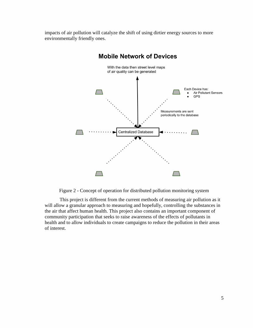
The goal of this project is to do exactly that. Develop a system that will monitor
air quality in urban areas with the geographical coordinates of the measurement and
relying on its surrounding to harvest energy. Then transmit the data through a wireless
signal. With the help of many of these devices a centralized system will be able to make
sense of all the data and display it accordingly. The vision for this development is to
provide a tool for city planners to understand how pollution is distributed in the city and
empower them to take action to reduce pollution in critical areas in a cost effective
manner.
The project also has in mind the general population, allowing them to use the
devices to measure air quality. Moreover, providing them with access to the data and
information of the risks in order to inspire change on their street, neighborhood or the city
level. Michael Brauer, a Professor at the School of Population and Public Health at the
University of British Columbia, emphasizes that access to information on the health
5
impacts of air pollution will catalyze the shift of using dirtier energy sources to more
environmentally friendly ones.
Figure 2 - Concept of operation for distributed pollution monitoring system
This project is different from the current methods of measuring air pollution as it
will allow a granular approach to measuring and hopefully, controlling the substances in
the air that affect human health. This project also contains an important component of
community participation that seeks to raise awareness of the effects of pollutants in
health and to allow individuals to create campaigns to reduce the pollution in their areas
of interest.
6
3. Design
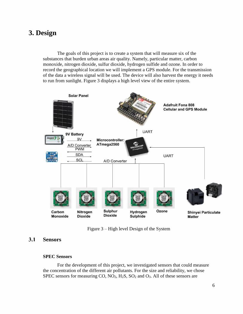
The goals of this project is to create a system that will measure six of the
substances that burden urban areas air quality. Namely, particular matter, carbon
monoxide, nitrogen dioxide, sulfur dioxide, hydrogen sulfide and ozone. In order to
record the geographical location we will implement a GPS module. For the transmission
of the data a wireless signal will be used. The device will also harvest the energy it needs
to run from sunlight. Figure 3 displays a high level view of the entire system.
Figure 3 – High level Design of the System
Sensors
SPEC Sensors
For the development of this project, we investigated sensors that could measure
the concentration of the different air pollutants. For the size and reliability, we chose
SPEC sensors for measuring CO, NO2, H2S, SO2 and O3. All of these sensors are
7
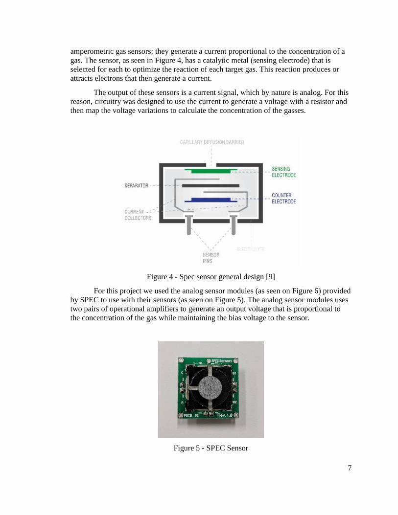
amperometric gas sensors; they generate a current proportional to the concentration of a
gas. The sensor, as seen in Figure 4, has a catalytic metal (sensing electrode) that is
selected for each to optimize the reaction of each target gas. This reaction produces or
attracts electrons that then generate a current.
The output of these sensors is a current signal, which by nature is analog. For this
reason, circuitry was designed to use the current to generate a voltage with a resistor and
then map the voltage variations to calculate the concentration of the gasses.
Figure 4 - Spec sensor general design [9]
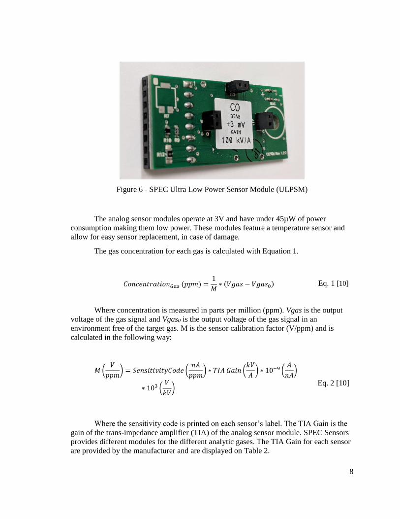
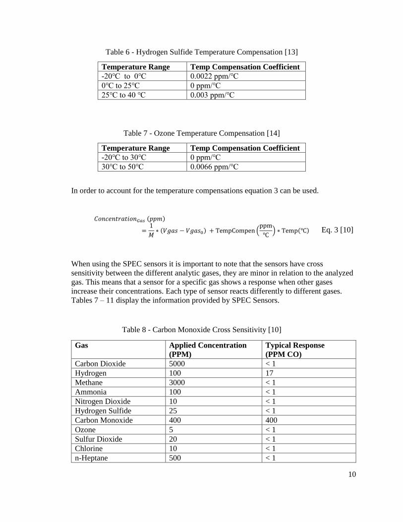
For this project we used the analog sensor modules (as seen on Figure 6) provided
by SPEC to use with their sensors (as seen on Figure 5). The analog sensor modules uses
two pairs of operational amplifiers to generate an output voltage that is proportional to
the concentration of the gas while maintaining the bias voltage to the sensor.
Figure 5 - SPEC Sensor
8
Figure 6 - SPEC Ultra Low Power Sensor Module (ULPSM)
The analog sensor modules operate at 3V and have under 45µW of power
consumption making them low power. These modules feature a temperature sensor and
allow for easy sensor replacement, in case of damage.
The gas concentration for each gas is calculated with Equation 1.
𝐶𝑜𝑛𝑐𝑒𝑛𝑡𝑟𝑎𝑡𝑖𝑜𝑛𝐺𝑎𝑠 (𝑝𝑝𝑚) =
1
𝑀∗ (𝑉𝑔𝑎𝑠 − 𝑉𝑔𝑎𝑠0) Eq. 1 [10]
Where concentration is measured in parts per million (ppm). Vgas is the output
voltage of the gas signal and Vgas0 is the output voltage of the gas signal in an
environment free of the target gas. M is the sensor calibration factor (V/ppm) and is
calculated in the following way:
𝑀 (
𝑉
𝑝𝑝𝑚) = 𝑆𝑒𝑛𝑠𝑖𝑡𝑖𝑣𝑖𝑡𝑦𝐶𝑜𝑑𝑒 (
𝑛𝐴
𝑝𝑝𝑚) ∗ 𝑇𝐼𝐴 𝐺𝑎𝑖𝑛 (
𝑘𝑉
𝐴) ∗ 10−9 (
𝐴
𝑛𝐴)
∗ 103 (𝑉
𝑘𝑉)
Eq. 2 [10]
Where the sensitivity code is printed on each sensor’s label. The TIA Gain is the
gain of the trans-impedance amplifier (TIA) of the analog sensor module. SPEC Sensors
provides different modules for the different analytic gases. The TIA Gain for each sensor
are provided by the manufacturer and are displayed on Table 2.

9
Table 2 - Trans-impedance Amplifier Gain [9]
Target Gas TIA Gain (kV/A)
Carbon Monoxide 100
Nitrogen Dioxide 499
Sulfur Dioxide 100
Hydrogen Sulfide 49.9
Ozone 499
The manufacturer of the sensors has registered that its sensor response have a
predictable fluctuation with changes in temperature. The sensor results must be adjusted
to account for the normal fluctuation. Tables 2 through 6 have Temperature coefficients
for each target gas.
Table 3 – Carbon Monoxide Temperature Compensation [10]
Temperature Range Temp Compensation Coefficient
-20℃ to 0℃ 0.06 ppm/℃
0℃ to 25℃ 0.3 ppm/℃
25℃ to 40 ℃ 1.4 ppm/℃
Table 4 – Nitrogen Dioxide Temperature Compensation [11]
Temperature Range Temp Compensation Coefficient
-20℃ to 30℃ 0 ppm/℃
30℃ to 50℃ 0.0066 ppm/℃
Table 5 – Sulfur Dioxide Temperature Compensation [12]
Temperature Range Temp Compensation Coefficient
-20℃ to 0℃ 0.012 ppm/℃
0℃ to 25℃ 0.056 ppm/℃
25℃ to 40 ℃ 0.46 ppm/℃
10
Table 6 - Hydrogen Sulfide Temperature Compensation [13]
Temperature Range Temp Compensation Coefficient
-20℃ to 0℃ 0.0022 ppm/℃
0℃ to 25℃ 0 ppm/℃
25℃ to 40 ℃ 0.003 ppm/℃
Table 7 - Ozone Temperature Compensation [14]
Temperature Range Temp Compensation Coefficient
-20℃ to 30℃ 0 ppm/℃
30℃ to 50℃ 0.0066 ppm/℃
In order to account for the temperature compensations equation 3 can be used.
𝐶𝑜𝑛𝑐𝑒𝑛𝑡𝑟𝑎𝑡𝑖𝑜𝑛𝐺𝑎𝑠 (𝑝𝑝𝑚)
=1
𝑀∗ (𝑉𝑔𝑎𝑠 − 𝑉𝑔𝑎𝑠0) + TempCompen (
ppm
℃) ∗ Temp(℃)
Eq. 3 [10]
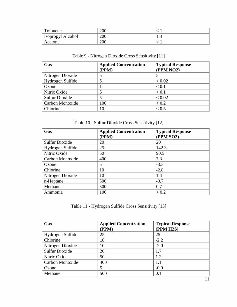
When using the SPEC sensors it is important to note that the sensors have cross
sensitivity between the different analytic gases, they are minor in relation to the analyzed
gas. This means that a sensor for a specific gas shows a response when other gases
increase their concentrations. Each type of sensor reacts differently to different gases.
Tables 7 – 11 display the information provided by SPEC Sensors.
Table 8 - Carbon Monoxide Cross Sensitivity [10]
Gas Applied Concentration
(PPM)
Typical Response
(PPM CO)
Carbon Dioxide 5000 < 1
Hydrogen 100 17
Methane 3000 < 1
Ammonia 100 < 1
Nitrogen Dioxide 10 < 1
Hydrogen Sulfide 25 < 1
Carbon Monoxide 400 400
Ozone 5 < 1
Sulfur Dioxide 20 < 1
Chlorine 10 < 1
n-Heptane 500 < 1
11
Tolouene 200 < 1
Isopropyl Alcohol 200 1.3
Acetone 200 < 1
Table 9 - Nitrogen Dioxide Cross Sensitivity [11]
Gas Applied Concentration
(PPM)
Typical Response
(PPM NO2)
Nitrogen Dioxide 5 5
Hydrogen Sulfide 5 < 0.02
Ozone 1 < 0.1
Nitric Oxide 5 < 0.1
Sulfur Dioxide 5 < 0.02
Carbon Monoxide 100 < 0.2
Chlorine 10 < 0.5
Table 10 - Sulfur Dioxide Cross Sensitivity [12]
Gas Applied Concentration
(PPM)
Typical Response
(PPM SO2)
Sulfur Dioxide 20 20
Hydrogen Sulfide 25 142.3
Nitric Oxide 50 90.5
Carbon Monoxide 400 7.3
Ozone 5 -3.3
Chlorine 10 -2.8
Nitrogen Dioxide 10 1.4
n-Heptane 500 -0.7
Methane 500 0.7
Ammonia 100 < 0.2
Table 11 - Hydrogen Sulfide Cross Sensitivity [13]
Gas Applied Concentration
(PPM)
Typical Response
(PPM H2S)
Hydrogen Sulfide 25 25
Chlorine 10 -2.2
Nitrogen Dioxide 10 -2.0
Sulfur Dioxide 20 1.7
Nitric Oxide 50 1.2
Carbon Monoxide 400 1.1
Ozone 5 -0.9
Methane 500 0.1
12
Ammonia 100 0.1
n-Heptane 500 < 0.05
Table 12 - Ozone Cross Sensitivity [14]
Gas Applied Concentration
(PPM)
Typical Response
(PPM O3)
Ozone 5 5
Hydrogen Sulfide 25 -5
Chlorine 10 10
Nitrogen Dioxide 5 5
n-Heptane 1000 < -0.1
Carbon Monoxide 400 < 0.05
Methane 500 < 0.05
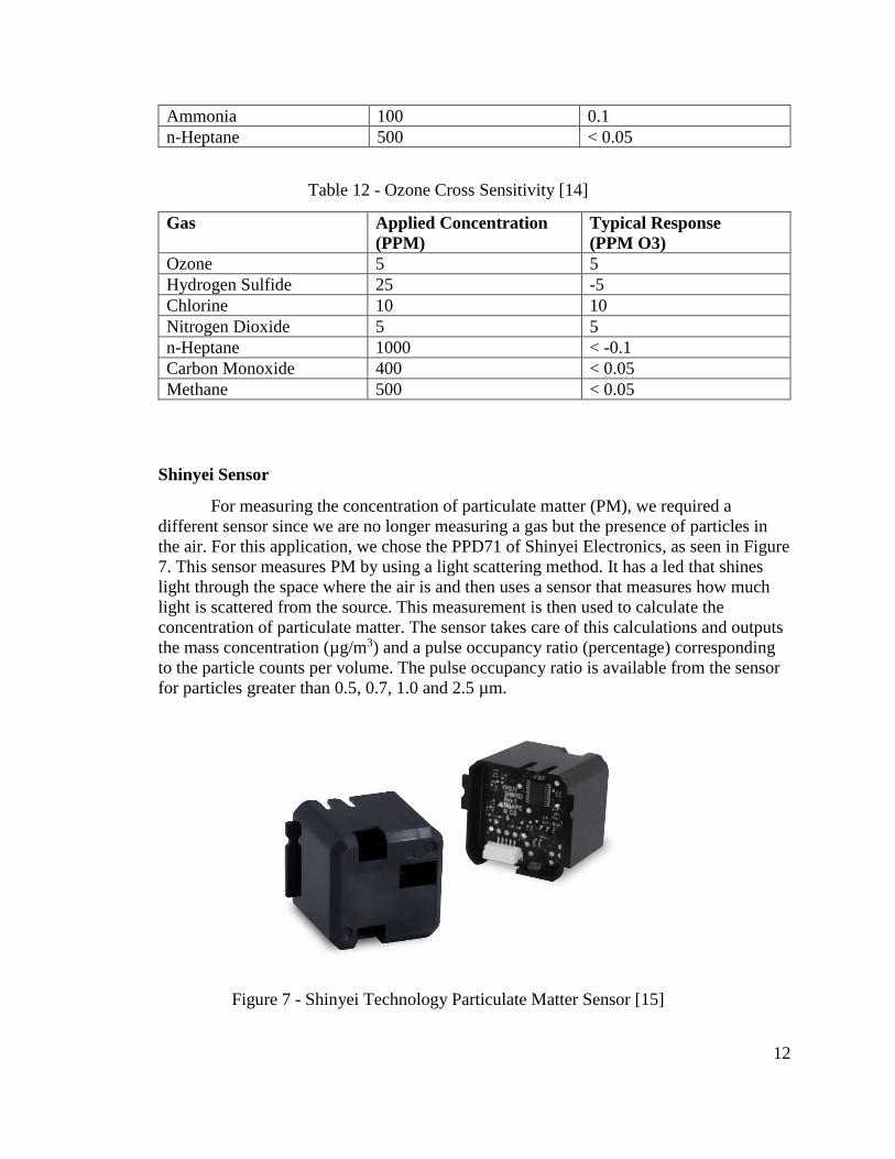
Shinyei Sensor
For measuring the concentration of particulate matter (PM), we required a
different sensor since we are no longer measuring a gas but the presence of particles in
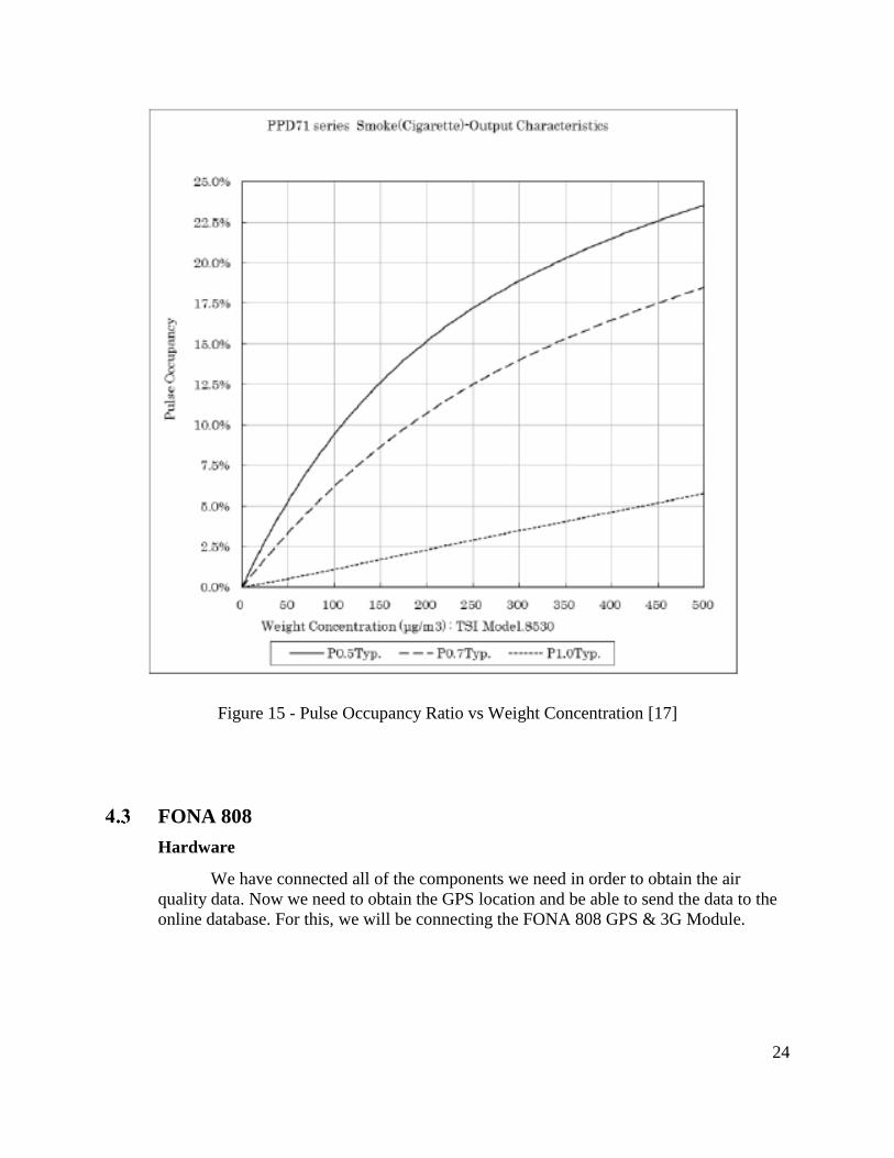
the air. For this application, we chose the PPD71 of Shinyei Electronics, as seen in Figure
7. This sensor measures PM by using a light scattering method. It has a led that shines
light through the space where the air is and then uses a sensor that measures how much
light is scattered from the source. This measurement is then used to calculate the
concentration of particulate matter. The sensor takes care of this calculations and outputs
the mass concentration (µg/m3) and a pulse occupancy ratio (percentage) corresponding
to the particle counts per volume. The pulse occupancy ratio is available from the sensor
for particles greater than 0.5, 0.7, 1.0 and 2.5 µm.
Figure 7 - Shinyei Technology Particulate Matter Sensor [15]
13
Wireless Data Transmission and GPS
Wireless data transmission is a key feature of this project. It will reduce the setup
time of the system and will allow the system to be mobile since no wired infrastructure is
needed. Also, since urban environments have a predominant and extensive cover of 3G
network. The system can be relocated easily if necessary. Note: the system is not
recommended to be used on moving vehicles as the gas concentrations can change faster
than the sensors are able to measure. Nonetheless, the system could be placed on a
moving vehicle and it can record data when the vehicle is stationary for longer periods.
In order to report the location of the data the integration of a Global Navigation
Satellite System (GNSS) capability into the system is required. GNSS or Global
Navigation Satellite System is a satellite system that is used to determine the location of a
specific device around the globe. A GNSS chip determines its location by receiving
signals from at least four different satellites and then computing the transmission delay of
the four satellites signals to determine the exact position on the globe.
There are four different GNSS constellations or satellite systems. There is Global
Positioning System (GPS), GLONASS, BeiDou and Galileo. GPS is the most widely
used system. It currently has 31 satellites orbiting earth. The GPS system is maintained
by the United States. On the other hand, GLONASS, translated to Global Navigation
Satellite System holds 23 satellites in operation and it is maintained by Russia. BeiDou is
the Chinese version; it is only operational in China’s region [16], although global
coverage is scheduled for 2020. Last, Galileo has not yet fully operational capability, and
changes to it are expected.
For our project the accuracy of GPS and GLONASS are practically the same.
GLONASS is especially better at extreme latitudes, far south and far north, due to the
position of its satellites. For this project, using GPS is sufficient.
For acquiring the GPS signal and and connecting to the cellular network we will
use the Adafruit FONA 808 3G and GPS breakout board. The FONA 808 is capable of
receiving and posting http requests as well as acquiring the GPS signal. This module is
also capable of making and receiving calls and text messages. In order to use this device
a 3G and GPS antenna are required. This module also requires a sim card and a dedicated
battery in order to operate.
Microcontroller
Last we need to select a microcontroller that can handle all of the requirements set
by the other components of the project. Each SPEC sensor require two analog inputs, we
have 5 sensors, and hence we need 10 analog inputs. It is also highly desirable that we
can use variable reference voltages to adjust the reference to obtain the highest accuracy
of the readings on the microcontroller. For the particulate matter sensor we require a
UART receiver on the microcontroller to receive the data. And for the FONA 808, 3G
and GPS module requires a UART receiver and a transmitter.

14
We also took into consideration the learning curve required to use the
microcontroller. We chose the ATmega2560 that is used on the Arduino Mega
development board since there is widely available documentation in its use.
The ATmega2560 is an 8-bit microcontroller that features 16 channel 10-bit ADC
(Analog to Digital Converter) channels. This means that the ATmega, although 8-bit can
access the 10 bit resolution in two operations. For our application we will left adjust the
reading and use 8-bit precision. The ATmega also has variable reference voltages
options. One can either use the default, set to 3.3V, or set VREF to 1.1V, 2.56V or to an
external reference voltage.
Solar Power and Battery
In order to develop the power system we worked with Kayleah Griffen to develop
a power system that could supply sufficient energy to our components. Please refer to
Appendix AAppendix A: Solar Power and Battery to find more information on the design
of this component.
The solar power system developed and found in Appendix A requires commands
from the microcontroller in order to function. The solar power system needs to connect to
a common ground, use I2C (SDA, SCL), a pulse with modulation(PWM) pin, an analog
input and must provide power to the power rail of the pollution system.
15
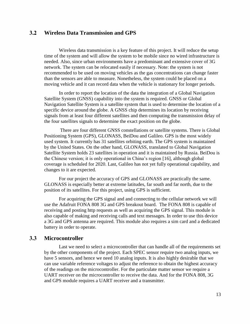
4. Implementation
Now that we have researched and selected the different components for the
project. Now, it is time to start the implementation. We will implement and write the
code for each component individually and then we will proceed to merge all of the
components into an integrated program. Figure 8 shows how the different components
interface with the ATmega2560 microcontroller.
Figure 8 – Overall System Signal Diagram
Electrochemical Sensors
Hardware
To start the implementation of the SPEC sensors we first need to understand the
physical layout of the SPEC Ultra-Low Power Analog Sensor Module (ULPSM) to
which the sensors are connected. Each ULPSM has a different internal wiring to
configure the different trans-impedance gains for the different sensors. However, they all
have the same configuration of outputs as seen on Figure 9. The descriptions of the pins
can be found on Table 13.

16
Figure 9 - SPEC ULPSM Layout
Table 13 – SPEC ULPSM Pin Descriptions [10]
PIN
Name
PIN
Num.
Type Description
Vgas 1 Output Proportional to the gas concentration
Vref 2 Output Reference voltage. Equivalent to zero for
Vgas. Note: It must be connected to a buffer
amplifier as it has a high impedance output
Vtemp 3 Output Proportional to the temperature
SCL 4 Not used
SDA 5 Not used
GND 6 Input Universal Ground for power and signal
Vreg 7 Input Supply Voltage 2.7V to 3.3V
V+ 8 Input Supply Voltage 2.7V to 3.3V
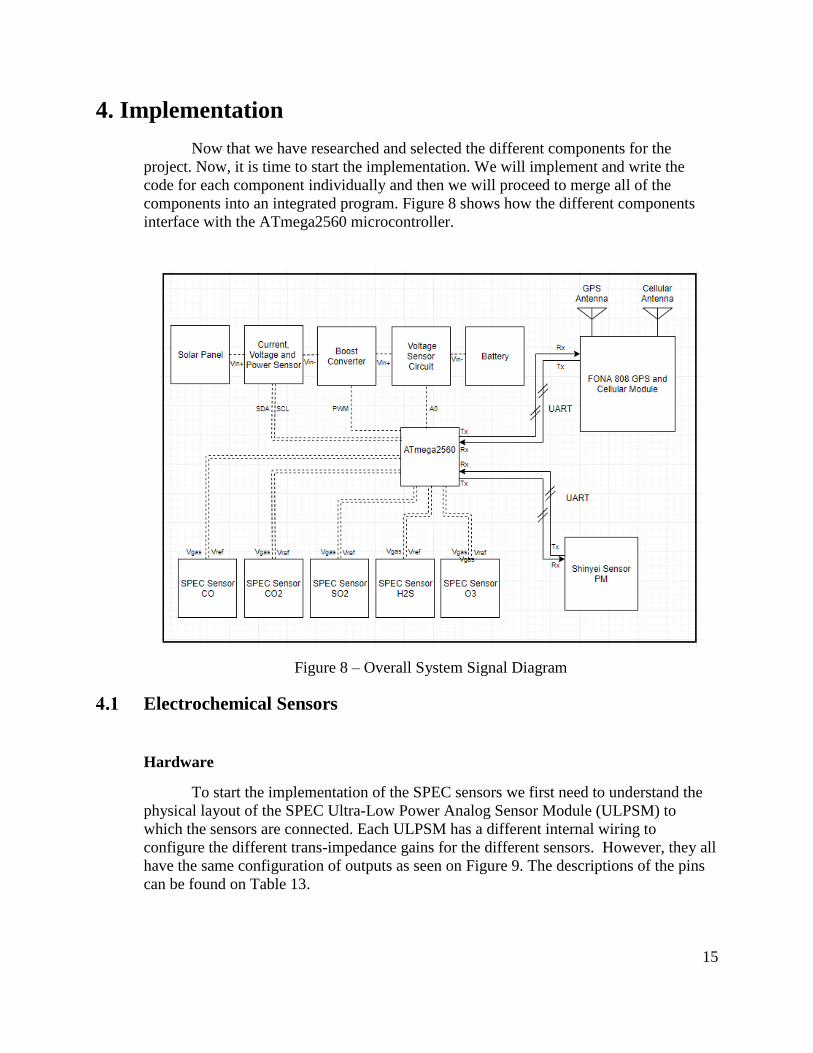
The ULPSM are powered throught the 3V rail. Note than pins 8 & 9 can both power the system.
Connecting only one is sufficient. Vref is connected to a buffer amplifier as seen on Figure 10.
Next, we will assign the outputs Vref and Vgas pins to the ATmega pins. Please refer toTable 14.
Please note that we use the Temp connection of the Ozone ULPSM only as we assume that the
temperature measured there will be an accurate representation of the temperature around all other
sensors. Later we will show the development of a PCB board with the Atmega 2560
microcontroller so the last column pin numbers in Table 14 become relevant.
17
Figure 10 - Spec Sensor Connection to Buffer Amplifier
Table 14 - SPEC Sensor Pin Assignments
Gas ULPSM Pin Arduino
Label
Arduino
Mega Pins
Atmega 2560 pins
(Custom PCB)
Carbon
Monoxide
Vref A0 54 55
Vgas
(Buffer out)
A1 55 54
Nitrogen
Dioxide
Vref A2 56 57
Vgas
(Buffer out)
A3 57 56
Sulfur
Dioxide
Vref A4 58 59
Vgas
(Buffer out)
A5 59 58
Hydrogen
Sulfide
Vref A6 60 61
Vgas
(Buffer out)
A7 61 60
Ozone Vref A8 62 63
Vgas A9 63 62
Vtemp
(Buffer out)
A10 64 64
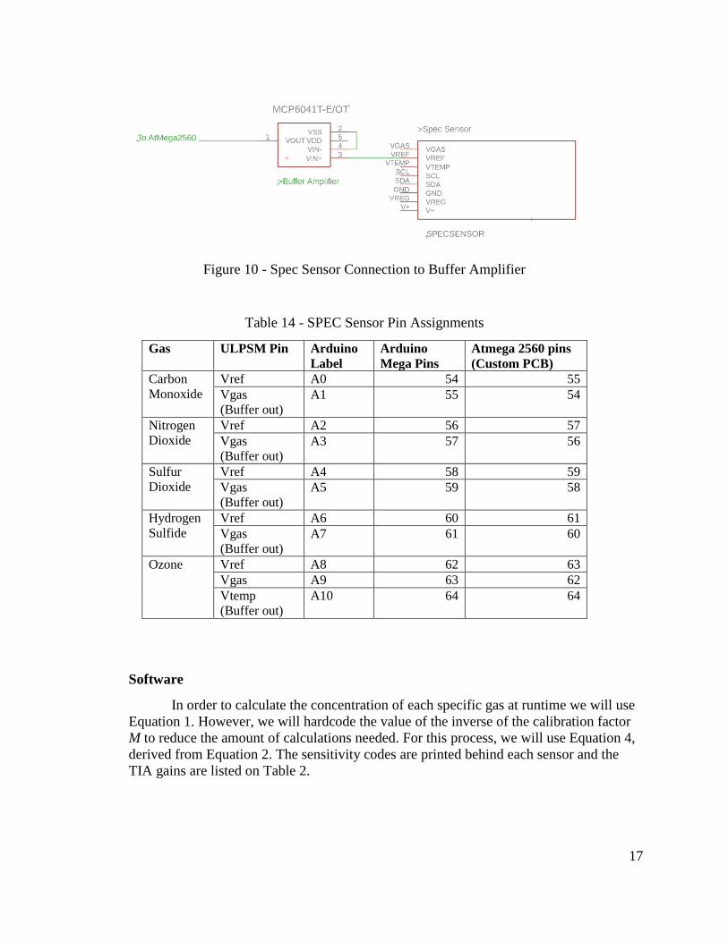
Software
In order to calculate the concentration of each specific gas at runtime we will use
Equation 1. However, we will hardcode the value of the inverse of the calibration factor
M to reduce the amount of calculations needed. For this process, we will use Equation 4,
derived from Equation 2. The sensitivity codes are printed behind each sensor and the
TIA gains are listed on Table 2.
18
𝑀𝑋−1 (
𝑝𝑝𝑚
𝑉)
=1
𝑆𝑒𝑛𝑠𝑖𝑡𝑖𝑣𝑖𝑡𝑦𝐶𝑜𝑑𝑒 (𝑛𝐴
𝑝𝑝𝑚) ∗ 𝑇𝐼𝐴 𝐺𝑎𝑖𝑛 (𝑘𝑉𝐴 ) ∗ 10−9 (
𝐴𝑛𝐴) ∗ 103 (
𝑉𝑘𝑉
)
Eq. 4
In our system implementation, the following is the result of the inverse calibration
factors. Please note that the Sensitivity codes will change with every sensor.
Table 15 - Results of the Inverse Calibration Factor
Analytic Gas Sensitivity
Code
TIA
GAIN
1/M
(ppm/V)
Carbon
Monoxide 4.44 100 2252.252
Nitrogen
Dioxide -23.81 49.9 -841.667
Sulfur
Dioxide 36.58 499 54.784
Hydrogen
Sulfide -267.86 100 -37.333
Ozone -72.04 499 -27.818
In the header file in the code we have hardcoded the results of Table 15 for each
sensor under the names SPEC_CONSTANT_1_M_[GAS]. Where [GAS] is replaced by
the chemical notation for each of the compounds. This can be found in the ‘mqpdef.h’
file.
19
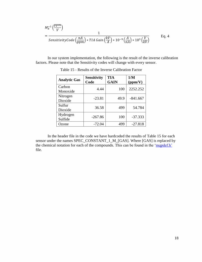
Figure 11 - ULPSM Vgas and Vref Output
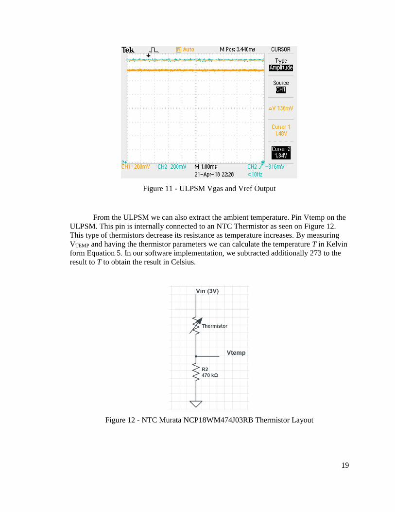
From the ULPSM we can also extract the ambient temperature. Pin Vtemp on the
ULPSM. This pin is internally connected to an NTC Thermistor as seen on Figure 12.
This type of thermistors decrease its resistance as temperature increases. By measuring
VTEMP and having the thermistor parameters we can calculate the temperature T in Kelvin
form Equation 5. In our software implementation, we subtracted additionally 273 to the
result to T to obtain the result in Celsius.
Figure 12 - NTC Murata NCP18WM474J03RB Thermistor Layout
20
Table 16 - Thermistor
NTC Thermistor Values
BCoefficient 4600
T0 298[ ̊K]
Vin 3 [V]
1
𝑇=
1
𝑇0+
1
𝐵ln (
𝑉𝑖𝑛
𝑉𝑇𝐸𝑀𝑃 − 1)
Eq. 5
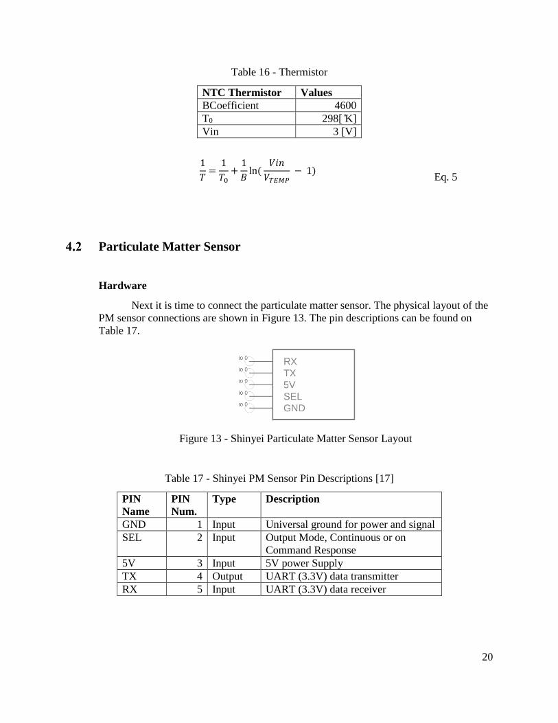
Particulate Matter Sensor
Hardware
Next it is time to connect the particulate matter sensor. The physical layout of the
PM sensor connections are shown in Figure 13. The pin descriptions can be found on
Table 17.
Figure 13 - Shinyei Particulate Matter Sensor Layout
Table 17 - Shinyei PM Sensor Pin Descriptions [17]
PIN
Name
PIN
Num.
Type Description
GND 1 Input Universal ground for power and signal
SEL 2 Input Output Mode, Continuous or on
Command Response
5V 3 Input 5V power Supply
TX 4 Output UART (3.3V) data transmitter
RX 5 Input UART (3.3V) data receiver
21
The 5V pin is connected to the 5V rail, GND is connected to the universal ground
of the system, SEL is connected to ground and TX is connected to the ATmega Pin as
seen on Table 18. Note that the RX pin on the Shinyei PM sensor is not connected.
Table 18 - Shinyei PM Sensor Pin Assignments
Shinyei PM
Sensor Pins
Arduino Label Arduino
Mega Pin
Atmega 2560 pins
(Custom PCB)
TX RX3 15 63
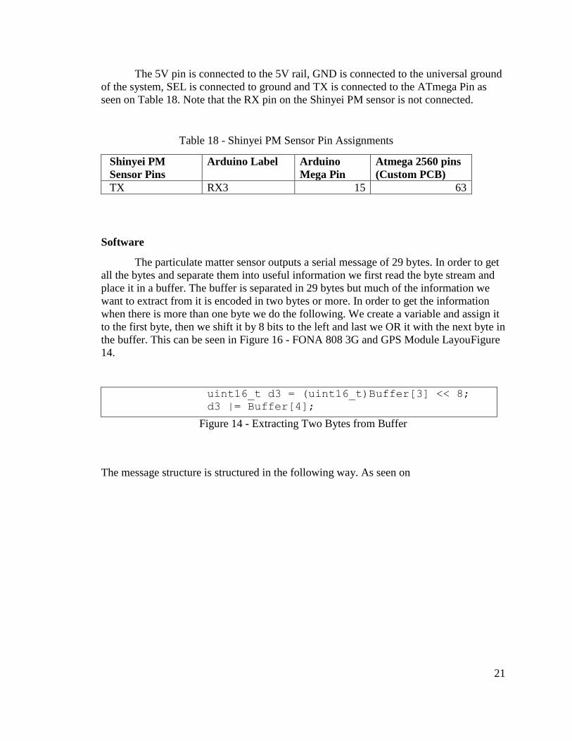
Software
The particulate matter sensor outputs a serial message of 29 bytes. In order to get
all the bytes and separate them into useful information we first read the byte stream and
place it in a buffer. The buffer is separated in 29 bytes but much of the information we
want to extract from it is encoded in two bytes or more. In order to get the information
when there is more than one byte we do the following. We create a variable and assign it
to the first byte, then we shift it by 8 bits to the left and last we OR it with the next byte in
the buffer. This can be seen in Figure 16 - FONA 808 3G and GPS Module LayouFigure
14.
uint16_t d3 = (uint16_t)Buffer[3] << 8;
d3 |= Buffer[4];
Figure 14 - Extracting Two Bytes from Buffer
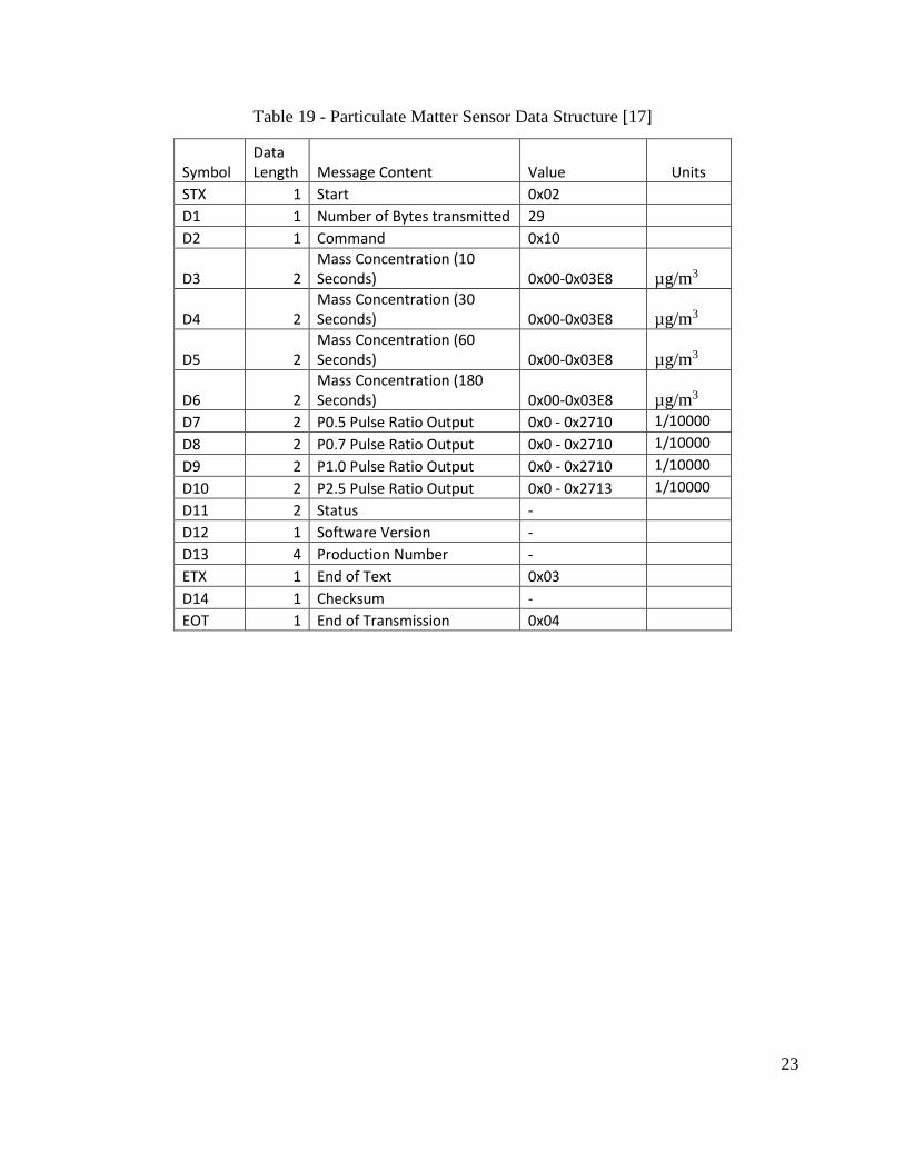
The message structure is structured in the following way. As seen on

22
Table 19. The mass concentrations of data D3 – D6 is measured in µg/m3. D7 – D10 is
measured as the occupancy ratio of particles greater than the specified value.
23
Table 19 - Particulate Matter Sensor Data Structure [17]
Symbol Data Length Message Content Value Units
STX 1 Start 0x02
D1 1 Number of Bytes transmitted 29
D2 1 Command 0x10
D3 2 Mass Concentration (10 Seconds) 0x00-0x03E8 µg/m3
D4 2 Mass Concentration (30 Seconds) 0x00-0x03E8 µg/m3
D5 2 Mass Concentration (60 Seconds) 0x00-0x03E8 µg/m3
D6 2 Mass Concentration (180 Seconds) 0x00-0x03E8 µg/m3
D7 2 P0.5 Pulse Ratio Output 0x0 - 0x2710 1/10000
D8 2 P0.7 Pulse Ratio Output 0x0 - 0x2710 1/10000
D9 2 P1.0 Pulse Ratio Output 0x0 - 0x2710 1/10000
D10 2 P2.5 Pulse Ratio Output 0x0 - 0x2713 1/10000
D11 2 Status -
D12 1 Software Version -
D13 4 Production Number -
ETX 1 End of Text 0x03
D14 1 Checksum -
EOT 1 End of Transmission 0x04
24
Figure 15 - Pulse Occupancy Ratio vs Weight Concentration [17]
FONA 808
Hardware
We have connected all of the components we need in order to obtain the air
quality data. Now we need to obtain the GPS location and be able to send the data to the
online database. For this, we will be connecting the FONA 808 GPS & 3G Module.
25
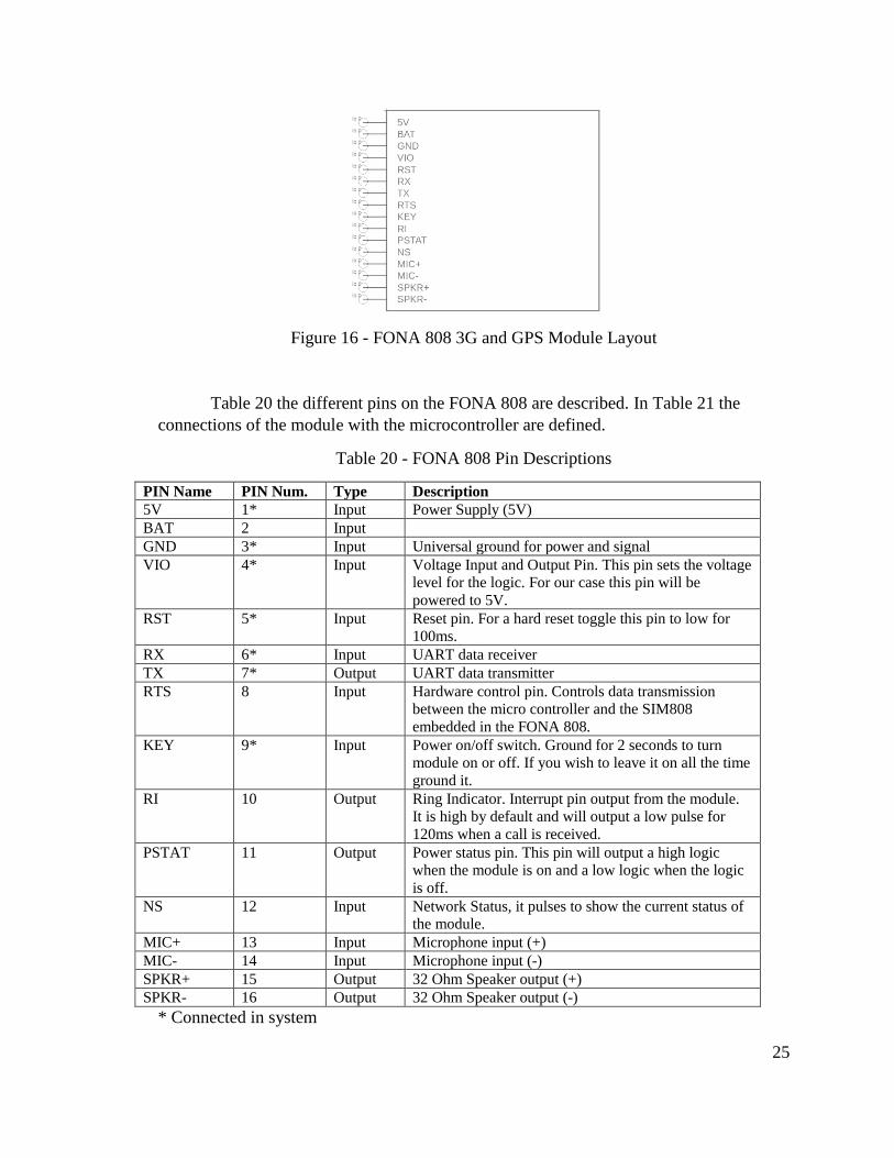
Figure 16 - FONA 808 3G and GPS Module Layout
Table 20 the different pins on the FONA 808 are described. In Table 21 the
connections of the module with the microcontroller are defined.
Table 20 - FONA 808 Pin Descriptions
PIN Name PIN Num. Type Description
5V 1* Input Power Supply (5V)
BAT 2 Input
GND 3* Input Universal ground for power and signal
VIO 4* Input Voltage Input and Output Pin. This pin sets the voltage
level for the logic. For our case this pin will be
powered to 5V.
RST 5* Input Reset pin. For a hard reset toggle this pin to low for
100ms.
RX 6* Input UART data receiver
TX 7* Output UART data transmitter
RTS 8 Input Hardware control pin. Controls data transmission
between the micro controller and the SIM808
embedded in the FONA 808.
KEY 9* Input Power on/off switch. Ground for 2 seconds to turn
module on or off. If you wish to leave it on all the time
ground it.
RI 10 Output Ring Indicator. Interrupt pin output from the module.
It is high by default and will output a low pulse for
120ms when a call is received.
PSTAT 11 Output Power status pin. This pin will output a high logic
when the module is on and a low logic when the logic
is off.
NS 12 Input Network Status, it pulses to show the current status of
the module.
MIC+ 13 Input Microphone input (+)
MIC- 14 Input Microphone input (-)
SPKR+ 15 Output 32 Ohm Speaker output (+)
SPKR- 16 Output 32 Ohm Speaker output (-)
* Connected in system
26
Table 21 - FONA Module Pin Assignments
FONA 808
Arduino Label Arduino Mega Pin Atmega 2560
pins(Custom PCB)
RST PWM 4 4 1
RX PWM 2 2 23
TX PWM 10 10 6
Software
The data that is collected from our system will be sent to a data base server,
namely Ubidots. Ubidots is compatible with the FONA 808 module as it features a
comprehensible library to communicate with the device [18]. Ubidots is an online
platform that provides hosting of data points, intuitive visualizations and provides basic
analysis tools.
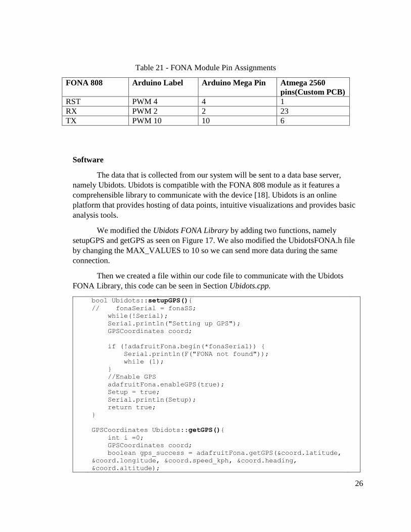
We modified the Ubidots FONA Library by adding two functions, namely
setupGPS and getGPS as seen on Figure 17. We also modified the UbidotsFONA.h file
by changing the MAX_VALUES to 10 so we can send more data during the same
connection.
Then we created a file within our code file to communicate with the Ubidots
FONA Library, this code can be seen in Section Ubidots.cpp.
bool Ubidots::setupGPS(){
// fonaSerial = fonaSS;
while(!Serial);
Serial.println("Setting up GPS");
GPSCoordinates coord;
if (!adafruitFona.begin(*fonaSerial)) {
Serial.println(F("FONA not found"));
while (1);
}
//Enable GPS
adafruitFona.enableGPS(true);
Setup = true;
Serial.println(Setup);
return true;
}
GPSCoordinates Ubidots::getGPS(){
int i =0;
GPSCoordinates coord;
boolean gps_success = adafruitFona.getGPS(&coord.latitude,
&coord.longitude, &coord.speed_kph, &coord.heading,
&coord.altitude);

27
if (gps_success) {
Serial.println(coord.latitude);
return coord;
}
coord.latitude = 200.123456;
coord.longitude= -200.654321;
return coord;
}
Figure 17 - UbidotsFONA Modifications for GPS Acquisition
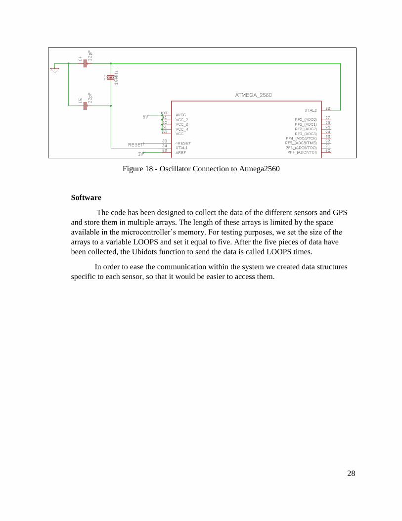
Atmega 2560
Hardware
In order to program the Atmega 2560 we used an external Arduino as an In-
Circuit Serial Programmer (ISP). For this specific task, we allotted six pins to be used as
seen on Table 22 - Programming Pins Atmega2560Table 22. In addition to leaving this
pins connected to female headers to connect the programmer we need to connect a
16Mhz Oscillator between pins XTAL1 and XTAL2 of the Atmega2560 and with a 22pF
capacitor between XTAL1 and GND and another 22pF capacitor between XTAL2 and
GND as seen on Figure 18.
Table 22 - Programming Pins Atmega2560
Name Atmega2560 Arduino Uno
Reset 30 10
MOSI 21 11
MISO 22 12
SCK 20 13
GND GND GND
5V VCC VCC
28
Figure 18 - Oscillator Connection to Atmega2560
Software
The code has been designed to collect the data of the different sensors and GPS
and store them in multiple arrays. The length of these arrays is limited by the space
available in the microcontroller’s memory. For testing purposes, we set the size of the
arrays to a variable LOOPS and set it equal to five. After the five pieces of data have
been collected, the Ubidots function to send the data is called LOOPS times.
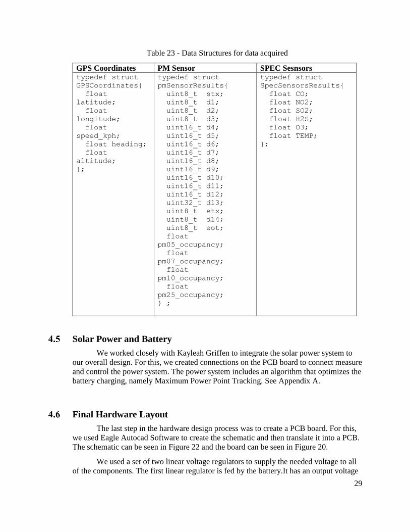
In order to ease the communication within the system we created data structures
specific to each sensor, so that it would be easier to access them.
29
Table 23 - Data Structures for data acquired
GPS Coordinates PM Sensor SPEC Sesnsors typedef struct
GPSCoordinates{
float
latitude;
float
longitude;
float
speed_kph;
float heading;
float
altitude;
};
typedef struct
pmSensorResults{
uint8_t stx;
uint8_t d1;
uint8_t d2;
uint8_t d3;
uint16_t d4;
uint16_t d5;
uint16_t d6;
uint16_t d7;
uint16_t d8;
uint16_t d9;
uint16_t d10;
uint16_t d11;
uint16_t d12;
uint32_t d13;
uint8_t etx;
uint8_t d14;
uint8_t eot;
float
pm05_occupancy;
float
pm07_occupancy;
float
pm10_occupancy;
float
pm25_occupancy;
} ;
typedef struct
SpecSensorsResults{
float CO;
float NO2;
float SO2;
float H2S;
float O3;
float TEMP;
};
Solar Power and Battery
We worked closely with Kayleah Griffen to integrate the solar power system to
our overall design. For this, we created connections on the PCB board to connect measure
and control the power system. The power system includes an algorithm that optimizes the
battery charging, namely Maximum Power Point Tracking. See Appendix A.
Final Hardware Layout
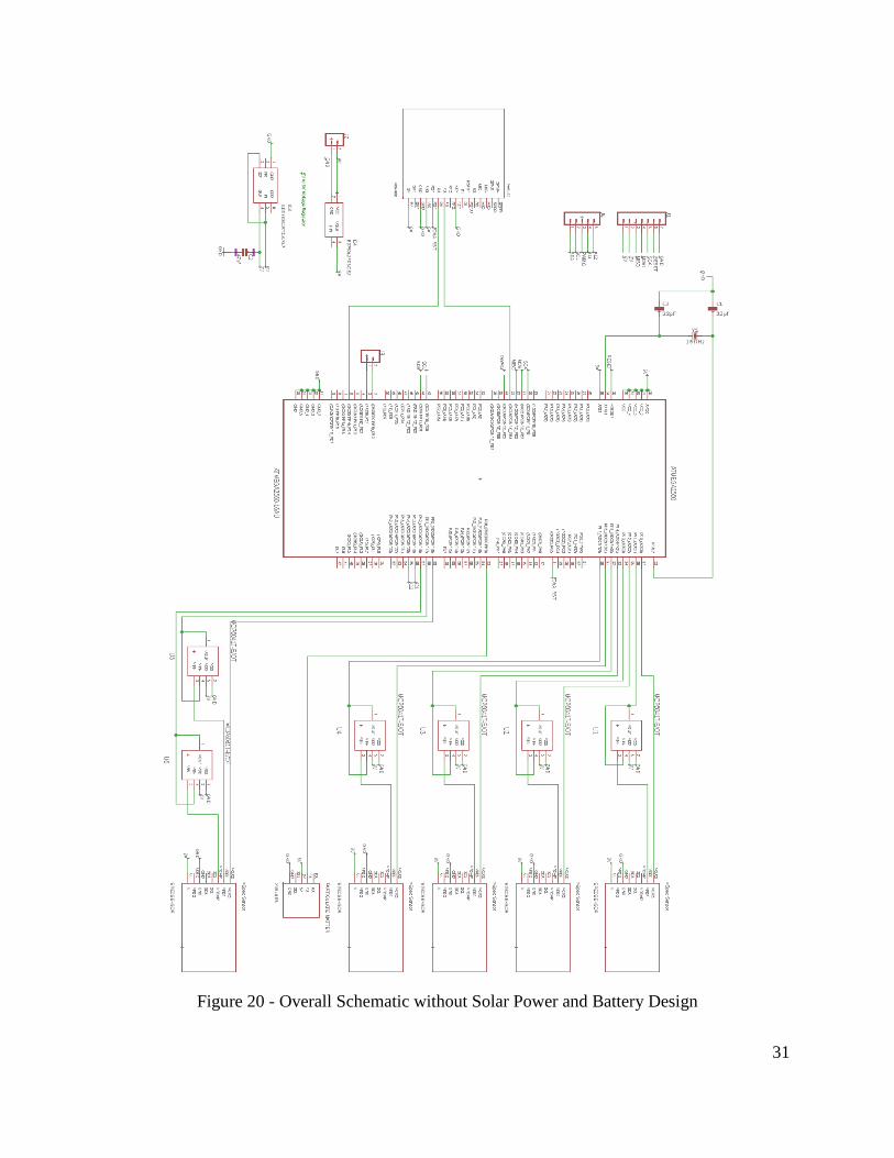
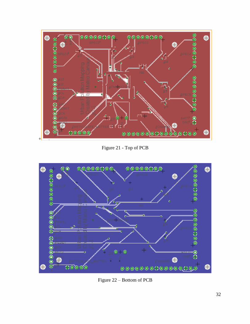
The last step in the hardware design process was to create a PCB board. For this,
we used Eagle Autocad Software to create the schematic and then translate it into a PCB.
The schematic can be seen in Figure 22 and the board can be seen in Figure 20.
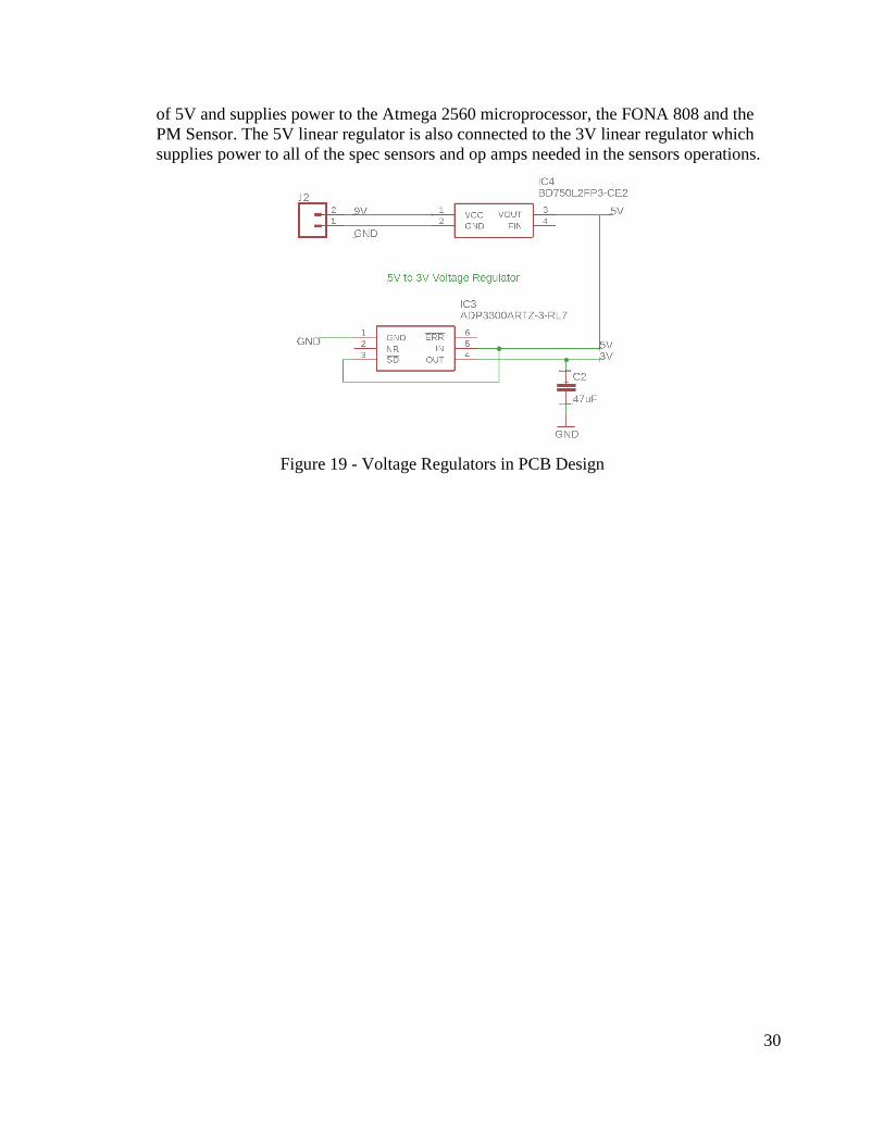
We used a set of two linear voltage regulators to supply the needed voltage to all
of the components. The first linear regulator is fed by the battery.It has an output voltage
30
of 5V and supplies power to the Atmega 2560 microprocessor, the FONA 808 and the
PM Sensor. The 5V linear regulator is also connected to the 3V linear regulator which
supplies power to all of the spec sensors and op amps needed in the sensors operations.
Figure 19 - Voltage Regulators in PCB Design
31
Figure 20 - Overall Schematic without Solar Power and Battery Design
32
+
Figure 21 - Top of PCB
Figure 22 – Bottom of PCB

33
5. Results
Throughout our project, we were able to test the functionality of the different
components. In this section, we describe the challenges and results we faced while trying
to obtain the data.
Our main goal of developing a prototype with extensive functionalities has been
achieved. The prototype sits on a custom PCB able to measure five different gases,
monitor particulate matter, record the GPS location, transmit the data to an online server
and power itself using solar power.
First off, we tested our temperature sensor response. Having the temperature on
hand is extremely important while running data analysis on the different gases since the
SPEC sensors require different adjustments with different temperatures. In Figure 23 the
temperature remains constant just under 25℃ until second 48 where we grab the sensor
with the hand to increase the temperature. Then at second 65, we let go of the sensor. As
you can see the sensor responds appropriately to a sudden change in the environment and
takes a longer a period of time to cool down.
Figure 23 - Temperature Sensor Results
0
5
10
15
20
25
30
35
1 5 9
13
17
21
25
29
33
37
41
45
49
53
57
61
65
69
73
77
81
85
89
93
97
10
1
10
5
Tem
per
atu
re (
℃)
Time (s)
Temperature vs Time

34
We also tested the connection of the PM sensor to verify we were getting the correct data sent by
the PM module. For this we compared the values we expected (

35
Table 19) with the experimental results (Figure 24). All of the fixed values match.
Figure 24 - Results from PM Sensor Message
Next, we tested the GPS coordinates response. The results obtained can be seen in
Figure 25. Where “42.268302” is the latitude and “-71.804400” is the longitude. This
coordinates match precisely to where the device was located for the measurement.
Figure 25 - GPS Response
36
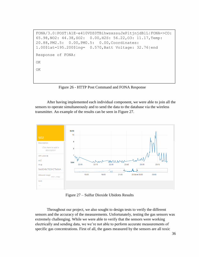
Figure 26 - HTTP Post Command and FONA Response
After having implemented each individual component, we were able to join all the
sensors to operate simultaneously and to send the data to the database via the wireless
transmitter. An example of the results can be seen in Figure 27.
Figure 27 – Sulfur Dioxide Ubidots Results
Throughout our project, we also sought to design tests to verify the different
sensors and the accuracy of the measurements. Unfortunately, testing the gas sensors was
extremely challenging. While we were able to verify that the sensors were working
electrically and sending data, we we’re not able to perform accurate measurements of
specific gas concentrations. First of all, the gases measured by the sensors are all toxic
FONA/3.0|POST|A1E-e410VDZ0TBihwsxssuJxPltjnjdBlL|FONA=>CO:
65.98,NO2: 44.38,SO2: 0.00,H2S: 56.22,O3: 11.17,Temp:
20.88,PM2.5: 0.00,PM0.5: 0.00,Coordinates:
1.00$lat=195.200$lng= 0.570,Batt Voltage: 32.76|end
Response of FONA:
OK
OK
37
and acquiring test samples was difficult. Also, the SPEC sensors have a prolonged
reaction time of ~2min. Controlling the space around the sensors was extremely
challenging. In addition to this we had no enclosed facilities designed to test gas
concentrations, so the experiments we conducted to measure specific gases returned no
valuable data points.
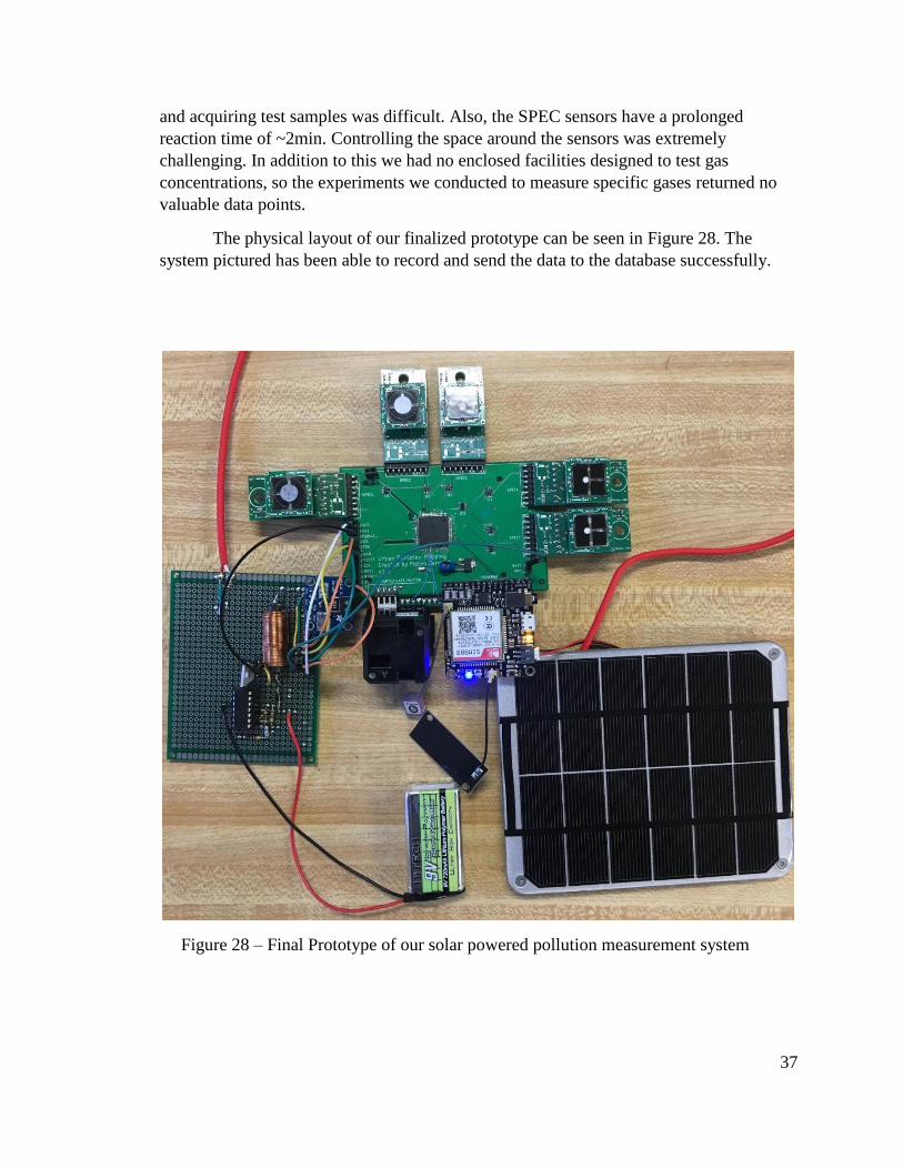
The physical layout of our finalized prototype can be seen in Figure 28. The
system pictured has been able to record and send the data to the database successfully.
Figure 28 – Final Prototype of our solar powered pollution measurement system

38
6. Conclusion and Recommendations
Air pollution in urban environments represents a grave risk to human health and
well-being. Collecting air pollution data has the potential to become an important tool in
an urban planner’s hands to make better and effective changes to reduce the harmful
gases. It can also have many uses if the data is available to the public, especially in
creating awareness and fueling advocacy.
Regarding this project, most importantly, we successfully developed a prototype
to monitor the six main air pollutants that threaten health in our cities. The prototype
calculates the levels of the pollutants and wirelessly transmits the data to an online
database. In addition to this we have created a self-sufficient power system that powers
itself from sun light and charges a battery when there is adequate lighting. When the
photovoltaic cells are not active, the battery supplies power to the system.
The objective of creating a prototype that would monitor and report air quality to
an online database while harvesting its energy from its surrounding has been achieved.
Nevertheless, considerable more work needs to occur in order to create a comprehensive
device that can reliably provide air quality data over long periods. We also recommend
conducting a detailed analysis of the SPEC sensors. Unfortunately, the available data
from and reviews of the SPEC sensors are very limited. However, we have been told,
informally, by experts in the field that the sensors can be sensitive to humidity. If this
system were to be used on a large scale throughout cities, an investigation on the
accuracy of the SPEC sensors over a variety of meteorological conditions must be made
to ensure the data gathered is accurate under all conditions.
Air quality is not uniform and can change rapidly due to many factors, we
recommend that the system be equipped with machine learning and artificial intelligence
algorithms to better predict the levels of pollutants and create more comprehensive
pollutant maps.
39
7. Bibliography
[1] World Health Organization, "Ambient air pollution: A global assessment of exposure and
burden of disease," 2016.
[2] M. Brauer, "Ambient Air Pollution Exposure Estimation for the Global Burden of Disease
2013," Enivronmental Science & Technology, pp. 79-88, 2015.
[3] OECD, "OECD Environmental Outlook to 2050: The Consequences of Inaction.,"
Publishing, Paris, 2012.
[4] EPA, "Latest Findings on National Air Quality," United States Environmental Protection
Agency, 2008.
[5] World Health Organization, "Health Aspects of Air Pollution with Particulate Matter,
Ozone and Nitrogen Dioxide," Bonn, Germany, 2003.
[6] United States Department of Labor (OSHA), "Hydrogen Sulfide," [Online]. Available:
https://www.osha.gov/SLTC/hydrogensulfide/hazards.html. [Accessed 2018].
[7] Luft Hamburg , "Luftmessstation Hamburg-Stresemannstraße," [Online]. Available:
http://luft.hamburg.de/messstationen-liste/4244982/17sm-stresemannstrasse.html.
[Accessed April 2018].
[8] A. Carvajal, Hamburg Air Quality Monitoring Station, Hamburg, 2018.
[9] SPEC Sensors, SPEC Sensor Operation Overview, May 2016.
[10] SPEC Sensors, "Ultra-Low Power Analog Sensor Module for Carbon Monoxide" ULPSM-
CO 968-001 Datasheet, October 2016.
[11] SPEC Sensors, "Ultra-Low Power Analog Sensor Module for Nitrogen Dioxide" ULPSM-
NO2 968-047 Datasheet, August 2017.
[12] SPEC Sensors, "Ultra-Low Power Analog Sensor Module for Sulfur Dioxide" ULPSM-
SO2 968-006 Datasheet, October 2016.
[13] SPEC Sensors, "Ultra-Low Power Analog Sensor Module for Hydrogen Sulfide" ULPSM-
H2S 968-003 Datasheet, October 2016.
[14] SPEC Sensors, "Ultra-Low Power Analog Sensor Module for Ozone" ULPSM-03 968-046
Datasheet, August 2017.
40
[15] Shinyei Technology, "PPD 71 Particle Sensor Unit," [Online]. Available:
http://www.shinyei.co.jp/stc/eng/optical/main_ppd71.html. [Accessed January 2018].
[16] Novatel, "Chapter 3 GNSS Satellite Systems," [Online]. Available:
https://www.novatel.com/an-introduction-to-gnss/chapter-3-satellite-systems/beidou/.
[Accessed March 2018].
[17] Shinyei Technology CO., "Particulate Matter Sensor" PPD71 Datasheet, August, 2017.
[18] Ubidots, "Ubidots FONA Library," 2016. [Online]. Available:
https://github.com/ubidots/Ubidots-FONA. [Accessed March 2018].
[19] N. Mohan, T. Undeland and W. P. Robbins, Power electronics: Converters, applications,
and design (3rd ed.), Hoboken, NJ: John Wiley & Sons, 2003.
[20] N. Notman, "Chemistry World," 12 January 2017. [Online]. Available:
https://www.chemistryworld.com/feature/urban-air-pollution/2500224.article.
[21] M. L. Melamed, T. Zhu and L. Jalkanen, "Urban Air Pollution: a new look to an old
problem," IGBP's Global Change Magazine, 2013.
[22] T. Zhu, M. L. Melamed, D. Parrish, M. Gauss, L. Gallardo Klenner, M. Lawrence, A.
Konare and C. Liousse, "Impacts of Megacities on Air Pollution and Climate," 2012.
[23] EPA, "Basic Information about NO2," [Online]. Available: https://www.epa.gov/no2-
pollution/basic-information-about-no2#Effects.
[24] Diodes Incorporated, 1N5817 - 1N5819 1.0A Schottky Barrier Rectifier [Data Sheet],
April, 2018.
[25] GN Batteries and Electronics, Inc, RLI-9720 Li-Ion Polymer Battery Pack [Data Sheet],
2011.
[26] International Rectifier, IRL2703 HEXFET Power MOSFET [Data Sheet].
[27] Microchip, MCP6041/2/3/4 Op Amp Datasheet, 2013.
[28] Texas Instruments, Zero Drift, Bi-Directional Current/Power Monitor with I2C Interface
[Data Sheet], 2011.
[29] Voltaic Systems, 2W 6V 112x136 mm Solar Panel [Data Sheet], 2017.
[30] Voltaic Systems, "Small Solar Panels," [Online]. Available:
https://www.voltaicsystems.com/solar-panels. [Accessed 24 04 2018].

41
[31] N. Femia, G. Petrone and M. Vitelli, Power electronics and control techniques for
maximum energy harvesting in photovoltaic systems, CRC Press, 2013.
[32] Y. Mahmoud, W. Ziao and H. H. Zeineldin, "A parameterization approach for enhancing
PV model accuracy," IEEE Transactions on Industrial Electronics, 2013.

42
8. Appendix
Appendix A: Solar Power and Battery
Solar Power Design
This chapter of the report, written by Kayleah Griffen, provides auxiliary material
developed by Kayleah Griffen to do more in depth ECE work for the fulfillment of her
second degree. The work presented in this chapter complements the MQP of Mateo
Carvajal: Mapping Urban Pollution. Mateo Carvajal’s MQP can be separately referenced
for additional context on urban pollution. The purpose of the work described in this
chapter is to provide the power system for the urban pollution mapping system. By using
solar energy charging the urban pollution mapping system would be able to be self-
sufficient in terms of power and therefor operate independently without service for longer
periods of time. Based on the power consumption of the system and the microcontroller
selected, a solar panel, battery, and a boost converter were chosen for the system. The
power generation system implemented used a maximum power point tracking algorithm
in order for it to harvest the most energy from the solar panel to maximize the use of the
solar panel. The components selected in this project were the solar panel, battery,
inductor, MOSFET, diode, as well as the voltage and current sensing subsystems. The
Practical Model of the solar panel was modeled in MATLAB and the entire charging
system was modeled in Simulink prior to actually building the system. Simulation
allowed for more informed decisions about the sizes of certain components as well as to
better understand the system behavior. After the system was designed, simulated and
modified it was constructed and tested.
43
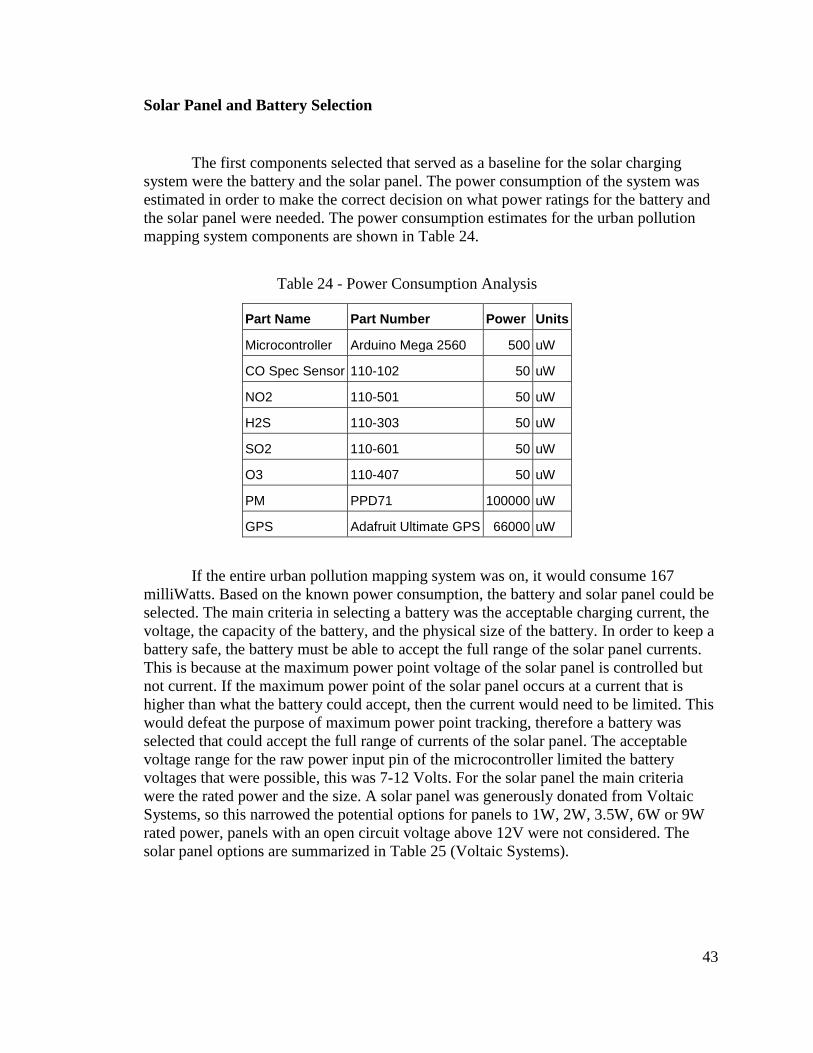
Solar Panel and Battery Selection
The first components selected that served as a baseline for the solar charging
system were the battery and the solar panel. The power consumption of the system was
estimated in order to make the correct decision on what power ratings for the battery and
the solar panel were needed. The power consumption estimates for the urban pollution
mapping system components are shown in Table 24.
Table 24 - Power Consumption Analysis
Part Name Part Number Power Units
Microcontroller Arduino Mega 2560 500 uW
CO Spec Sensor 110-102 50 uW
NO2 110-501 50 uW
H2S 110-303 50 uW
SO2 110-601 50 uW
O3 110-407 50 uW
PM PPD71 100000 uW
GPS Adafruit Ultimate GPS 66000 uW
If the entire urban pollution mapping system was on, it would consume 167
milliWatts. Based on the known power consumption, the battery and solar panel could be
selected. The main criteria in selecting a battery was the acceptable charging current, the
voltage, the capacity of the battery, and the physical size of the battery. In order to keep a
battery safe, the battery must be able to accept the full range of the solar panel currents.
This is because at the maximum power point voltage of the solar panel is controlled but
not current. If the maximum power point of the solar panel occurs at a current that is
higher than what the battery could accept, then the current would need to be limited. This
would defeat the purpose of maximum power point tracking, therefore a battery was
selected that could accept the full range of currents of the solar panel. The acceptable
voltage range for the raw power input pin of the microcontroller limited the battery
voltages that were possible, this was 7-12 Volts. For the solar panel the main criteria
were the rated power and the size. A solar panel was generously donated from Voltaic
Systems, so this narrowed the potential options for panels to 1W, 2W, 3.5W, 6W or 9W
rated power, panels with an open circuit voltage above 12V were not considered. The
solar panel options are summarized in Table 25 (Voltaic Systems).
44
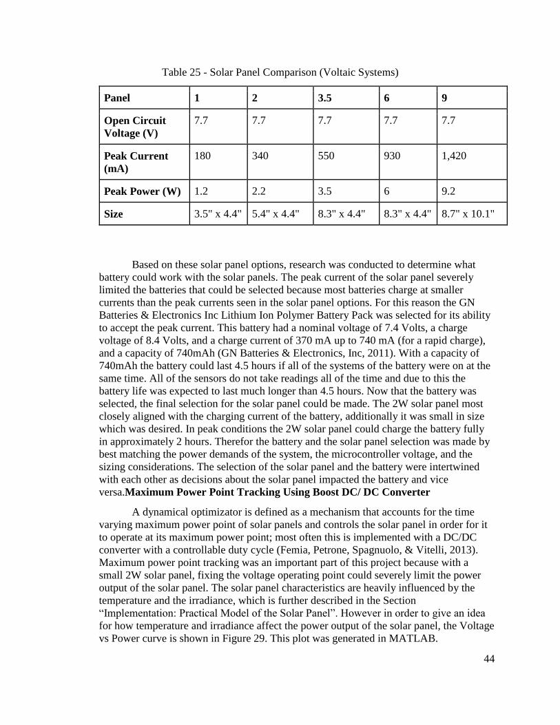
Table 25 - Solar Panel Comparison (Voltaic Systems)
Panel 1 2 3.5 6 9
Open Circuit
Voltage (V)
7.7 7.7 7.7 7.7 7.7
Peak Current
(mA)
180 340 550 930 1,420
Peak Power (W) 1.2 2.2 3.5 6 9.2
Size 3.5" x 4.4" 5.4" x 4.4" 8.3" x 4.4" 8.3" x 4.4" 8.7" x 10.1"
Based on these solar panel options, research was conducted to determine what
battery could work with the solar panels. The peak current of the solar panel severely
limited the batteries that could be selected because most batteries charge at smaller
currents than the peak currents seen in the solar panel options. For this reason the GN
Batteries & Electronics Inc Lithium Ion Polymer Battery Pack was selected for its ability
to accept the peak current. This battery had a nominal voltage of 7.4 Volts, a charge
voltage of 8.4 Volts, and a charge current of 370 mA up to 740 mA (for a rapid charge),
and a capacity of 740mAh (GN Batteries & Electronics, Inc, 2011). With a capacity of
740mAh the battery could last 4.5 hours if all of the systems of the battery were on at the
same time. All of the sensors do not take readings all of the time and due to this the
battery life was expected to last much longer than 4.5 hours. Now that the battery was
selected, the final selection for the solar panel could be made. The 2W solar panel most
closely aligned with the charging current of the battery, additionally it was small in size
which was desired. In peak conditions the 2W solar panel could charge the battery fully
in approximately 2 hours. Therefor the battery and the solar panel selection was made by
best matching the power demands of the system, the microcontroller voltage, and the
sizing considerations. The selection of the solar panel and the battery were intertwined
with each other as decisions about the solar panel impacted the battery and vice
versa.Maximum Power Point Tracking Using Boost DC/ DC Converter
A dynamical optimizator is defined as a mechanism that accounts for the time
varying maximum power point of solar panels and controls the solar panel in order for it
to operate at its maximum power point; most often this is implemented with a DC/DC
converter with a controllable duty cycle (Femia, Petrone, Spagnuolo, & Vitelli, 2013).
Maximum power point tracking was an important part of this project because with a
small 2W solar panel, fixing the voltage operating point could severely limit the power
output of the solar panel. The solar panel characteristics are heavily influenced by the
temperature and the irradiance, which is further described in the Section
“Implementation: Practical Model of the Solar Panel”. However in order to give an idea
for how temperature and irradiance affect the power output of the solar panel, the Voltage
vs Power curve is shown in Figure 29. This plot was generated in MATLAB.

45
Figure 29 - Voltage vs Power Curve for 2W Solar Panel
By inspecting the graph, it is clear that the irradiance and temperature affect the
power curve for the panel. As these conditions vary throughout the day it is important
that the solar charging system be adaptable to the varying conditions. The way a system
is able to adapt is through the dynamical optimizator, which by changing the duty cycle
changes the voltage that the solar panel operates at in order for the panel to operate at its
maximum power in any condition.
The dynamical optimizators selected for this project was a DC/DC converter with
a Boost Converter topology. This topology was used because the battery voltage would
always be higher than the solar panel voltage, therefore the voltage of the solar would
always need to be “boosted” to attain the battery voltage. A basic schematic for a
standard layout of a DC/DC boost converter is shown in the figure below, as this was
used to develop the DC/DC boost converter that was actually used with the solar panel.
First the basic schematic of a DC/DC boost converter will be described, then the way that
the values were chosen and finally how this model was adapted to do the maximum
power point tracking will be explained.
46
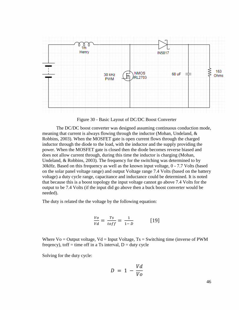
Figure 30 - Basic Layout of DC/DC Boost Converter
The DC/DC boost converter was designed assuming continuous conduction mode,
meaning that current is always flowing through the inductor (Mohan, Undeland, &
Robbins, 2003). When the MOSFET gate is open current flows through the charged
inductor through the diode to the load, with the inductor and the supply providing the
power. When the MOSFET gate is closed then the diode becomes reverse biased and
does not allow current through, during this time the inductor is charging (Mohan,
Undeland, & Robbins, 2003). The frequency for the switching was determined to by
30kHz. Based on this frequency as well as the known input voltage, 0 - 7.7 Volts (based
on the solar panel voltage range) and output Voltage range 7.4 Volts (based on the battery
voltage) a duty cycle range, capacitance and inductance could be determined. It is noted
that because this is a boost topology the input voltage cannot go above 7.4 Volts for the
output to be 7.4 Volts (if the input did go above then a buck boost converter would be
needed).
The duty is related the the voltage by the following equation:
𝑉𝑜
𝑉𝑑=
𝑇𝑠
𝑡𝑜𝑓𝑓=
1
1− 𝐷 [19]
Where Vo = Output voltage, Vd = Input Voltage, Ts = Switching time (inverse of PWM
freqency), toff = time off in a Ts interval, D = duty cycle
Solving for the duty cycle:
𝐷 = 1 − 𝑉𝑑
𝑉𝑜
47
This equation reveals that for a fixed output voltage to be attained with a variable
input voltage, when the input voltage is at a low the duty cycle is at a high and when the
input voltage is at a high the duty cycle is at a low.
Additionally the worse case capacitance could be solved for, the formula for
capacitance is:
𝐶 = 𝐼𝑜𝐷𝑇𝑠
△𝑉𝑜 [19]
Where Io = Output Current, D = Duty Cycle, Ts = Switching time, and Vo =
Voltage Ripple
To solve this equation for the largest capacitor needed, the Io was set to the
maximum output current which was the peak power input current, 340mA, the D was set
to the duty cycle at the peak power, which was 0.12, the Ts was the inverse of the 30kHz
switching frequency and the voltage ripple was 10% of the maximum voltage, 0.74 Volts.
Solving this for the capacitor size, a 1.87 uF value was found. Next the inductor value
could be extracted, in this circuit the inductor value is most important to a proper design.
The formula to find the inductor is:
L = 𝑇𝑠𝑉𝑜𝐷(1−𝐷)
2∗𝐼𝐿𝐵 [19]
Where Ts = Switching time, Vo = Output Voltage, D = Duty Cycle, ILB = Average
input current
To solve this equation for the inductor needed, again the peak parameters were
used. The switching time was the inverse of 30kHz again, the Vo was the peak power
voltage output, 6.5V, the duty cycle was the peak power duty cycle, 0.12, and the ILB was
the average current which was half of the peak power current, or 170 mA. Solving this
for the inductor size, a 67.2uH value was found.
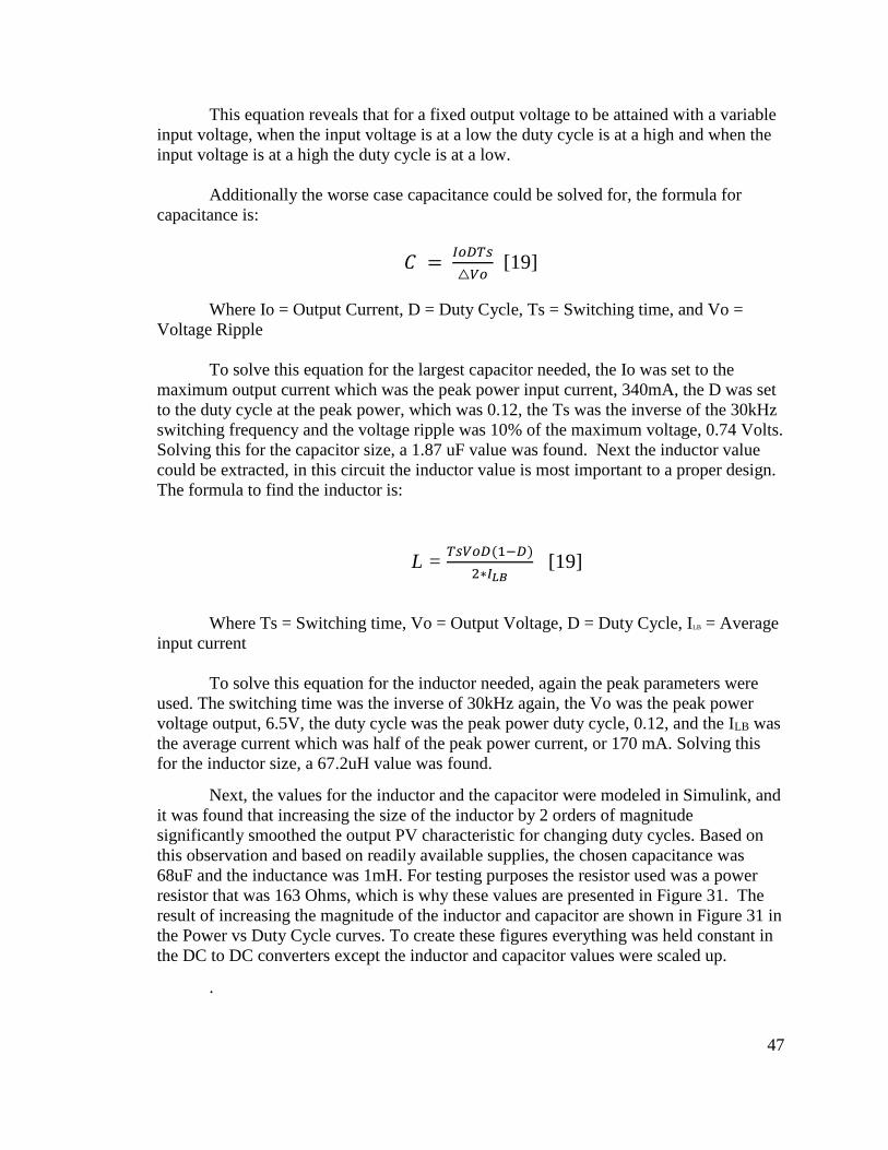
Next, the values for the inductor and the capacitor were modeled in Simulink, and
it was found that increasing the size of the inductor by 2 orders of magnitude
significantly smoothed the output PV characteristic for changing duty cycles. Based on
this observation and based on readily available supplies, the chosen capacitance was
68uF and the inductance was 1mH. For testing purposes the resistor used was a power
resistor that was 163 Ohms, which is why these values are presented in Figure 31. The
result of increasing the magnitude of the inductor and capacitor are shown in Figure 31 in
the Power vs Duty Cycle curves. To create these figures everything was held constant in
the DC to DC converters except the inductor and capacitor values were scaled up.
.
48
Original Inductor Value Increasing Inductor Value 2 Orders of
Magnitude
Figure 31 - Inductor Analysis
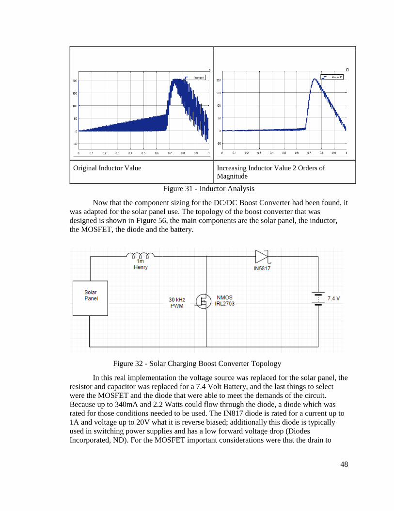
Now that the component sizing for the DC/DC Boost Converter had been found, it
was adapted for the solar panel use. The topology of the boost converter that was
designed is shown in Figure 56, the main components are the solar panel, the inductor,
the MOSFET, the diode and the battery.
Figure 32 - Solar Charging Boost Converter Topology
In this real implementation the voltage source was replaced for the solar panel, the
resistor and capacitor was replaced for a 7.4 Volt Battery, and the last things to select
were the MOSFET and the diode that were able to meet the demands of the circuit.
Because up to 340mA and 2.2 Watts could flow through the diode, a diode which was
rated for those conditions needed to be used. The IN817 diode is rated for a current up to
1A and voltage up to 20V what it is reverse biased; additionally this diode is typically
used in switching power supplies and has a low forward voltage drop (Diodes
Incorporated, ND). For the MOSFET important considerations were that the drain to

49
source voltage was small and that the gate be able to be triggered by a 3.3 Volt wave, this
was satisfied by the IRL2703 N-MOS (International Rectifier, ND).
In summary, maximum power point tracking is driven by the use of DC/DC
converters which act as dynamical optimizators because of their ability to change the
operating point of a solar panel through adjusting the duty cycle on the PWM pin. The
parts selected to be used for the DC/DC converter were the inductor, diode and the
MOSFET.
Sensing Solar Panel Voltage, Current, Power
In order to accomplish maximum power point tracking, the voltage and current of
the solar panel must to be monitored in order to interpret the power. In this way previous
values for the power of a solar panel can be compared to power values that are the result
of changing the duty cycle. This comparison will yield whether an appropriate change in
the duty cycle has been made. To monitor the voltage, current and power, the INA219
High Side Current Sensor Breakout sold by Adafruit was selected. The benefits of
choosing this specific breakout board was that it had configurable internal gain which
allowed for measurements up to a max current of 400mA with 0.1mA precision and
voltage up to 32V (Texas Instruments, 2011). This breakout board communicated with
the Arduino via I2C and included a library that could be downloaded so that simple
function calls could return the current, voltage and power.
Sensing Battery Voltage
The battery characteristic was well matched with the solar panel in that the
maximum current that the solar panel could provide would be acceptable by the battery.
However in order to monitor whether the battery was charged, in an acceptable range, or
had discharged too much the battery voltage needed to be monitored. The battery voltage
was monitored with a simple op-amp configured as a voltage follower preceded by a
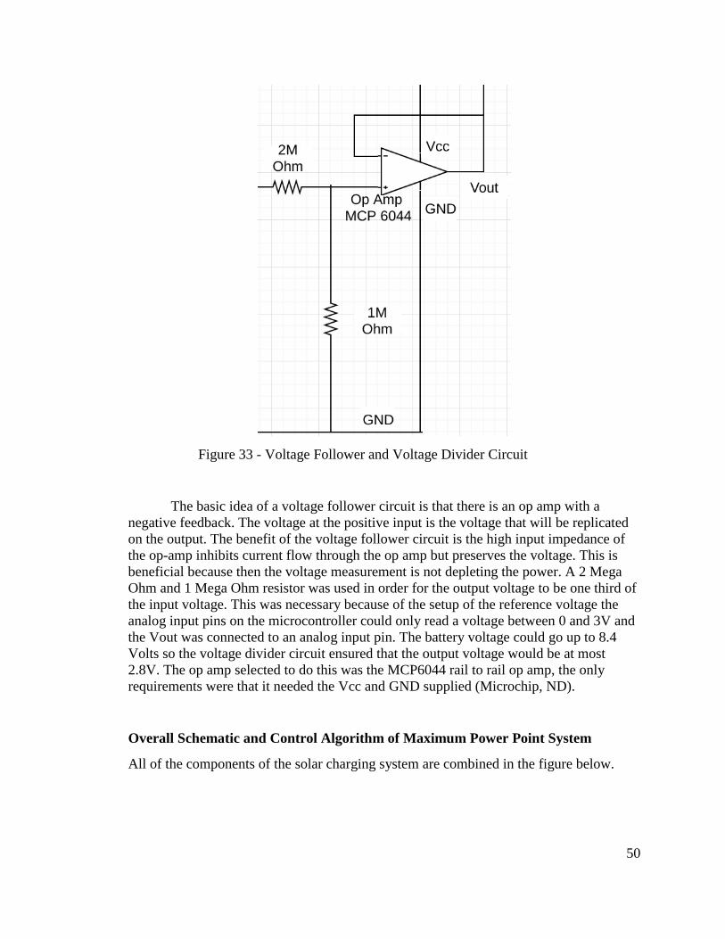
voltage divider, shown in the figure below.
50
Figure 33 - Voltage Follower and Voltage Divider Circuit
The basic idea of a voltage follower circuit is that there is an op amp with a
negative feedback. The voltage at the positive input is the voltage that will be replicated
on the output. The benefit of the voltage follower circuit is the high input impedance of
the op-amp inhibits current flow through the op amp but preserves the voltage. This is
beneficial because then the voltage measurement is not depleting the power. A 2 Mega
Ohm and 1 Mega Ohm resistor was used in order for the output voltage to be one third of
the input voltage. This was necessary because of the setup of the reference voltage the
analog input pins on the microcontroller could only read a voltage between 0 and 3V and
the Vout was connected to an analog input pin. The battery voltage could go up to 8.4
Volts so the voltage divider circuit ensured that the output voltage would be at most
2.8V. The op amp selected to do this was the MCP6044 rail to rail op amp, the only
requirements were that it needed the Vcc and GND supplied (Microchip, ND).
Overall Schematic and Control Algorithm of Maximum Power Point System
All of the components of the solar charging system are combined in the figure below.
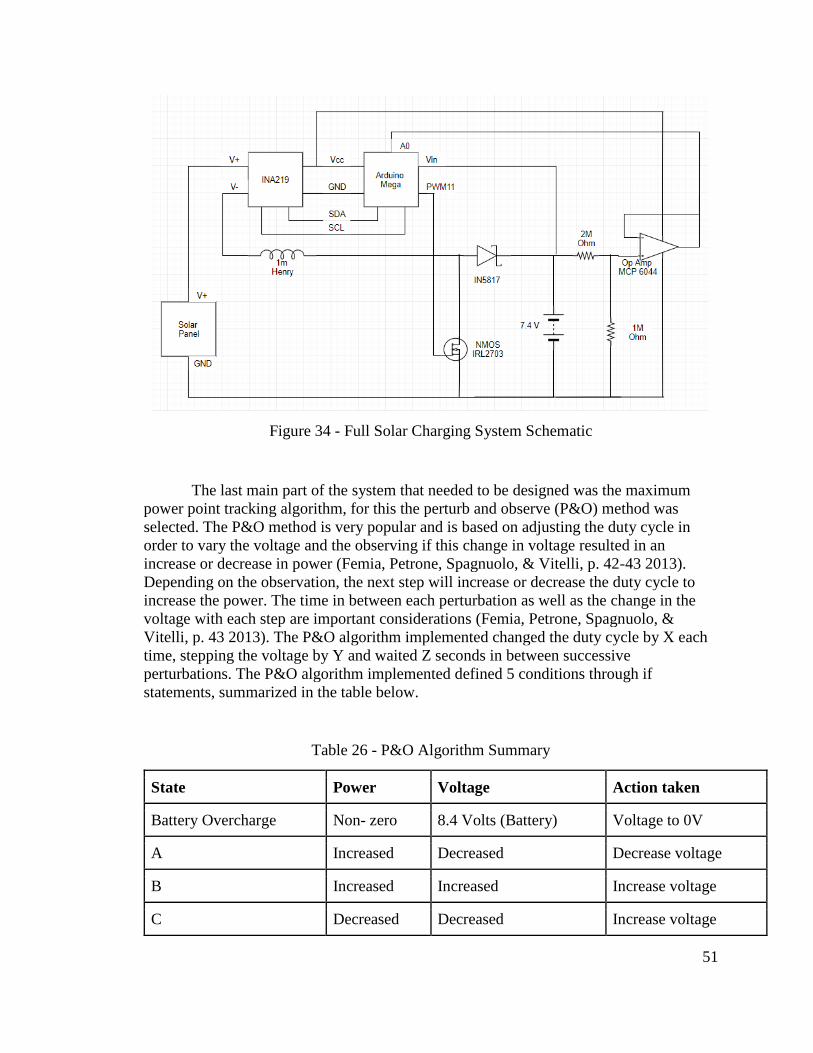
51
Figure 34 - Full Solar Charging System Schematic
The last main part of the system that needed to be designed was the maximum
power point tracking algorithm, for this the perturb and observe (P&O) method was
selected. The P&O method is very popular and is based on adjusting the duty cycle in
order to vary the voltage and the observing if this change in voltage resulted in an
increase or decrease in power (Femia, Petrone, Spagnuolo, & Vitelli, p. 42-43 2013).
Depending on the observation, the next step will increase or decrease the duty cycle to
increase the power. The time in between each perturbation as well as the change in the
voltage with each step are important considerations (Femia, Petrone, Spagnuolo, &
Vitelli, p. 43 2013). The P&O algorithm implemented changed the duty cycle by X each
time, stepping the voltage by Y and waited Z seconds in between successive
perturbations. The P&O algorithm implemented defined 5 conditions through if
statements, summarized in the table below.
Table 26 - P&O Algorithm Summary
State Power Voltage Action taken
Battery Overcharge Non- zero 8.4 Volts (Battery) Voltage to 0V
A Increased Decreased Decrease voltage
B Increased Increased Increase voltage
C Decreased Decreased Increase voltage

52
D Decreased Increased Decrease voltage
IMPLEMENTATION
Practical Model of the Solar Panel
Prior to actually implementing the 2W Voltaic Solar panel, the goal was to better
understand the behavior of it with varying temperature and irradiance conditions. This
was done by first extracting the parameters from the practical model. The practical model
of a solar panel is represented by a current source, diode, shunt resistor and a series
resistor shown in Figure 59 (Mahmoud, Xiao, & Zeineldin, 2013. The model used to find
the values for the current source, shunt resistor, and series resistor was created by
Mahmoud, Xiao, and Zeineldin and it strictly uses the data sheet values from the solar
panel. Parameterization was done using the Newton Raphson approach to find Rs and
Rsh and then the Is (short circuit current) and Ipho (photon current) could be determined..
The two equations used for the Newtown Raphson equation that resulted in finding Rs
and Rsh are shown below and the script they are used in is in Appendix I: MATLAB
Practical Model Parameter Extraction Code.
= 0
Here q is the electron charge, K is the Boltzmann constant, T is the Temperature
of the module, Ns is the number of series cells, Iph is the photon current, I s is the
saturation current, A is the ideality factor, Rs is the series resistance, Rsh is the shunt
resistor, Im is the peak power current, Vm is the peak power voltage, and Voc is the open
circuit voltage (Mahmoud, Xiao, & Zeineldin, 2013).

53
Figure 35 - Solar Panel Practical Model
Once the practical model for the solar panel was understood, the effects of the
irradiance and temperature on the solar panel could be graphed. Increasing irradiance
increases the power output of a solar panel and decreasing temperature increases the
power output of a solar panel. Mahmoud, Xiao, and Zeineldin also derived an equation
that can be used to model the effects of varying the temperature and irradiance on the PV
and IV curves using the parameters extracted from the parameterization in the previous
step, the formula is shown below.
𝐼𝑠 =𝑒
𝐵∆𝑇𝑞𝑁𝑠𝐾𝑇𝐴∗𝐺∗(𝐼𝑠𝑐+ ∝∆𝑇)
(𝐺𝐼𝑠𝑐
𝐼𝑟𝑠+1)𝑇𝑜/𝑇− 𝑒
𝐵∆𝑇𝑞𝑁𝑠𝐾𝑇𝐴
In this equation ∆𝑇 is the temperature deviation from 298K, To is the temperature at
standard temperature, which is 298K. G is the irradiance, 𝛼 is the temperature coefficient
and B is the absolute value of the voltage temperature coefficient (Mahmoud, Xiao, &
Zeineldin, 2013). This formula was applied in the MATLAB script shown in Appendix J:
MATLAB Practical Model Characteristic Curve Plotting Code in order to get the
resulting graphs shown below.
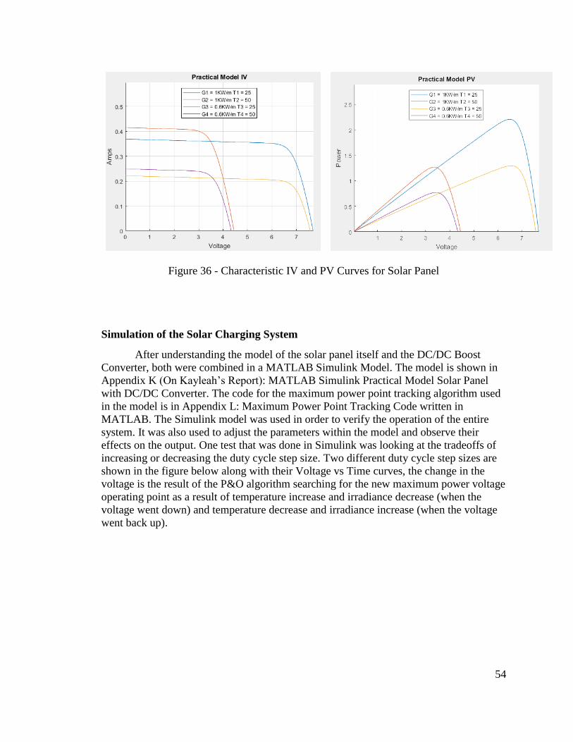
54
Figure 36 - Characteristic IV and PV Curves for Solar Panel
Simulation of the Solar Charging System
After understanding the model of the solar panel itself and the DC/DC Boost
Converter, both were combined in a MATLAB Simulink Model. The model is shown in
Appendix K (On Kayleah’s Report): MATLAB Simulink Practical Model Solar Panel
with DC/DC Converter. The code for the maximum power point tracking algorithm used
in the model is in Appendix L: Maximum Power Point Tracking Code written in
MATLAB. The Simulink model was used in order to verify the operation of the entire
system. It was also used to adjust the parameters within the model and observe their
effects on the output. One test that was done in Simulink was looking at the tradeoffs of
increasing or decreasing the duty cycle step size. Two different duty cycle step sizes are
shown in the figure below along with their Voltage vs Time curves, the change in the
voltage is the result of the P&O algorithm searching for the new maximum power voltage
operating point as a result of temperature increase and irradiance decrease (when the
voltage went down) and temperature decrease and irradiance increase (when the voltage
went back up).

55
Duty Cycle Step 0.05 Duty Cycle Step 0.01
Figure 37 –Duty Cycle Simulations
The notable observation from these graphs is that there is a tradeoff between the
speed it takes to reach the maximum power and the oscillations around the maximum
power once the voltage reaches the maximum power. When the duty cycle step size is
large, maximum power is more rapidly found but there are larger oscillations around the
maximum power point, causing loss of power. Methods do exist to vary the size of the
duty cycle step based on proximity to the maximum power point, however these were not
implemented.
Experimental Results from the Solar Charging System
The entire constructed system is shown in the figure below, the urban pollution
mapping, the DC/DC converter, the battery, and the solar panel are highlighted.
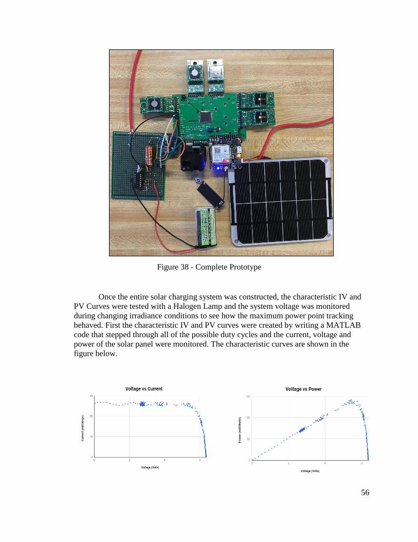
56
Figure 38 - Complete Prototype
Once the entire solar charging system was constructed, the characteristic IV and
PV Curves were tested with a Halogen Lamp and the system voltage was monitored
during changing irradiance conditions to see how the maximum power point tracking
behaved. First the characteristic IV and PV curves were created by writing a MATLAB
code that stepped through all of the possible duty cycles and the current, voltage and
power of the solar panel were monitored. The characteristic curves are shown in the
figure below.
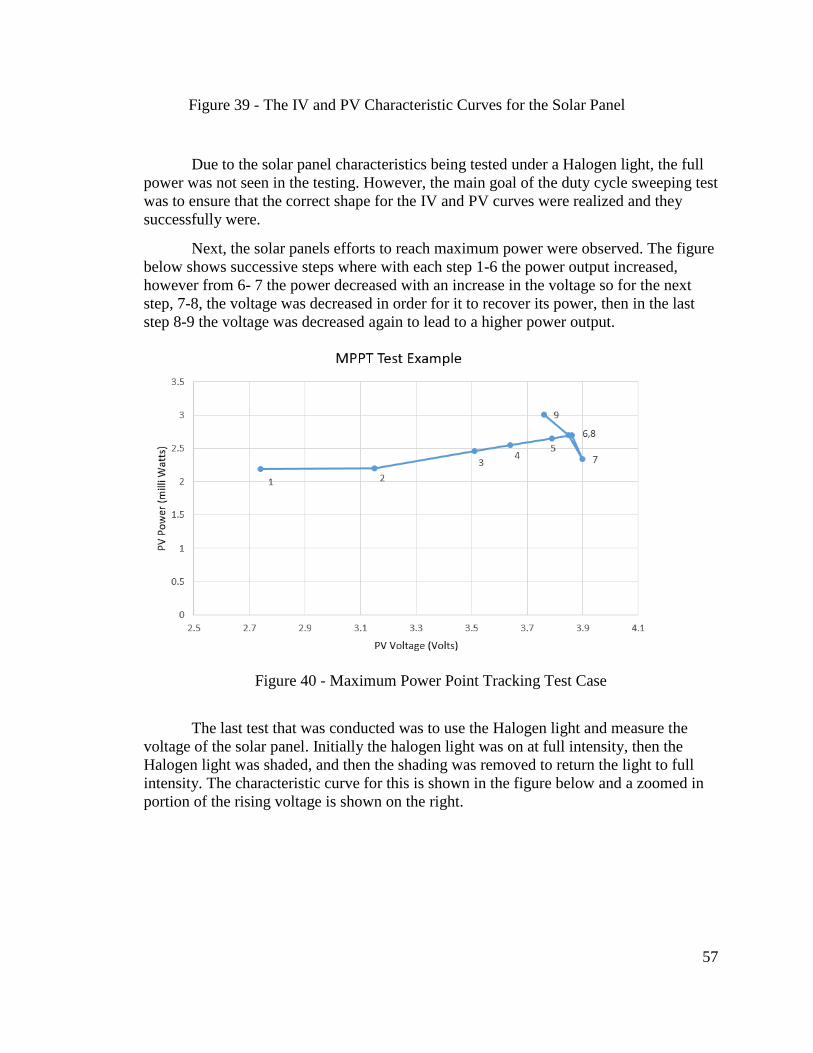
57
Figure 39 - The IV and PV Characteristic Curves for the Solar Panel
Due to the solar panel characteristics being tested under a Halogen light, the full
power was not seen in the testing. However, the main goal of the duty cycle sweeping test
was to ensure that the correct shape for the IV and PV curves were realized and they
successfully were.
Next, the solar panels efforts to reach maximum power were observed. The figure
below shows successive steps where with each step 1-6 the power output increased,
however from 6- 7 the power decreased with an increase in the voltage so for the next
step, 7-8, the voltage was decreased in order for it to recover its power, then in the last
step 8-9 the voltage was decreased again to lead to a higher power output.
Figure 40 - Maximum Power Point Tracking Test Case
The last test that was conducted was to use the Halogen light and measure the
voltage of the solar panel. Initially the halogen light was on at full intensity, then the
Halogen light was shaded, and then the shading was removed to return the light to full
intensity. The characteristic curve for this is shown in the figure below and a zoomed in
portion of the rising voltage is shown on the right.
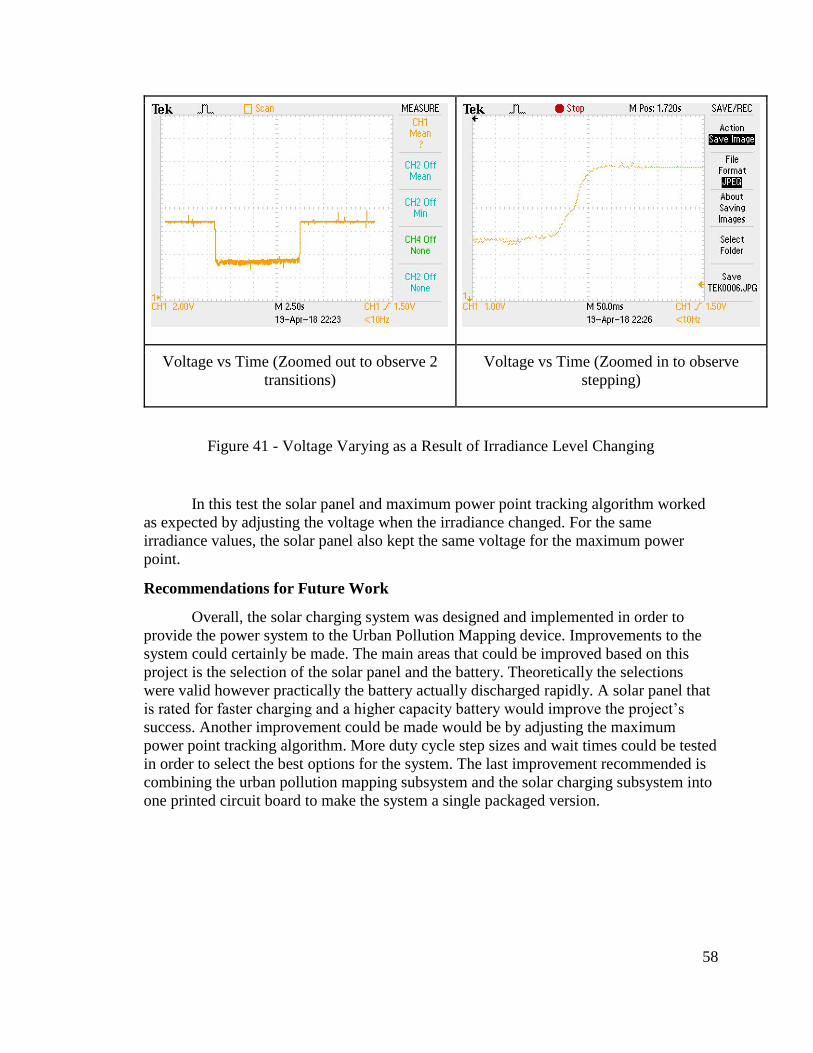
58
Voltage vs Time (Zoomed out to observe 2
transitions)
Voltage vs Time (Zoomed in to observe
stepping)
Figure 41 - Voltage Varying as a Result of Irradiance Level Changing
In this test the solar panel and maximum power point tracking algorithm worked
as expected by adjusting the voltage when the irradiance changed. For the same
irradiance values, the solar panel also kept the same voltage for the maximum power
point.
Recommendations for Future Work
Overall, the solar charging system was designed and implemented in order to
provide the power system to the Urban Pollution Mapping device. Improvements to the
system could certainly be made. The main areas that could be improved based on this
project is the selection of the solar panel and the battery. Theoretically the selections
were valid however practically the battery actually discharged rapidly. A solar panel that
is rated for faster charging and a higher capacity battery would improve the project’s
success. Another improvement could be made would be by adjusting the maximum
power point tracking algorithm. More duty cycle step sizes and wait times could be tested
in order to select the best options for the system. The last improvement recommended is
combining the urban pollution mapping subsystem and the solar charging subsystem into
one printed circuit board to make the system a single packaged version.
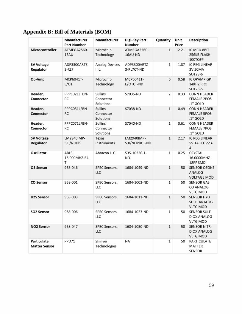
59
Appendix B: Bill of Materials (BOM)
Manufacturer Part Number
Manufacturer Digi-Key Part Number
Quantity Unit Price
Description
Microcontroller ATMEGA2560-16AU
Microchip Technology
ATMEGA2560-16AU-ND
1 12.21 IC MCU 8BIT 256KB FLASH 100TQFP
3V Voltage Regulator
ADP3300ARTZ-3-RL7
Analog Devices Inc.
ADP3300ARTZ-3-RL7CT-ND
1 1.87 IC REG LINEAR 3V 50MA SOT23-6
Op-Amp MCP6041T-E/OT
Microchip Technology
MCP6041T-E/OTCT-ND
6 0.58 IC OPAMP GP 14KHZ RRO SOT23-5
Header, Connector
PPPC021LFBN-RC
Sullins Connector Solutions
S7035-ND 2 0.33 CONN HEADER FEMALE 2POS .1" GOLD
Header, Connector
PPPC051LFBN-RC
Sullins Connector Solutions
S7038-ND 1 0.49 CONN HEADER FEMALE 5POS .1" GOLD
Header, Connector
PPPC071LFBN-RC
Sullins Connector Solutions
S7040-ND 1 0.61 CONN HEADER FEMALE 7POS .1" GOLD
5V Voltage Regulator
LM2940IMP-5.0/NOPB
Texas Instruments
LM2940IMP-5.0/NOPBCT-ND
1 2.17 IC REG LINEAR 5V 1A SOT223-4
Oscillator ABLS-16.000MHZ-B4-T
Abracon LLC 535-10226-1-ND
1 0.25 CRYSTAL 16.0000MHZ 18PF SMD
O3 Sensor 968-046 SPEC Sensors, LLC
1684-1049-ND 1 50 SENSOR OZONE ANALOG VOLTAGE MOD
CO Sensor 968-001 SPEC Sensors, LLC
1684-1002-ND 1 50 SENSOR GAS CO ANALOG VLTG MOD
H2S Sensor 968-003 SPEC Sensors, LLC
1684-1011-ND 1 50 SENSOR HYD SULF ANALOG VLTG MOD
SO2 Sensor 968-006 SPEC Sensors, LLC
1684-1023-ND 1 50 SENSOR SULF DIOX ANALOG VLTG MOD
NO2 Sensor 968-047 SPEC Sensors, LLC
1684-1050-ND 1 50 SENSOR NITR DIOX ANALOG VLTG MOD
Particulate Matter Sensor
PPD71 Shinyei Technologies
NA 1 50 PARTICULATE MATTER SENSOR
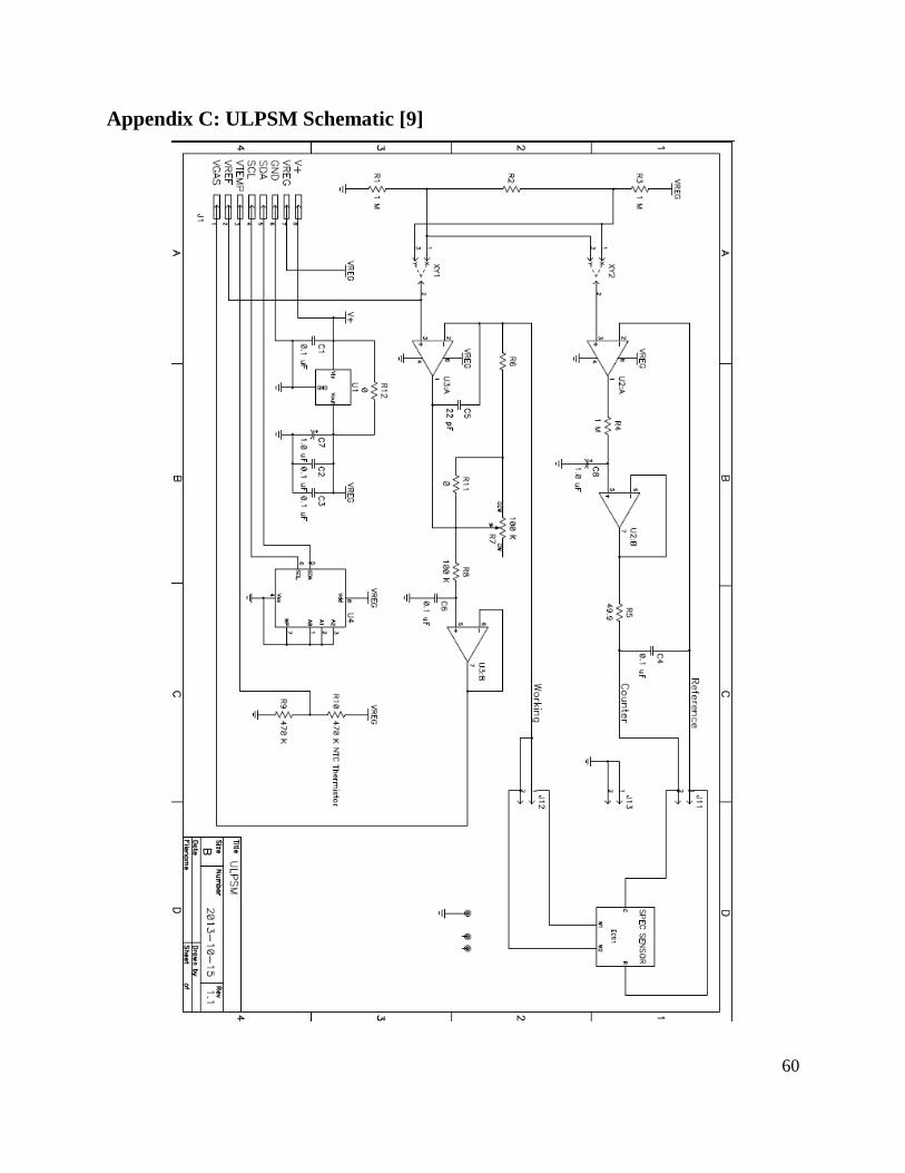
60
Appendix C: ULPSM Schematic [9]
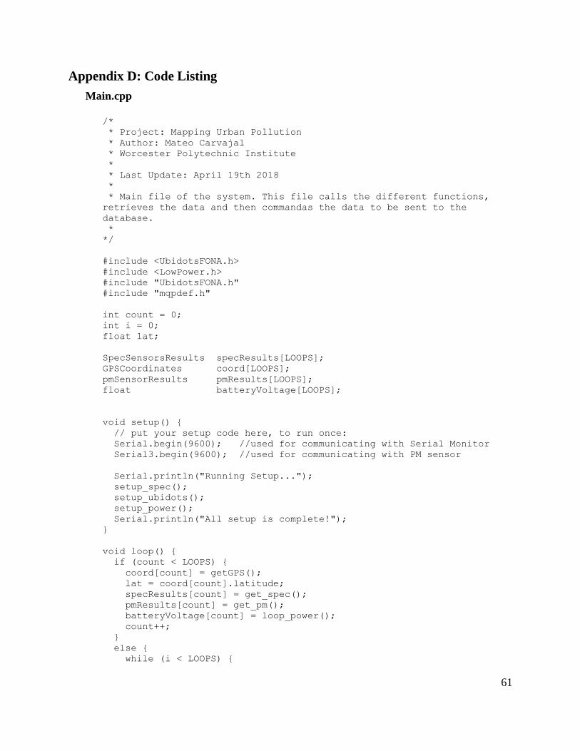
61
Appendix D: Code Listing
Main.cpp
/*
* Project: Mapping Urban Pollution
* Author: Mateo Carvajal
* Worcester Polytechnic Institute
*
* Last Update: April 19th 2018
*
* Main file of the system. This file calls the different functions,
retrieves the data and then commandas the data to be sent to the
database.
*
*/
#include <UbidotsFONA.h>
#include <LowPower.h>
#include "UbidotsFONA.h"
#include "mqpdef.h"
int count = 0;
int i = 0;
float lat;
SpecSensorsResults specResults[LOOPS];
GPSCoordinates coord[LOOPS];
pmSensorResults pmResults[LOOPS];
float batteryVoltage[LOOPS];
void setup() {
// put your setup code here, to run once:
Serial.begin(9600); //used for communicating with Serial Monitor
Serial3.begin(9600); //used for communicating with PM sensor
Serial.println("Running Setup...");
setup_spec();
setup_ubidots();
setup_power();
Serial.println("All setup is complete!");
}
void loop() {
if (count < LOOPS) {
coord[count] = getGPS();
lat = coord[count].latitude;
specResults[count] = get_spec();
pmResults[count] = get_pm();
batteryVoltage[count] = loop_power();
count++;
}
else {
while (i < LOOPS) {

62
send2Ubidots(specResults[i], coord[i], pmResults[i],
batteryVoltage[i]);
i++;
}
count = 0;
i = 0;
}
delay(1000);
}
Mqpdef.h
/*
* Project: Mapping Urban Pollution
* Author: Mateo Carvajal
* Worcester Polytechnic Institute
*
* Last Update: April 19th 2018
*
* This header file defines a number of data structure and assigns
values to constants.
*/
#ifndef mqpdef_h
#define mqpdef_h
#include "Arduino.h"
//#include "Adafruit_FONA.h"
//#include <SoftwareSerial.h>
/*
* General
* ADCRESOLUTION = 1.1/2^10 = 1.1/1024 = 0.00107421875
* ADCRESOLUTION = 3/2^10 = 3/1024 = 0.00322265625
* DEBUG
*/
#define DEBUG false //When true Debug Information is printed to the
serial port.
#define ADC_RESOLUTION 0.00292968 // ADC_RESOLUTION = 3V / 1024
#define LOOPS 5
/* SPEC Sensor
* CO
* NO2
* SO2
* H2S
* O3
*
* VREF
* VGAS
*/ //TABLE BELOW | Arduino Mega
| AtMega2560 Direct
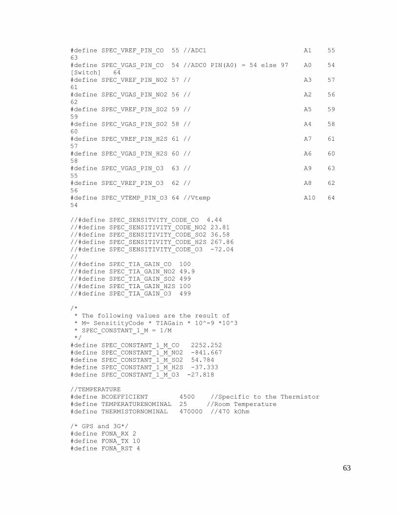
63
#define SPEC_VREF_PIN_CO 55 //ADC1 A1 55
63
#define SPEC_VGAS_PIN_CO 54 //ADC0 PIN(A0) = 54 else 97 A0 54
[Switch] 64
#define SPEC_VREF_PIN_NO2 57 // A3 57
61
#define SPEC_VGAS_PIN_NO2 56 // A2 56
62
#define SPEC_VREF_PIN_SO2 59 // A5 59
59
#define SPEC_VGAS_PIN_SO2 58 // A4 58
60
#define SPEC_VREF_PIN_H2S 61 // A7 61
57
#define SPEC_VGAS_PIN_H2S 60 // A6 60
58
#define SPEC_VGAS_PIN_O3 63 // A9 63
55
#define SPEC_VREF_PIN_O3 62 // A8 62
56
#define SPEC_VTEMP_PIN_O3 64 //Vtemp A10 64
54
//#define SPEC_SENSITVITY_CODE_CO 4.44
//#define SPEC_SENSITIVITY_CODE_NO2 23.81
//#define SPEC_SENSITIVITY_CODE_SO2 36.58
//#define SPEC_SENSITIVITY_CODE_H2S 267.86
//#define SPEC_SENSITIVITY_CODE_O3 -72.04
//
//#define SPEC_TIA_GAIN_CO 100
//#define SPEC_TIA_GAIN_NO2 49.9
//#define SPEC_TIA_GAIN_SO2 499
//#define SPEC_TIA_GAIN_H2S 100
//#define SPEC_TIA_GAIN_O3 499
/*
* The following values are the result of
* M= SensitityCode * TIAGain * 10^-9 *10^3
* SPEC_CONSTANT_1_M = 1/M
*/
#define SPEC_CONSTANT_1_M_CO 2252.252
#define SPEC_CONSTANT_1_M_NO2 -841.667
#define SPEC_CONSTANT_1_M_SO2 54.784
#define SPEC_CONSTANT_1_M_H2S -37.333
#define SPEC_CONSTANT_1_M_O3 -27.818
//TEMPERATURE
#define BCOEFFICIENT 4500 //Specific to the Thermistor
#define TEMPERATURENOMINAL 25 //Room Temperature
#define THERMISTORNOMINAL 470000 //470 kOhm
/* GPS and 3G*/
#define FONA_RX 2
#define FONA_TX 10
#define FONA_RST 4
64
//SoftwareSerial fonaSS = SoftwareSerial(FONA_TX, FONA_RX);
//SoftwareSerial *fonaSerial = &fonaSS;
/* PM Sensor */
typedef struct pmSensorResults{
uint8_t stx;
uint8_t d1;
uint8_t d2;
uint8_t d3;
uint16_t d4;
uint16_t d5;
uint16_t d6;
uint16_t d7;
uint16_t d8;
uint16_t d9;
uint16_t d10;
uint16_t d11;
uint16_t d12;
uint32_t d13;
uint8_t etx;
uint8_t d14;
uint8_t eot;
float pm05_occupancy;
float pm07_occupancy;
float pm10_occupancy;
float pm25_occupancy;
} ;//Measurements
//Spec functions
typedef struct SpecSensorsResults{
float CO;
float NO2;
float SO2;
float H2S;
float O3;
float TEMP;
};
void setup_spec();
SpecSensorsResults get_spec();
void specDebug(SpecSensorsResults specResults);
//GPS & 3G Functions
#define FONA_RX 2
#define FONA_TX 10
#define FONA_RST 4
//typedef struct GPSCoordinates{
// float latitude;
// float longitude;
// float speed_kph;
// float heading;
// float altitude;
//};
65
//void setup_gps();
//GPSCoordinates get_gps();
pmSensorResults get_pm();
//Ubidots
void setup_ubidots();
GPSCoordinates getGPS();
void send2Ubidots(SpecSensorsResults specResults, GPSCoordinates coord,
pmSensorResults pmResults, float batteryVoltage );
//Power
void setup_power();
float loop_power();
void test_power (void) ;
#endif
SpecSensorCode.cpp
/*
* Project: Mapping Urban Pollution
* Author: Mateo Carvajal
* Worcester Polytechnic Institute
*
* The following code was written to read and calculate the
concentration of five air pollutatnts:
* 1. Carbon Monoxide
* 2. Nitrogen Dioxide
* 3. Sulpur Dioxide
* 4. Hydrogen Sulphide
* 5. Ozone
*
* The constants used in this file are declared in the 'mqpdef.h'
file.
*
* The function returns a pointer to a struct that holds the
concentration result for each air pollutant.
*/
#include "mqpdef.h"
float vref_co = 0;
float vgas_co = 0;
float vref_no2 = 0;
float vgas_no2 = 0;
float vref_so2 = 0;
float vgas_so2 = 0;
float vref_h2s = 0;
float vgas_h2s = 0;
float vref_o3 = 0;
float vgas_o3 = 0;
float temp_o3 = 0;
float tempVin = 0;
float concentration_co = 0;
66
float concentration_no2 = 0;
float concentration_so2 = 0;
float concentration_h2s = 0;
float concentration_o3 = 0;
float concentration_co_past = 0;
float concentration_no2_past = 0;
float concentration_so2_past = 0;
float concentration_h2s_past = 0;
float concentration_o3_past = 0;
void setup_spec(){
Serial.println("Spec Setup...");
analogReference(EXTERNAL); //Connected to the 3V Rail
pinMode(SPEC_VREF_PIN_CO,INPUT);
pinMode(SPEC_VGAS_PIN_CO,INPUT);
pinMode(SPEC_VREF_PIN_NO2,INPUT);
pinMode(SPEC_VGAS_PIN_NO2,INPUT);
pinMode(SPEC_VREF_PIN_SO2,INPUT);
pinMode(SPEC_VGAS_PIN_SO2,INPUT);
pinMode(SPEC_VREF_PIN_H2S,INPUT);
pinMode(SPEC_VGAS_PIN_H2S,INPUT);
pinMode(SPEC_VTEMP_PIN_O3,INPUT);
pinMode(SPEC_VREF_PIN_O3,INPUT);
pinMode(SPEC_VGAS_PIN_O3,INPUT);
Serial.println("SPEC SENSORS SETUP COMPLETE");
}
SpecSensorsResults get_spec(){
SpecSensorsResults specResults;
//Carbon Monoxide
vref_co = analogRead(SPEC_VREF_PIN_CO) *ADC_RESOLUTION; // read
the input pin
vgas_co = analogRead(SPEC_VGAS_PIN_CO) *ADC_RESOLUTION;
concentration_co = (vgas_co - vref_co) * SPEC_CONSTANT_1_M_CO;
//Nitrogen Dioxide
vref_no2 = analogRead(SPEC_VREF_PIN_NO2) * ADC_RESOLUTION; //
read the input pin
vgas_no2 = analogRead(SPEC_VGAS_PIN_NO2) * ADC_RESOLUTION;
concentration_no2 = (vgas_no2 - vref_no2)*SPEC_CONSTANT_1_M_NO2;
//Sulphur Dioxide
vref_so2 = analogRead(SPEC_VREF_PIN_SO2) * ADC_RESOLUTION; //
read the input pin
vgas_so2 = analogRead(SPEC_VGAS_PIN_SO2) * ADC_RESOLUTION;
concentration_so2 = (vgas_so2 - vref_so2)*SPEC_CONSTANT_1_M_SO2;
//Hydrogen Sulphide
vref_h2s = analogRead(SPEC_VREF_PIN_H2S) * ADC_RESOLUTION; //
read the input pin
vgas_h2s = analogRead(SPEC_VGAS_PIN_H2S) * ADC_RESOLUTION;
concentration_h2s = (vgas_h2s - vref_h2s)*SPEC_CONSTANT_1_M_H2S;
67
//Ozone
vref_o3 = analogRead(SPEC_VREF_PIN_O3) * ADC_RESOLUTION; // read
the input pin
vgas_o3 = analogRead(SPEC_VGAS_PIN_O3) * ADC_RESOLUTION;
concentration_o3 = (vgas_o3 - vref_o3)*SPEC_CONSTANT_1_M_O3;
//Temperature
tempVin = analogRead(SPEC_VTEMP_PIN_O3) * ADC_RESOLUTION;
temp_o3 = (3 / tempVin) -1 ;
temp_o3 = log(temp_o3);
temp_o3 /= BCOEFFICIENT;
temp_o3 += 1.0 / (TEMPERATURENOMINAL + 273.15);
temp_o3 = 1.0 / temp_o3;
temp_o3 -= 273.15;
if(concentration_co >= 0){
specResults.CO = concentration_co;
concentration_co_past = concentration_co;
}
else{
specResults.CO = concentration_co_past;
}
if(concentration_no2 >= 0.0){
specResults.NO2 = concentration_no2;
concentration_no2_past = concentration_no2;
}
else{
specResults.NO2 = concentration_no2_past;
}
if(concentration_so2 >= 0.0){
specResults.SO2 = concentration_so2;
concentration_so2_past = concentration_so2;
}
else{
specResults.SO2 = concentration_so2_past;
}
if(concentration_h2s >= 0.0){
specResults.H2S = concentration_h2s;
concentration_h2s_past = concentration_h2s;
}
else{
specResults.H2S = concentration_h2s_past;
}
if(concentration_o3 >= 0.0){
specResults.O3 = concentration_o3;
concentration_o3_past = concentration_o3;
}
else{
specResults.O3 = concentration_o3_past;
}
specResults.TEMP = temp_o3;
if(DEBUG){
68
specDebug(specResults);
}
return specResults;
}
void specDebug(SpecSensorsResults specResults){
// delay(1000);
Serial.println("_________________");
Serial.print("Carbon Monoxide Concentration: "); //
debug value
Serial.print(specResults.CO,15);
Serial.print(" ppm\n");
Serial.print("Nitrogen Dioxide Concentration: "); //
debug value
Serial.print(specResults.NO2,15);
Serial.print(" ppm\n");
Serial.print("Sulphur Dioxide Concentration: "); //
debug value
Serial.print(specResults.SO2,15);
Serial.print(" ppm\n");
Serial.print("Hydrogen Sulphide Concentration: "); //
debug value
Serial.print(specResults.H2S,15);
Serial.print(" ppm\n");
Serial.print("Ozone Concentration: "); //
debug value
Serial.print(specResults.O3,15);
Serial.print(" ppm\n");
}
pmSensorCode.cpp
/*
* Project: Mapping Urban Pollution
* Author: Mateo Carvajal
* Worcester Polytechnic Institute
*
* Last Update: Feb 6th 2018
*
* The following code works with a Shinyei PPD 71 Sensor. This sensor
is designed to measure particulate matter.
* The following code only needs to have connected pins 1,3 and 4. Pin
2 is left open(not grounded).
*
* Pins
* 1 -> GND
* 2 -> Output Mode(Open- Automatic Transmission, Grounded- Command
Response Mode
* 3 -> PWR 5V
69
* 4 -> TX (Output 3.3V)
* 5 -> RX (Input 3.3V)
* ________
* | | Bottom View
* | PM |
* | SENSOR |
* |__|_____|
* 12345 pins
*/
#include "mqpdef.h"
//Buffer to store information from the sensor
char Buffer[29];
//pmSensorDataStructure pmLog[100];
//
//void setup() {
// //Setup Serial3 to communicate with Shinyei
// Serial.begin(9600);
// Serial3.begin(9600);
//}
/*
* pmSesorResults get_pm()
* returns the values obtained from the PMSensor as the occupancy
ratio.
*/
pmSensorResults get_pm(){
pmSensorResults pmReading;
//Data is received in bytes. It is put into the buffer array.
if(Serial3.available()){
Serial3.readBytesUntil('0x04', Buffer, 29);
}
//D3, D11 and D14 are represented in two bytes. Hence we take the
first byte,
//shift it left by a byte and then OR it with the second byte.
uint16_t d3 = (uint16_t)Buffer[3] << 8;
d3 |= Buffer[4];
// uint16_t d3 = d3_bigEndian ;//SwapBits(d3_bigEndian);
// SwapBits(65281);
uint16_t d4 = (uint16_t)Buffer[5] << 8;
d4 |= Buffer[6];
uint16_t d5 = (uint16_t)Buffer[7] << 8;
d5 |= Buffer[8];
uint16_t d6 = (uint16_t)Buffer[9] << 8;
d6 |= Buffer[10];
uint16_t d7 = (uint16_t)Buffer[11] << 8;
d7 |= Buffer[12];
70
uint16_t d8 = (uint16_t)Buffer[13] << 8;
d8 |= Buffer[14];
uint16_t d9 = (uint16_t)Buffer[15] << 8;
d9 |= Buffer[16];
uint16_t d10 = (uint16_t)Buffer[17] << 8;
d10 |= Buffer[18];
uint16_t d11 = (uint16_t)Buffer[19] << 8;
d11 |= Buffer[20];
//D13 is 4 bytes long
uint32_t d13 = (uint32_t)Buffer[22]<<8; //First 16
d13 |= Buffer[23];
d13 << 8; //Second 24
d13 |= Buffer[24];
d13 << 8; //Third 32
d13 |= Buffer[25];
//Assignment of values to fields in the pmReading
pmReading.stx = (uint8_t)Buffer[0];
pmReading.d1 = (uint8_t)Buffer[1];
pmReading.d2 = (uint8_t)Buffer[2];
pmReading.d3 = d3;
pmReading.d4 = d4;
pmReading.d5 = d5;
pmReading.d6 = d6;
pmReading.d7 = d7;
pmReading.d8 = d8;
pmReading.d9 = d9;
pmReading.d10= d10;
pmReading.d11= d11;
pmReading.d12= (uint8_t)Buffer[21];
pmReading.d13= d13;
pmReading.etx= (uint8_t)Buffer[26];
pmReading.d14= (uint8_t)Buffer[27];
pmReading.eot= (uint8_t)Buffer[28];
pmReading.pm05_occupancy = d7/10000;
pmReading.pm07_occupancy = d8/10000;
pmReading.pm10_occupancy = d9/10000;
pmReading.pm25_occupancy = d10/10000;
if(DEBUG){
printValues(pmReading);
}
return pmReading;
}
/*
* printValues()
* @param pmSensorDataStructure pmData
71
* @return void
*
* The following function is called if DEBUG is true. It will print out
all the values received to the buffer.
*/
void printValues(pmSensorResults pmData){
Serial.println("______________________________");
Serial.println("Debugging");
Serial.print("D1 Number of Bytes Transmitted:");
Serial.println(pmData.d1);
Serial.print("D2 Command(Fixed Value): ");
Serial.println(pmData.d2);
Serial.print("D3 Mass Concentration 10s: ");
Serial.println(pmData.d3);
Serial.print("D4 Mass Concentration 30s: ");
Serial.println(pmData.d4);
Serial.print("D5 Mass Concentration 60s: ");
Serial.println(pmData.d5);
Serial.print("D6 Mass Concentration 180s: ");
Serial.println(pmData.d6);
Serial.print("D7 0.5um Pulse Ratio Output: ");
Serial.println(pmData.d7);
Serial.print("D8 0.7um Pulse Ratio Output: ");
Serial.println(pmData.d8);
Serial.print("D9 1.0um Pulse Ratio Output: ");
Serial.println(pmData.d9);
Serial.print("D10 2.5um Pulse Ratio Output: ");
Serial.println(pmData.d10);
Serial.print("D11 Status: ");
Serial.println(pmData.d11);
Serial.print("D12 Software Version: ");
Serial.println(pmData.d12);
Serial.print("D13 Production Number: ");
Serial.println(pmData.d13);
Serial.print("ETX: ");
Serial.println(pmData.etx);
Serial.print("D14 Checksum: ");
Serial.println(pmData.d14);
Serial.print("EOT: ");
Serial.println(pmData.eot);
Serial.print("PM 0.5 Occupancy: ");
Serial.println(pmData.pm05_occupancy);
Serial.print("PM 2.5 Occupancy: ");
Serial.println(pmData.pm25_occupancy);
}
Power.cpp
/*
* Project: Mapping Urban Pollution
* Author: Kayleah Griffen
* Worcester Polytechnic Institute
*
72
* Last Update: April 19th 2018
*
* The following codes takes care of monitoring the power of
* the solar panel and charging the battery. It charges the battery
using
* maximum power point tracking(MPPT)
*
*/
#include <Wire.h>
#include <Adafruit_INA219.h>
#include "mqpdef.h"
Adafruit_INA219 ina219_PV;
//Adafruit_INA219 ina219_Battery(0x41);
int pin = 11;
//float current_mA;
float Power;
float Old_Power;
int Duty_Cycle;
int Dstep;
int Duty_Cycle_Cutoff;
float Voltage;
float Old_Voltage;
float current_mA;
float Old_Current;
float Battery_Voltage;
//float Battery_Current = 0;
//int Max_Battery_Current = 370;
float Max_Battery_Voltage = 8.4;
float Other_power;
int sensorValue;
float voltage;
void setup_power(void){
Duty_Cycle = 40;
Dstep = 1 ;
Duty_Cycle_Cutoff = 0;
Old_Voltage = 0;
current_mA = 0;
Battery_Voltage = 0;
73
Max_Battery_Voltage = 8.4;
int myEraser = 7; // this is 111 in binary and is
used as an eraser
TCCR1B &= ~myEraser; // this operation (AND plus NOT), set the
three bits in TCCR1B to 0
int myPrescaler = 1; // this could be a number in [1 , 6].
In this case, 3 corresponds in binary to 011.
TCCR1B |= myPrescaler; //this operation (OR), replaces the last
three bits in TCCR2B with our new value 011
Serial.begin(9600);
analogReference(EXTERNAL);
Serial.println("Hello!");
// Initialize the INA219.
// By default the initialization will use the largest range (32V,
2A). However
// you can call a setCalibration function to change this range (see
comments).
ina219_PV.begin();
//ina219_Battery.begin();
// To use a slightly lower 32V, 1A range (higher precision on amps):
//ina219.setCalibration_32V_1A();
// Or to use a lower 16V, 400mA range (higher precision on volts and
amps):
ina219_PV.setCalibration_16V_400mA();
//ina219_Battery.setCalibration_16V_400mA();
Serial.println("Setup complete");
}
float loop_power(){
analogWrite(pin, Duty_Cycle) ;
Old_Power = Old_Voltage * Old_Current;
Voltage = ina219_PV.getBusVoltage_V();
current_mA = ina219_PV.getCurrent_mA();
Power = Voltage * current_mA;
Other_power = ina219_PV.getPower_mW();
sensorValue = analogRead(A11);
// Convert the analog reading (which goes from 0 - 1023) to a voltage
(0 - 5V):
voltage = sensorValue * (3.0 / 1023.0) * 3;
// print out the value you read:
Serial.print("Duty Cycle: "); Serial.print(Duty_Cycle);
Serial.println("/256");
Serial.print("PV Voltage: "); Serial.print(Voltage);
Serial.println(" V");
Serial.print("PV Current: "); Serial.print(current_mA);
Serial.println(" mA");
Serial.print("PV Power: "); Serial.print(Power);
Serial.println(" mW");
74
Serial.print("Old Voltage: "); Serial.print(Old_Voltage);
Serial.println(" V");
Serial.print("Old Power: "); Serial.print(Old_Power);
Serial.println(" mW");
Serial.print("Battery Voltage: "); Serial.print(voltage);
Serial.println(" V");
if (Duty_Cycle < 0){
Duty_Cycle = 10; //resetting up a little higher to prevent negative
}
if ((Power > Old_Power) and (Voltage > Old_Voltage)) {
Duty_Cycle = Duty_Cycle - Dstep;
Serial.println("A");
}
//Increasing power, Decreasing Voltage
//keep decreasing volgate by increasing duty cycle
else if ((Power >= Old_Power) and (Voltage <= Old_Voltage)) {
Duty_Cycle = Duty_Cycle + Dstep;
Serial.println("B");
}
//Decreasing power, Increasing Voltage
//instead decrease volgate by increasing duty cycle
else if ((Power < Old_Power) and (Voltage >= Old_Voltage)) {
Duty_Cycle = Duty_Cycle + Dstep;
Serial.println("C");
}
//Decreasing power, Decreasing Voltage
//instead increase volgate by decreasing duty cycle
else if ((Power < Old_Power) and (Voltage <= Old_Voltage)) {
Duty_Cycle = Duty_Cycle - Dstep;
Serial.println("D");
}
analogWrite(pin, Duty_Cycle) ;// use pins 12 or 11
Serial.println("");
//set the olds
Old_Power = Power;
Old_Voltage = Voltage;
Old_Current = current_mA;
return Voltage;
}
void test_power (void) {
Duty_Cycle = 0;
int max_duty_cycle = 256;
while (max_duty_cycle > Duty_Cycle){
analogWrite(pin, Duty_Cycle) ;
75
Voltage = ina219_PV.getBusVoltage_V();
current_mA = ina219_PV.getCurrent_mA();
Power = Voltage * current_mA;
Other_power = ina219_PV.getPower_mW();
Serial.print("Duty Cycle: "); Serial.print(Duty_Cycle);
Serial.println("/256");
Serial.print("PV Voltage: "); Serial.print(Voltage);
Serial.println(" V");
Serial.print("PV Current: "); Serial.print(current_mA);
Serial.println(" mA");
Serial.print("PV Power: "); Serial.print(Power);
Serial.println(" mW");
Serial.print("Other PV Power: "); Serial.print(Other_power);
Serial.println(" mW");
Duty_Cycle = Duty_Cycle + 1;
}
}
________________________
Ubidots.cpp
/*
* Project: Mapping Urban Pollution
* Author: Mateo Carvajal
* Worcester Polytechnic Institute
*
* Last Update: April 19th 2018
*
* The following code works with the FONA 808 GPS & 3G Module
* It contains functions to: Retrieve the GPS location
* Send the data to the database
*
* The code is based from Ubidots code examples.
*
*/
#include "UbidotsFONA.h"
#include "mqpdef.h"
#include <stdio.h>
#define APN "wholesale" // The APN of your operator
#define USER "" // if your apn doesnt have username just leave it ""
#define PASS "" // if your apn doesnt have password just leave it ""
#define TOKEN "A1E-e410VDZ0TBihwsxssuJxPltjnjdBlL" // Replace it with
your Ubidots token
#define VARIABLE_LABEL_1 "CO2" // Replace it with your Ubidots variable
label
#define VARIABLE_LABEL_2 "NO2" // Replace it with your Ubidots variable
label
#define VARIABLE_LABEL_3 "SO2" // Replace it with your Ubidots variable
label
#define VARIABLE_LABEL_3 "H2S"
#define VARIABLE_LABEL_3 "O3"
76
Ubidots client(TOKEN);
void setup_ubidots() {
Serial.println("Ubidots Setup...");
delay(1000);//2000
client.setDebug(DEBUG); // comment this line to set DEBUG off
while(!client.setApn(APN, USER, PASS));
client.setupGPS();
}
GPSCoordinates getGPS(){
return client.getGPS();
}
void send2Ubidots(SpecSensorsResults specResults, GPSCoordinates coord,
pmSensorResults pmResults, float batteryVoltage ) {
char latContext[14];
char lngContext[14];
char context[50];
float lat = coord.latitude;
float lng = coord.longitude;
dtostrf(lat, 7,3,latContext);
dtostrf(lng, 7,3,lngContext);
sprintf(context, "lat=%s$lng=%s", latContext, lngContext);
Serial.println(context);
Serial.println("Sending Data");
client.add("CO" , specResults.CO);
client.add("NO2" , specResults.NO2);
client.add("SO2" , specResults.SO2);
client.add("H2S" , specResults.H2S);
client.add("O3" , specResults.O3);
client.add("Temp", specResults.TEMP);
client.add("PM2.5", pmResults.pm25_occupancy);
client.add("PM0.5", pmResults.pm05_occupancy);
client.add("Coordinates",1.00, context);
client.add("Batt Voltage", batteryVoltage);
Serial.println(context);
Serial.println(coord.latitude);
if(client.sendAll()){
Serial.println("values sent properly");
}
}
//void debug_gps(GPSCoordinates coord) {
// Serial.println(coord.latitude, 6);
// Serial.println(coord.longitude, 6);
// Serial.println(coord.speed_kph);
// Serial.println(coord.heading);
// Serial.println(coord.altitude);
//}
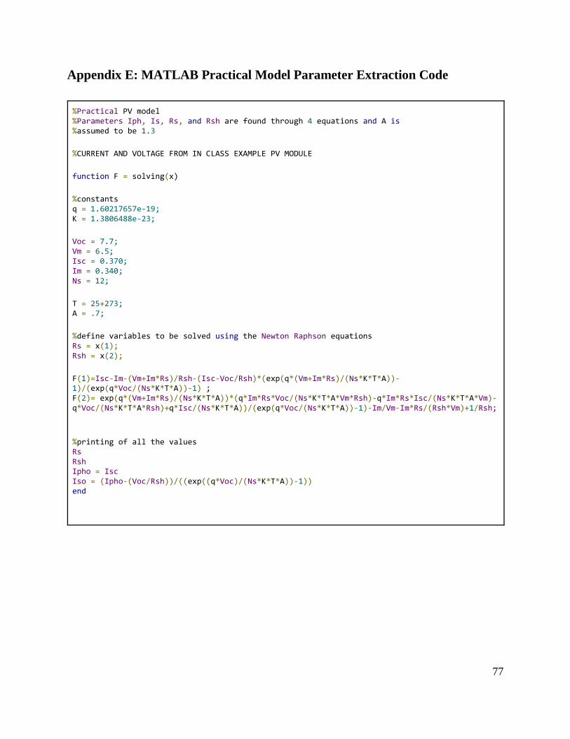
77
Appendix E: MATLAB Practical Model Parameter Extraction Code
%Practical PV model %Parameters Iph, Is, Rs, and Rsh are found through 4 equations and A is %assumed to be 1.3 %CURRENT AND VOLTAGE FROM IN CLASS EXAMPLE PV MODULE function F = solving(x) %constants q = 1.60217657e-19; K = 1.3806488e-23; Voc = 7.7; Vm = 6.5; Isc = 0.370; Im = 0.340; Ns = 12; T = 25+273; A = .7; %define variables to be solved using the Newton Raphson equations Rs = x(1); Rsh = x(2); F(1)=Isc-Im-(Vm+Im*Rs)/Rsh-(Isc-Voc/Rsh)*(exp(q*(Vm+Im*Rs)/(Ns*K*T*A))-1)/(exp(q*Voc/(Ns*K*T*A))-1) ; F(2)= exp(q*(Vm+Im*Rs)/(Ns*K*T*A))*(q*Im*Rs*Voc/(Ns*K*T*A*Vm*Rsh)-q*Im*Rs*Isc/(Ns*K*T*A*Vm)-q*Voc/(Ns*K*T*A*Rsh)+q*Isc/(Ns*K*T*A))/(exp(q*Voc/(Ns*K*T*A))-1)-Im/Vm-Im*Rs/(Rsh*Vm)+1/Rsh;
%printing of all the values Rs Rsh Ipho = Isc Iso = (Ipho-(Voc/Rsh))/((exp((q*Voc)/(Ns*K*T*A))-1)) end
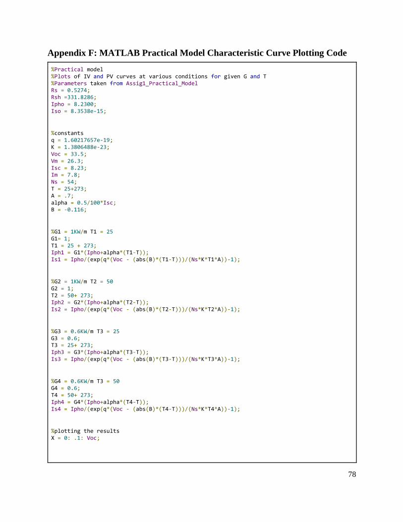
78
Appendix F: MATLAB Practical Model Characteristic Curve Plotting Code
%Practical model %Plots of IV and PV curves at various conditions for given G and T %Parameters taken from Assig1_Practical_Model Rs = 0.5274; Rsh =331.8286; Ipho = 8.2300; Iso = 8.3538e-15;
%constants q = 1.60217657e-19; K = 1.3806488e-23; Voc = 33.5; Vm = 26.3; Isc = 8.23; Im = 7.8; Ns = 54; T = 25+273; A = .7; alpha = 0.5/100*Isc; B = -0.116;
%G1 = 1KW/m T1 = 25 G1= 1; T1 = 25 + 273; Iph1 = G1*(Ipho+alpha*(T1-T)); Is1 = Ipho/(exp(q*(Voc - (abs(B)*(T1-T)))/(Ns*K*T1*A))-1);
%G2 = 1KW/m T2 = 50 G2 = 1; T2 = 50+ 273; Iph2 = G2*(Ipho+alpha*(T2-T)); Is2 = Ipho/(exp(q*(Voc - (abs(B)*(T2-T)))/(Ns*K*T2*A))-1);
%G3 = 0.6KW/m T3 = 25 G3 = 0.6; T3 = 25+ 273; Iph3 = G3*(Ipho+alpha*(T3-T)); Is3 = Ipho/(exp(q*(Voc - (abs(B)*(T3-T)))/(Ns*K*T3*A))-1);
%G4 = 0.6KW/m T3 = 50 G4 = 0.6; T4 = 50+ 273; Iph4 = G4*(Ipho+alpha*(T4-T)); Is4 = Ipho/(exp(q*(Voc - (abs(B)*(T4-T)))/(Ns*K*T4*A))-1);
%plotting the results X = 0: .1: Voc;
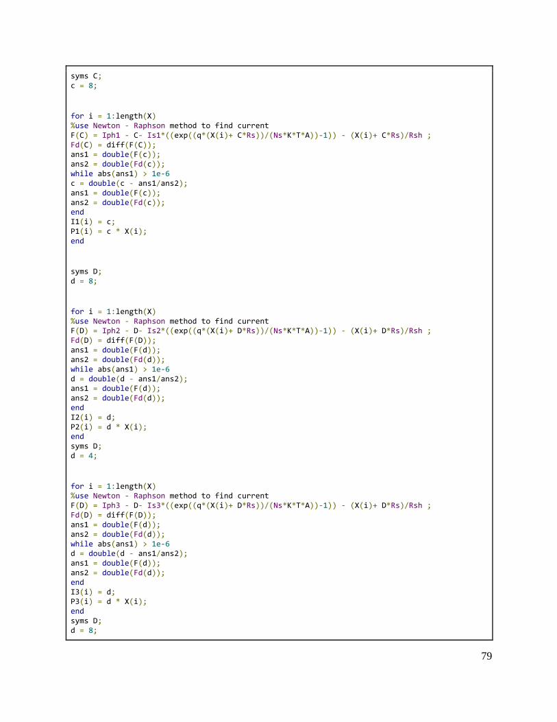
79
syms C; c = 8;
for i = 1:length(X) %use Newton - Raphson method to find current F(C) = Iph1 - C- Is1*((exp((q*(X(i)+ C*Rs))/(Ns*K*T*A))-1)) - (X(i)+ C*Rs)/Rsh ; Fd(C) = diff(F(C)); ans1 = double(F(c)); ans2 = double(Fd(c)); while abs(ans1) > 1e-6 c = double(c - ans1/ans2); ans1 = double(F(c)); ans2 = double(Fd(c)); end I1(i) = c; P1(i) = c * X(i); end
syms D; d = 8;
for i = 1:length(X) %use Newton - Raphson method to find current F(D) = Iph2 - D- Is2*((exp((q*(X(i)+ D*Rs))/(Ns*K*T*A))-1)) - (X(i)+ D*Rs)/Rsh ; Fd(D) = diff(F(D)); ans1 = double(F(d)); ans2 = double(Fd(d)); while abs(ans1) > 1e-6 d = double(d - ans1/ans2); ans1 = double(F(d)); ans2 = double(Fd(d)); end I2(i) = d; P2(i) = d * X(i); end syms D; d = 4;
for i = 1:length(X) %use Newton - Raphson method to find current F(D) = Iph3 - D- Is3*((exp((q*(X(i)+ D*Rs))/(Ns*K*T*A))-1)) - (X(i)+ D*Rs)/Rsh ; Fd(D) = diff(F(D)); ans1 = double(F(d)); ans2 = double(Fd(d)); while abs(ans1) > 1e-6 d = double(d - ans1/ans2); ans1 = double(F(d)); ans2 = double(Fd(d)); end I3(i) = d; P3(i) = d * X(i); end syms D; d = 8;
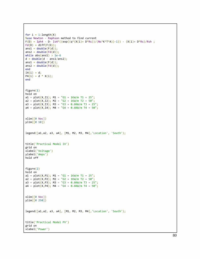
80
for i = 1:length(X) %use Newton - Raphson method to find current F(D) = Iph4 - D- Is4*((exp((q*(X(i)+ D*Rs))/(Ns*K*T*A))-1)) - (X(i)+ D*Rs)/Rsh ; Fd(D) = diff(F(D)); ans1 = double(F(d)); ans2 = double(Fd(d)); while abs(ans1) > 1e-6 d = double(d - ans1/ans2); ans1 = double(F(d)); ans2 = double(Fd(d)); end I4(i) = d; P4(i) = d * X(i); end
figure(1) hold on a1 = plot(X,I1); M1 = "G1 = 1KW/m T1 = 25"; a2 = plot(X,I2); M2 = "G2 = 1KW/m T2 = 50"; a3 = plot(X,I3); M3 = "G3 = 0.6KW/m T3 = 25"; a4 = plot(X,I4); M4 = "G4 = 0.6KW/m T4 = 50";
xlim([0 Voc]) ylim([0 10])
legend([a1,a2, a3, a4], [M1, M2, M3, M4],'Location', 'South');
title('Practical Model IV') grid on xlabel('Voltage') ylabel('Amps') hold off
figure(2) hold on a1 = plot(X,P1); M1 = "G1 = 1KW/m T1 = 25"; a2 = plot(X,P2); M2 = "G2 = 1KW/m T2 = 50"; a3 = plot(X,P3); M3 = "G3 = 0.6KW/m T3 = 25"; a4 = plot(X,P4); M4 = "G4 = 0.6KW/m T4 = 50";
xlim([0 Voc]) ylim([0 250])
legend([a1,a2, a3, a4], [M1, M2, M3, M4],'Location', 'South');
title('Practical Model PV') grid on xlabel('Power')
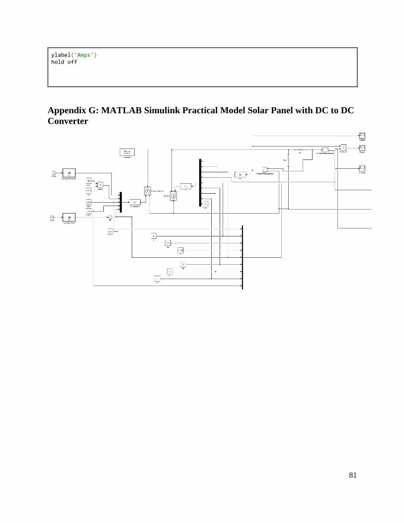
81
ylabel('Amps') hold off
Appendix G: MATLAB Simulink Practical Model Solar Panel with DC to DC
Converter
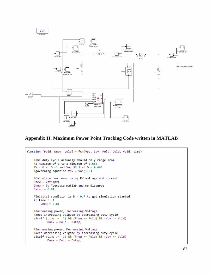
82
Appendix H: Maximum Power Point Tracking Code written in MATLAB
function [Pold, Dnew, Vold] = fcn(Vpv, Ipv, Pold, Dold, Vold, time) %The duty cycle actually should only range from %a maximum of 1 to a minimum of 0.665 %V = 0 at D =1 and Voc 33.5 at D = 0.665 %governing equation Vpv = Vo*(1-D) %Calculate new power using PV voltage and current Pnew = Vpv*Ipv; Dnew = 0; %because matlab and me disagree Dstep = 0.01; %Initital condition is D = 0.7 to get simulation started if time < .1 Dnew = 0.8; %Increasing power, Increasing Voltage %keep increasing volgate by decreasing duty cycle elseif (time >= .1) && (Pnew >= Pold) && (Vpv >= Vold) Dnew = Dold - Dstep; %Increasing power, Decreasing Voltage %keep decreasing volgate by increasing duty cycle elseif (time >= .1) && (Pnew >= Pold) && (Vpv <= Vold) Dnew = Dold + Dstep;
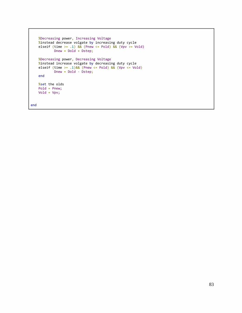
83
%Decreasing power, Increasing Voltage %instead decrease volgate by increasing duty cycle elseif (time >= .1) && (Pnew <= Pold) && (Vpv >= Vold) Dnew = Dold + Dstep; %Decreasing power, Decreasing Voltage %instead increase volgate by decreasing duty cycle elseif (time >= .1)&& (Pnew <= Pold) && (Vpv <= Vold) Dnew = Dold - Dstep; end %set the olds Pold = Pnew; Vold = Vpv; end
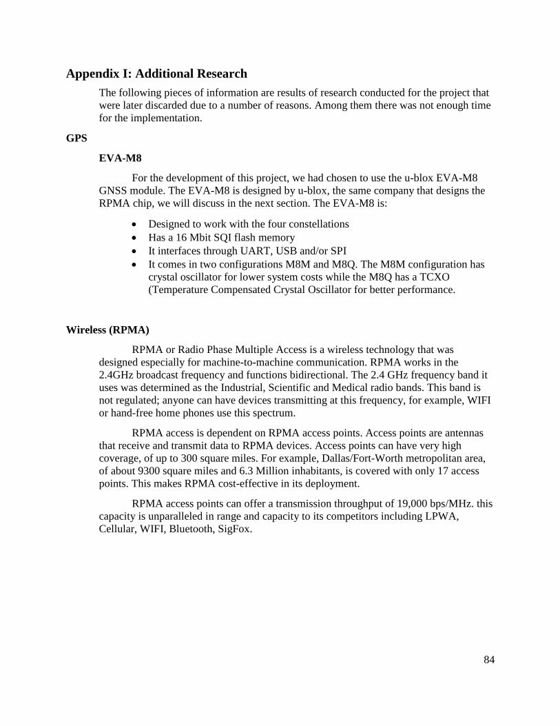
84
Appendix I: Additional Research
The following pieces of information are results of research conducted for the project that
were later discarded due to a number of reasons. Among them there was not enough time
for the implementation.
GPS
EVA-M8
For the development of this project, we had chosen to use the u-blox EVA-M8
GNSS module. The EVA-M8 is designed by u-blox, the same company that designs the
RPMA chip, we will discuss in the next section. The EVA-M8 is:
Designed to work with the four constellations
Has a 16 Mbit SQI flash memory
It interfaces through UART, USB and/or SPI
It comes in two configurations M8M and M8Q. The M8M configuration has
crystal oscillator for lower system costs while the M8Q has a TCXO
(Temperature Compensated Crystal Oscillator for better performance.
Wireless (RPMA)
RPMA or Radio Phase Multiple Access is a wireless technology that was
designed especially for machine-to-machine communication. RPMA works in the
2.4GHz broadcast frequency and functions bidirectional. The 2.4 GHz frequency band it
uses was determined as the Industrial, Scientific and Medical radio bands. This band is
not regulated; anyone can have devices transmitting at this frequency, for example, WIFI
or hand-free home phones use this spectrum.
RPMA access is dependent on RPMA access points. Access points are antennas
that receive and transmit data to RPMA devices. Access points can have very high
coverage, of up to 300 square miles. For example, Dallas/Fort-Worth metropolitan area,
of about 9300 square miles and 6.3 Million inhabitants, is covered with only 17 access
points. This makes RPMA cost-effective in its deployment.
RPMA access points can offer a transmission throughput of 19,000 bps/MHz. this
capacity is unparalleled in range and capacity to its competitors including LPWA,
Cellular, WIFI, Bluetooth, SigFox.

85
Figure 42 – Wireless Technologies Comparison
Access Point
In order to receive the signal that the RPMA module sends there needs to be an access
point. This access point are sold and/or rented by Ingenu, a company that specializes in
RPMA technology. For this project we are seeking to obtain an acess point from Ingenu
and place it on the WPI campus. Hence allowing for the development of other RPMA
technologies.
RPMA Module - NANO S-100
The Nano S-100 RPMA module will be used in our device to transmit the data to the
access point. The NANO S-100 has a 4-wire SPI interface. This module displays very
low power consumption, for applications needing 10 years or longer battery life. It can
transmit up to 100 kB daily.
Microcontroller
For a microcontroller we have chosen the TI - MSP430FR4133. For the development
phase, we will be using the Launchpad format of this microcontroller, later on we expect
to create a PCB board with the microcontroller. The MSP430FR4133 features:
16-bit MCU
16 kB of nonvolatile FRAM
10-channel 10-bit ADC
Serial Interfaces (SPI, UART, I2C)
This microcontroller is suited to handle all of the different components in our design. We
will be using five ADC channels, one for each SPEC sensor. UART interface for the PM
Sensor. Then the SPI interface to communicate with the RPMA module (Nano S-100).
And last I2C for the GNSS module (EVA-M8M).