1

1. Toolbox: SOFTWARE TOOL FOR SOLAR RADIATION AND SHADING LOSSES CALCULATIONS

1.1. Description of the tool / methodology of the tool The software tool developed by the Solar Energy Institute of the Technical University of Madrid performs solar radiation calculations and losses due to shadows casted over a given surface by nearby obstacles. On urban environments, obstacles can be located relatively close to solar installations generator and, therefore, shading losses might a significant impact on the performance of building integrated solar systems. Estimation of shading losses requires two sets of data as inputs:

Obstacle profile seen by the solar system under study. It is common practice to describe obstacles in terms of azimuth and elevation (polar coordinates): azimuth and elevation. In this software tool three possibilities to enter this data are provided, as explained below.

Solar radiation over the solar generator surface. Solar radiation depends on characteristics of the solar system (orientation and slope of the solar generator surface), as well as of the geographical location (latitude and climate):

─ The user can select the required solar radiation input data (monthly averages of daily solar radiation incident on a horizontal surface, total 12 values) from a set of predefined locations from Spain/Europe/worldwide or, alternatively, enter the values corresponding to a location not included in the tool database.

─ Latitude, solar generator orientation and slope can be also adjusted by the user. The latitude is restricted to the temperate zone, from 23.5 degrees latitude to 66.5 degrees.

Solar radiation incident on the surface under study is estimated in hourly terms for a complete year and each value is linked to the corresponding position of the sun in its sunpath. By combining the obstacle profile and sun position it is possible to know at which hours during the year the generator surface is shaded t. This process is summarized graphically in Figure 1.

2

Elevación

Acimut

80

40

0

60 120-60 -120 0

20

60

a) Sunpath with radiation data

b) Obstacle profile

c) Obstacle profile and sunpath

Elevation

Azimuth

80

40

0

60 120-60-120 0

20

60

Figure 1. Methodology for shading losses estimation.

Calculation of solar energy losses is performed after splitting the estimated hourly values of irradiation incident on the solar generator into beam, diffuse and albedo components as they behave differently to shading:

─ Beam component is directional, for this component the position of the sun on the sky dome is compared with the obstacle profile every minute. The amount of minutes in every hour in which the sun is not hidden by obstacles is used to weight beam component of solar irradiation on that hour.

─ Diffuse and albedo components are not directional. Instead, they come from wide regions of the sky, the whole dome for diffuse component and a narrow band over the horizon for albedo. These components are weighted by the fraction of the solid angle of their respective region that is covered by obstacles.

3

─ The effective ─taking into account shading losses─ global irradiation incident on the solar generator surface is, simply, the sum of the individual components.

The tool gives the user three different ways of defining the obstacle profile of the solar generator:

Self-inflicted shading on a generator arranged in parallel rows over a horizontal surface (see Figure 2).

Self-inflicted shading on a generator arranged in parallel rows over a vertical surface (see Figure 3).

Obstacle definition from rectangular coordinates of all relevant obstacle points relative to generator surface or the point from which the shading analysis is performed.

Figure 2. Self-shading between rows for a horizontally arranged solar collector.

Figure 3. Self-shading between rows for a vertically arranged solar collector.

1.2. Outcomes of the tool The results of the analysis performed by the tool can be displayed on the computer screen or stored in files. On screen, the user can visualize the following information:

4

Annual summary. Annual values of irradiation, with and without considering shading losses, are shown. Values are given for global irradiation as well as for separate components.

Monthly results. Monthly averages of solar irradiation are shown on a bar chart. Both cases, with and without shading losses, are shown together. This chart can be stored as an image.

Sunny hours. A chart shows for every hour how many days in a given month are free of shadows. This chart can be stored as an image also.

Apart from the cases already mentioned, graphic files of monthly results and sunny hours, the following options are available to the user to store information in files:

Text files. Monthly and hourly values are stored in text plain files. The user can choose the information stored in the file: with shading losses, without them or both. Global, beam, diffuse and albedo components of irradiation are stored in all cases.

Obstacle profile. The obstacle profile used in the analysis can be stored so it is possible to use it on future sessions.

Obstacle profile as image. Obstacle profiles can be stored as images so they can be included, for example, in reports.

1.3. Assessment of the tool

1.3.1. Advantages / Disadvantages Advantages of the tool are:

Simple and quick to use. Estimation of shading losses on an hourly basis, which improves result precision

and allows the analysis to be performed on different time frames (hourly, monthly, annual).

Disadvantages of the tool:

The software only allows the definition of opaque obstacles. Obstacles that don’t block completely sunlight, such as scarce trees, cannot be defined. The definition of obstacles which exhibit seasonal behaviour throughout the year, e.g. deciduous tress, is also not possible.

The tool only estimates shading losses for solar irradiation. Assessment on the impact of shading losses in the performance of solar systems, active or passive, must be performed externally to the tool.

1.4. Examples A building located in Vitoria-Gasteiz has been chosen to illustrate the use of the software tool. Shading over a façade element and a roof element have been analyzed.

1.4.1. Façade element First element analyzed belongs to the façade of the building (Figure 4).

5

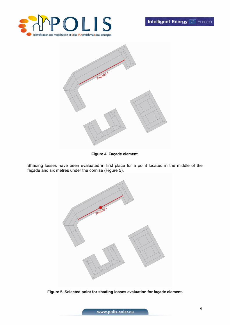
Figure 4. Façade element.

Shading losses have been evaluated in first place for a point located in the middle of the façade and six metres under the cornise (Figure 5).

Figure 5. Selected point for shading losses evaluation for façade element.

6

Once the point has been selected the following data is provided to the application:

1.4.1.1. Location and surface information Information relative to the element analyzed (building south façade) is provided to the tool. The window in Figure 6 can be accessed through:

File > Configuration The following information is provided:

Surface ─ Orientation: -28º (East) ─ Slope: 90º

Location

─ Latitude: 42.85º ─ Ground reflectivity: 0.2

Figure 6. Location and generator information for façade element.

1.4.1.2. Obstacle definition Obstacles are defined by entering the coordinates of every obstacle’s relevant points. First, we identify the obstacles that are susceptable of casting shadows over the façade (Figure 7):

Own building: ─ East wing ─ West wing

U-shaped building located south west Rectangular building located south east

7

Figure 7. Obstacles affecting façade element.

Once all obstacles have been identified their coordinates are provided to the tool. For this purpose, the following option must be selected:

Obstacles > Obstacle definition > Coordinates Every obstacle must be defined individually. Coordinates are always provided relative to the South according to the following criteria:

X axis represents the South-North direction. Positive values correspond to an obstacle located South of the point being analyzed.

Y axis represents the East-West direction. Positive values correspond to an obstacle located West of the point being analyzed.

Z axis represents height. Positive values correspond to an obstacle above the point being analyzed.

Both wings of the building to which the façade under analysis belongs, and the façade itself, are described in first place. Table 1 shows the coordinates describing these elements. All values are given in metres.

8

Element Point X coord. Y coord. Z coord.

East wing 1 -15.78 -29.68 0 2 -15.78 -29.68 9.25 3 -5.02 -35.39 9.25 4 -5.02 -35.39 0 West wing 1 16.19 30.44 0 2 16.19 30.44 6 3 24.25 36.80 6 4 48.14 24.10 6 5 48.14 24.10 0 Façade 1 16.19 30.44 0 2 16.19 30.44 6 3 -15.78 -29.68 6 4 -15.78 -29.68 0

Table 1. Coordinates describing obstacles belonging to the building.

The process of providing coordinates for the east wing of the building is shown in Figure 8.

Figure 8. East wing coordinates input.

9

Alter clicking Ok, the element is incorporated into the obstacle profile in the application main window (Figure 9).

Figure 9. Obstacle profile depicting the east wing element.

The rest of elements in Table 1 are incorporated to the obstacle profile in the same way (Figure 10).

10

Figure 10. Obstacle profile after incorporating all elements belonging to the building: east

wing, west wing and façade.

The process is repeated for all obstacles which block radiation: the south-west building and the south-east building. Element Point X coord. Y coord. Z coord.

South-west building 1 48.30 -18.96 0 2 48.30 -18.96 3.68 3 53.53 -9.12 3.68 4 53.53 -9.12 0 5 65.99 14.30 0 6 65.99 14.30 3.58 7 71.06 23.84 3.58 8 71.06 23.84 0 South-east building 1 41.82 -39.68 0 2 41.82 -39.68 4.36 3 39.63 -43.79 4.36 4 39.63 -43.79 7.38 5 29.64 -62.59 7.38

11

6 29.64 -62.59 4.42 7 27.75 -66.14 4.42 8 27.75 -66.14 0

Table 2. Coordinates describing obstacles placed to the south of the building.

The resulting obstacle profile after adding all elements previously identified as obstacles is shown in Figure 11.

Figure 11. Full obstacle profile for façade element.

It is possible to visualize the sunpath over the obstacle profile by selecting in the main window the following option ():

Visualization > Sunpath

12

Figure 12. Obstacle profile with superimposed sunpath for façade element.

1.4.1.3. Irradiation estimation Irradiation is estimated in the window in Figure 13, which is opened through the following option in the main menu:

Energy > Estimate radiation In the Estimate radiation window the user can provide to the software the average value of daily irradiation for every month. By default, the latitude provided in the configuration window (Figure 6) is used. However, this value can be modified here. The orientation and slope of the surface will be the ones defined in the configuration step. The software tool is provided with a file containing monthly averages and latitude values for a set of predefined locations. The Select location button opens a new window (Figure 14) in which is possible to select one of these predefined locations. Clicking Ok in this window loads the values of the selected location in the Estimate radiation window.

13

Figure 13. Window for irradiation estimation.

Finally, the effective irradiation on the point under analysis, located in the middle of the façade and six metres under the cornise, is estimated by selecting Ok in the Estimate radiation window. The main window shows a summary of the results: the effective annual irradiation is 848 kWh/m2. This means that 11.8% of the total irradiation is lost compared to what a surface tilted 90º and oriented 28º to the East would receive during a year in Vitoria-Gasteiz if no obstacles were present. These losses correspond to the point for which the obstacle profile (Figure 10) was obtained. Shading losses will vary throughout the façade surface, however, the previously estimated value is considered representative of the whole façade.

14

Figure 14. Window for selecting a predefined location.

15

Figure 15. Detail of application main window after estimating irradiation.

1.4.2. Roof element A roof element from the same building has been also analyzed (Figure 16).

16

Figure 16. Roof element.

Shading losses are evaluated for the roof lowest point, next to the cornise ().

Figure 17. Selected point for shading losses evaluation for roof element.

After selecting the point, it is necessary to provide all relevant information to the tool.

1.4.2.1. Location and surface information

17

Location and surface information is provided through the following option:

File > Configuration The following information () is provided:

Surface ─ Orientation: -28º (East) ─ Slope: 30º

Location

─ Latitude: 42.85º ─ Ground reflectivity: 0.2

The value of 30º for slope has been selected because is the closest from the following: 15º, 30º, 45º or 32º, which corresponds to a flat roof with auxiliary structures.

Figure 18. Location and generator information for roof element.

1.4.2.2. Obstacle definition The first step is the identification of all obstacles that can cast shadows over the roof (Figure 7). For the roof element, only the own building east wing and the building located south-east cast shadows. The west wing and the south-western building highest point is lower than the roof element and, therefore, they don’t cast shadows over the roof. The coordinates of the relevant points of the identified obstacles are presented in Table 3. Element Point X coord. Y coord. Z coord.

East wing 1 -4.53 -35.66 0 2 -4.53 -35.66 2.89 3 -16.78 -29.15 2.89 4 -16.78 -29.15 5.52 5 -24.66 -24.95 5.52

18

6 -24.66 -24.95 2.89 7 -31.04 -21.56 2.89 8 -31.04 -21.56 0 South-east building 1 37.13 -42.46 0 2 37.13 -42.46 1.38 3 27.14 -61.26 1.38 4 27.14 -61.26 0

Table 3. Coordinates describing obstacles affecting roof element.a

Once the obstacles have been identified they are input in the tool through:

Obstacles > Obstacle definition > Coordinates The resulting obstacle profile, together with the sunpath, is presented in Figure 19.

Figure 19. Obstacle profile with superimposed sunpath for roof element.

a The point chosen for roof element analysis is not coincident – they are not in the same perpendicular - with the point chosen for façade element analysis. Therefore, the X and Y coordinates of the same obstacle in both cases differ.

19

1.4.2.3. Irradiation estimation The Estimate radiation window is opened through:

Energy > Estimate radiation The information provided by default, which corresponds to Vitoria-Gasteiz, is used to estimate irradiation and shading losses. The application main window shows a summary of the results (). The shading losses over one year are 0,3%. Of a total available energy of 1435 kWh/m2 only 4 kWh/m2 are lost due to shadows casted by obstacles.

Figure 20. Detail of application main window after estimating irradiation.

The aforementioned value, 0.4%, represent losses for the point marked in Figure 17. Shading losses will vary throughout the roof, as it was the case with the façade element, but this estimated value can be considered representative of the whole roof.

1.5. Literature Previous versions of this software tool and its associated methodology have been described in the following communications: [1] Masa D, Caamaño-Martin E, Calvo-Fernández M. “Estimation of shading effects using digital tools”. Proceedings of the 22nd European Photovoltaic Solar Energy Conference 2007, Milan.

20

[2] Masa D, Caamaño-Martin E. “Improved Methodology for System Performance Analysis”. Proceedings of the 24th European Photovoltaic Solar Energy Conference 2009, Hamburg. [3] Masa D, Caamaño-Martin E. “Metodología mejorada para estimar la producción de sistemas fotovoltaicos con integración arquitectónica”. Proceedings of the 1st Congress on Distributed Generation 2009, Madrid. [4] Caamaño E, Higueras E (Editors). “Aplicación de la energía solar fotovoltaica desde la escala urbanística”. Mairea Libros: Madrid, 2010; pp. 133.