1

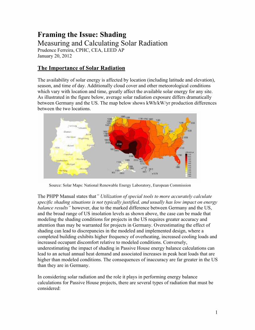
Framing the Issue: Shading Measuring and Calculating Solar Radiation Prudence Ferreira, CPHC, CEA, LEED AP January 20, 2012 The Importance of Solar Radiation The availability of solar energy is affected by location (including latitude and elevation), season, and time of day. Additionally cloud cover and other meteorological conditions which vary with location and time, greatly affect the available solar energy for any site. As illustrated in the figure below, average solar radiation exposure differs dramatically between Germany and the US. The map below shows kWh/kW/yr production differences between the two locations.

Source: Solar Maps: National Renewable Energy Laboratory, European Commission The PHPP Manual states that” Utilization of special tools to more accurately calculate specific shading situations is not typically justified, and usually has low impact on energy balance results” however, due to the marked difference between Germany and the US, and the broad range of US insolation levels as shown above, the case can be made that modeling the shading conditions for projects in the US requires greater accuracy and attention than may be warranted for projects in Germany. Overestimating the effect of shading can lead to discrepancies in the modeled and implemented design, where a completed building exhibits higher frequency of overheating, increased cooling loads and increased occupant discomfort relative to modeled conditions. Conversely, underestimating the impact of shading in Passive House energy balance calculations can lead to an actual annual heat demand and associated increases in peak heat loads that are higher than modeled conditions. The consequences of inaccuracy are far greater in the US than they are in Germany. In considering solar radiation and the role it plays in performing energy balance calculations for Passive House projects, there are several types of radiation that must be considered:

2

1. Direct Beam Radiation: The solar radiation that travels through the atmosphere in a straight line to the surface of the earth and objects on the earth is known as direct beam radiation. Because the rays of direct beam radiation are all travelling in the same direction, an object can block them all at once. Shadows are created only when direct radiation is blocked. Beam radiation may be up to 80Wm²

2. Diffuse Solar Radiation: As solar radiation passes from the sun through the

earth’s atmosphere, a portion of the energy is scattered by molecules, clouds, other aerosols and particles of dirt. The portion of the solar radiation that is scattered in the atmosphere but has still made it down to the surface of the earth is known as diffuse solar radiation or sky radiation. Diffuse radiation varies according to sky conditions and location but may be around 300Wm².

3. Some solar radiation strikes the earth or is reflected by surrounding surfaces. This

is called reflected radiation. Light colored surfaces reflect more than dark ones. The reflectivity of a surface is expressed as albedo, measured as percent of light reflected. Asphalt reflects about 4% of the light that strikes it and a lawn about 25%. An exception is in very snowy conditions, which can sometimes raise the percentage of reflected radiation quite high. Fresh snow reflects 80 to 90% of the radiation striking it. In Fairbanks, Alaska, USA (64.5° North) there is still snow on the ground in April and May and the reflected radiation portion of the total radiation can be 25%. Reflected radiation is also included in the diffuse solar radiation category.

4. Global Solar Radiation aka Global Insolation: Together, the sum of the direct

beam and diffuse and reflected solar radiation make up the global solar radiation (total solar radiation) falling on a horizontal surface.

Further distinction of solar radiation can be made to account for Angle of Incidence. The angle at which solar radiation strikes glass has a significant impact on the amount of heat transmitted. An angle of incidence of 0 occurs when the sun’s position is perpendicular to the glass. The PHPP describes the angle of incidence with a Θ-value for a window placed horizontally, for example a skylight, the Θ=0°. For a vertically placed window, the angle of incidence is 90° For standard clear single pane glass with a SHGC of 0.86 and a 0° angle of incidence, 86% of solar heat is transmitted. As the angle increases, more solar radiation is reflected, less is transmitted. Solar heat transmission through the glazing falls sharply once the angle of incidence exceeds 55°.

Also, as the angle of incidence increases, the effective area of exposure to solar radiation reduces. So, the same window can have hugely different solar gain, depending on the angle of incidence. The angle of incidence is influenced by the position of the sun according to location, season and time of day and the orientation of the glazing.

3

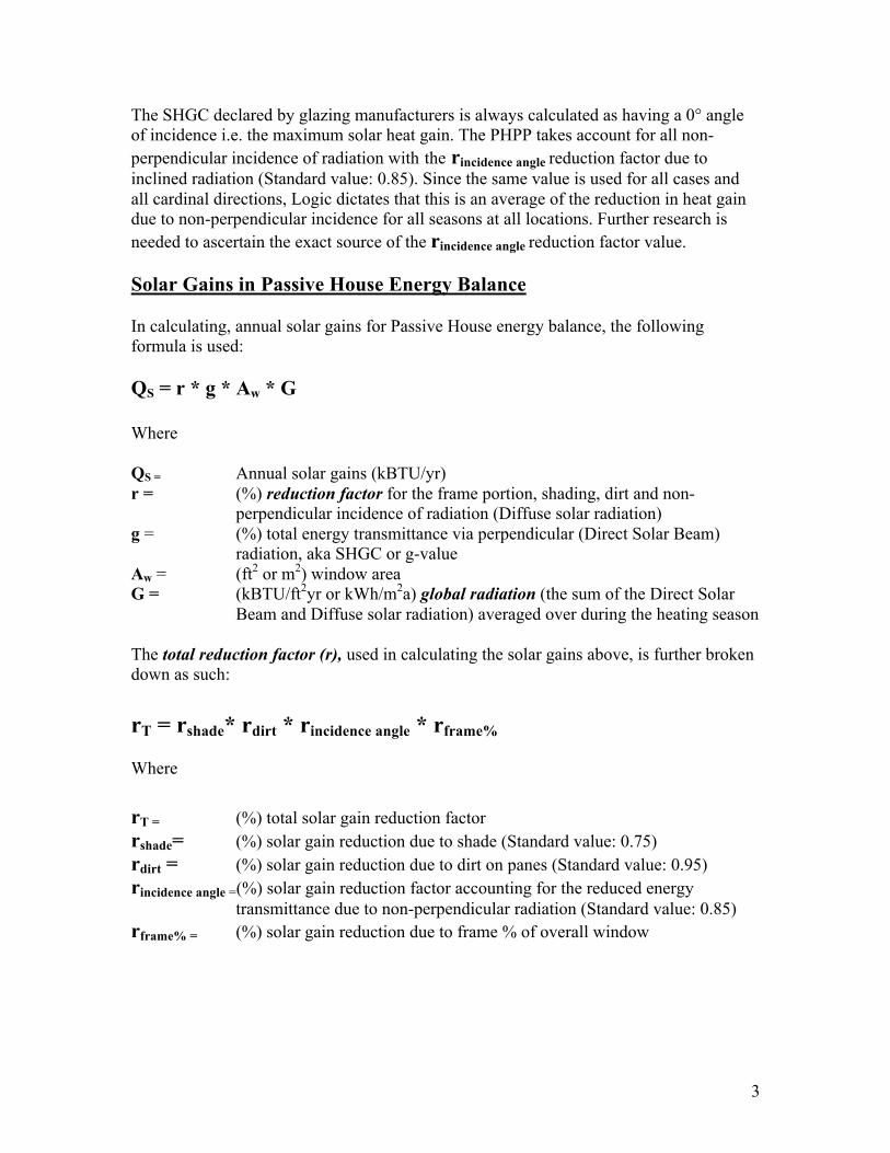
The SHGC declared by glazing manufacturers is always calculated as having a 0° angle of incidence i.e. the maximum solar heat gain. The PHPP takes account for all non-perpendicular incidence of radiation with the rincidence angle reduction factor due to inclined radiation (Standard value: 0.85). Since the same value is used for all cases and all cardinal directions, Logic dictates that this is an average of the reduction in heat gain due to non-perpendicular incidence for all seasons at all locations. Further research is needed to ascertain the exact source of the rincidence angle reduction factor value. Solar Gains in Passive House Energy Balance In calculating, annual solar gains for Passive House energy balance, the following formula is used: QS = r * g * Aw * G Where QS = Annual solar gains (kBTU/yr) r = (%) reduction factor for the frame portion, shading, dirt and non-

perpendicular incidence of radiation (Diffuse solar radiation) g = (%) total energy transmittance via perpendicular (Direct Solar Beam)

radiation, aka SHGC or g-value Aw = (ft2 or m2) window area G = (kBTU/ft2yr or kWh/m2a) global radiation (the sum of the Direct Solar

Beam and Diffuse solar radiation) averaged over during the heating season The total reduction factor (r), used in calculating the solar gains above, is further broken down as such: rT = rshade* rdirt * rincidence angle * rframe% Where rT = (%) total solar gain reduction factor rshade= (%) solar gain reduction due to shade (Standard value: 0.75) rdirt = (%) solar gain reduction due to dirt on panes (Standard value: 0.95) rincidence angle =(%) solar gain reduction factor accounting for the reduced energy

transmittance due to non-perpendicular radiation (Standard value: 0.85) rframe% = (%) solar gain reduction due to frame % of overall window

4

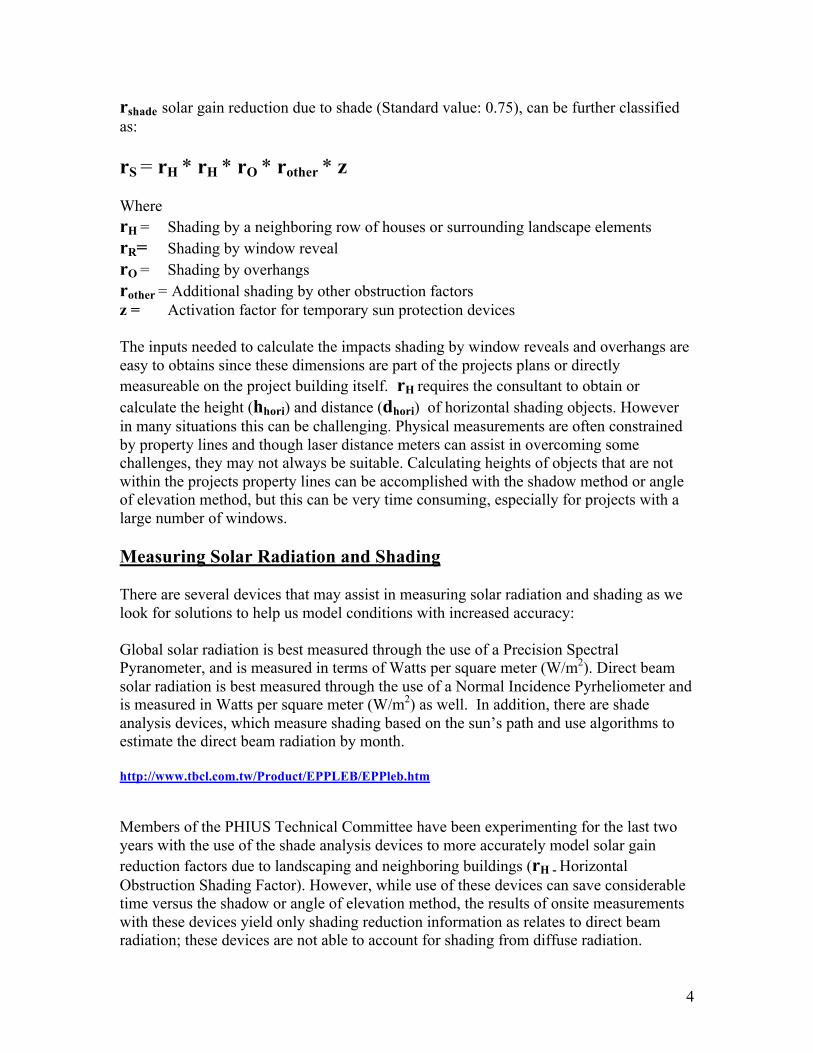
rshade solar gain reduction due to shade (Standard value: 0.75), can be further classified as: rS = rH * rH * rO * rother * z Where rH = Shading by a neighboring row of houses or surrounding landscape elements rR= Shading by window reveal rO = Shading by overhangs rother = Additional shading by other obstruction factors z = Activation factor for temporary sun protection devices The inputs needed to calculate the impacts shading by window reveals and overhangs are easy to obtains since these dimensions are part of the projects plans or directly measureable on the project building itself. rH requires the consultant to obtain or calculate the height (hhori) and distance (dhori) of horizontal shading objects. However in many situations this can be challenging. Physical measurements are often constrained by property lines and though laser distance meters can assist in overcoming some challenges, they may not always be suitable. Calculating heights of objects that are not within the projects property lines can be accomplished with the shadow method or angle of elevation method, but this can be very time consuming, especially for projects with a large number of windows. Measuring Solar Radiation and Shading There are several devices that may assist in measuring solar radiation and shading as we look for solutions to help us model conditions with increased accuracy: Global solar radiation is best measured through the use of a Precision Spectral Pyranometer, and is measured in terms of Watts per square meter (W/m2). Direct beam solar radiation is best measured through the use of a Normal Incidence Pyrheliometer and is measured in Watts per square meter (W/m2) as well. In addition, there are shade analysis devices, which measure shading based on the sun’s path and use algorithms to estimate the direct beam radiation by month. http://www.tbcl.com.tw/Product/EPPLEB/EPPleb.htm Members of the PHIUS Technical Committee have been experimenting for the last two years with the use of the shade analysis devices to more accurately model solar gain reduction factors due to landscaping and neighboring buildings (rH - Horizontal Obstruction Shading Factor). However, while use of these devices can save considerable time versus the shadow or angle of elevation method, the results of onsite measurements with these devices yield only shading reduction information as relates to direct beam radiation; these devices are not able to account for shading from diffuse radiation.

5

Diffuse solar radiation can be measured by shielding a pyranomter from the direct beam through the use of a shade. The shade however must be adjusted frequently to account for changes in the path of the sun. The shade as well presents a potential problem when accounting for the diffuse solar radiation. In order to shade the pyranometer, the shade itself must be larger than the pyranometer. This then can cast a shadow on the ground, which in turn reduces the amount of diffuse solar radiation. This approach is problematic and prone to inaccuracy. http://ir.library.oregonstate.edu/xmlui/bitstream/handle/1957/18605/Steven_and_Unsworth_Q_J_R_Met_Soc_1980_Shade-ring.pdf?sequence=1 Measurements of diffuse solar radiation are crucial for confirming radiative transfer values used in climate models. Yet, there is no international standard for diffuse solar flux. There is only an international standard for direct beam solar radiation. http://www.arm.gov/science/highlights/RMTI4/view So then what is the best method for measuring diffuse solar radiation and why do we want to measure it? Understanding the actual percentage of diffuse solar radiation is important for understanding how values for diffuse radiation should be weighted relative to direct beam solar radiation. If the diffuse radiation % of the total global radiation is not accurate, we can over- or underestimate solar gains. As stated before, global solar radiation is equal to the total solar radiation (direct solar beam and diffuse solar radiation) falling on a surface. One can derive the global solar radiation through the use of an un-shaded precision spectral pyranometer. Direct beam solar radiation can then be measured through the use of a normal incidence pyrheliometer. By computing the difference between the global solar radiation measurement from the pyranometer (W/m2) and the direct beam radiation (W/m2 measurement from the pyrheliometer) the required value for diffuse solar radiation can be derived. This method is not only simpler than using a shaded pyranomter, but is also potentially more accurate as pyranometers have an absolute accuracy of about 4%. ((http://solardat.uoregon.edu/DiffuseShadeDisk.html) We have described a method for measuring diffuse solar radiation, but to perform an accurate accounting of solar gains in Passive House energy balance, diffuse solar radiation data would be required for each cardinal direction for each station generating climate data, on a monthly average at a minimum, which would require minute by minute readings of direct beam and diffuse solar radiation for at least an entire year, preferably five to thirty years. It is unrealistic to expect that project teams or the PHIUS Technical Committee and it research partners would have the bandwidth to collect this data. In addition to our need for more accurate weighting of location-specific diffuse solar radiation and direct beam solar radiation, we also need to find a device that can accurately measure diffuse radiation shading, and convey the percentage of the sky dome exposure for each window that is blocked by shading obstructions, excluding the portion that is in the direct beam radiation path.

6

Solar Radiation Data Sets In regards to the location-specific weighting of diffuse and direct beam radiation, one would expect historical data to exist. The search for a path forward naturally leads to an exploration of data available from our national labs and scientific institutions: NASA’s Atmospheric Science Data Center Surface Meteorology and Solar Energy site (http://eosweb.larc.nasa.gov/cgi-bin/sse/) is able to report Monthly Average Diffuse radiation Incident on a Horizontal Surface in kWh/m2/day. Below is a table for San Francisco.

The issue with this data is that it is for a horizontal rather than a vertical surface. One of the properties of diffuse irradiance, which makes it challenging to model, is that values differ when measured in different directions. This property is known as “anisotropic”. The data from this set is isotropic and does not reflect any variations due to directionality. Additionally no radiation is calculated for this dataset when the sky clearness index is below 0.3 or above 0.8. The National Renewable Energy Laboratory’s (NREL) Renewable Resource Data Center (RRDC) offers a Solar Radiation Data Manual for Buildings, otherwise known as the “NREL Bluebook”. For each of the 239 stations NREL collected information from, a data page contains a description of the station location; presents average solar radiation and illuminance values for a horizontal window and vertical windows facing north, east, south, and west; and gives average climatic conditions. NREL Bluebook calculation methodology is quoted below from its Appendix-Methodology:

Calculating Incident Solar Radiation

The incident solar radiation for a horizontal window and vertical windows facing north, east, south, and west was determined using models and hourly data from the 1961-1990 National Solar Radiation Data Base (NSRDB).

Global solar radiation. The incident global solar radiation (I) received by a surface, such as a window, is a combination of direct beam radiation (Ib), sky radiation (Is), and radiation reflected from the ground in front of the surface (It). The following equation can be used to calculate incident global solar radiation:

7

Equation (1) I = Ib cos(θ) + Is +It where θ is the incident angle of the sun's rays to the surface.

The incident angle is a function of the sun's position in the sky and the orientation of the surface. Algorithms presented by Menicucci and Fernandez (1988) were used to compute incident angles. Hourly values of direct beam solar radiation from the NSRDB were used to determine the direct beam contribution (Ib cos(θ)) for each hour. Except for the first and last daylight hour, incident angles were calculated at the midpoint of the hour. For the first and last daylight hour, incident angles were calculated at the midpoint of the period during the hour when the sun was above the horizon.

The sky radiation (Id) received by the surface was calculated for the NREL Bluebook using an anisotropic diffuse radiation model developed by Perez et al. (1990). The model determined the sky radiation striking the surface using hourly values (from the NSRDB) of diffuse horizontal and direct beam solar radiation. Other inputs to the model included the sun's incident angle to the surface, the surface tilt angle from horizontal, and the sun's zenith angle. The Perez et al. model is an improved and refined version of their original model that was recommended by the International Energy Agency for calculating diffuse radiation for tilted surfaces (Hay and McKay 1988). The following equation is the Perez et al. model for diffuse sky radiation for a surface:

Equation (2) Id = Idb [0.5 (1- F1)(1 + cosβ)+ F1 a/b + F2sin β] where Idb = diffuse solar horizontal radiation F1= circumsolar anisotropy coefficient, function of sky condition F2= horizon/zenith anisotropy coefficient, function of sky condition β = tilt of the collector from the horizontal a = 0 or the cosine of the incident angle, whichever is greater b = 0.087 or the cosine of the solar zenith angle, whichever is greater. The model coefficients F1 and F2 are organized as an array of values that are selected for use depending on the solar zenith angle, the sky's clearness, and the sky's brightness. Perez et al.(1990) describe completely the manner in which this is done. The ground-reflected radiation (It) received by a surface is assumed isotropic and is a function of the global horizontal radiation (Ib), the tilt of the surface from the horizontal (β), and the ground reflectivity or albedo (ρ). Equation (3) It = 0.5ρIb (1-cos (β)) For the data in this manual, an albedo of 0.2 was used. This albedo is a nominal value for green vegetation and some soil types. The effect of other albedo values can be determined by adding an adjustment Equation (4) Iwi = 0.5 (ρt -0.2)Ib (1-cos (β))

8

Where ρt = desired albedo Ib = monthly or yearly average from data tables for incident global horizontal radiation. Diffuse solar radiation. The incident diffuse solar radiation (Id) received by a surface is the sum of the sky radiation (Is) and the radiation reflected from the ground in front of the surface (It), both of which are considered diffuse. Equation (5) Id = Is + It

Clear-day global solar radiation. Incident clear-day global solar radiation represents the global radiation obtainable under clear skies. It was calculated as above, but using clear sky values of direct beam and diffuse horizontal solar radiation. The clear sky values of direct beam and diffuse horizontal solar radiation were modeled using METSTAT (NSRDB - Vol.2,1995), the same model used to model solar radiation for the NSRDB. Inputs to METSTAT included cloud cover values of zero; average monthly values of aerosol optical depth, precipitable water, albedo, and ozone; and the day of the month of which the solar declination equals the monthly average. Average precipitable water values were multiplied by 80% to compensate for expected clear-day precipitable water compared to the mean for all weather conditions.

While the Perez model for diffuse radiation is essentially an isotropic model with two correction factors (horizon and circumsolar brightening) to approximate for the true anisotropic nature of diffuse radiation, it is still the most widely used a respected method for approximating diffuse radiation and is recommended by the International Energy Agency. In addition, the Perez model is utilized by the Passivhaus Institut in Germany for its simulations and is sited in PHI publications, such as Passive Houses in Southwest Europe (2nd corrected edition, Jurgen Schnieders 2009). Below are charts of the NREL Bluebook data for San Francisco, which utilizes the Perez method for determining diffuse radiation.

0  100  200  300  400  500  600  700  800  

Jan   Feb  Mar  Apr  May  Jun   Jul   Aug  Sep   Oct  Nov  Dec  

(BTU/ft2/day)  

Month  

North  Average  Incident  Solar  Radiation:  SF,  CA  

North  Clear  Day  Global  

North  Average  Global  

North  Diffuse  

9

0  

500  

1000  

1500  

2000  

Jan   Feb  Mar  Apr  May   Jun   Jul   Aug  Sep   Oct   Nov  Dec  

(BTU/ft2/day)  

Month  

East  Average  Incident  Solar  Radiation:  SF,  CA  

East  Clear  Day  Global  

East  Average  Global  

East  Diffuse  

0  

500  

1000  

1500  

2000  

Jan   Feb  Mar  Apr  May  Jun   Jul   Aug  Sep   Oct  Nov  Dec  

(BTU/ft2/day)  

Month  

South  Average  Incident  Solar  Radiation:  SF,  CA  

South  Clear  Day  Global  

South  Average  Global  

South  Diffuse  

0  

500  

1000  

1500  

2000  

Jan   Feb  Mar  Apr  May  Jun   Jul   Aug  Sep   Oct  Nov  Dec  

(BTU/ft2/day)  

Month  

West  Average  Incident  Solar  Radiation:  SF,  CA  

West  Clear  Day  Global  

West  Average  Global  

West  Diffuse  

10

This radiation data presented above however does not align with the radiation data in the PHPP Climate set for San Francisco; more research is needed to understand the discrepancies. It has been suggested that the effects of diffuse radiation are “baked in” to the PHPP climate data, but further study is needed to confirm. Meteonorm, the folks who provide the datasets that serve as the basis for PHPP climate data may have some helpful information in regards to diffuse radiation as well, which the Technical Committee is pursuing. Below is the same radiation data set as above from the NREL Bluebook, showing relative percentages of diffuse radiation in relation to global anisotropic radiation and global horizontal radiation. Again below, see NREL Bluebook Solar Radiation Data for San Francisco:

Where the percentage of diffuse radiation for the North as compared to: Horizontal Clear Day Global = 20.11% North Clear Day Global = 92.31% North Average Global = 94.74%

Where the percentage of diffuse radiation for the East as compared to: Horizontal Clear Day Global = 24.58% East Clear Day Global = 40.74% East Average Global = 54.32%

Horizontal  Clear  Day  Global  

North  Clear  Day  Global  

North  Average  Global   North  Diffuse  

Yr   1790   390   380   360  

0  

500  

1000  

1500  

2000  

(BTU/ft2/day)  

North  Average  Incident  Solar  Radiation:  SF,  CA  

Yr  

Horizontal  Clear  Day  Global  

East  Clear  Day  Global  

East  Average  Global   East  Diffuse  

Yr   1790   1080   810   440  

0  500  1000  1500  2000  

(BTU/ft2/day)  

East  Average  Incident  Solar  Radiation:  SF,  CA  

Yr  

11

Where the percentage of diffuse radiation for the South as compared to: Horizontal Clear Day Global = 24.58% South Clear Day Global = 40.74% South Average Global = 54.32%

Where the percentage of diffuse radiation for the South as compared to: Horizontal Clear Day Global = 24.58% South Clear Day Global = 40.74% South Average Global = 54.32% As we have discussed and can see from the information above, diffuse radiation varies depending on the direction of the measurement. The logical conclusion is that for improved accuracy of calculation, one would include an anisotropic diffuse radiation reduction factor for the global radiation to account for the percentage of non-perpendicular radiation from each cardinal direction. Reflected Radiation and Albedo The situation around diffuse radiation is further complicated by the fact that the PHPP actually does not include ground-reflected radiation in its non-perpendicular radiation reduction factor, as the Perez model does, but instead accounts for it separately. The

Horizontal  Clear  Day  Global  

South  Clear  Day  Global  

South  Average  Global   South  Diffuse  

Yr   1790   1460   1080   470  

0  500  1000  1500  2000  

(BTU/ft2/day)  

South  Average  Incident  Solar  Radiation:  SF,  CA  

Yr  

Horizontal  Clear  Day  Global  

West  Clear  Day  Global  

West  Average  Global   West  Diffuse  

Yr   1790   1080   900   450  

0  500  1000  1500  2000  

(BTU/ft2/day)  

West  Average  Incident  Solar  Radiation:  SF,  CA  

Yr  

12

inputs for the calculation of ground-reflected radiation are the same for the PHPP as in the Perez model:

The ground-reflected radiation (It) received by a surface is assumed isotropic and is a function of the global horizontal radiation (Ib), the tilt of the surface from the horizontal (β), and the ground reflectivity or albedo (ρ).

It = 0.5ρIb (1-cos (β)) However, the albedo factor the PHPP uses is 0.106, while the Perez model uses 0.2, a nominal albedo value for green vegetation and some soil types. Most land areas are in an albedo range of 0.1 to 0.4. The average albedo of the Earth is about 0.3, and fresh snow has an albedo between 0.80 – 0.90. The higher the albedo, the whiter or more reflective a surface is. The PHPP albedo factor 0.106 is roughly equivalent to mid-aged asphalt. Does changing the albedo make a difference, and if so how much of a difference? An experiment was performed with the Kerr Avenue PHPP file, whereby the albedo value of 0.106 (used for all PHPP climate sets globally), was increased to 0.2, 0.5, 0.7 and 0.9, and then down to 0.01 and 0.001 respectively. These shifts yielded the following results on the Cooling Load worksheet:

Where the albedo factor = 0.106, the solar gains resulting from the sum of opaque areas = 1276 BTU/hr and the cooling load = 16010 BTU/hr Where the albedo factor = 0.2, the solar gains resulting from the sum of opaque areas = 1268 BTU/hr and the cooling load = 16002 BTU/hr Where the albedo factor = 0.5, the solar gains resulting from the sum of opaque areas = 1240 BTU/hr and the cooling load = 15973 BTU/hr Where the albedo factor = 0.7, the solar gains resulting from the sum of opaque areas = 1235 BTU/hr and the cooling load = 15969 BTU/hr Where the albedo factor = 0.8, the solar gains resulting from the sum of opaque areas = 1255 BTU/hr and the cooling load = 15989 BTU/hr Where the albedo factor = 0.9, the solar gains resulting from the sum of opaque areas = 1312 BTU/hr and the cooling load = 16046 BTU/hr To explore the extremes of shifting the albedo factor: Where the albedo factor = 0.99, the solar gains resulting from the sum of opaque areas = 2132 BTU/hr and the cooling load = 16866 BTU/hr Where the albedo factor = 0.9999, the solar gains resulting from the sum of opaque areas = 90580 BTU/hr and the cooling load = 105314 BTU/hr and the warning” Caution: Large daily temperature swing. Consideration of daily average

13

cooling load is not sufficient. Reduce solar load! Heading in the opposite direction, where the albedo factor = 0.01 the solar gains resulting from the sum of opaque areas = 1283 BTU/hr and the cooling load = 16017 BTU/hr

Where the albedo factor = 0.001 the solar gains resulting from the sum of opaque areas = 1284 BTU/hr and the cooling load = 16018 BTU/hr

Conclusions These are the findings to date with respect to the current challenges of accurately measuring the impacts of shading on direct beam, diffuse and reflected solar radiation, and inputting the data into the PHPP in the manner that will most accurately account for its impacts:

1. The measurement of diffuse radiation can be accomplished with the combined use of a Precision Spectral Pyranometer and a Normal Incidence Pyrheliometer, but an accurate dataset for a given location would require minute-by-minute readings for at least a year, preferably five to thirty years.

2. Shade analysis devices measure shading impacts for direct beam radiation only and do not account for the effect of shading on diffuse radiation.

3. Diffuse Radiation is anisotropic and varies by location, it is necessary to assess whether the PHPP has the correct weighting for diffuse relative to direct beam radiation for all North American locations.

4. While the Perez model for diffuse radiation includes reflected radiation (with a default albedo of 0.2) in its diffuse radiation values, the PHPP handles reflected radiation separately and uses an albedo of 0.106 for all locations globally.

5. Modifying the PHPP albedo factor produces changes in the cooling load; For albedo values between 0.2 and 0.7 as the albedo increases, the cooling load associated with the “sum of opaque areas” decreases. For values between 0.8 and 0.999, as the albedo increases, the cooling load associated with the “sum of opaque areas” also increases.

Further research and work to be completed by the Technical Committee on these matters is as follows:

1. Locate a dataset or find an organization to create diffuse radiation datasets for N. American locations to guide the determination of appropriate diffuse radiation and direct beam radiation weighting for these locations.

2. Locate a device capable of accurately measuring diffuse radiation shading, and/or a methodology for utilizing direct beam shading measurements devices and correcting for the diffuse radiation shading manually or through calculations.

3. Further investigate the impacts of reflected radiation and determine whether and in which situations the PHPP albedo factor should be modified to account for the albedo of the project site.

4. Create and publish protocols for incorporating the outputs of various shading device readings for use in the rHHorizontal Obstruction Shading Factor.

14

References

ASHRAE (1993). 1993 ASHRAE Handbook: Fundamentals. Atlanta, GA: American Society of Heating, Refrigerating and Air-Conditioning Engineers, Inc.

Colgan, R.; Wiltse, N.; Lilly, M.; LaRue, B.; Egan, G. (2010). Performance of Photovoltaic Arrays - Cold Climate Housing Research Research Center: CCHRC Snapshot RS 2010-01.

Duffie, J.A.; Beckman, W.A. (1991). Solar Engineering of Thermal Processes. 2nd Edition. New York: John Wiley & Sons,Inc.

Hay, J.E.; McKay, D.C.(1988). Final Report IEA Task IX-Calculation of Solar Irradiances for Inclined Surfaces: Verification of Models Which Use Hourly and Daily Data. International Energy Agency Solar Heating and Cooling Programme.

Iqbal, M. (1983). An Introduction to Solar Radiation. New York: Academic Press, Inc.

Linacre, E. (1992). Climate Data and Resources. New York: Routledge.

Menicucci, D, ;Fernendez, J.P. (1988). User's Manual for PVFORM: A Photovoltaic System Simulation Program for Stand-Alone and Grid-Interactive Applications. SAND85-0376, Albuquerque, NM: Sandia National Laboratories.

NSRDB-Vol.2 (1995). Final Technical Report: National Solar Radiation Data Base (1961-1990). NREL/TP-463-5784, Golden, CO: National Renewable Energy Laboratory.

Perez, R.; Ineichen, P.; Seals ,R.; Michalsky, J.; Stewart, R. (1990). "Modeling Daylight Availability and Irradiance Components from Direct and Global Irradiance.” Solar Energy, 44(5), pp.271-289.