NBER WORKING PAPER SERIES

SOCIAL CAPITAL AND URBAN GROWTH

Edward L. GlaeserCharles Redlick

Working Paper 14374http://www.nber.org/papers/w14374

NATIONAL BUREAU OF ECONOMIC RESEARCH1050 Massachusetts Avenue

Cambridge, MA 02138October 2008

We thank the Taubman Center for State and Local Government for research support. This essay waswritten in honor of Roger Bolton and his many contributions to regional economics. The views expressedherein are those of the author(s) and do not necessarily reflect the views of the National Bureau ofEconomic Research.

© 2008 by Edward L. Glaeser and Charles Redlick. All rights reserved. Short sections of text, notto exceed two paragraphs, may be quoted without explicit permission provided that full credit, including© notice, is given to the source.

Social Capital and Urban GrowthEdward L. Glaeser and Charles RedlickNBER Working Paper No. 14374October 2008JEL No. D0,H0,I0,J0,R0

ABSTRACT

Social capital is often place-specific while schooling is portable, so the prospect of migration mayreduce the returns to social capital and increase the returns to schooling. If social capital matters forurban success, it is possible that an area can get caught in a bad equilibrium where the prospect ofout-migration reduces social capital investment and a lack of social capital investment makes out-migrationmore appealing. We present a simple model of that process and then test its implications. We findlittle evidence to suggest that social capital is correlated with either area growth or rates of out-migration.We do, however, find significant differences in the returns to human capital across space, and a significantpattern of skilled people disproportionately leaving declining areas. For people in declining areas,the prospect of out-migration may increase the returns to investment in human capital, but it does notseem to impact investment in social capital.

Edward L. GlaeserDepartment of Economics315A Littauer CenterHarvard UniversityCambridge, MA 02138and NBEReglaeser@harvard.edu

Charles RedlickDepartment of EconomicsLittauer Center 200Harvard UniversityCambridge, MA 02138credlick@fas.harvard.edu

  2

I. Introduction

Should national governments engage in place-based policies that direct resources towards

declining or poor regions? Standard results in urban economics suggest that place-based

policies are unlikely to enhance economic efficiency or prudently promote equity. Unsuccessful

places are generally less productive, so directing people towards those areas may reduce national

productivity, and transfers to poor areas may well help property owners and the prosperous more

than the less fortunate.

Roger Bolton has regularly put forward a contrarian point of view that suggests a greater role for

the central government in “place-making.” This view emphasizes the value of a “sense of

place,” which can be understood as a type of location-specific social capital. Social capital may

be built through a variety of local place-making activities such as group membership and

political activism. In Section III of this paper, we present a simple model of social capital

investment where the incentives to invest decline when individuals expect to leave their current

locale.

This feedback mechanism creates the possibility of multiple equilibria. In one equilibrium,

people expect to leave and therefore invest little in social capital. Low levels of social capital

then make an area less attractive and so people do end up leaving. In a second equilibrium,

people expect to stay and so invest more in social capital. In principle, this type of multiple

equilibria story could explain why geographic mobility is so much higher in the U.S. than in

Europe (as in Spilimbergo and Ubeda, 2004). This virtuous circle holds together because the

high level of social capital investment keeps people interested in staying in the area.

This model creates a defensible rationale for government subsidy of declining areas. By

increasing the attractiveness of an area, the central government raises the probability that an

individual will want to stay in that area, which in turn increases the degree of investment in

social capital. Government support for distressed areas can be seen as a means of subsidizing the

positive externalities associated with social capital investment. In principle, it is even possible

  3

that government intervention could move the city from the bad equilibrium, where everyone

leaves and no one invests, to the good equilibrium, where people stay and invest.

While there is no doubt that theory can provide an intellectually coherent rationale for supporting

declining areas, it is less obvious that the model’s conditions for federal government support to

be beneficial are met in the real world. After all, providing incentives for geographic stability is

a more direct means of promoting social capital investment than propping up declining areas.

The home mortgage interest deduction, which promotes homeownership and reduces mobility,

can be seen as a policy meant to promote social capital (Glaeser and DiPasquale, 1999). If

human capital investments also create spillovers, and if the returns to human capital are higher

outside of declining regions, then propping up those regions will cause a reduction in human

capital investment that must be weighed against any gains from social capital investment.

After presenting our model, we turn to the data. We first note that there is a substantial

difference between cities that are in decline and cities with large out-migration probabilities.

Many quickly growing places, like Austin, Texas and Charlotte, North Carolina, have higher

emigration rates than America’s declining cities (naturally, they also have much higher in-

migration rates). In these cases, high levels of emigration do not seem to be impeding whatever

is necessary for urban success.

We then turn to the cross-city evidence on the relationship between social capital and urban

decline. Across areas, there is little clear connection between low levels of social capital

investment and either population growth or out-migration rates. While the multiple equilibria

model may have an intuitive appeal, it is not true that declining areas are particularly short on

social capital. They are, however, particularly short on human capital.

We next consider the connection between social capital and geographic mobility. People who

are more mobile do seem to invest less in social capital, but there is more question about whether

reducing the out-migration rate from an area will increase its social capital investment. A simple

cross-sectional regression that looks at the connection between forms of social capital investment

and either area-level out-migration rates or area-level decline finds little connection. This makes

  4

us question whether reducing area level decline or out-migration will, in fact, increase the level

of social capital in an area.

Finally, we turn to the connection between urban decline and human capital. There are

substantial differences across space in the returns to skill. For example, the returns to a college

degree are higher in denser places and in areas where more college graduates choose to live.

These facts suggest that the ability to move locations can increase the returns to becoming

educated in a less skilled city. It is also true that more skilled people are particularly likely to

leave declining urban areas. Propping up declining areas may reduce this exodus, which may

create positive externalities on the other residents of the declining area. However, this may also

have negative externalities on the areas that were attracting the high human capital workers. The

case for sorting policies to be efficient requires some evidence of non-linearities in human capital

externalities, and we know of no evidence supporting the existence of such non-linearities

(Glaeser and Gottlieb, 2008).

We do know, however, that the probability of finishing high school is higher in areas with higher

levels of emigration. Moreover, people with more education are more likely to flee declining

areas. This may support the view that restricting mobility out of declining areas will reduce the

incentive to invest in human capital, which could even hurt declining areas. If we are confident

about the existence of human capital externalities, but not confident about local non-linearities,

then there is likely to be a social cost from reduced human capital investment if we try to induce

people to stay in areas with low returns to human capital.

II. People vs. Place; Social Capital vs. Human Capital

Urban and regional economists have long debated the relative merits of investment by the federal

government in people or places (e.g. Winnick, 1966). Economic logic typically suggests that

person-based policies, like subsidies to education or the Low Income Housing Tax Credit,

dominate place-based policies, such as the Model Cities Program and Empowerment Zones.

Place-based policies seem poorly targeted to help poorer people. After all, plenty of people in

poorer places aren’t poor and property owners tend to benefit significantly from policies that

  5

make a particular locale more attractive. Moreover, there are many cases where place-based

thinking appears to have justified particularly wasteful infrastructure projects that yield little

social benefit to anyone.

The core theoretical tool of urban economics – the spatial equilibrium – pushes back against the

use of place-based policies as a tool for redistribution. The vital assumption of spatial

equilibrium models is that free migration across space and flexible housing prices ensure that

welfare levels are more or less equal in different areas. Central city Detroit may be poor, but it

also has low housing prices that offset that poverty. If welfare levels are more or less equal

across space, then there is no good equity rationale for redistributing income from richer places

to poorer places.

Admittedly, the distinction between place and people is often ambiguous. Many investments in

human capital, such as schools, are inherently rooted in a particular place. Moreover, even the

staunchest advocates of people-based policies accept that localities should invest in their own

places. However, the weight of economic writing has generally been against using federal

interventions to subsidize particular locations.

Roger Bolton is one of those rare economists who have intellectually defended place-making

policies. In many papers, Bolton has emphasized the enormous importance that places, or “sense

of place,” can have on people’s lives, and he is surely right to have done so. Figure 1 shows the

53 percent correlation between the share of people saying that they are either somewhat or very

happy in the General Social Survey and population growth in their metropolitan area in the

1990s. People in declining areas seem to be significantly less happy than people in areas that are

attracting new people. While this link seems to suggest the importance of place, that fact alone

does not suggest that growing areas should subsidize declining areas.

Bolton (1992) elegantly surveys the literature on people prosperity vs. place prosperity and then

offers three arguments for government policies to strengthen declining places. Bolton’s first

argument is that people who do not currently live in a declining area may like to have the option

  6

of migrating to a declining area. If the declining area is allowed to disappear, then that option

will disappear along with it.

On its own, this option value does not create a cross-jurisdictional externality. The fact that

outsiders may sometimes decide to move to an area will increase that area’s property values.

Local government policies that try to maximize those property values will make investments

recognizing the potential value of the area to outsiders. For centuries, local boosters have fought

for policies not only on the basis of their current need, but also because those policies may attract

more people to an area. There must be some added externality or coordination failure that turns

the option value of being able to move to an area into a reason to support it.

The second reason that Bolton gives for place-making policies is that there is a psychic

externality created by the economic health of a particular place. People outside that place may

have no desire to live in that place or even visit that location, but they are still better off knowing

that the place exists and is doing well. This type of argument is frequently made for subsidizing

national parks. This argument was also made for national subsidies of New Orleans after

Hurricane Katrina. It was alleged that the value of that historic city to the American national

consciousness made it reasonable to spend billions rebuilding it.

Bolton’s third argument is that taxpayers simply like supporting payments that build up

particular places. The third and second arguments are quite similar in that they both rely on

preferences for supporting particular places, and these preferences are inherently hard to observe.

Perhaps it is true that taxpayers like the idea of subsidizing inner cities and Appalachia for

immutable taste-based reasons, but this contention is obviously debatable and difficult to verify.

Moreover, it is also possible to take the view that such preferences are weak and malleable,

which makes them only moderately appropriate guides for public policy.

In this essay, we consider a fourth reason for place-based policies that is also based on Bolton’s

work: location-based externalities in human and social capital. These issues are particularly

appropriate in an essay written for Roger Bolton, since he has been a leader in bringing social

capital into regional economics (Bolton, 1992, 2003). Investments in social capital, which can

  7

be thought of as social connections and institutions, are generally thought to have significant

externalities. Individuals who set up networks or invest in clubs are generally creating benefits

for the other members of those networks and clubs, as well as for themselves. The existence of

these externalities means that the private spatial equilibrium is unlikely to be optimal.

However, the mere presence of externalities, such as human capital spillovers or agglomeration

economies, does not lead to a clear spatial policy (Glaeser and Gottlieb, 2008). Moving skilled

people from one place to another may increase the productivity of the area where skilled people

are moving to, but it will correspondingly decrease the productivity of the area that is losing

skilled people. Without a clear non-linearity in these spillovers, government policies that favor

one region or another are as likely to cause harm as good.

The standard assumptions about social capital suggest that social capital externalities are more

likely to yield a strong spatial policy conclusion. We normally assume that most social capital

investments are linked to a specific place, and that the benefits of investment are more or less

lost with migration. As a result, high out-migration rates should reduce the level of investment

in local churches, hobby groups and political clubs. If we believe that there are significant

externalities associated with these investments, then high levels of mobility will create negative

externalities by destroying an area’s “sense of place” (Bolton, 1987).

In the next section of this paper, we present a model that gives conditions under which social

capital investment creates a case for subsidizing particular places. In the model, there is always

an advantage to propping up declining regions, because this reduces mobility and increases

social capital investment. However, subsidizing a declining region will in turn have negative

effects on human capital investment if the returns to human capital are higher in growing areas.

As such, the case for place-based policies pits social capital against human capital. In Section

IV, we turn to the question of whether the conditions for subsidizing declining places are likely

to be met in the real world.

  8

III. Multiple Equilibria and Mobility

We consider a two-period model, where individuals have a first period of investment and then

choose whether to stay in their initial location or move. They can invest in their human capital

level, h, and their social capital, s. Both social and physical capital enhance individual welfare,

and in both cases there are complementarities across people.

The primary difference in the two forms of investment is that social capital is location-specific

while human capital is not. An individual who gets a college degree can take the skills that he or

she learns everywhere. An individual who invests in social connections within a specific place

cannot. In the first period, investment occurs, individuals learn their match quality with a

specific locale, and they must then decide whether or not to move to someplace else.

Utility for person i in location j in period two equals ijjijji ssVhhU ε++ )ˆ,()ˆ,( , where ih is the

human capital investment for person i and jh is the average human capital investment for all

people in location j. An individual’s place-specific social capital ijs equals is , person i’s

investment in social capital, if person i is staying in the same place that he or she grew up, or 0 if

person i has moved. The term js refers to the average social capital of individuals living in area

j. The final noise term ijε reflects person i’s idiosyncratic taste for living in this specific

community. We assume that 0)ˆ,(1 >ji hhU , 0)ˆ,(2 ≥ji hhU , 0)ˆ,(12 ≥ji hhU and that

0)ˆ,()ˆ,( 12 <+ jijiii hhUhhU , where )ˆ,( jik hhU refers to the derivative of (.,.)U with respect to its

kth argument. The same four conditions apply for the (.,.)V function, and we also assume

0)ˆ,0( =jsV .

The decisions about human capital, social capital, and mobility are made in period one to

maximize the value of:

(1) iiijjijji shssVhhU −−++ ))ˆ,()ˆ,(( εβ ,

where β represents the discount factor. We initially assume that individuals are homogeneous,

except for region-specific tastes.

  9

We first consider a particularly simple version of the model. All individuals start off in one

place, location “1,” and there is a single other location where they could move, location “2”.

Since no one begins in location 2, there is no social capital in that area. Individuals do not know

their value of 1iε before they invest in either form of capital, but they learn the value of 1iε

before choosing whether or not to migrate. The expected value of the idiosyncratic taste for the

second area equals 2ε , but the realized value is not known before migration decisions are made.

The equilibrium of the model is determined by the following equations. First, individuals who

know that they are moving will not invest in social capital. Individuals who are staying will

invest in social capital to the point where: 1),(1 =ssVβπ , where π denotes the endogenous

probability they assign to staying in location one. We let )(π∗s denote the value of s that

satisfies this equation. The human capital investment equation is that 1),(1 =hhUβ . We let ∗h denote the value of h that satisfies that equation.

Differentiation then gives us that ),(),(

),(1211

1

ssVssVssVss

+−=

∂∂

=∂∂ ∗∗

ββ

ππ . This expression includes

the fact that changes in parameter values will have both a direct and an indirect effect on social

capital investment. When it is more likely that a person will choose not to migrate, holding

everyone else’s behavior constant, this increases the returns to investing in social capital.

However, there is also a social multiplier when everyone’s probability of staying in the area

increases. Since the person’s neighbors are also investing more in social capital, this further

increases the returns to investment. This effect is incorporated by the term ),(12 ssV , which

captures the interpersonal complementarity between the two types of social capital investment.

The assumption 0),(),( 1211 <+ ssVssV ensures that the overall impact of permanence will still be

positive.

Given these two investment equations, individuals then decide whether or not to migrate when

their value of 1iε is revealed. Specifically, there will be a marginal individual, with a value of

1iε denoted ∗ε , who is indifferent between migrating and not migrating. If the expected value of

2iε is 2ε , then the value of ∗ε will satisfy ∗∗∗ −=− εε 2ˆ),( ssV , and individuals will leave only if

  10

they have a value of 1iε below 2ˆ),( ε−∗∗ ssV . If the cumulative distribution of ε is (.)F , then

the ex ante probability of leaving location one is )),(ˆ( 2∗∗− ssVF ε , which equals π−1 . The

equilibrium for the model can then be described by the complete investment equation for social

capital 1))),(ˆ(1)(,( 21 =−− ∗∗∗∗ ssVFssV εβ .

We next assume that (.,.)V and (.)F are continuously differentiable. If we also assume that

1)0,0())ˆ(1( 12 >− VF εβ , so that individuals will never choose to invest nothing in social capital,

and that for high enough values of s, 1),(1 <ssVβ , then there exists at least one point where

1))),(ˆ(1)((,( 21 =−− ∗∗∗∗ ssVFssV εβ . This then implies that there will be an odd number of

equilibria of the model, ensuring that at least one will exist.

As in Spilimbergo and Ubeda (2004), there can be more than one equilibrium of the model. For

example, if there is an equilibrium where

(2) ),(),()),(ˆ(1

)),(ˆ()),(),(( 11122

221

∗∗∗∗∗∗

∗∗∗∗∗∗ −>+

−−−

+ ssVssVssVF

ssVfssVssVε

ε

then there will exist multiple equilibria, some of which have higher levels of social capital and

mobility. For another example, suppose we assume the functional form σσ −+= 1)ˆ()ˆ,( jijjij ssvsssV . In this case, the equation becomes

∗∗∗∗

∗∗

+−

>−−

−ssss

ssVFssVf

σσσ

εε

22

2

)()1(

)),(ˆ(1)),(ˆ( . If (.)F is an exponential distribution, xe λ−−1 , then this

simplifies to ∗∗ +−

>ssss

σσσλ 2)(

)1( .

To illustrate the possibility of multiple equilibria, consider the following discrete example, where

the value of s can be either zero or one and the utility from social capital is given by ss ˆβα + for

parameters α and β . We specifically chose to assume no complementarity between individual

social capital investment and area social capital investments. We do not do this out of doubt that

  11

such complementarities exist (they surely do), but rather because the existence of such

complementarities is well known to create the potential for multiple equilibria. Our goal with

this example is to show that the potential for multiple equilibria exists even without those

complementarities, through a pure migration effect.

We ignore human capital and assume that 1iε is uniformly distributed on the interval [0, 4], and

that 2ˆ2 =ε . If an individual invests in social capital, that person will stay in the city if and only

if 2ˆ 1 >++ is εβα . The ex ante probability that an investor will stay in their city equals

4/)ˆ(5. sβα ++ , and the return to social capital investment equals α times that amount. If

( ) ( )4/)(5.14/5. βαααα ++<<+ , then there will be multiple equilibria. In one equilibrium,

the returns to investment in social capital are low because people expect to migrate. As a result,

people don’t invest in social capital and migration occurs. However, there is a second possible

equilibrium where everyone invests in social capital and mobility is low. People then stay in the

area because the level of social capital is high. This equilibrium is certainly preferable to the

high mobility, low investment equilibrium.

Figure 2 illustrates the model when α is 1.1 and β equals .9. The rising line illustrates the

return to investment in social capital, which increases with the share of the population also

investing in social capital. This increase occurs because as more people invest in social capital,

the probability of staying in the place rises, so the returns to investment also rises. The flat line

represents the cost of investment, which always equals one. The declining line shows the

decreasing share of the population who leave the area. When there is no investment, fifty

percent of the city departs; when everyone invests, everyone stays.

The figure illustrates that there is also a third equilibrium where only a portion of the population

invests and the returns to investment exactly equal the costs. This equilibrium will not be stable,

however, since if a small amount of people change their migration or investment behavior, then

the outcome will converge to one of the other two equilibria.

In general, where there are multiple equilibria, the higher the level of social capital investment,

the better the equilibrium. To see this, note that at the high investment, low mobility equilibrium

an individual is free to privately invest the amount that he would at either of the other equilibria.

  12

Those alternative investment strategies would yield lower utility levels then the actual

investment level because the person is optimally investing. Yet at these lower investment levels,

the person will still be getting a higher level of utility than he does in the alternative equilibrium

because the investment of others is higher and each person’s welfare is strictly increasing in the

investment of other persons.

This model yields, for very similar reasons, the basic result of Spilimbergo and Ubeda (2004)

that suggests people may get caught in equilibria that have too much mobility. This model also

echoes the work of Bolton (1992), who argues that investing in places may make sense if

individuals care about community. To see this, we return to our more general model and

consider a place-specific tax that generates revenue from people in area 2 and gives to people in

area 1. We assume that the social planner simply adds up total welfare across areas, multiplies

by β , and subtracts the cost of investment to maximize:

(3) ∗∗∞

−+−=

∗∗∗∗ −−⎟⎠⎞⎜

⎝⎛ ++ ∫ ∗∗

shdfssVhhU issVtt iii

1),(ˆ 111221

)()),((),( εεεβεε

The balanced budget constraint requires 211 tt −=−ππ . If there was no change in migration or

social capital investment, then the tax would have no effect, as it would just redistribute from

place 1 to place 2. If there was a migration effect, but no effect on social capital investment, then

a place specific tax would still have no effect on welfare, since on the margin individuals are

indifferent between the two locales. A place-based policy will, however, have an impact on

welfare if ∗s changes.

Claim # 1: Starting from laissez-faire, a government policy that taxes region 2 and subsidizes

region 1 will increase welfare as long as there are positive spillovers from social capital

investment and migration behavior does not influence human capital investment.

Starting from the point of no intervention, the derivative of total welfare with respect to transfers

will equal 2

2 ),(t

sssV∂∂∂ ∗

∗∗ ππ

πβ . Investing in place is a means of subsidizing location-specific

  13

social capital, which yields positive externalities. Social capital could be directly subsidized, but

given the difficulty in measuring social capital it may be that subsidizing space is a reasonably

natural way to achieve that end.

One fairly important assumption is that all migration flows from region 1 to region 2. In a more

complex model where there is migration in both directions, the social welfare enhancing policy

is not to support one or the other region but rather to slow the rate of migration, at least as long

as social capital remains non-transferable. This provides one rationale for subsidizing home

ownership.

This rosy picture of place-based policies omits the many problems that can be associated with

place-based investments, but it does at least leave us with a clear rationale for investing in

particular locations. By increasing the odds that people will stay in a given place, the

government is increasing the degree to which people will invest in location-specific social capital

there. If that investment yields positive externalities, then this will be beneficial.

While this version of the model gives a clear prediction, it will be muted if we change other

assumptions in ways that look quite reasonable. For example, one very natural assumption is

that the returns to human capital might be higher outside of the first location. If the first locale is

a declining city with relatively low returns to knowledge, but the second locale is a growing city

with higher returns to new ideas, then we could certainly imagine human capital would be a

complement with migration.

To reflect this change, we assume that (.,.)U is multiplied by a constant, φ+1 , in the second

locale, where 0>φ . This constant is meant to reflect the possibility that the second locale is

innately more economically productive. In this case, the first order condition for human capital

becomes ( ) 1)1(1),(1 =−+∗∗ πφβ hhU . The derivative of human capital investment with respect

to mobility is ( )( ) 0),(),()1(1

),(1211

1 <+−+

=∂∂ ∗

hhUhhUhhUh

πφφ

π. When the probability of staying in

the first location (with its lower returns to human capital) increases, investment in human capital

falls.

  14

In this case, a higher probability of moving decreases the incentive to invest in social capital and

increases the incentive to invest in human capital. Once this tradeoff is introduced, low mobility

equilibria are no longer necessarily Pareto superior to high mobility equilibria since investment

in human capital will be lower in the more immobile situations.

When we again consider government policies to support the first region, there are now two

offsetting effects, so subsidizing the first locale may or may not be efficient. The social gains

from subsidizing the first locale will be positive if and only if

(3) 0),()1)(1(),( 22 >∂∂

−++∂∂ ∗

∗∗∗

∗∗

ππφ

πβπ hhhUsssV

We formalize this in the following claim.

Claim # 2: Starting from laissez-faire, when migration impacts both social and human capital

investment a government policy that taxes region 2 and subsidizes region 1 will increase welfare

if and only if ),(),(),(),(

),(),(),(),(

1211

21

1211

21

hhUhhUhhUhhU

ssVssVssVssV

+−

>+

− φ .

This inequality compares the positive impact that decreased mobility has on social capital

investment with the negative effect that it has on human capital investment. The condition will

always hold when φ is sufficiently low, because in that case mobility has only a tiny impact on

the returns to human capital. The potential to improve social welfare by subsidizing the first

region becomes a comparison between the positive effect of mobility on investment in human

capital and the negative effect of mobility on investment in social capital. Reducing out-

migration by subsidizing the first location will be welfare-enhancing only if the gains from

increased social capital outweigh the gains from increased human capital. This will be the main

empirical question that we raise in section III; we first turn to the case where individuals are

heterogeneous.

As an aside, we also note that the tradeoff between social and human capital echoes the work of

Austen-Smith and Fryer (2005) on acting white. In their paper, African-Americans signal their

commitment to their community by investing more in social capital and less in portable human

capital; the choice to value community is seen as being somewhat deleterious because it crowds

  15

out more beneficial investments in general skills. We also have a trade-off between human and

social capital, but the implication of this trade-off for policy is not obvious.

Heterogeneous Individuals

There are many different types of heterogeneity that can interact with both mobility and

investment in the two types of capital. Individuals with a low cost of investment in social capital

will be more likely to invest in it and to stay in the first locale. Individuals with a low cost of

investment in human capital will invest in that form of capital and will be more likely to move.

We will specifically focus on heterogeneity in the discount factor, β , which increases the

tendency to invest in both social and human capital. This heterogeneity will impact migration

behavior, but the direction of this impact is ambiguous. The tendency of high human capital

persons to invest more in social capital will make them less likely to migrate, while their

tendency to also invest more in human capital will make migration more likely if 0>φ . The

overall effect is thus ambiguous.

Let )(βπ denote the probability of moving as a function of patience. In Sjaastad (1962), moving

was itself an investment, so we would expect more patient people to move more. We could

incorporate that into this model by assuming that individuals pay a moving cost in the first

period, but we choose to keep the model simple. Instead, the impact of patience on mobility

comes only from investment behavior. We also assume that discount factors are orthogonal to

the idiosyncratic returns associated with different places.

Utility maximization requires that first stage investment behavior satisfy the conditions:

1))ˆ,()()ˆ,()1))((1(( 1121 =++− hhUhhU ii βπφβπβ and 1)ˆ,()( 11 =ssV iββπ .

Migration to location 2 is optimal if and only if 111 )ˆ,()ˆ,( iii ssVhhU ε++ is greater than

22 ˆ)ˆ,()1( εφ ++ hhU i . Higher patience, and higher human capital, will be associated with more

mobility if ββ

φ∂∂

>∂∂

−+ ii

iii

sssVhhhUhhU )ˆ,())ˆ,()ˆ,()1(( 111121 .

  16

This condition may or may not hold. If )ˆ,()ˆ,()1( 1121 hhUhhU ii −+φ is small, then the social

capital impact of patience will trump the human capital impact, and more patient people will stay

in the first locale. People with less patience will move to the other area, which means that the

term )ˆ,()ˆ,()1( 1121 hhUhhU ii −+φ could even be negative. Alternatively, β∂∂ i

isssV )ˆ,( 11 could be

small, so that the human capital effect dominates and more patient people will be more likely to

move to the second locale.

If the distribution of the discount factor is characterized by a density function (.)g , then social

welfare can be written:

( )) βββββφπβ

εεββεββ εε

dgshhhU

dfssVhhUssVtt iii

ii

)()()()ˆ),(()1)(1(

)()ˆ),(()ˆ),((

2

),(ˆ 11111221

−−+−

⎜⎝⎛ +⎟

⎠⎞⎜

⎝⎛ ++∫ ∫

∞

−+−= ∗∗

Taken from the point of no intervention, the derivative of social welfare with respect to the

location specific tax is β times:

(4) βββπβφπβπβ

dgtsssV

thhhU

thhhU )(

ˆ)ˆ),(()ˆ),(()1)(1()ˆ),((

2

112

2

222

2

112∫ ⎟⎟

⎠

⎞⎜⎜⎝

⎛∂∂

+∂∂

+−+∂∂

This expression is quite similar to equation (3), but now the three terms 2

1

th∂∂ ,

2

2ˆ

th∂∂ , and

2

1

ts∂∂ all

include both investment and selection effects. For example, subsidizing the first location always

induces more investment in social capital among people of all types. However, the subsidy may

also induce more patient people to choose the first location, a second benefit of the subsidy.

In the case of social capital, it is always valuable to create incentives for people with more social

capital to stay in the first region. In the case of human capital, it is not obvious whether it is

beneficial to move skilled people from one region to another. This will depend on whether the

externalities vary in size across regions. As Glaeser and Gottlieb (2008) argue that it is

essentially impossible to determine whether human capital spillovers are higher in one place than

another, we will focus primarily on whether decline or out-migration is associated with higher

levels of human or social capital investment.

  17

One particularly interesting possibility occurs when out-migration reduces the average human

capital in both the first and second cities. This is akin to the case of the person who moved from

one university to another and reduced the average quality of both. While we don’t know whether

such cases exist, they at least raise the possibility of clear Pareto winning policies that raise the

average human capital everywhere by reducing the emigration of moderately skilled people from

low to high human capital areas. Of course, for these policies to be beneficial we must be sure

that human capital spillovers take the form specified in this paper of depending on the average

skill level, rather than some other aggregation of area skills.

IV. Evidence on Decline, Out-Migration, Social and Human Capital

We now turn to cross-city evidence that is relevant for the model. We begin by looking at basic

facts about out-migration rates and urban decline. We then discuss the evidence suggesting that

rates of return to human capital might be higher in some areas than in others. We next explore

the cross-city differences in human capital investment. Finally, we turn to social capital

investment across space and its relationship to mobility.

The model emphasized the costs of out-migration for social capital investment, but most regional

policies focus on helping declining places. Declining places are not necessarily places with

particularly high levels of out-migration. It is certainly theoretically possible that net migration

rates (which determine decline) are not that closely correlated with the gross migration patterns

that should determine the willingness to invest in place-specific social capital.

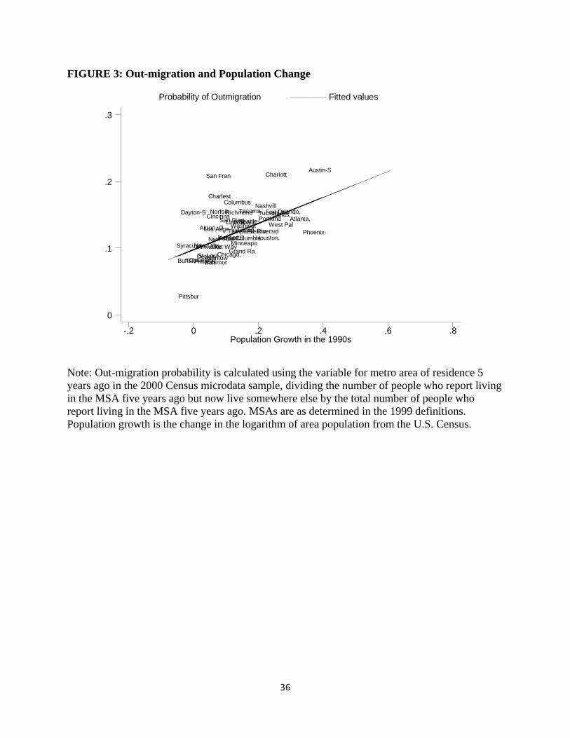
In Figure 3, we show the correlation between metropolitan area population change between 1990

and 2000 and the out-migration rate in the area between 1995 and 2000. Population change is

defined as the difference in the logarithm of population between the two census years. The out-

migration rate is defined as the share of the population that lived in the area in 1995 and that has

moved somewhere else by 2000. In some cases, we have people who are coded as living in

different regions, but who claim not to have changed houses. We assume that those people did

not actually change region over the time period.

  18

The figure shows a strongly significant 54 percent correlation. Places that are gaining population

also have the highest out-migration rate. The right view of urban growth is not that declining

places disproportionately lose people. Growing places lose people even more rapidly. The

difference between growing and declining places is that there are far fewer people coming into

declining areas.

The strong positive relationship between growth and emigration rates suggests that policies that

target declining areas are not targeting the areas with the highest levels of emigration. It also

suggests that declining places are not caught in a bad equilibrium where high expected out-

migration rates then create less investment in social capital. If anything, we would expect the

high out-migration rates to reduce social capital investment in high growth areas. Of course, if

we think that out-migration is particularly costly in declining areas, then it may still make sense

to target policies towards those areas that are in decline.

In our next figure, we turn to the overall relationship between decline and different forms of

capital investment. Figure 4 shows the well-known positive correlation between years of

schooling in 1970 and population growth between 1970 and 2000 among metropolitan areas with

more than 250,000 people in 1970. Skilled places have seen increases in population, income,

and housing prices relative to less skilled places over the last 30 years.

Skilled places have also generally become more skilled (Berry and Glaeser, 2005). Figure 5

shows the connection between the share of the population that has a college degree in 1970 and

the growth in that share between 1970 and 2000. As the share in the population with college

degrees in 1970 increases by 10 percentage points, the growth increases by 6 percentage points.

There is not only a connection between human capital and area population growth, but an

increasing tendency of high human capital people to move to high human capital places.

By contrast, the connection between area level social capital and growth is far less clear. We use

the General Social Survey (GSS), which contains survey data for years between 1972 and 2002,

to provide data on social capital. Our primary measure is group membership, which counts the

number of types of groups in which an individual is a member. This measure is quite standard in

the social capital literature (e.g. Glaeser, Sacerdote and Laibson, 2002), but its popularity owes

more to ease of use than any sort of inherent perfection. The measure does not include the

  19

intensity of engagement, and fails to account for multiple memberships within a single category

of groups (e.g. hobby groups). However, it is widely available and correlates well with other

measures of social capital.

Figure 6 shows the 4.5 percent correlation between area level group membership and population

growth between 1970 and 2000, among metropolitan areas with more than 200 respondents in

the General Social Survey. There is essentially no correlation between social capital and growth

across metropolitan areas.

Our model emphasized the link between out-migration and social capital, where higher

propensities of leaving a place were associated with less investment in area-specific groups.

Figure 7 shows the correlation between group members and out-migration across metropolitan

areas. In this case, there is a 16 percent correlation. Contrary to the model’s suggestion, places

with more out-migration have slightly more social capital, but the effect is quite weak.

Figure 8 repeats Figure 6 but uses per capita income growth at the metropolitan level as our

measure of success. Per capita income growth will include both the increasing prosperity of

people in an area and the tendency of better paid people to move into the area. Both of these

changes can be seen as a type of success. In this case, there is a -4 percent correlation between

social capital and urban success.

Figures 6 and 8 suggest that social capital is not strongly associated with area growth. Social

capital may indeed create significant positive spillovers, and nothing we have shown contradicts

that view. However, the data does not seem to support the hypothesis that areas get locked into a

bad equilibrium where expected decline creates low levels of social capital investment, which

then in turn make that expected decline a reality. We now turn to individual level data on the

connection between geographic mobility, area decline, and social capital investment.

Social Capital, Geographic Mobility, and Urban Decline

We now turn to the link between mobility and social capital investment. At the individual level,

there is a tight link between length of time in a community and different forms of social capital.

Figure 9 shows the connection between years in a place and membership in organizations.

People who have lived in a place for a long time have, perhaps unsurprisingly, more group

  20

memberships than people who are new to a place. Figure 10 shows the connection between

years in a place and voting in the last election. We only have mobility data for a few years in the

1980s, so we have shown results for the 1984 election. Again, we have a significant positive

correlation between years in a community and political engagement. DiPasquale and Glaeser

(1999) show this relationship for a broader range of social capital variables, and estimate that

about one-half of the relationship between homeownership and social capital can be linked to

reduced geographic mobility of home owners.

However, this represents a backward-looking, rather than forward-looking, relationship between

mobility and social capital investment. The model, after all, emphasized that people who expect

to move will also be less likely to invest in social capital. We test this hypothesis by looking at

individual level data from the General Social Survey and regressing social capital outcomes on

area level out-migration rates and the population growth in the metropolitan area between 1970

and 1990. Because urban decline may be different than growth, we allow for a spline in the

urban growth variable so that the slope can be different for the most slowly growing quarter of

metropolitan areas.

We will use a series of social capital variables, including number of organization memberships,

voting in local elections, and self-reported answers to questions about working to solve local

problems. Our basic regression takes the form:

(5) Social Capital = Individual Characteristics + b*Area Growth + c*Out-Migration Rate

Our individual characteristics include age, race, income and, education. The GSS income

variables are somewhat problematic since income is only available in broad categories and some

people refuse to state their income levels. We assign people the mid-point of their reported

income range. We include those who refuse to give their income, and use a dummy variable that

takes on a value of one if the person refused to give their income. We also have a dummy

variable that takes on a value of one if the income variable was top coded.

Our core area characteristics are the out-migration rate, discussed above, and population growth

between 1970 and 1990. We restricted ourselves to this period to slightly reduce the possibility

that social capital is driving growth rather than the reverse. This is a serious concern and we will

  21

return to it later. As discussed above, we use a spline so that the slope on area growth can be

different for declining and growing cities.

Table 1 shows our results. The first regression addresses membership in organizations. This

social capital variable increases mildly with income and strongly with education. These results

are all quite standard. Both area level characteristics are statistically insignificant. There is a

weak negative relationship between the out-migration probability and group membership, of no

statistical significance. Population growth is actually weakly negatively associated with group

membership for areas in relative decline. We have run such regressions for a number of different

group memberships and similarly found no significant correlations with out-migration or area

decline. There is little here to support the view that either out-migration or urban decline is

particularly bad for social capital investment.

We next look at two regressions suggesting knowledge of local events. Regression (2) looks at

whether the respondent can name his or her congressional representative. The area level

characteristics are not significantly correlated with this variable. Regression (3) looks at whether

the respondent knows the name of the local school head. In this case, growth is negatively

associated with knowledge for declining areas, but the effect is only marginally significant.

The next three regressions look at involvement in local affairs. Regression (4) looks at whether

the respondent has lobbied a local government official. Regression (5) looks at whether the

individual has started a local group. In both cases, neither out-migration nor growth are

significantly involved with local civic engagement. In regression (6), we turn to a very vague

question about whether the individual has tried to solve local problems. In this case, area level

characteristics do predict engagement. Out-migration positively predicts working to solve local

problems and more growth reduces the probability of working to solve local problems. Both of

these results go in the opposite direction from the theory discussed above.

The final regression examines voting in local elections. Neither out-migration nor growth

predicts voting. Overall, these social capital variables do not appear to be correlated with either

out-migration or growth, at least not in the manner suggested by the model. These results cast

doubt on the idea that reducing out-migration would significantly increase investment in social

capital.

  22

One issue with these regressions is that out-migration may itself be a function of social capital

and as such is not a valid explanatory variable. There is no perfect way of handling this problem,

but one method is to look at younger respondents and control for the social capital investment of

older respondents in the sample. We divide the sample by year of birth and include only people

born after 1947 (the median year of birth) in our sample. We then use the older people in the

sample to form an area level average for each social capital variable and we control for that level

of social capital. This regression can then be seen as asking whether social capital went down

among younger people in places that were declining after 1970 or that have particularly high out-

migration rates.

Table 2 shows our results. In the first regression, we again show our findings for group

membership. There is a strong positive relationship between group membership in the previous

generation and group membership among the sample in the regressions. This fact can be

interpreted as suggesting spillovers from group membership or a positive complementarity

across people in social capital investment. Alternatively, this correlation may just reflect omitted

local characteristics that raise the returns to social capital investment in some places.

While the previous generation’s group membership is statistically significant, it does not alter the

relationship between area level characteristics and social capital. Neither out-migration nor area

decline has a significant impact on group membership. The other regressions in the table show a

similar pattern. Generally, the previous generation’s investments are positively correlated with

the younger generation’s civic engagement, but controlling for this investment does not alter the

basic lack of a relationship between area out-migration or decline and social capital.

Overall, our results do not support the view that there is strong connection between social capital

and either urban decline or out-migration. Of course, there are many reasons to be skeptical

about these findings. First, reverse causality and omitted city-level variables are real concerns

and our correlations do not imply causal relationships. Second, there is so much imprecision in

many of our estimates that it is hard to rule out negative effects of out-migration and urban

decline on social capital. Nonetheless, without further evidence it would be hard to take the view

that social capital provides a strong basis for place-based policies to support declining cities.

  23

Human Capital, Income, and Urban Change

We now turn to the human capital aspects of the model, which suggested costs of subsidizing

declining places. We will do three things here. First, we will look at whether it is indeed true

that the skill premium is higher in cities that are growing. Second, we will look at the emigration

propensities of skilled and unskilled workers. Finally, we will look at the relationship between

human capital accumulation and both out-migration and urban decline.

The model assumed that skilled people would earn more in the second, growing locale. That

assumption was the basis of the prediction that out-migration would increase the returns to

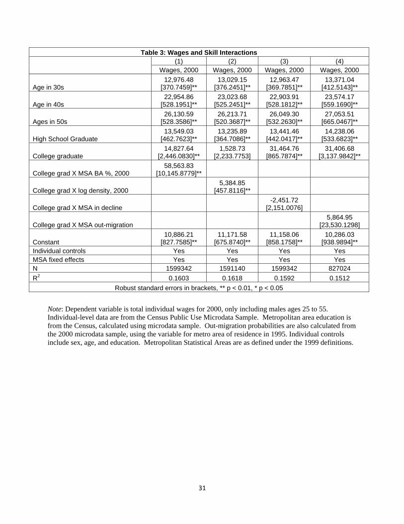
investment in skills. In Table 3, we look at wage results using the 2000 Census. To avoid issues

of labor force participation, we look only at the wages of males between 25 and 55 years of age.

Our basic regression takes the form:

(6) Income=Personal Characteristics+MSA Fixed Effects+b*BA Grad*MSA Characteristics

We control for individual characteristics, including years of schooling, and an MSA fixed effect

that takes out any impact that the metropolitan area has on the level of wages. Our interest lies in

the interaction between different metropolitan area characteristics and being a college graduate.

Do some places pay their college graduates a greater skill premium?

We attempt to answer this question in three different ways. In Table 3, we look at total wages

rather than the logarithm of wages. This is the most natural way to determine whether wages are

higher in some areas. After all, the model assumed a proportional increase in skills in the

growing areas, so this would yield a zero value for “b” if we looked at the logarithm of wages.

Since it is standard to look at the logarithm of wages, in Table 4 we also look at the logarithm of

real wages, defined as the logarithm of income divided by the American Chamber of Commerce

Research Association (ACCRA) metropolitan area price level. Since these price indices don’t

differ by education group, nominal wage results will be essentially the same as real wage results

across areas.

In the first regression of Table 3, we focus on the share of the population with college degrees as

our metropolitan area characteristic. The first regression shows that the income of people with a

college degree goes up by about 5,900 dollars as the share of the population with college degrees

  24

increases by 10 percent. This should not be interpreted as a causal link. After all, a place may

be filled with college graduates because it is a good place to be a skilled worker. Nonetheless,

the table does suggest that the returns to skills seem to be higher in some places than in others,

which in turn suggests that the prospect of out-migration may increase the returns to investing in

skill.

The second regression looks at the interaction between the logarithm of area density and having

a college degree. The returns to skill are also higher in denser areas. As density doubles, skilled

workers earn 5,400 dollars more relative to the less well-educated. This effect is quite

statistically significant. One interpretation of this fact is that density and skills are complements;

this is also supported by the propensity of high human capital industries to locate at the center of

urban areas (Glaeser and Kahn, 2001).

The third and fourth regressions look at out-migration rates and urban decline. We address urban

decline with a dummy variable that takes on a value of one if the metropolitan area is in the

bottom quartile of areas by population growth rate. In these cases, there is no significant

interaction with education. These variables may be correlated with the overall wage level in the

area, but the wages of the skilled do not seem to be particularly high or low relative to the less

skilled in places with big population changes. It therefore seems that the ability to emigrate from

declining places increases the potential returns to human capital by creating the option of moving

to denser or more skilled places, not by allowing exit from places in decline.

In Table 4, we repeat these regressions looking at the logarithm of wages. In the first regression,

we estimate a coefficient of .45 on the interaction between the share of the population with

college degrees and the individual’s own college degree. This suggests that as the share of the

population with college degrees increases by 10 percent, the wages of the skilled increase by 4.5

percent relative to the less skilled. In the second regression, we show that there is also a

significant interaction between area density and individual skills. As density doubles, the college

premium appears to rise by about 4.6 percent.

In the third regression, we find a weak negative relationship between urban decline and wages.

Areas in decline have a skill premium that is more than three percent lower than places that are

growing. In this case, the ability to leave declining areas would seem to increase the returns to

  25

skill. In the fourth regression, we find no significant relationship between out-migration rates

and the skill premium.

We now turn to out-migration probabilities, which are defined as the share of people who move

metropolitan areas between 1995 and 2000. We have calculated the out-migration rates

separately for people with more than 16 years of education (college graduates), between 12 and

16 years of education (high school graduates) and less than 12 years of education (high school

dropouts). Across the U.S. as a whole, the probability of moving across metropolitan areas rises

substantially with education. Figure 11 graphs the out-migration rates for college graduates

against the out-migration rates for high school dropouts across metropolitan areas. In almost

every area, the out-migration rate is higher for college graduates than for high school dropouts.

In many cases, the difference is enormous.

We now look at whether the propensity of different skill groups to emigrate differs with

metropolitan area growth. Figure 12 graphs the difference between college and high school out-

migration rates against population growth in the 1990s. College graduates are much more likely

to exit from declining metropolitan areas, which supports the model. Figure 13 shows that

college graduates are also disproportionately likely to flee low income areas.

These facts suggest that out-migration is a double-edged sword. On one hand, the returns to

schooling are presumably higher for people in declining areas because of the option to migrate.

On the other hand, the exodus of the skilled leaves those declining places with less human

capital. Since human capital is itself such a strong correlate of area growth, this migration may

be hurting the city’s chances for success.

Our final empirical exercise is to look at whether people become more skilled in cities where

out-migration rates are higher. Because out-migration rates and urban decline are themselves a

function of the skill level of an area, we look only at people who were between 25 and 40 years

old in the 2000 Census. We then control for the average skill level of people who were between

40 and 55 in the same year. We hope that by controlling for the skills of older people we are

minimizing the problem of reverse causality, but we still believe that these results are likely to be

somewhat compromised by those concerns. Nonetheless, Table 5 reports our results, controlling

for age and race.

  26

The first regression shows a weak positive relationship between out-migration and the share of

the population that have acquired a college degree. Urban growth is, if anything, negatively

associated with getting a college education, once we control for the skills of older people in the

city. In the second regression, we find a strong positive relationship between out-migration and

the share of the population getting a high school degree. Urban growth again predicts less skill

accumulation. This provides some weak support for the view that out-migration and skill

accumulation are positively associated, but it would be a mistake to take this too seriously.

V. Conclusion

In this paper we present a model that can justify government support for declining areas. If

people are less likely to invest in social capital when they know an area is declining, then this

creates a negative externality from decline. Subsidizing the place can work against that

externality, but it also can reduce investment in human capital if the returns to skill are higher

outside of that area. The model suggests that there are situations when it could make sense to try

to keep people committed to declining areas.

The key empirical conditions needed to justify such policies are that out-migration and decline

are strongly associated with lower levels of social capital investment. We investigate this

possibility using the General Social Survey, and find little evidence that decline is accompanied

by lower social capital; across metropolitan areas there is little connection between out-migration

and social capital investment. People who live in declining areas, or places with high out-

migration rates, are not less likely to invest in social capital. To us, this suggests that it is unwise

to believe that stemming decline will result in more place-making social capital activities.

We also look at the connection between human capital investment and urban change. We find

that growing areas do indeed offer a higher human capital premium. More skilled people are

also particularly likely to leave declining places. These facts suggest that trying to subsidize

declining places and keep people there may reduce the incentive for individuals to invest in

  27

human capital. On balance, it therefore seems unlikely to us that subsidies for declining areas are

likely to enhance social welfare.

  28

References

Austen-Smith, David and Roland Fryer (2005). “An Economic Analysis of ‘Acting White,’” Quarterly Journal of Economics, 120(2): 551-583.

Bolton, Roger (1987). "An Economic Interpretation of a `Sense of Place': Speculations and Questions." Portland, OR: meeting of Association of American Geographers and Baltimore, MD: North American meeting of Regional Science Association International.

Bolton, Roger (1992). “Place Prosperity vs People Prosperity' Revisited: An Old Issue with a New Angle.” Urban Studies Journal, 29: 185-203.

Bolton, Roger (2003). “Local Social Capital and Entrepreneurship.” with Hans Westlund, Small Business Economics, 21(2): 77-113.

DiPasquale, Denise & Edward L. Glaeser (1999). “Incentives and Social Capital: Are Homeowners Better Citizens?," Journal of Urban Economics, 45(2): 354-384.

Glaeser, Edward L. and Christoper R. Berry (2005). "The Divergence of Human Capital Levels Across Cities." NBER Working Paper #11617.

Glaeser, Edward and Joshua Gottlieb (2008). “The Economics of Place-Making Policies,” mimeographed.

Glaeser, Edward L., David Laibson and Bruce Sacerdote (2002). “An Economic Approach to Social Capital." Economic Journal, Royal Economic Society 112(483): 437-458.

Sjaastad, Larry A. (1962). "The Costs and Returns of Human Migration." The Journal of Political Economy 70(5): 80-93.

Spilimbergo, Antonio & Ubeda, Luis (2004). "A model of multiple equilibria in geographic labor mobility." Journal of Development Economics, 73(1): 107-123.

Winnick, Louis (1966). “Place Prosperity vs. People Prosperity: Welfare Considerations in the Geographic Redistribution of Economic Activity.” pp. 273-283 in Real Estate Research Program, University of California at Los Angeles, Essay in Urban Land Economics in Honor of the Sixty Fifth Birthday of Leo Grebler. Los Angeles, CA: Real Estate Research Program.

  29

TABLE 1: SOCIAL CAPITAL, OUT-MIGRATION AND GROWTH

(1) (2) (3) (4) (5) (6) (7)

Number of group

memberships Can Name U.S. Rep.

Can Name School Head

Has Lobbied local

gov't official

Has Helped start

a local group

Has Helped solve Local

problems

Usually votes in

local elections

Log(income) 0.0497** 0.0948** 0.0651 -0.00748 -0.0109 0.00393 0.0314 (0.021) (0.042) (0.044) (0.024) (0.016) (0.030) (0.025) Refused to give income 0.275 0.741* 0.475 0.0498 -0.0154 0.228 0.358 (0.20) (0.42) (0.46) (0.25) (0.18) (0.26) (0.27) Income top coded 0.719*** 0.889** 0.570 -0.0729 -0.163 0.0119 0.338 (0.21) (0.41) (0.41) (0.23) (0.16) (0.26) (0.24) Finished HS 0.667*** 0.0845 -0.0764 0.194*** 0.102** 0.137** 0.191*** (0.063) (0.087) (0.064) (0.049) (0.042) (0.051) (0.058) Has a BA 1.130*** -0.0424 0.0989 0.107*** 0.0897** 0.0812* 0.109*** (0.090) (0.050) (0.069) (0.037) (0.035) (0.043) (0.036) Out-migration Probability -0.103 0.593 -0.286 0.411 0.502 0.884** -0.689 (1.31) (1.21) (0.96) (0.40) (0.66) (0.37) (0.47) Population Growth -0.899 -0.491 -1.219* 0.0546 -0.224 -1.484*** 0.129 (below 25th percentile) (1.12) (1.26) (0.72) (0.50) (0.73) (0.41) (0.50) Population Growth 0.282 0.229 0.127 0.153 0.0246 0.135 -0.163 (above 25th percentile) (0.19) (0.21) (0.25) (0.13) (0.10) (0.090) (0.12) West -0.0837 -0.185 0.0147 -0.0606 -0.0156 0.0211 0.0212 (0.13) (0.19) (0.14) (0.076) (0.11) (0.073) (0.080) South 0.0343 0.00539 0.00664 0.00819 0.0122 0.0700 0.0238 (0.15) (0.16) (0.10) (0.056) (0.075) (0.049) (0.074) Midwest 0.227** 0.143 0.0201 0.0604 0.0206 0.0954*** 0.0877 (0.11) (0.12) (0.075) (0.036) (0.053) (0.029) (0.053) Age, Gender and Race Controls Yes Yes Yes Yes Yes Yes Yes Constant -0.0637 -0.754 -0.231 -0.474** -0.438* -0.670** -0.522* (0.28) (0.51) (0.47) (0.22) (0.23) (0.32) (0.28) Observations 6366 248 184 666 666 666 663 R-squared 0.12 0.14 0.12 0.07 0.06 0.10 0.17

Robust standard errors in parentheses, *** p<0.01, ** p<0.05, * p<0.1 Notes: Data is from the General Social Survey (GSS). Respondents were asked (1) how many types of social groups they belong to (2) to name their U.S. Representative, (3) to name the head of the local school system, (4) whether they have lobbied a local gov’t official, (5) whether they have helped start a local group, (6) whether they help solve local problems, and (7) whether they usually vote in local elections. Incomes were taken as the midpoint of intervals, and those who refused to give their income or had their income top coded were assigned a value of zero (and then assigned dummy variable values of 1 as appropriate). Out-migration probabilities for 1995-2000 were calculated using the variable for place of residence in 1995 in the 2000 Census.

  30

TABLE 2: SOCIAL CAPITAL AMONG YOUNGER RESPONDANTS

(1) (2) (3) (4) (5) (6) (7)

Number of group

memberships Can Name U.S. Rep.

Can Name School Head

Has lobbied local

gov't official

Has helped start

a local group

Has helped solve local

problems

Usually votes in

local elections

Log(income) -0.0126 0.156** 0.148* -0.00540 -0.00267 0.00443 0.0101 (0.030) (0.073) (0.080) (0.031) (0.021) (0.037) (0.035) Refused income -0.601* 0.879 1.684* -0.327 0.0538 -0.0187 -0.110 (0.32) (0.74) (0.90) (0.29) (0.26) (0.36) (0.45) Income top coded 0.0618 1.474** 1.330 -0.0195 -0.0893 -0.0221 0.203 (0.30) (0.70) (0.82) (0.28) (0.20) (0.32) (0.34) Finished HS 0.473*** -0.0196 -0.137 0.117 0.00703 0.00799 0.0933 (0.082) (0.12) (0.094) (0.075) (0.053) (0.062) (0.078) Has a BA 1.070*** -0.0149 -0.0467 0.0977** 0.107*** 0.0963** 0.125** (0.092) (0.088) (0.16) (0.046) (0.037) (0.047) (0.055) Out-migration 0.710 1.753 0.947 0.452 0.498 0.999** -0.820 Probability (1.16) (1.64) (1.95) (0.55) (0.62) (0.37) (0.64) Population Growth -1.041 -0.110 -2.731 -0.745 -0.224 -2.104*** -0.152 (below 25th percentile) (1.23) (1.31) (1.63) (0.61) (0.76) (0.59) (0.64) Population Growth 0.278 -0.0734 0.376 0.369** -0.0451 0.134 -0.276 (above 25th percentile) (0.26) (0.36) (0.45) (0.16) (0.090) (0.10) (0.17) West -0.132 -0.218 0.0395 -0.117 0.000532 0.0696 0.122 (0.16) (0.31) (0.28) (0.075) (0.093) (0.067) (0.11) South 0.0862 0.0353 -0.0206 -0.0192 0.0513 0.0769 0.0850 (0.19) (0.22) (0.24) (0.064) (0.082) (0.059) (0.10) Midwest 0.154 0.108 0.128 0.103** 0.0348 0.141*** 0.155** (0.13) (0.15) (0.15) (0.045) (0.061) (0.045) (0.073) Avg. Dependent Variable among older cohort 0.401*** 0.148 -0.0969 -0.204 0.284 -0.210* -0.338* (0.13) (0.19) (0.17) (0.14) (0.18) (0.12) (0.20) Age, Gender and Race Controls Yes Yes Yes Yes Yes Yes Yes Constant 2.837*** -1.047 0.0166 0.155 0.874 1.444** -0.723 (0.75) (1.00) (1.50) (0.62) (0.58) (0.55) (0.78) Observations 3094 114 80 400 400 400 398 R-squared 0.10 0.25 0.19 0.09 0.08 0.10 0.11

Robust standard errors in parentheses, *** p<0.01, ** p<0.05, * p<0.1 Notes: Data is from the General Social Survey (GSS). Respondents were asked (1) how many types of social groups they belong to (2) to name their U.S. Representative, (3) to name the head of the local school system, (4) whether they have lobbied a local gov’t official, (5) whether they have helped start a local group, (6) whether they help solve local problems, and (7) whether they usually vote in local elections. Incomes were taken as the midpoint of intervals, and those who refused to give their income or had their income top coded were assigned a value of zero (and then assigned dummy variable values of 1 as appropriate). Out-migration probabilities for 1995-2000 were calculated using the variable for place of residence in 1995 in the 2000 Census.

  31

Table 3: Wages and Skill Interactions (1) (2) (3) (4) Wages, 2000 Wages, 2000 Wages, 2000 Wages, 2000

Age in 30s 12,976.48

[370.7459]** 13,029.15

[376.2451]** 12,963.47

[369.7851]** 13,371.04

[412.5143]**

Age in 40s 22,954.86

[528.1951]** 23,023.68

[525.2451]** 22,903.91

[528.1812]** 23,574.17

[559.1690]**

Ages in 50s 26,130.59

[528.3586]** 26,213.71

[520.3687]** 26,049.30

[532.2630]** 27,053.51

[665.0467]**

High School Graduate 13,549.03

[462.7623]** 13,235.89

[364.7086]** 13,441.46

[442.0417]** 14,238.06

[533.6823]**

College graduate 14,827.64

[2,446.0830]** 1,528.73

[2,233.7753] 31,464.76

[865.7874]** 31,406.68

[3,137.9842]**

College grad X MSA BA %, 2000 58,563.83

[10,145.8779]**

College grad X log density, 2000 5,384.85

[457.8116]**

College grad X MSA in decline -2,451.72

[2,151.0076]

College grad X MSA out-migration 5,864.95

[23,530.1298]

Constant 10,886.21

[827.7585]** 11,171.58

[675.8740]** 11,158.06

[858.1758]** 10,286.03

[938.9894]** Individual controls Yes Yes Yes Yes MSA fixed effects Yes Yes Yes Yes N 1599342 1591140 1599342 827024 R2 0.1603 0.1618 0.1592 0.1512

Robust standard errors in brackets, ** p < 0.01, * p < 0.05

Note: Dependent variable is total individual wages for 2000, only including males ages 25 to 55. Individual-level data are from the Census Public Use Microdata Sample. Metropolitan area education is from the Census, calculated using microdata sample. Out-migration probabilities are also calculated from the 2000 microdata sample, using the variable for metro area of residence in 1995. Individual controls include sex, age, and education. Metropolitan Statistical Areas are as defined under the 1999 definitions.

  32

Note: Dependent variable is the logarithm of individual wages divided by ACCRA metro-area price indices for 2000, including only males ages 25 to 55. Individual-level data are from the Census Public Use Microdata Sample. Metropolitan area education is from the Census, calculated using microdata sample. Out-migration probabilities are also calculated from the 2000 microdata sample using the variable for metro area of residence in 1995. Individual controls include sex, age, and education. Metropolitan Statistical Areas are as defined under the 1999 definitions.

Table 4: Log of Real Wages and Skill Interactions (1) (2) (3) (4) Log real wages Log real wages Log real wages Log real wages

Age in 30s 0.2737

[0.0050]** 0.2740

[0.0049]** 0.2735

[0.0050]** 0.2742

[0.0060]**

Age in 40s 0.4266

[0.0067]** 0.4272

[0.0065]** 0.4261

[0.0068]** 0.4295

[0.0093]**

Age in 50s 0.4731

[0.0070]** 0.4739

[0.0066]** 0.4725

[0.0071]** 0.4753

[0.0100]**

High school graduate 0.4097

[0.0130]** 0.4072

[0.0119]** 0.4085

[0.0128]** 0.4313

[0.0155]**

College graduate 0.3460

[0.0249]** 0.2187

[0.0206]** 0.4751

[0.0091]** 0.4452

[0.0317]**

College grad X MSA BA %, 2000 0.4488

[0.0919]**

College grad X log density 2000 0.0458

[0.0039]**

College grad X MSA in decline -0.0332 [0.0222]

College grad X MSA outmigration 0.3106 [0.2270]

Constant 8.4119

[0.0139]** 8.4139

[0.0122]** 8.4143

[0.0138]** 8.3687

[0.0158]** MSA fixed effects Yes Yes Yes Yes N 1296185 1294419 1296185 767962 R2 0.2726 0.2733 0.2724 0.3065

Robust standard errors in brackets, ** p < 0.01, * p < 0.05

  33

TABLE 5: Education and Out-Migration

(1) (2) Has a BA Finished HS Age -0.00196*** 0.0000897 (0.00055) (0.00036) Male -0.0184*** -0.0288*** (0.0025) (0.0017) Black -0.184*** -0.0594*** (0.011) (0.011) Asian 0.151*** 0.00820 (0.019) (0.017) Other Race -0.223*** -0.267*** (0.011) (0.011) % of those 40-55 in the MSA with a BA 1.003*** (0.053) Out-migration Probability 0.168 0.330*** (0.13) (0.060) Population Growth (below 25th percentile) -0.203 -0.184** (0.15) (0.087) Population Growth (above 25th percentile) -0.0594*** -0.0524*** (0.015) (0.011) % of those 40-55 in the MSA that finished HS 0.667*** (0.049) Constant 0.111*** 0.299*** (0.027) (0.051) Observations 329561 329561 R-squared 0.08 0.08

Robust standard errors in parentheses, *** p<0.01, ** p<0.05, * p<0.1

Note: Dependent variables are binary indicators for highest educational attainment. Only people ages 25 to 40 are included. Individual-level data are from the 2000 Census Public Use Microdata Sample. Metropolitan area education is from the Census, also calculated using microdata sample. Outmigration probabilities also calculated from the 2000 microdata sample using the variable for metro area of residence in 1995. Metropolitan Statistical Areas are as defined under the 1999 definitions.

  34

FIGURE 1: Happiness and Urban Growth in the 1990s

Population Growth in the 1990s

Percent happy in MSA .

-.2 0 .2 .4 .6

.8

.85

.9

.95

AllentowAtlanta,

Baltimor

Buffalo-

Charlest

Charlott

Chicago,

Clevelan

Columbus

Dallas,

Detroit,

Fort Way

Fresno,

Houston,

IndianapKansas C

Knoxvill

Los Ange

Minneapo

Nashvill

New Orle

New York

Norfolk-

Philadel

Phoenix-

Pittsbur

PortlandRichmond

Riversid

St. Loui

San Dieg

San Fran

Seattle-Tacoma,

Tampa-St

Washingt

Note: Happiness refers to the share of population reporting being somewhat or very happy in the General Social Survey between 1972 and 2002. Population growth is the change in the logarithm of area population from the U.S. Census.

 

 

 

 

 

 

 

 

 

 

 

  35

FIGURE 2: Multiple Equilibria and Social Capital

0

0.2

0.4

0.6

0.8

1

1.2

0 0.1 0.2 0.3 0.4 0.5 0.6 0.7 0.8 0.9 1

Share Investing in Social Capital

Cost of Investing

Returns to SocialCapitalOut-Migration Rate

Note: Figure is a numerical example of a model described in the text.

  36

FIGURE 3: Out-migration and Population Change

Population Growth in the 1990s

Probability of Outmigration Fitted values

-.2 0 .2 .4 .6 .8

0

.1

.2

.3

Buffalo-

Syracuse

Knoxvill

Clevelan

Richmond

New YorkTampa-St

AllentowDetroit,

Columbia

Baltimor

CincinnaWashingt

CharlottAustin-S

Portland

Phoenix-

Minneapo

Philadel

Pittsbur

Grand Ra

Atlanta,

Jackson,

Chicago,

RiversidIndianap

Charlest

Norfolk-

Houston,

Fort LauDallas, San DiegLittle R

New Orle

Akron, O

Nashvill

Fort Way

Fresno, West Pal

Los Ange

Tucson, Orlando,Tacoma, Dayton-S

Milwauke

Seattle-

Kansas C

St. Loui

Columbus

San Fran

 

Note: Out-migration probability is calculated using the variable for metro area of residence 5 years ago in the 2000 Census microdata sample, dividing the number of people who report living in the MSA five years ago but now live somewhere else by the total number of people who report living in the MSA five years ago. MSAs are as determined in the 1999 definitions. Population growth is the change in the logarithm of area population from the U.S. Census.

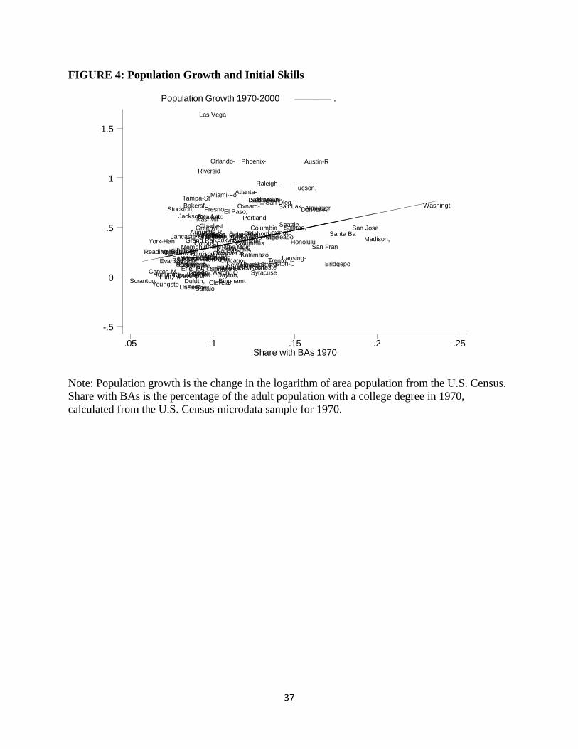
  37

FIGURE 4: Population Growth and Initial Skills

Share with BAs 1970

Population Growth 1970-2000 .

.05 .1 .15 .2 .25

-.5

0

.5

1

1.5

Akron, OAlbany-S

Albuquer

Allentow

Atlanta-

Augusta-

Austin-R

Bakersfi

Baltimor

Baton Ro

Beaumont

Binghamt

Birmingh

Boston-C Bridgepo

Buffalo-

Canton-MCharlest

CharlestCharlott

Chattano

Chicago-Cincinna

Clevelan

Columbia

Columbus

ColumbusCorpus C

Dallas-F

Davenpor Dayton,

Denver-A

Des Moin

Detroit-Duluth,

El Paso,

Erie, PAEvansvil

Flint, M

Fort Way

Fresno,

Grand RaGreensboGreenvil

Harrisbu

Hartford

Honolulu

Houston-

Huntingt

Indianap

Jackson,

Jacksonv

KalamazoKansas C

KnoxvillLancaste

Lansing-

Las Vega

LexingtoLittle RLos Ange

Louisvil

Madison,Memphis,

Miami-Fo

Milwauke

Minneapo

Mobile,

Nashvill

New HaveNew Orle

New York

Oklahoma

Omaha-Co

Orlando-

Oxnard-T

Peoria, Philadel

Phoenix-

Pittsbur

Portland

Portland

Poughkee

Providen

Raleigh-

Reading,

Richmond

Riversid

RochesteRockford

Sacramen

St. Loui

Salinas,

Salt LakSan Anto

San Dieg

San Fran

San JoseSanta Ba

Scranton

Seattle-

ShrevepoSouth Be

Spokane,

Springfi

Stockton

Syracuse

Tampa-St

Toledo,

Trenton-

Tucson,

Tulsa, O

Utica-Ro

Virginia

Washingt

Wichita,

Winston-

Worceste

York-Han

Youngsto

 

Note: Population growth is the change in the logarithm of area population from the U.S. Census. Share with BAs is the percentage of the adult population with a college degree in 1970, calculated from the U.S. Census microdata sample for 1970.

 

 

 

 

 

 

 

 

 

 

  38

FIGURE 5: Initial Education Level and Growth in Education 

Share with BAs 1970

Change in Share with BAs 1970-2 .

.05 .1 .15 .2 .25

.05

.1

.15

.2

.25

Akron, O

Albany-S

Albuquer

Allentow

Atlanta-

Augusta-

Austin-R

Bakersfi

Baltimor

Baton Ro

Beaumont

Binghamt

Birmingh

Boston-CBridgepo

Buffalo-

Canton-M

Charlest

Charlest

Charlott

Chattano

Chicago-

Cincinna

Clevelan Columbia

Columbus

Columbus

Corpus C

Dallas-F

DavenporDayton,

Denver-A

Des Moin

Detroit-

Duluth,

El Paso,

Erie, PA

Evansvil

Flint, M

Fort Way

Fresno,

Grand RaGreensboGreenvil

Harrisbu

Hartford

HonoluluHouston-

Huntingt

Indianap

Jackson,JacksonvKalamazo

Kansas C

Knoxvill

Lancaste

Lansing-

Las Vega

Lexingto

Little R

Los AngeLouisvil

Madison,

Memphis, Miami-Fo

Milwauke

Minneapo

Mobile,

Nashvill New Have

New Orle

New York

Oklahoma

Omaha-Co

Orlando-Oxnard-T

Peoria,

Philadel

Phoenix-

Pittsbur

Portland

Portland

Poughkee

Providen

Raleigh-

Reading,

Richmond

Riversid

Rocheste

Rockford

Sacramen

St. Loui

Salinas,

Salt LakSan Anto

San Dieg

San Fran

San Jose

Santa BaScranton

Seattle-

Shrevepo

South BeSpokane,

Springfi

Stockton

SyracuseTampa-St

Toledo,

Trenton-

Tucson, Tulsa, O

Utica-Ro

Virginia

Washingt

Wichita,

Winston-

Worceste

York-Han

Youngsto

 

Note: Change in share with BAs is the share of the adult population in the MSA with a BA in 2000 minus the share of the adult population in the MSA with a BA in 1970. Share with BAs in 1970 is the share of the adult population in the MSA with a BA in 1970. Both variables are calculated from the Census microdata samples (for 1970 and 2000).

 

 

 

 

 

 

 

 

 

 

  39

FIGURE 6: Group Membership and Population Growth

Population Growth 1970-2000

Group Membership .

0 1 2

1.5

2

2.5

Allentow

Atlanta,

Baltimor

Buffalo-

Charlest

CharlottChicago,

Clevelan

Columbus

Dallas,

Detroit,

Fort Way

Fresno,

Houston,

Indianap

Kansas CKnoxvill

Los Ange

Minneapo

Nashvill

New OrleNew York

Norfolk-

Philadel

Phoenix-

Pittsbur

Portland

Richmond

Riversid

St. Loui

San Dieg

San Fran

Seattle-

Tacoma,

Tampa-St

Washingt

 

Note: Group membership is the average number of types of social groups a person in the MSA belongs to, calculated from the GSS. Population growth is the change in the logarithm of area population from the U.S. Census.

 

 

 

 

 

 

 

 

 

 

 

  40

FIGURE 7: Group Membership and Out-migration

Probability of Outmigration

Group Membership Fitted values

0 .1 .2

0

1

2

3

4

Gary

Buffalo-

Syracuse

Knoxvill

Clevelan

RichmondNew YorkTampa-St

Allentow

Detroit,ColumbiaBaltimor

CincinnaWashingt

Charlott

Austin-S

PortlandPhoenix-Minneapo

Philadel

Pittsbur

Grand RaAtlanta,

Jackson,

Chicago,

Riversid

Indianap CharlestNorfolk-

Houston,

Fort Lau

Dallas, San DiegLittle R

New Orle

Akron, O

NashvillFort Way

Fresno,

West Pal

Los Ange

Tucson,

Orlando,

Tacoma, Dayton-S

Milwauke

Seattle-

Kansas C

St. LouiColumbus

San Fran

 

Note: Group membership is the average number of types of social groups a person in the MSA belongs to, calculated from the GSS. Out-migration probability is calculated using the variable for metro area of residence 5 years ago in the 2000 Census microdata sample, dividing the number of people who report living in the MSA five years ago but now live somewhere else by the total number of people who report living in the MSA five years ago.

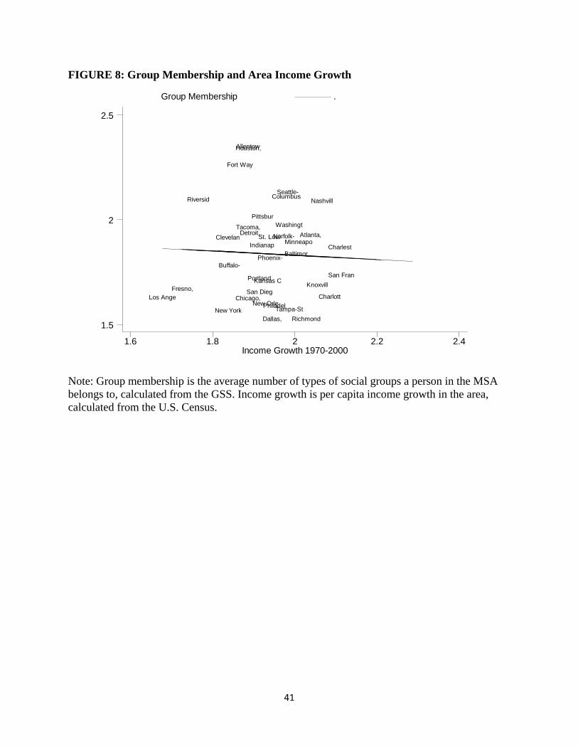
  41

FIGURE 8: Group Membership and Area Income Growth

Income Growth 1970-2000

Group Membership .

1.6 1.8 2 2.2 2.4

1.5

2

2.5

Allentow

Atlanta,

Baltimor

Buffalo-

Charlest

CharlottChicago,

Clevelan

Columbus

Dallas,

Detroit,

Fort Way

Fresno,

Houston,

Indianap

Kansas C Knoxvill

Los Ange

Minneapo

Nashvill

New OrleNew York

Norfolk-

Philadel

Phoenix-

Pittsbur

Portland

Richmond

Riversid

St. Loui

San Dieg

San Fran

Seattle-

Tacoma,

Tampa-St

Washingt

 

Note: Group membership is the average number of types of social groups a person in the MSA belongs to, calculated from the GSS. Income growth is per capita income growth in the area, calculated from the U.S. Census.

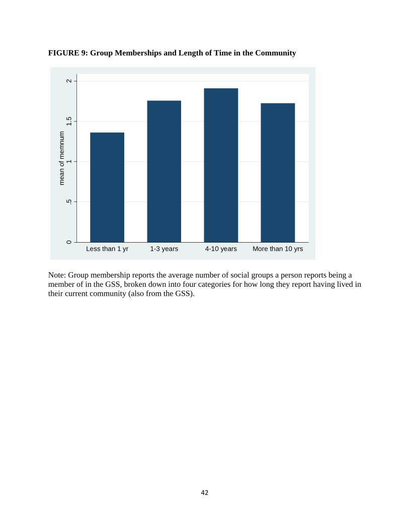
  42

FIGURE 9: Group Memberships and Length of Time in the Community

0.5

11.

52

mea

n of

mem

num

Less than 1 yr 1-3 years 4-10 years More than 10 yrs 

Note: Group membership reports the average number of social groups a person reports being a member of in the GSS, broken down into four categories for how long they report having lived in their current community (also from the GSS).

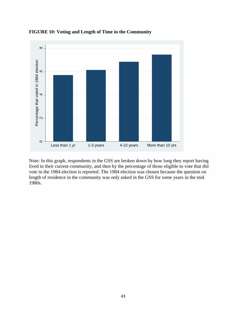
  43

FIGURE 10: Voting and Length of Time in the Community

0.2

.4.6

.8P

erce

ntag

e th

at v

oted

in 1

984

elec

tion

Less than 1 yr 1-3 years 4-10 years More than 10 yrs 

Note: In this graph, respondents in the GSS are broken down by how long they report having lived in their current community, and then by the percentage of those eligible to vote that did vote in the 1984 election is reported. The 1984 election was chosen because the question on length of residence in the community was only asked in the GSS for some years in the mid 1980s.

  44

FIGURE 11: College Graduate vs. HS Dropout Outmigration Probabilities

HS Dropout's Outmigration Prob.

College Graduate's Outmigration Fitted values

0 .1 .2

.05

.1

.15

.2

.25

Sarasota

Salt Lak

Canton-M

Albuquer

McAllen-

Youngsto

San Jose

Sacramen

Toledo,

Scranton

Modesto,

Wichita,

Baton Ro

Melbourn

Lancaste

Louisvil

Bakersfi

Lakeland

San Anto

Pensacol

StocktonSpokane,

Las Vega

Boise Ci

Harrisbu

Greensbo

MonmouthBuffalo-

Syracuse

Knoxvill

Clevelan

Richmond

New YorkTampa-St

AllentowDetroit,

Columbia

Baltimor

Cincinna

Washingt

Charlott

Austin-S

Portland

Phoenix-Minneapo

Philadel

Pittsbur

Grand Ra

Atlanta,Jackson,

Chicago,

Riversid

Indianap

Charlest

Norfolk-

Houston,

Fort LauDallas,

San Dieg

Little R

New Orle

Akron, O

Nashvill

Fort Way

Fresno,

West PalLos Ange

Tucson,

Orlando,

Tacoma,

Dayton-S

Milwauke Seattle-

Kansas CSt. Loui

Columbus

San Fran

 

Note: This figure graphs an area’s out-migration probability for its college graduates vs. its out-migration probability for its high school dropouts. A person’s level of education is determined from the U.S. Census microdata sample (we classify those who complete less than 12 years of schooling as high school dropouts), and out-migration probabilities are also calculated using geographic and migration variables in the Census microdata sample.

 

 

 

 

 

 

 

 

 

 

  45

FIGURE 12: Difference in BA and HS Migration Rates and Population Growth

Population Growth in the 1990s

BA Migration-HS Migration Fitted values

-.2 0 .2 .4 .6

0

.05

.1

Sarasota

Salt Lak

Canton-M

Albuquer

McAllen-

Youngsto

San Jose

Sacramen

Toledo,

Scranton

Modesto,

Wichita,

Baton Ro

Melbourn

Lancaste

Louisvil

Bakersfi

Lakeland

San Anto

Pensacol

StocktonSpokane,

Las VegaBoise Ci

Harrisbu

Greensbo

Monmouth

Buffalo-

SyracuseKnoxvill

Clevelan

RichmondNew York

Tampa-St

AllentowDetroit,

Columbia

Baltimor

Cincinna

Washingt

Charlott

Austin-S

Portland

Phoenix-

Minneapo

Philadel

Pittsbur

Grand RaAtlanta,

Jackson,

Chicago,

Riversid

Indianap

Charlest

Norfolk-

Houston,Fort Lau

Dallas,

San Dieg

Little RNew Orle

Akron, O

Nashvill

Fort WayFresno,

West PalLos Ange

Tucson,

Orlando,

Tacoma,

Dayton-S

Milwauke

Seattle-

Kansas C

St. Loui Columbus

San Fran

 

Note: This figure plots the difference in outmigration probabilities between those who finish college and those who finish high school against an area’s population growth in the 1990s. Population growth is calculated as the change in the logarithm of an area’s population between 2000 and 1990. Both variables are calculated using the Census microdata sample.

  46

FIGURE 13: Difference in BA and HS Migration Rates and Income

 

Income per Capita, 1990

BA Migration-HS Migration Fitted values

5000 10000 15000 20000 25000

0

.05

.1

Sarasota

Salt Lak

Canton-M

Albuquer

McAllen-

Youngsto

San Jose

Sacramen

Toledo,

Scranton

Modesto,

Wichita,

Baton Ro

Melbourn

Lancaste

Louisvil

Bakersfi

Lakeland

San Anto

Pensacol

StocktonSpokane,

Las VegaBoise Ci

Harrisbu

Greensbo

Monmouth

Buffalo-

SyracuseKnoxvill

Clevelan

RichmondNew York

Tampa-St

AllentowDetroit,

Columbia

Baltimor

Cincinna

Washingt

Charlott

Austin-S

Portland

Phoenix-

Minneapo

Philadel

Pittsbur

Grand RaAtlanta,

Jackson,

Chicago,

Riversid

Indianap

Charlest

Norfolk-

Houston,Fort Lau

Dallas,

San Dieg

Little RNew Orle

Akron, O

Nashvill

Fort WayFresno,

West PalLos Ange

Tucson,

Orlando,

Tacoma,

Dayton-S

Milwauke

Seattle-

Kansas C

St. LouiColumbus

San Fran

 

Note: This figure plots the difference in outmigration probabilities between those who finish college and those who finish high school against an area’s income per capita in 1990. Both the outmigration proabilities and income per capita are calculated using the U.S. Census.