soc500: applied social statistics week 1: introduction … · soc500: applied social statistics...
TRANSCRIPT

Soc500: Applied Social Statistics
Week 1: Introduction and Probability
Brandon Stewart1
Princeton
September 14, 2016
1These slides are heavily influenced by Matt Blackwell, Adam Glynn and Matt Salganik.The spam filter segment is adapted from Justin Grimmer and Dan Jurafsky. Illustrations byShay O’Brien.
Stewart (Princeton) Week 1: Introduction and Probability September 14, 2016 1 / 62

Where We’ve Been and Where We’re Going...
Last WeekI methods campI pre-grad school life
This WeekI Wednesday
F welcomeF basics of probability
Next WeekI random variablesI joint distributions
Long RunI probability → inference → regression
Questions?
Stewart (Princeton) Week 1: Introduction and Probability September 14, 2016 2 / 62

Welcome and Introductions
Soc500: Applied Social Statistics
II . . . am an Assistant Professor in Sociology.I . . . am trained in political science and statisticsI . . . do research in methods and statistical text analysisI . . . love doing collaborative researchI . . . talk very quickly
Your PreceptorsI sage guides of all thingsI Ian LundbergI Simone Zhang
Stewart (Princeton) Week 1: Introduction and Probability September 14, 2016 3 / 62

Welcome and Introductions
Soc500: Applied Social Statistics
I
I . . . am an Assistant Professor in Sociology.I . . . am trained in political science and statisticsI . . . do research in methods and statistical text analysisI . . . love doing collaborative researchI . . . talk very quickly
Your PreceptorsI sage guides of all thingsI Ian LundbergI Simone Zhang
Stewart (Princeton) Week 1: Introduction and Probability September 14, 2016 3 / 62

Welcome and Introductions
Soc500: Applied Social Statistics
II . . . am an Assistant Professor in Sociology.
I . . . am trained in political science and statisticsI . . . do research in methods and statistical text analysisI . . . love doing collaborative researchI . . . talk very quickly
Your PreceptorsI sage guides of all thingsI Ian LundbergI Simone Zhang
Stewart (Princeton) Week 1: Introduction and Probability September 14, 2016 3 / 62

Welcome and Introductions
Soc500: Applied Social Statistics
II . . . am an Assistant Professor in Sociology.I . . . am trained in political science and statistics
I . . . do research in methods and statistical text analysisI . . . love doing collaborative researchI . . . talk very quickly
Your PreceptorsI sage guides of all thingsI Ian LundbergI Simone Zhang
Stewart (Princeton) Week 1: Introduction and Probability September 14, 2016 3 / 62

Welcome and Introductions
Soc500: Applied Social Statistics
II . . . am an Assistant Professor in Sociology.I . . . am trained in political science and statisticsI . . . do research in methods and statistical text analysis
I . . . love doing collaborative researchI . . . talk very quickly
Your PreceptorsI sage guides of all thingsI Ian LundbergI Simone Zhang
Stewart (Princeton) Week 1: Introduction and Probability September 14, 2016 3 / 62

Welcome and Introductions
Soc500: Applied Social Statistics
II . . . am an Assistant Professor in Sociology.I . . . am trained in political science and statisticsI . . . do research in methods and statistical text analysisI . . . love doing collaborative research
I . . . talk very quickly
Your PreceptorsI sage guides of all thingsI Ian LundbergI Simone Zhang
Stewart (Princeton) Week 1: Introduction and Probability September 14, 2016 3 / 62

Welcome and Introductions
Soc500: Applied Social Statistics
II . . . am an Assistant Professor in Sociology.I . . . am trained in political science and statisticsI . . . do research in methods and statistical text analysisI . . . love doing collaborative researchI . . . talk very quickly
Your PreceptorsI sage guides of all thingsI Ian LundbergI Simone Zhang
Stewart (Princeton) Week 1: Introduction and Probability September 14, 2016 3 / 62

Welcome and Introductions
Soc500: Applied Social Statistics
II . . . am an Assistant Professor in Sociology.I . . . am trained in political science and statisticsI . . . do research in methods and statistical text analysisI . . . love doing collaborative researchI . . . talk very quickly
Your Preceptors
I sage guides of all thingsI Ian LundbergI Simone Zhang
Stewart (Princeton) Week 1: Introduction and Probability September 14, 2016 3 / 62

Welcome and Introductions
Soc500: Applied Social Statistics
II . . . am an Assistant Professor in Sociology.I . . . am trained in political science and statisticsI . . . do research in methods and statistical text analysisI . . . love doing collaborative researchI . . . talk very quickly
Your PreceptorsI sage guides of all things
I Ian LundbergI Simone Zhang
Stewart (Princeton) Week 1: Introduction and Probability September 14, 2016 3 / 62

Welcome and Introductions
Soc500: Applied Social Statistics
II . . . am an Assistant Professor in Sociology.I . . . am trained in political science and statisticsI . . . do research in methods and statistical text analysisI . . . love doing collaborative researchI . . . talk very quickly
Your PreceptorsI sage guides of all thingsI Ian Lundberg
I Simone Zhang
Stewart (Princeton) Week 1: Introduction and Probability September 14, 2016 3 / 62

Welcome and Introductions
Soc500: Applied Social Statistics
II . . . am an Assistant Professor in Sociology.I . . . am trained in political science and statisticsI . . . do research in methods and statistical text analysisI . . . love doing collaborative researchI . . . talk very quickly
Your PreceptorsI sage guides of all thingsI Ian LundbergI Simone Zhang
Stewart (Princeton) Week 1: Introduction and Probability September 14, 2016 3 / 62
1 Welcome
2 Goals
3 Ways to Learn
4 Structure of Course
5 Introduction to ProbabilityWhat is Probability?Sample Spaces and EventsProbability FunctionsMarginal, Joint and Conditional ProbabilityBayes’ RuleIndependence
6 Fun With History
Stewart (Princeton) Week 1: Introduction and Probability September 14, 2016 4 / 62

The Core Strategy
Goal: get you ready to quantitative work
First in a two course sequence replication project(for graduate students, part of a longer arc)
Difficult course but with many resources to support you.
When we are done you will be able to teach yourself many things
Stewart (Princeton) Week 1: Introduction and Probability September 14, 2016 5 / 62
The Core Strategy
Goal: get you ready to quantitative work
First in a two course sequence replication project
(for graduate students, part of a longer arc)
Difficult course but with many resources to support you.
When we are done you will be able to teach yourself many things
Stewart (Princeton) Week 1: Introduction and Probability September 14, 2016 5 / 62

The Core Strategy
Goal: get you ready to quantitative work
First in a two course sequence replication project(for graduate students, part of a longer arc)
Difficult course but with many resources to support you.
When we are done you will be able to teach yourself many things
Stewart (Princeton) Week 1: Introduction and Probability September 14, 2016 5 / 62

Specific Goals
For the semesterI critically read, interpret and replicate the quantitative content
of many articles in the quantitative social sciencesI conduct, interpret, and communicate results from analysis using
multiple regressionI explain the limitations of observational data for making causal
claimsI write clean, reusable, and reliable R code.I feel empowered working with data
Stewart (Princeton) Week 1: Introduction and Probability September 14, 2016 6 / 62

Specific Goals
For the semester
I critically read, interpret and replicate the quantitative contentof many articles in the quantitative social sciences
I conduct, interpret, and communicate results from analysis usingmultiple regression
I explain the limitations of observational data for making causalclaims
I write clean, reusable, and reliable R code.I feel empowered working with data
Stewart (Princeton) Week 1: Introduction and Probability September 14, 2016 6 / 62

Specific Goals
For the semesterI critically read, interpret and replicate the quantitative content
of many articles in the quantitative social sciences
I conduct, interpret, and communicate results from analysis usingmultiple regression
I explain the limitations of observational data for making causalclaims
I write clean, reusable, and reliable R code.I feel empowered working with data
Stewart (Princeton) Week 1: Introduction and Probability September 14, 2016 6 / 62

Specific Goals
For the semesterI critically read, interpret and replicate the quantitative content
of many articles in the quantitative social sciencesI conduct, interpret, and communicate results from analysis using
multiple regression
I explain the limitations of observational data for making causalclaims
I write clean, reusable, and reliable R code.I feel empowered working with data
Stewart (Princeton) Week 1: Introduction and Probability September 14, 2016 6 / 62

Specific Goals
For the semesterI critically read, interpret and replicate the quantitative content
of many articles in the quantitative social sciencesI conduct, interpret, and communicate results from analysis using
multiple regressionI explain the limitations of observational data for making causal
claims
I write clean, reusable, and reliable R code.I feel empowered working with data
Stewart (Princeton) Week 1: Introduction and Probability September 14, 2016 6 / 62

Specific Goals
For the semesterI critically read, interpret and replicate the quantitative content
of many articles in the quantitative social sciencesI conduct, interpret, and communicate results from analysis using
multiple regressionI explain the limitations of observational data for making causal
claimsI write clean, reusable, and reliable R code.
I feel empowered working with data
Stewart (Princeton) Week 1: Introduction and Probability September 14, 2016 6 / 62

Specific Goals
For the semesterI critically read, interpret and replicate the quantitative content
of many articles in the quantitative social sciencesI conduct, interpret, and communicate results from analysis using
multiple regressionI explain the limitations of observational data for making causal
claimsI write clean, reusable, and reliable R code.I feel empowered working with data
Stewart (Princeton) Week 1: Introduction and Probability September 14, 2016 6 / 62

Specific Goals
For the yearI conduct, interpret, and communicate results from analysis using
generalized linear modelsI understand the fundamental ideas of missing data, modern
causal inference, and hierarchical modelsI build a solid, reproducible research pipeline to go from raw data
to final paperI provide you with the tools to produce your own research (e.g.
second year empirical paper).
Stewart (Princeton) Week 1: Introduction and Probability September 14, 2016 7 / 62

Specific Goals
For the year
I conduct, interpret, and communicate results from analysis usinggeneralized linear models
I understand the fundamental ideas of missing data, moderncausal inference, and hierarchical models
I build a solid, reproducible research pipeline to go from raw datato final paper
I provide you with the tools to produce your own research (e.g.second year empirical paper).
Stewart (Princeton) Week 1: Introduction and Probability September 14, 2016 7 / 62
Specific Goals
For the yearI conduct, interpret, and communicate results from analysis using
generalized linear models
I understand the fundamental ideas of missing data, moderncausal inference, and hierarchical models
I build a solid, reproducible research pipeline to go from raw datato final paper
I provide you with the tools to produce your own research (e.g.second year empirical paper).
Stewart (Princeton) Week 1: Introduction and Probability September 14, 2016 7 / 62

Specific Goals
For the yearI conduct, interpret, and communicate results from analysis using
generalized linear modelsI understand the fundamental ideas of missing data, modern
causal inference, and hierarchical models
I build a solid, reproducible research pipeline to go from raw datato final paper
I provide you with the tools to produce your own research (e.g.second year empirical paper).
Stewart (Princeton) Week 1: Introduction and Probability September 14, 2016 7 / 62

Specific Goals
For the yearI conduct, interpret, and communicate results from analysis using
generalized linear modelsI understand the fundamental ideas of missing data, modern
causal inference, and hierarchical modelsI build a solid, reproducible research pipeline to go from raw data
to final paper
I provide you with the tools to produce your own research (e.g.second year empirical paper).
Stewart (Princeton) Week 1: Introduction and Probability September 14, 2016 7 / 62

Specific Goals
For the yearI conduct, interpret, and communicate results from analysis using
generalized linear modelsI understand the fundamental ideas of missing data, modern
causal inference, and hierarchical modelsI build a solid, reproducible research pipeline to go from raw data
to final paperI provide you with the tools to produce your own research (e.g.
second year empirical paper).
Stewart (Princeton) Week 1: Introduction and Probability September 14, 2016 7 / 62

Why R?
It’s free
It’s extremely powerful, but relatively simple to do basic stats
It’s the de facto standard in many applied statistical fieldsI great community supportI continuing developmentI massive number of supporting packages
It will help you do research
Stewart (Princeton) Week 1: Introduction and Probability September 14, 2016 8 / 62

Why R?
It’s free
It’s extremely powerful, but relatively simple to do basic stats
It’s the de facto standard in many applied statistical fields
I great community supportI continuing developmentI massive number of supporting packages
It will help you do research
Stewart (Princeton) Week 1: Introduction and Probability September 14, 2016 8 / 62

Why R?
It’s free
It’s extremely powerful, but relatively simple to do basic stats
It’s the de facto standard in many applied statistical fieldsI great community support
I continuing developmentI massive number of supporting packages
It will help you do research
Stewart (Princeton) Week 1: Introduction and Probability September 14, 2016 8 / 62
Why R?
It’s free
It’s extremely powerful, but relatively simple to do basic stats
It’s the de facto standard in many applied statistical fieldsI great community supportI continuing development
I massive number of supporting packages
It will help you do research
Stewart (Princeton) Week 1: Introduction and Probability September 14, 2016 8 / 62

Why R?
It’s free
It’s extremely powerful, but relatively simple to do basic stats
It’s the de facto standard in many applied statistical fieldsI great community supportI continuing developmentI massive number of supporting packages
It will help you do research
Stewart (Princeton) Week 1: Introduction and Probability September 14, 2016 8 / 62

Why R?
It’s free
It’s extremely powerful, but relatively simple to do basic stats
It’s the de facto standard in many applied statistical fieldsI great community supportI continuing developmentI massive number of supporting packages
It will help you do research
Stewart (Princeton) Week 1: Introduction and Probability September 14, 2016 8 / 62

Why RMarkdown?What you’ve done before
Baumer et al (2014)
Stewart (Princeton) Week 1: Introduction and Probability September 14, 2016 9 / 62

Why RMarkdown?
RMarkdown
Baumer et al (2014)
Stewart (Princeton) Week 1: Introduction and Probability September 14, 2016 10 / 62

1 Welcome
2 Goals
3 Ways to Learn
4 Structure of Course
5 Introduction to ProbabilityWhat is Probability?Sample Spaces and EventsProbability FunctionsMarginal, Joint and Conditional ProbabilityBayes’ RuleIndependence
6 Fun With History
Stewart (Princeton) Week 1: Introduction and Probability September 14, 2016 11 / 62

Mathematical Prerequisites
No formal pre-requisites
Balancing rigor and intuitionI no rigor for rigor’s sakeI we will tell you why you need the math, but also feel free to ask
We will teach you any math you need as we go along
Crucially though- this class is not about statistical aptitude, it isabout effort
Stewart (Princeton) Week 1: Introduction and Probability September 14, 2016 12 / 62

Mathematical Prerequisites
No formal pre-requisites
Balancing rigor and intuition
I no rigor for rigor’s sakeI we will tell you why you need the math, but also feel free to ask
We will teach you any math you need as we go along
Crucially though- this class is not about statistical aptitude, it isabout effort
Stewart (Princeton) Week 1: Introduction and Probability September 14, 2016 12 / 62

Mathematical Prerequisites
No formal pre-requisites
Balancing rigor and intuitionI no rigor for rigor’s sake
I we will tell you why you need the math, but also feel free to ask
We will teach you any math you need as we go along
Crucially though- this class is not about statistical aptitude, it isabout effort
Stewart (Princeton) Week 1: Introduction and Probability September 14, 2016 12 / 62

Mathematical Prerequisites
No formal pre-requisites
Balancing rigor and intuitionI no rigor for rigor’s sakeI we will tell you why you need the math, but also feel free to ask
We will teach you any math you need as we go along
Crucially though- this class is not about statistical aptitude, it isabout effort
Stewart (Princeton) Week 1: Introduction and Probability September 14, 2016 12 / 62

Mathematical Prerequisites
No formal pre-requisites
Balancing rigor and intuitionI no rigor for rigor’s sakeI we will tell you why you need the math, but also feel free to ask
We will teach you any math you need as we go along
Crucially though- this class is not about statistical aptitude, it isabout effort
Stewart (Princeton) Week 1: Introduction and Probability September 14, 2016 12 / 62

Ways to Learn
Lecturelearn broad topics
Preceptlearn data analysis skills, get targeted help on assignments
Readingssupport materials for lecture and precept
Problem Setsreinforce understanding of material, practice
Piazzaask questions of us and your classmates
Office Hoursask even more questions.
Stewart (Princeton) Week 1: Introduction and Probability September 14, 2016 13 / 62

Reading
Required reading:
I Fox (2016) Applied Regression Analysis and Generalized LinearModels
I Angrist and Pischke (2008) Mostly Harmless EconometricsI Imai (2017) A First Course in Quantitative Social Science*I Aronow and Miller (2017) Theory of Agnostic Statistics*
Suggested reading
When and how to do the reading
Stewart (Princeton) Week 1: Introduction and Probability September 14, 2016 14 / 62

Reading
Required reading:I Fox (2016) Applied Regression Analysis and Generalized Linear
Models
I Angrist and Pischke (2008) Mostly Harmless EconometricsI Imai (2017) A First Course in Quantitative Social Science*I Aronow and Miller (2017) Theory of Agnostic Statistics*
Suggested reading
When and how to do the reading
Stewart (Princeton) Week 1: Introduction and Probability September 14, 2016 14 / 62

Reading
Required reading:I Fox (2016) Applied Regression Analysis and Generalized Linear
ModelsI Angrist and Pischke (2008) Mostly Harmless Econometrics
I Imai (2017) A First Course in Quantitative Social Science*I Aronow and Miller (2017) Theory of Agnostic Statistics*
Suggested reading
When and how to do the reading
Stewart (Princeton) Week 1: Introduction and Probability September 14, 2016 14 / 62

Reading
Required reading:I Fox (2016) Applied Regression Analysis and Generalized Linear
ModelsI Angrist and Pischke (2008) Mostly Harmless EconometricsI Imai (2017) A First Course in Quantitative Social Science*
I Aronow and Miller (2017) Theory of Agnostic Statistics*
Suggested reading
When and how to do the reading
Stewart (Princeton) Week 1: Introduction and Probability September 14, 2016 14 / 62

Reading
Required reading:I Fox (2016) Applied Regression Analysis and Generalized Linear
ModelsI Angrist and Pischke (2008) Mostly Harmless EconometricsI Imai (2017) A First Course in Quantitative Social Science*I Aronow and Miller (2017) Theory of Agnostic Statistics*
Suggested reading
When and how to do the reading
Stewart (Princeton) Week 1: Introduction and Probability September 14, 2016 14 / 62

Ways to Learn
Lecturelearn broad topics
Preceptlearn data analysis skills, get targeted help on assignments
Readingssupport materials for lecture and precept
Problem Setsreinforce understanding of material, practice
Piazzaask questions of us and your classmates
Office Hoursask even more questions.
Stewart (Princeton) Week 1: Introduction and Probability September 14, 2016 15 / 62

Problem Sets
Schedule (available Wednesday, due 8 days later at precept)
Grading and solutions
Code conventions
Collaboration policy
Note: You may find these difficult. Start early and seek help!
Stewart (Princeton) Week 1: Introduction and Probability September 14, 2016 16 / 62

Problem Sets
Schedule (available Wednesday, due 8 days later at precept)
Grading and solutions
Code conventions
Collaboration policy
Note: You may find these difficult. Start early and seek help!
Stewart (Princeton) Week 1: Introduction and Probability September 14, 2016 16 / 62

Problem Sets
Schedule (available Wednesday, due 8 days later at precept)
Grading and solutions
Code conventions
Collaboration policy
Note: You may find these difficult. Start early and seek help!
Stewart (Princeton) Week 1: Introduction and Probability September 14, 2016 16 / 62
Problem Sets
Schedule (available Wednesday, due 8 days later at precept)
Grading and solutions
Code conventions
Collaboration policy
Note: You may find these difficult. Start early and seek help!
Stewart (Princeton) Week 1: Introduction and Probability September 14, 2016 16 / 62

Problem Sets
Schedule (available Wednesday, due 8 days later at precept)
Grading and solutions
Code conventions
Collaboration policy
Note: You may find these difficult. Start early and seek help!
Stewart (Princeton) Week 1: Introduction and Probability September 14, 2016 16 / 62
Ways to Learn
Lecturelearn broad topics
Preceptlearn data analysis skills, get targeted help on assignments
Readingssupport materials for lecture and precept
Problem Setsreinforce understanding of material, practice
Piazzaask questions of us and your classmates
Office Hoursask even more questions.
Your Job: get help when you need it!
Stewart (Princeton) Week 1: Introduction and Probability September 14, 2016 17 / 62

Attribution and Thanks
My philosophy on teaching: don’t reinvent the wheel- customize,refine, improve.
Huge thanks to those who have provided slides particularly:Matt Blackwell, Adam Glynn, Justin Grimmer, Jens Hainmueller,Kevin Quinn
Also thanks to those who have discussed with me at lengthincluding Dalton Conley, Chad Hazlett, Gary King, Kosuke Imai,Matt Salganik and Teppei Yamamoto.
Shay O’Brien produced the hand-drawn illustrations usedthroughout.
Stewart (Princeton) Week 1: Introduction and Probability September 14, 2016 18 / 62

1 Welcome
2 Goals
3 Ways to Learn
4 Structure of Course
5 Introduction to ProbabilityWhat is Probability?Sample Spaces and EventsProbability FunctionsMarginal, Joint and Conditional ProbabilityBayes’ RuleIndependence
6 Fun With History
Stewart (Princeton) Week 1: Introduction and Probability September 14, 2016 19 / 62

Outline of Topics
Outline in reverse order:
Regression:how to determine the relationship between variables.
Inference:how to learn about things we don’t know from the things we doknow
Probability:learn what data we would expect if we did know the truth.
Probability → Inference → Regression
Stewart (Princeton) Week 1: Introduction and Probability September 14, 2016 20 / 62
What is Statistics?
branch of mathematics studying collection and analysis of data
the name statistic comes from the word state
the arc of developments in statistics1 an applied scholar has a problem2 they solve the problem by inventing a specific method3 statisticians generalize and export the best of these methods
Stewart (Princeton) Week 1: Introduction and Probability September 14, 2016 21 / 62

What is Statistics?
branch of mathematics studying collection and analysis of data
the name statistic comes from the word state
the arc of developments in statistics
1 an applied scholar has a problem2 they solve the problem by inventing a specific method3 statisticians generalize and export the best of these methods
Stewart (Princeton) Week 1: Introduction and Probability September 14, 2016 21 / 62

What is Statistics?
branch of mathematics studying collection and analysis of data
the name statistic comes from the word state
the arc of developments in statistics1 an applied scholar has a problem
2 they solve the problem by inventing a specific method3 statisticians generalize and export the best of these methods
Stewart (Princeton) Week 1: Introduction and Probability September 14, 2016 21 / 62

What is Statistics?
branch of mathematics studying collection and analysis of data
the name statistic comes from the word state
the arc of developments in statistics1 an applied scholar has a problem2 they solve the problem by inventing a specific method
3 statisticians generalize and export the best of these methods
Stewart (Princeton) Week 1: Introduction and Probability September 14, 2016 21 / 62

What is Statistics?
branch of mathematics studying collection and analysis of data
the name statistic comes from the word state
the arc of developments in statistics1 an applied scholar has a problem2 they solve the problem by inventing a specific method3 statisticians generalize and export the best of these methods
Stewart (Princeton) Week 1: Introduction and Probability September 14, 2016 21 / 62

Quantitative Research in Theory
Inspiration: Hadley Wickham, Image: Matt Salganik
Stewart (Princeton) Week 1: Introduction and Probability September 14, 2016 22 / 62

Quantitative Research in Theory
Inspiration: Hadley Wickham, Image: Matt Salganik
Stewart (Princeton) Week 1: Introduction and Probability September 14, 2016 22 / 62

Quantitative Research in Practice
Inspiration: Hadley Wickham, Image: Matt Salganik
Stewart (Princeton) Week 1: Introduction and Probability September 14, 2016 23 / 62

Quantitative Research in Practice
Inspiration: Hadley Wickham, Image: Matt Salganik
Stewart (Princeton) Week 1: Introduction and Probability September 14, 2016 23 / 62

Traditional Statistics Class
Inspiration: Hadley Wickham, Image: Matt Salganik
Stewart (Princeton) Week 1: Introduction and Probability September 14, 2016 24 / 62

Traditional Statistics Class
Inspiration: Hadley Wickham, Image: Matt Salganik
Stewart (Princeton) Week 1: Introduction and Probability September 14, 2016 24 / 62

Time Actually Spent
Inspiration: Hadley Wickham, Image: Matt Salganik
Stewart (Princeton) Week 1: Introduction and Probability September 14, 2016 25 / 62

Time Actually Spent
Inspiration: Hadley Wickham, Image: Matt Salganik
Stewart (Princeton) Week 1: Introduction and Probability September 14, 2016 25 / 62
This Class
Strike a balance between practice and theory
Heavy emphasis on applied data analysisI problem sets with real dataI replication project next semester
Teaching select key principles from statistics
Stewart (Princeton) Week 1: Introduction and Probability September 14, 2016 26 / 62

This Class
Strike a balance between practice and theory
Heavy emphasis on applied data analysisI problem sets with real dataI replication project next semester
Teaching select key principles from statistics
Stewart (Princeton) Week 1: Introduction and Probability September 14, 2016 26 / 62

This Class
Strike a balance between practice and theory
Heavy emphasis on applied data analysis
I problem sets with real dataI replication project next semester
Teaching select key principles from statistics
Stewart (Princeton) Week 1: Introduction and Probability September 14, 2016 26 / 62

This Class
Strike a balance between practice and theory
Heavy emphasis on applied data analysisI problem sets with real data
I replication project next semester
Teaching select key principles from statistics
Stewart (Princeton) Week 1: Introduction and Probability September 14, 2016 26 / 62

This Class
Strike a balance between practice and theory
Heavy emphasis on applied data analysisI problem sets with real dataI replication project next semester
Teaching select key principles from statistics
Stewart (Princeton) Week 1: Introduction and Probability September 14, 2016 26 / 62

This Class
Strike a balance between practice and theory
Heavy emphasis on applied data analysisI problem sets with real dataI replication project next semester
Teaching select key principles from statistics
Stewart (Princeton) Week 1: Introduction and Probability September 14, 2016 26 / 62

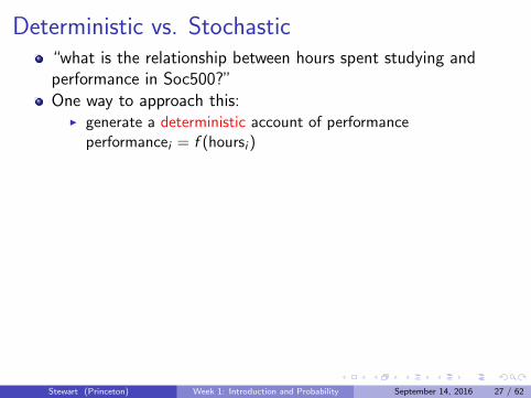
Deterministic vs. Stochastic“what is the relationship between hours spent studying andperformance in Soc500?”
One way to approach this:I generate a deterministic account of performance
performancei = f (hoursi )I but studying isn’t the only indicator of performance!I we could try to account for everything
performancei = f (hoursi ) + g(otheri ).I but that’s impossible
A better approachI Instead treat other factors as stochasticI Thus we often write it as
performancei = f (hoursi ) + εiI This allows us to have uncertainty over outcomes given our
inputs
Our way of talking about stochastic outcomes is probability.
Stewart (Princeton) Week 1: Introduction and Probability September 14, 2016 27 / 62

Deterministic vs. Stochastic“what is the relationship between hours spent studying andperformance in Soc500?”One way to approach this:
I generate a deterministic account of performanceperformancei = f (hoursi )
I but studying isn’t the only indicator of performance!I we could try to account for everything
performancei = f (hoursi ) + g(otheri ).I but that’s impossible
A better approachI Instead treat other factors as stochasticI Thus we often write it as
performancei = f (hoursi ) + εiI This allows us to have uncertainty over outcomes given our
inputs
Our way of talking about stochastic outcomes is probability.
Stewart (Princeton) Week 1: Introduction and Probability September 14, 2016 27 / 62

Deterministic vs. Stochastic“what is the relationship between hours spent studying andperformance in Soc500?”One way to approach this:
I generate a deterministic account of performanceperformancei = f (hoursi )
I but studying isn’t the only indicator of performance!
I we could try to account for everythingperformancei = f (hoursi ) + g(otheri ).
I but that’s impossible
A better approachI Instead treat other factors as stochasticI Thus we often write it as
performancei = f (hoursi ) + εiI This allows us to have uncertainty over outcomes given our
inputs
Our way of talking about stochastic outcomes is probability.
Stewart (Princeton) Week 1: Introduction and Probability September 14, 2016 27 / 62

Deterministic vs. Stochastic“what is the relationship between hours spent studying andperformance in Soc500?”One way to approach this:
I generate a deterministic account of performanceperformancei = f (hoursi )
I but studying isn’t the only indicator of performance!I we could try to account for everything
performancei = f (hoursi ) + g(otheri ).
I but that’s impossible
A better approachI Instead treat other factors as stochasticI Thus we often write it as
performancei = f (hoursi ) + εiI This allows us to have uncertainty over outcomes given our
inputs
Our way of talking about stochastic outcomes is probability.
Stewart (Princeton) Week 1: Introduction and Probability September 14, 2016 27 / 62

Deterministic vs. Stochastic“what is the relationship between hours spent studying andperformance in Soc500?”One way to approach this:
I generate a deterministic account of performanceperformancei = f (hoursi )
I but studying isn’t the only indicator of performance!I we could try to account for everything
performancei = f (hoursi ) + g(otheri ).I but that’s impossible
A better approachI Instead treat other factors as stochasticI Thus we often write it as
performancei = f (hoursi ) + εiI This allows us to have uncertainty over outcomes given our
inputs
Our way of talking about stochastic outcomes is probability.
Stewart (Princeton) Week 1: Introduction and Probability September 14, 2016 27 / 62

Deterministic vs. Stochastic“what is the relationship between hours spent studying andperformance in Soc500?”One way to approach this:
I generate a deterministic account of performanceperformancei = f (hoursi )
I but studying isn’t the only indicator of performance!I we could try to account for everything
performancei = f (hoursi ) + g(otheri ).I but that’s impossible
A better approach
I Instead treat other factors as stochasticI Thus we often write it as
performancei = f (hoursi ) + εiI This allows us to have uncertainty over outcomes given our
inputs
Our way of talking about stochastic outcomes is probability.
Stewart (Princeton) Week 1: Introduction and Probability September 14, 2016 27 / 62

Deterministic vs. Stochastic“what is the relationship between hours spent studying andperformance in Soc500?”One way to approach this:
I generate a deterministic account of performanceperformancei = f (hoursi )
I but studying isn’t the only indicator of performance!I we could try to account for everything
performancei = f (hoursi ) + g(otheri ).I but that’s impossible
A better approachI Instead treat other factors as stochastic
I Thus we often write it asperformancei = f (hoursi ) + εi
I This allows us to have uncertainty over outcomes given ourinputs
Our way of talking about stochastic outcomes is probability.
Stewart (Princeton) Week 1: Introduction and Probability September 14, 2016 27 / 62

Deterministic vs. Stochastic“what is the relationship between hours spent studying andperformance in Soc500?”One way to approach this:
I generate a deterministic account of performanceperformancei = f (hoursi )
I but studying isn’t the only indicator of performance!I we could try to account for everything
performancei = f (hoursi ) + g(otheri ).I but that’s impossible
A better approachI Instead treat other factors as stochasticI Thus we often write it as
performancei = f (hoursi ) + εi
I This allows us to have uncertainty over outcomes given ourinputs
Our way of talking about stochastic outcomes is probability.
Stewart (Princeton) Week 1: Introduction and Probability September 14, 2016 27 / 62

Deterministic vs. Stochastic“what is the relationship between hours spent studying andperformance in Soc500?”One way to approach this:
I generate a deterministic account of performanceperformancei = f (hoursi )
I but studying isn’t the only indicator of performance!I we could try to account for everything
performancei = f (hoursi ) + g(otheri ).I but that’s impossible
A better approachI Instead treat other factors as stochasticI Thus we often write it as
performancei = f (hoursi ) + εiI This allows us to have uncertainty over outcomes given our
inputs
Our way of talking about stochastic outcomes is probability.
Stewart (Princeton) Week 1: Introduction and Probability September 14, 2016 27 / 62

Deterministic vs. Stochastic“what is the relationship between hours spent studying andperformance in Soc500?”One way to approach this:
I generate a deterministic account of performanceperformancei = f (hoursi )
I but studying isn’t the only indicator of performance!I we could try to account for everything
performancei = f (hoursi ) + g(otheri ).I but that’s impossible
A better approachI Instead treat other factors as stochasticI Thus we often write it as
performancei = f (hoursi ) + εiI This allows us to have uncertainty over outcomes given our
inputs
Our way of talking about stochastic outcomes is probability.
Stewart (Princeton) Week 1: Introduction and Probability September 14, 2016 27 / 62

In Picture Form
±÷rasa
⇒
@I
€@# ••••••@a
. ÷÷.÷÷÷÷a**roao¥÷.
HE
:
•:÷ .
.÷÷÷÷¥.arrF
§egresses
Stewart (Princeton) Week 1: Introduction and Probability September 14, 2016 28 / 62

In Picture Form
±÷rasa
⇒
@I
€@# ••••••@a
. ÷÷.÷÷÷÷a**roao¥÷.
HE
:
•:÷ .
.÷÷÷÷¥.arrF
§egresses
Stewart (Princeton) Week 1: Introduction and Probability September 14, 2016 28 / 62
In Picture Form
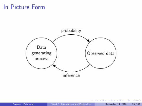
Datagenerating
processObserved data
probability
inference
Stewart (Princeton) Week 1: Introduction and Probability September 14, 2016 29 / 62

Statistical Thought Experiments
Start with probability
Allows us to contemplate world under hypothetical scenariosI hypotheticals let us ask- is the observed relationship happening
by chance or is it systematic?I it tells us what the world would look like under a certain
assumption
We will review probability today, but feel free to ask questions asneeded.
Stewart (Princeton) Week 1: Introduction and Probability September 14, 2016 30 / 62

Statistical Thought Experiments
Start with probability
Allows us to contemplate world under hypothetical scenarios
I hypotheticals let us ask- is the observed relationship happeningby chance or is it systematic?
I it tells us what the world would look like under a certainassumption
We will review probability today, but feel free to ask questions asneeded.
Stewart (Princeton) Week 1: Introduction and Probability September 14, 2016 30 / 62

Statistical Thought Experiments
Start with probability
Allows us to contemplate world under hypothetical scenariosI hypotheticals let us ask- is the observed relationship happening
by chance or is it systematic?
I it tells us what the world would look like under a certainassumption
We will review probability today, but feel free to ask questions asneeded.
Stewart (Princeton) Week 1: Introduction and Probability September 14, 2016 30 / 62

Statistical Thought Experiments
Start with probability
Allows us to contemplate world under hypothetical scenariosI hypotheticals let us ask- is the observed relationship happening
by chance or is it systematic?I it tells us what the world would look like under a certain
assumption
We will review probability today, but feel free to ask questions asneeded.
Stewart (Princeton) Week 1: Introduction and Probability September 14, 2016 30 / 62

Statistical Thought Experiments
Start with probability
Allows us to contemplate world under hypothetical scenariosI hypotheticals let us ask- is the observed relationship happening
by chance or is it systematic?I it tells us what the world would look like under a certain
assumption
We will review probability today, but feel free to ask questions asneeded.
Stewart (Princeton) Week 1: Introduction and Probability September 14, 2016 30 / 62

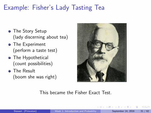
Example: Fisher’s Lady Tasting Tea
The Story Setup(lady discerning about tea)
The Experiment(perform a taste test)
The Hypothetical(count possibilities)
The Result(boom she was right)
This became the Fisher Exact Test.
Stewart (Princeton) Week 1: Introduction and Probability September 14, 2016 31 / 62

Example: Fisher’s Lady Tasting Tea
The Story Setup
(lady discerning about tea)
The Experiment(perform a taste test)
The Hypothetical(count possibilities)
The Result(boom she was right)
This became the Fisher Exact Test.
Stewart (Princeton) Week 1: Introduction and Probability September 14, 2016 31 / 62

Example: Fisher’s Lady Tasting Tea
The Story Setup(lady discerning about tea)
The Experiment(perform a taste test)
The Hypothetical(count possibilities)
The Result(boom she was right)
This became the Fisher Exact Test.
Stewart (Princeton) Week 1: Introduction and Probability September 14, 2016 31 / 62

Example: Fisher’s Lady Tasting Tea
The Story Setup(lady discerning about tea)
The Experiment
(perform a taste test)
The Hypothetical(count possibilities)
The Result(boom she was right)
This became the Fisher Exact Test.
Stewart (Princeton) Week 1: Introduction and Probability September 14, 2016 31 / 62

Example: Fisher’s Lady Tasting Tea
The Story Setup(lady discerning about tea)
The Experiment(perform a taste test)
The Hypothetical(count possibilities)
The Result(boom she was right)
This became the Fisher Exact Test.
Stewart (Princeton) Week 1: Introduction and Probability September 14, 2016 31 / 62

Example: Fisher’s Lady Tasting Tea
The Story Setup(lady discerning about tea)
The Experiment(perform a taste test)
The Hypothetical
(count possibilities)
The Result(boom she was right)
This became the Fisher Exact Test.
Stewart (Princeton) Week 1: Introduction and Probability September 14, 2016 31 / 62

Example: Fisher’s Lady Tasting Tea
The Story Setup(lady discerning about tea)
The Experiment(perform a taste test)
The Hypothetical(count possibilities)
The Result(boom she was right)
This became the Fisher Exact Test.
Stewart (Princeton) Week 1: Introduction and Probability September 14, 2016 31 / 62

Example: Fisher’s Lady Tasting Tea
The Story Setup(lady discerning about tea)
The Experiment(perform a taste test)
The Hypothetical(count possibilities)
The Result
(boom she was right)
This became the Fisher Exact Test.
Stewart (Princeton) Week 1: Introduction and Probability September 14, 2016 31 / 62

Example: Fisher’s Lady Tasting Tea
The Story Setup(lady discerning about tea)
The Experiment(perform a taste test)
The Hypothetical(count possibilities)
The Result(boom she was right)
This became the Fisher Exact Test.
Stewart (Princeton) Week 1: Introduction and Probability September 14, 2016 31 / 62

1 Welcome
2 Goals
3 Ways to Learn
4 Structure of Course
5 Introduction to ProbabilityWhat is Probability?Sample Spaces and EventsProbability FunctionsMarginal, Joint and Conditional ProbabilityBayes’ RuleIndependence
6 Fun With History
Stewart (Princeton) Week 1: Introduction and Probability September 14, 2016 32 / 62

Why Probability?
Helps us envision hypotheticals
Describes uncertainty in how the data is generated
Data Analysis: estimate probability that something will happen
Thus: we need to know how probability gives rise to data
Stewart (Princeton) Week 1: Introduction and Probability September 14, 2016 33 / 62
Intuitive Definition of Probability
While there are several interpretations of what probability is, mostmodern (post 1935 or so) researchers agree on an axiomaticdefinition of probability.
3 Axioms (Intuitive Version):
1 The probability of any particular event must be non-negative.
2 The probability of anything occurring among all possible eventsmust be 1.
3 The probability of one of many mutually exclusive eventshappening is the sum of the individual probabilities.
All the rules of probability can be derived from these axioms.
Stewart (Princeton) Week 1: Introduction and Probability September 14, 2016 34 / 62

Sample Spaces
To define probability we need to define the set of possible outcomes.
The sample space is the set of all possible outcomes, and is oftenwritten as S or Ω.
For example, if we flip a coin twice, there are four possible outcomes,
S =heads, heads, heads, tails, tails, heads, tails, tails
Thus the table in Lady Tasting Tea was defining the sample space.(Note we defined illogical guesses to be prob= 0)
Stewart (Princeton) Week 1: Introduction and Probability September 14, 2016 35 / 62

Sample Spaces
To define probability we need to define the set of possible outcomes.
The sample space is the set of all possible outcomes, and is oftenwritten as S or Ω.
For example, if we flip a coin twice, there are four possible outcomes,
S =
heads, heads, heads, tails, tails, heads, tails, tails
Thus the table in Lady Tasting Tea was defining the sample space.(Note we defined illogical guesses to be prob= 0)
Stewart (Princeton) Week 1: Introduction and Probability September 14, 2016 35 / 62

Sample Spaces
To define probability we need to define the set of possible outcomes.
The sample space is the set of all possible outcomes, and is oftenwritten as S or Ω.
For example, if we flip a coin twice, there are four possible outcomes,
S =heads, heads,
heads, tails, tails, heads, tails, tails
Thus the table in Lady Tasting Tea was defining the sample space.(Note we defined illogical guesses to be prob= 0)
Stewart (Princeton) Week 1: Introduction and Probability September 14, 2016 35 / 62

Sample Spaces
To define probability we need to define the set of possible outcomes.
The sample space is the set of all possible outcomes, and is oftenwritten as S or Ω.
For example, if we flip a coin twice, there are four possible outcomes,
S =heads, heads, heads, tails,
tails, heads, tails, tails
Thus the table in Lady Tasting Tea was defining the sample space.(Note we defined illogical guesses to be prob= 0)
Stewart (Princeton) Week 1: Introduction and Probability September 14, 2016 35 / 62

Sample Spaces
To define probability we need to define the set of possible outcomes.
The sample space is the set of all possible outcomes, and is oftenwritten as S or Ω.
For example, if we flip a coin twice, there are four possible outcomes,
S =heads, heads, heads, tails, tails, heads,
tails, tails
Thus the table in Lady Tasting Tea was defining the sample space.(Note we defined illogical guesses to be prob= 0)
Stewart (Princeton) Week 1: Introduction and Probability September 14, 2016 35 / 62

Sample Spaces
To define probability we need to define the set of possible outcomes.
The sample space is the set of all possible outcomes, and is oftenwritten as S or Ω.
For example, if we flip a coin twice, there are four possible outcomes,
S =heads, heads, heads, tails, tails, heads, tails, tails
Thus the table in Lady Tasting Tea was defining the sample space.(Note we defined illogical guesses to be prob= 0)
Stewart (Princeton) Week 1: Introduction and Probability September 14, 2016 35 / 62

Sample Spaces
To define probability we need to define the set of possible outcomes.
The sample space is the set of all possible outcomes, and is oftenwritten as S or Ω.
For example, if we flip a coin twice, there are four possible outcomes,
S =heads, heads, heads, tails, tails, heads, tails, tails
Thus the table in Lady Tasting Tea was defining the sample space.
(Note we defined illogical guesses to be prob= 0)
Stewart (Princeton) Week 1: Introduction and Probability September 14, 2016 35 / 62

Sample Spaces
To define probability we need to define the set of possible outcomes.
The sample space is the set of all possible outcomes, and is oftenwritten as S or Ω.
For example, if we flip a coin twice, there are four possible outcomes,
S =heads, heads, heads, tails, tails, heads, tails, tails
Thus the table in Lady Tasting Tea was defining the sample space.(Note we defined illogical guesses to be prob= 0)
Stewart (Princeton) Week 1: Introduction and Probability September 14, 2016 35 / 62

A Running Visual Metaphor
Imagine that we sample an apple from a bag.Looking in the bag we see:
The sample space is:
Stewart (Princeton) Week 1: Introduction and Probability September 14, 2016 36 / 62

A Running Visual Metaphor
Imagine that we sample an apple from a bag.
Looking in the bag we see:
The sample space is:
Stewart (Princeton) Week 1: Introduction and Probability September 14, 2016 36 / 62

A Running Visual Metaphor
Imagine that we sample an apple from a bag.Looking in the bag we see:
The sample space is:
Stewart (Princeton) Week 1: Introduction and Probability September 14, 2016 36 / 62

A Running Visual Metaphor
Imagine that we sample an apple from a bag.Looking in the bag we see:
The sample space is:
Stewart (Princeton) Week 1: Introduction and Probability September 14, 2016 36 / 62

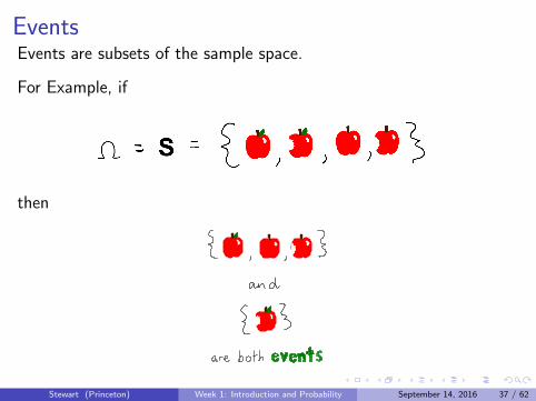
EventsEvents are subsets of the sample space.
For Example, if
then
←a given
, )
and
rain are both . T.B.DMBB.GG.
.
Stewart (Princeton) Week 1: Introduction and Probability September 14, 2016 37 / 62

EventsEvents are subsets of the sample space.
For Example, if
then
←a given
, )
and
rain are both . T.B.DMBB.GG.
.
Stewart (Princeton) Week 1: Introduction and Probability September 14, 2016 37 / 62
EventsEvents are subsets of the sample space.
For Example, if
then
←a given
, )
and
rain are both . T.B.DMBB.GG.
.
Stewart (Princeton) Week 1: Introduction and Probability September 14, 2016 37 / 62

Events Are a Kind of Set
Sets are collections of things, in this case collections of outcomes
One way to define an event is to describe the common property thatall of the outcomes share. We write this as
ω|ω satisfies P,
where P is the property that they all share.
Stewart (Princeton) Week 1: Introduction and Probability September 14, 2016 38 / 62

Events Are a Kind of SetSets are collections of things, in this case collections of outcomes
One way to define an event is to describe the common property thatall of the outcomes share. We write this as
ω|ω satisfies P,
where P is the property that they all share.
Stewart (Princeton) Week 1: Introduction and Probability September 14, 2016 38 / 62
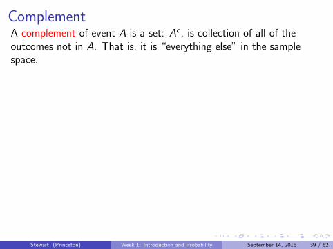
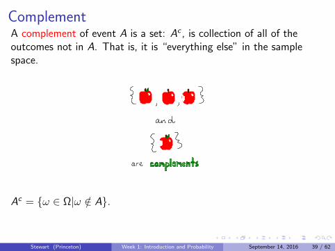
ComplementA complement of event A is a set: Ac , is collection of all of theoutcomes not in A. That is, it is “everything else” in the samplespace.
←a given
, )
and
againare
.
Ac = ω ∈ Ω|ω /∈ A.Important complement: Ωc = ∅, where ∅ is the empty set—it’s justthe event that nothing happens.
Stewart (Princeton) Week 1: Introduction and Probability September 14, 2016 39 / 62
ComplementA complement of event A is a set: Ac , is collection of all of theoutcomes not in A. That is, it is “everything else” in the samplespace.
←a given
, )
and
againare
.
Ac = ω ∈ Ω|ω /∈ A.
Important complement: Ωc = ∅, where ∅ is the empty set—it’s justthe event that nothing happens.
Stewart (Princeton) Week 1: Introduction and Probability September 14, 2016 39 / 62

ComplementA complement of event A is a set: Ac , is collection of all of theoutcomes not in A. That is, it is “everything else” in the samplespace.
←a given
, )
and
againare
.
Ac = ω ∈ Ω|ω /∈ A.Important complement: Ωc = ∅, where ∅ is the empty set—it’s justthe event that nothing happens.
Stewart (Princeton) Week 1: Introduction and Probability September 14, 2016 39 / 62

Operations on Events
The union of two events, A and B is the event that A or B occurs:
• . u *on =
air,
#Mina,air
A ∪ B = ω|ω ∈ A or ω ∈ B.
The intersection of two events, A and B is the event that both A andB occur:
• s.no#go=
ease A ∩ B = ω|ω ∈ A and ω ∈ B.
Stewart (Princeton) Week 1: Introduction and Probability September 14, 2016 40 / 62

Operations on Events
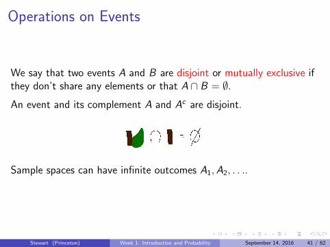
We say that two events A and B are disjoint or mutually exclusive ifthey don’t share any elements or that A ∩ B = ∅.
An event and its complement A and Ac are disjoint.
Sample spaces can have infinite outcomes A1,A2, . . ..
Stewart (Princeton) Week 1: Introduction and Probability September 14, 2016 41 / 62

Operations on Events
We say that two events A and B are disjoint or mutually exclusive ifthey don’t share any elements or that A ∩ B = ∅.
An event and its complement A and Ac are disjoint.
Sample spaces can have infinite outcomes A1,A2, . . ..
Stewart (Princeton) Week 1: Introduction and Probability September 14, 2016 41 / 62

Probability FunctionA probability function P(·) is a function defined over all subsets of asample space S that satisfies the following three axioms:
1 P(A) ≥ 0 for all A in the setof all events.
nonnegativity
2 P(S) = 1
normalization
3 if events A1,A2, . . . aremutually exclusive thenP(⋃∞
i=1 Ai) =∑∞
i=1 P(Ai).
additivity
All the rules of probability can be derived from these axioms.
Intuition: probability as allocating chunks of a unit-long stick.
Stewart (Princeton) Week 1: Introduction and Probability September 14, 2016 42 / 62

Probability FunctionA probability function P(·) is a function defined over all subsets of asample space S that satisfies the following three axioms:
1 P(A) ≥ 0 for all A in the setof all events.
nonnegativity
2 P(S) = 1
normalization
3 if events A1,A2, . . . aremutually exclusive thenP(⋃∞
i=1 Ai) =∑∞
i=1 P(Ai).
additivity
B. P(89 ) =
-
.
5
All the rules of probability can be derived from these axioms.
Intuition: probability as allocating chunks of a unit-long stick.
Stewart (Princeton) Week 1: Introduction and Probability September 14, 2016 42 / 62

Probability FunctionA probability function P(·) is a function defined over all subsets of asample space S that satisfies the following three axioms:
1 P(A) ≥ 0 for all A in the setof all events. nonnegativity
2 P(S) = 1
normalization
3 if events A1,A2, . . . aremutually exclusive thenP(⋃∞
i=1 Ai) =∑∞
i=1 P(Ai).
additivity
B.P (89 ) =
-
.
5
399k.
P ( air,
raise,
@,Bin ) = 1
All the rules of probability can be derived from these axioms.
Intuition: probability as allocating chunks of a unit-long stick.
Stewart (Princeton) Week 1: Introduction and Probability September 14, 2016 42 / 62

Probability FunctionA probability function P(·) is a function defined over all subsets of asample space S that satisfies the following three axioms:
1 P(A) ≥ 0 for all A in the setof all events. nonnegativity
2 P(S) = 1 normalization
3 if events A1,A2, . . . aremutually exclusive thenP(⋃∞
i=1 Ai) =∑∞
i=1 P(Ai).
additivity
B.P (89 ) =
-
.
5
399k.
P ( give.ba,
@an) = 1
B..
P (given
) = P ( Aip ) +
Praa)
nqwhen a and he# are
mutually exclusive.
All the rules of probability can be derived from these axioms.
Intuition: probability as allocating chunks of a unit-long stick.
Stewart (Princeton) Week 1: Introduction and Probability September 14, 2016 42 / 62

Probability FunctionA probability function P(·) is a function defined over all subsets of asample space S that satisfies the following three axioms:
1 P(A) ≥ 0 for all A in the setof all events. nonnegativity
2 P(S) = 1 normalization
3 if events A1,A2, . . . aremutually exclusive thenP(⋃∞
i=1 Ai) =∑∞
i=1 P(Ai).additivity
B.P (89 ) =
-
.
5
399k.
P ( give.ba,
@an) = 1
B..
P (given
) = P ( Aip ) +
Praa)
nqwhen a and he# are
mutually exclusive.
All the rules of probability can be derived from these axioms.
Intuition: probability as allocating chunks of a unit-long stick.
Stewart (Princeton) Week 1: Introduction and Probability September 14, 2016 42 / 62

A Brief Word on Interpretation
Massive debate on interpretation:
Subjective InterpretationI Example: The probability of drawing 5 red cards out of 10
drawn from a deck of cards is whatever you want it to be. But...I If you don’t follow the axioms, a bookie can beat youI There is a correct way to update your beliefs with data.
Frequency InterpretationI Probability of is the relative frequency with which an event
would occur if the process were repeated a large number oftimes under similar conditions.
I Example: The probability of drawing 5 red cards out of 10drawn from a deck of cards is the frequency with which thisevent occurs in repeated samples of 10 cards.
Stewart (Princeton) Week 1: Introduction and Probability September 14, 2016 43 / 62

A Brief Word on Interpretation
Massive debate on interpretation:
Subjective Interpretation
I Example: The probability of drawing 5 red cards out of 10drawn from a deck of cards is whatever you want it to be. But...
I If you don’t follow the axioms, a bookie can beat youI There is a correct way to update your beliefs with data.
Frequency InterpretationI Probability of is the relative frequency with which an event
would occur if the process were repeated a large number oftimes under similar conditions.
I Example: The probability of drawing 5 red cards out of 10drawn from a deck of cards is the frequency with which thisevent occurs in repeated samples of 10 cards.
Stewart (Princeton) Week 1: Introduction and Probability September 14, 2016 43 / 62

A Brief Word on Interpretation
Massive debate on interpretation:
Subjective InterpretationI Example: The probability of drawing 5 red cards out of 10
drawn from a deck of cards is whatever you want it to be.
But...I If you don’t follow the axioms, a bookie can beat youI There is a correct way to update your beliefs with data.
Frequency InterpretationI Probability of is the relative frequency with which an event
would occur if the process were repeated a large number oftimes under similar conditions.
I Example: The probability of drawing 5 red cards out of 10drawn from a deck of cards is the frequency with which thisevent occurs in repeated samples of 10 cards.
Stewart (Princeton) Week 1: Introduction and Probability September 14, 2016 43 / 62

A Brief Word on Interpretation
Massive debate on interpretation:
Subjective InterpretationI Example: The probability of drawing 5 red cards out of 10
drawn from a deck of cards is whatever you want it to be. But...
I If you don’t follow the axioms, a bookie can beat youI There is a correct way to update your beliefs with data.
Frequency InterpretationI Probability of is the relative frequency with which an event
would occur if the process were repeated a large number oftimes under similar conditions.
I Example: The probability of drawing 5 red cards out of 10drawn from a deck of cards is the frequency with which thisevent occurs in repeated samples of 10 cards.
Stewart (Princeton) Week 1: Introduction and Probability September 14, 2016 43 / 62

A Brief Word on Interpretation
Massive debate on interpretation:
Subjective InterpretationI Example: The probability of drawing 5 red cards out of 10
drawn from a deck of cards is whatever you want it to be. But...I If you don’t follow the axioms, a bookie can beat you
I There is a correct way to update your beliefs with data.
Frequency InterpretationI Probability of is the relative frequency with which an event
would occur if the process were repeated a large number oftimes under similar conditions.
I Example: The probability of drawing 5 red cards out of 10drawn from a deck of cards is the frequency with which thisevent occurs in repeated samples of 10 cards.
Stewart (Princeton) Week 1: Introduction and Probability September 14, 2016 43 / 62

A Brief Word on Interpretation
Massive debate on interpretation:
Subjective InterpretationI Example: The probability of drawing 5 red cards out of 10
drawn from a deck of cards is whatever you want it to be. But...I If you don’t follow the axioms, a bookie can beat youI There is a correct way to update your beliefs with data.
Frequency InterpretationI Probability of is the relative frequency with which an event
would occur if the process were repeated a large number oftimes under similar conditions.
I Example: The probability of drawing 5 red cards out of 10drawn from a deck of cards is the frequency with which thisevent occurs in repeated samples of 10 cards.
Stewart (Princeton) Week 1: Introduction and Probability September 14, 2016 43 / 62

A Brief Word on Interpretation
Massive debate on interpretation:
Subjective InterpretationI Example: The probability of drawing 5 red cards out of 10
drawn from a deck of cards is whatever you want it to be. But...I If you don’t follow the axioms, a bookie can beat youI There is a correct way to update your beliefs with data.
Frequency Interpretation
I Probability of is the relative frequency with which an eventwould occur if the process were repeated a large number oftimes under similar conditions.
I Example: The probability of drawing 5 red cards out of 10drawn from a deck of cards is the frequency with which thisevent occurs in repeated samples of 10 cards.
Stewart (Princeton) Week 1: Introduction and Probability September 14, 2016 43 / 62

A Brief Word on Interpretation
Massive debate on interpretation:
Subjective InterpretationI Example: The probability of drawing 5 red cards out of 10
drawn from a deck of cards is whatever you want it to be. But...I If you don’t follow the axioms, a bookie can beat youI There is a correct way to update your beliefs with data.
Frequency InterpretationI Probability of is the relative frequency with which an event
would occur if the process were repeated a large number oftimes under similar conditions.
I Example: The probability of drawing 5 red cards out of 10drawn from a deck of cards is the frequency with which thisevent occurs in repeated samples of 10 cards.
Stewart (Princeton) Week 1: Introduction and Probability September 14, 2016 43 / 62

A Brief Word on Interpretation
Massive debate on interpretation:
Subjective InterpretationI Example: The probability of drawing 5 red cards out of 10
drawn from a deck of cards is whatever you want it to be. But...I If you don’t follow the axioms, a bookie can beat youI There is a correct way to update your beliefs with data.
Frequency InterpretationI Probability of is the relative frequency with which an event
would occur if the process were repeated a large number oftimes under similar conditions.
I Example: The probability of drawing 5 red cards out of 10drawn from a deck of cards is the frequency with which thisevent occurs in repeated samples of 10 cards.
Stewart (Princeton) Week 1: Introduction and Probability September 14, 2016 43 / 62

Marginal and Joint Probability
So far we have only considered situations where we are interested inthe probability of a single event A occurring. We’ve denoted thisP(A). P(A) is sometimes called a marginal probability.
Suppose we are now in a situation where we would like to express theprobability that an event A and an event B occur. This quantity iswritten as P(A ∩ B), P(B ∩ A), P(A,B), or P(B ,A) and is the jointprobability of A and B .
Stewart (Princeton) Week 1: Introduction and Probability September 14, 2016 44 / 62

ap(
a.)= ?
.ringing.*air
.rain. #*@a
. ¥589
←. • . µp(
qq.pe#)=? a a
Stewart (Princeton) Week 1: Introduction and Probability September 14, 2016 45 / 62

Conditional Probability
The “soul of statistics”If P(A) > 0 then the probability of B conditional on A can be writtenas
P(B |A) =P(A,B)
P(A)
This implies that
P(A,B) = P(A)× P(B |A)
Stewart (Princeton) Week 1: Introduction and Probability September 14, 2016 46 / 62

Conditional Probability
The “soul of statistics”
If P(A) > 0 then the probability of B conditional on A can be writtenas
P(B |A) =P(A,B)
P(A)
This implies that
P(A,B) = P(A)× P(B |A)
Stewart (Princeton) Week 1: Introduction and Probability September 14, 2016 46 / 62

Conditional Probability
The “soul of statistics”If P(A) > 0 then the probability of B conditional on A can be writtenas
P(B |A) =P(A,B)
P(A)
This implies that
P(A,B) = P(A)× P(B |A)
Stewart (Princeton) Week 1: Introduction and Probability September 14, 2016 46 / 62

Conditional Probability
The “soul of statistics”If P(A) > 0 then the probability of B conditional on A can be writtenas
P(B |A) =P(A,B)
P(A)
This implies that
P(A,B) = P(A)× P(B |A)
Stewart (Princeton) Week 1: Introduction and Probability September 14, 2016 46 / 62

Conditional Probability
The “soul of statistics”If P(A) > 0 then the probability of B conditional on A can be writtenas
P(B |A) =P(A,B)
P(A)
This implies that
P(A,B) = P(A)× P(B |A)
Stewart (Princeton) Week 1: Introduction and Probability September 14, 2016 46 / 62

Conditional Probability
The “soul of statistics”If P(A) > 0 then the probability of B conditional on A can be writtenas
P(B |A) =P(A,B)
P(A)
This implies that
P(A,B) = P(A)× P(B |A)
Stewart (Princeton) Week 1: Introduction and Probability September 14, 2016 46 / 62

Conditional Probability: A Visual Example
Parsa.
t.io) =
PC.ae#dpl*abidsgrain
.
• agear• •a *oroaivoiv
Stewart (Princeton) Week 1: Introduction and Probability September 14, 2016 47 / 62

Conditional Probability: A Visual Example
Parsa.
t.io) =
PC.ae#dpl*abidsgrain
.
• agear• •a *oroaivoiv
Stewart (Princeton) Week 1: Introduction and Probability September 14, 2016 47 / 62

Conditional Probability: A Visual Example
Parsa.
t.io) =
PC.ae#dpl*abidsgrain
.
• agear• •a *oroaivoiv
Stewart (Princeton) Week 1: Introduction and Probability September 14, 2016 47 / 62

A Card Player’s Example
If we randomly draw two cards from a standard 52 card deck anddefine the eventsA = King on Draw 1 and B = King on Draw 2, then
P(A) = 4/52
P(B |A) = 3/51
P(A,B) = P(A)× P(B |A) = 4/52× 3/51 ≈ .0045
Stewart (Princeton) Week 1: Introduction and Probability September 14, 2016 48 / 62

A Card Player’s Example
If we randomly draw two cards from a standard 52 card deck anddefine the eventsA = King on Draw 1 and B = King on Draw 2, then
P(A) =
4/52
P(B |A) = 3/51
P(A,B) = P(A)× P(B |A) = 4/52× 3/51 ≈ .0045
Stewart (Princeton) Week 1: Introduction and Probability September 14, 2016 48 / 62

A Card Player’s Example
If we randomly draw two cards from a standard 52 card deck anddefine the eventsA = King on Draw 1 and B = King on Draw 2, then
P(A) = 4/52
P(B |A) = 3/51
P(A,B) = P(A)× P(B |A) = 4/52× 3/51 ≈ .0045
Stewart (Princeton) Week 1: Introduction and Probability September 14, 2016 48 / 62

A Card Player’s Example
If we randomly draw two cards from a standard 52 card deck anddefine the eventsA = King on Draw 1 and B = King on Draw 2, then
P(A) = 4/52
P(B |A) =
3/51
P(A,B) = P(A)× P(B |A) = 4/52× 3/51 ≈ .0045
Stewart (Princeton) Week 1: Introduction and Probability September 14, 2016 48 / 62

A Card Player’s Example
If we randomly draw two cards from a standard 52 card deck anddefine the eventsA = King on Draw 1 and B = King on Draw 2, then
P(A) = 4/52
P(B |A) = 3/51
P(A,B) = P(A)× P(B |A) = 4/52× 3/51 ≈ .0045
Stewart (Princeton) Week 1: Introduction and Probability September 14, 2016 48 / 62
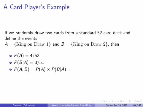
A Card Player’s Example
If we randomly draw two cards from a standard 52 card deck anddefine the eventsA = King on Draw 1 and B = King on Draw 2, then
P(A) = 4/52
P(B |A) = 3/51
P(A,B) = P(A)× P(B |A) =
4/52× 3/51 ≈ .0045
Stewart (Princeton) Week 1: Introduction and Probability September 14, 2016 48 / 62

A Card Player’s Example
If we randomly draw two cards from a standard 52 card deck anddefine the eventsA = King on Draw 1 and B = King on Draw 2, then
P(A) = 4/52
P(B |A) = 3/51
P(A,B) = P(A)× P(B |A) = 4/52× 3/51 ≈ .0045
Stewart (Princeton) Week 1: Introduction and Probability September 14, 2016 48 / 62

Law of Total Probability (LTP)
With 2 Events:
P(B) = P(B ,A) + P(B ,Ac)
= P(B |A)× P(A) + P(B |Ac)× P(Ac)
Stewart (Princeton) Week 1: Introduction and Probability September 14, 2016 49 / 62

Recall, if we randomly draw two cards from a standard 52 card deckand define the events A = King on Draw 1 andB = King on Draw 2, then
P(A) = 4/52
P(B |A) = 3/51
P(A,B) = P(A)× P(B |A) = 4/52× 3/51
Question: P(B) =?
Stewart (Princeton) Week 1: Introduction and Probability September 14, 2016 50 / 62

Confirming Intuition with the LTP
P(B) = P(B ,A) + P(B ,Ac)
= P(B |A)× P(A) + P(B |Ac)× P(Ac)
P(B) = 3/51× 1/13 + 4/51× 12/13
=3 + 48
51× 13=
1
13=
4
52
Stewart (Princeton) Week 1: Introduction and Probability September 14, 2016 51 / 62

Confirming Intuition with the LTP
P(B) = P(B ,A) + P(B ,Ac)
= P(B |A)× P(A) + P(B |Ac)× P(Ac)
P(B) = 3/51× 1/13 + 4/51× 12/13
=3 + 48
51× 13=
1
13=
4
52
Stewart (Princeton) Week 1: Introduction and Probability September 14, 2016 51 / 62

Confirming Intuition with the LTP
P(B) = P(B ,A) + P(B ,Ac)
= P(B |A)× P(A) + P(B |Ac)× P(Ac)
P(B) = 3/51× 1/13 + 4/51× 12/13
=3 + 48
51× 13=
1
13=
4
52
Stewart (Princeton) Week 1: Introduction and Probability September 14, 2016 51 / 62

Example: Voter MobilizationSuppose that we have put together a voter mobilization campaignand we want to know what the probability of voting is after thecampaign: Pr[vote].
We know the following:
Pr(vote|mobilized) = 0.75
Pr(vote|not mobilized) = 0.15
Pr(mobilized) = 0.6 and so Pr( not mobilized) = 0.4
Note that mobilization partitions the data. Everyone is eithermobilized or not. Thus, we can apply the LTP:
Pr(vote) = Pr(vote|mobilized) Pr(mobilized)+
Pr(vote|not mobilized) Pr(not mobilized)
=0.75× 0.6 + 0.15× 0.4
=.51
Stewart (Princeton) Week 1: Introduction and Probability September 14, 2016 52 / 62

Example: Voter MobilizationSuppose that we have put together a voter mobilization campaignand we want to know what the probability of voting is after thecampaign: Pr[vote]. We know the following:
Pr(vote|mobilized) = 0.75
Pr(vote|not mobilized) = 0.15
Pr(mobilized) = 0.6 and so Pr( not mobilized) = 0.4
Note that mobilization partitions the data. Everyone is eithermobilized or not.
Thus, we can apply the LTP:
Pr(vote) = Pr(vote|mobilized) Pr(mobilized)+
Pr(vote|not mobilized) Pr(not mobilized)
=0.75× 0.6 + 0.15× 0.4
=.51
Stewart (Princeton) Week 1: Introduction and Probability September 14, 2016 52 / 62

Example: Voter MobilizationSuppose that we have put together a voter mobilization campaignand we want to know what the probability of voting is after thecampaign: Pr[vote]. We know the following:
Pr(vote|mobilized) = 0.75
Pr(vote|not mobilized) = 0.15
Pr(mobilized) = 0.6 and so Pr( not mobilized) = 0.4
Note that mobilization partitions the data. Everyone is eithermobilized or not. Thus, we can apply the LTP:
Pr(vote) = Pr(vote|mobilized) Pr(mobilized)+
Pr(vote|not mobilized) Pr(not mobilized)
=0.75× 0.6 + 0.15× 0.4
=.51
Stewart (Princeton) Week 1: Introduction and Probability September 14, 2016 52 / 62

Example: Voter MobilizationSuppose that we have put together a voter mobilization campaignand we want to know what the probability of voting is after thecampaign: Pr[vote]. We know the following:
Pr(vote|mobilized) = 0.75
Pr(vote|not mobilized) = 0.15
Pr(mobilized) = 0.6 and so Pr( not mobilized) = 0.4
Note that mobilization partitions the data. Everyone is eithermobilized or not. Thus, we can apply the LTP:
Pr(vote) = Pr(vote|mobilized) Pr(mobilized)+
Pr(vote|not mobilized) Pr(not mobilized)
=0.75× 0.6 + 0.15× 0.4
=.51
Stewart (Princeton) Week 1: Introduction and Probability September 14, 2016 52 / 62
Bayes’ Rule
Often we have information about Pr(B |A), but require Pr(A|B)instead.
When this happens, always think: Bayes’ rule
Bayes’ rule: if Pr(B) > 0, then:
Pr(A|B) =Pr(B |A) Pr(A)
Pr(B)
Proof: combine the multiplication rulePr(B |A) Pr(A) = P(A ∩ B), and the definition of conditionalprobability
Stewart (Princeton) Week 1: Introduction and Probability September 14, 2016 53 / 62

Bayes’ Rule Mechanics
... .:@ =P.cat#a..)p.h..)
Pl I )posedbirdsgo.nu
.
• •aired• •areas
aimedStewart (Princeton) Week 1: Introduction and Probability September 14, 2016 54 / 62

Bayes’ Rule Mechanics
... .:@ =P.cat#a..)p.h..)
Pl I )posedbirdsgo.nu
.
• •aired• •areas
aimedStewart (Princeton) Week 1: Introduction and Probability September 14, 2016 54 / 62
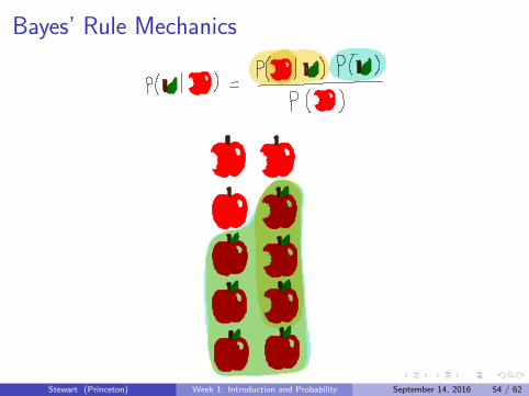
Bayes’ Rule Mechanics
... .:@ =P.cat#a..)p.h..)
Pl I )posedbirdsgo.nu
.
• •aired• •areas
aimedStewart (Princeton) Week 1: Introduction and Probability September 14, 2016 54 / 62

Bayes’ Rule Mechanics
... .:@ =P.cat#a..)p.h..)
Pl I )posedbirdsgo.nu
.
• •aired• •areas
aimedStewart (Princeton) Week 1: Introduction and Probability September 14, 2016 54 / 62

Bayes’ Rule Example
b. . .Baird .•am•••r•g
.B. . . p.
• 76.5% of female
)-| billionaires inherited their
fortunes, compared to
24.5% of male billionaires
Women Men . So is p( woman ) inherited billions )
greater than Plmanlinherited billions ) ?
Stewart (Princeton) Week 1: Introduction and Probability September 14, 2016 55 / 62

Bayes’ Rule Example
% of female
)-| billionaires inherited their
fortunes, compared to
24.5% of male billionaires
Women Men . So is P( woman ) inherited billions ),
greater than Plmanlinherited billions ).
P( WII )=P(I1W)P(w)P(I )÷ei÷ml÷÷tet
=• |
* Data source : Billionaires characteristics database
Stewart (Princeton) Week 1: Introduction and Probability September 14, 2016 55 / 62

Example: Race and Names
Enos (2015): how do we identify a person’s race from theirname?
First, note that the Census collects information on thedistribution of names by race.
For example, Washington is the most common last name amongAfrican-Americans in America:
I Pr(AfAm) = 0.132I Pr(not AfAm) = 1− Pr(AfAm) = .868I Pr(Washington|AfAm) = 0.00378I Pr(Washington|not AfAm) = 0.000061
We can now use Bayes’ Rule
Pr(AfAm|Wash) =Pr(Wash|AfAm) Pr(AfAm)
Pr(Wash)
Stewart (Princeton) Week 1: Introduction and Probability September 14, 2016 56 / 62

Example: Race and Names
Enos (2015): how do we identify a person’s race from theirname?
First, note that the Census collects information on thedistribution of names by race.
For example, Washington is the most common last name amongAfrican-Americans in America:
I Pr(AfAm) = 0.132
I Pr(not AfAm) = 1− Pr(AfAm) = .868I Pr(Washington|AfAm) = 0.00378I Pr(Washington|not AfAm) = 0.000061
We can now use Bayes’ Rule
Pr(AfAm|Wash) =Pr(Wash|AfAm) Pr(AfAm)
Pr(Wash)
Stewart (Princeton) Week 1: Introduction and Probability September 14, 2016 56 / 62

Example: Race and Names
Enos (2015): how do we identify a person’s race from theirname?
First, note that the Census collects information on thedistribution of names by race.
For example, Washington is the most common last name amongAfrican-Americans in America:
I Pr(AfAm) = 0.132I Pr(not AfAm) = 1− Pr(AfAm) = .868
I Pr(Washington|AfAm) = 0.00378I Pr(Washington|not AfAm) = 0.000061
We can now use Bayes’ Rule
Pr(AfAm|Wash) =Pr(Wash|AfAm) Pr(AfAm)
Pr(Wash)
Stewart (Princeton) Week 1: Introduction and Probability September 14, 2016 56 / 62

Example: Race and Names
Enos (2015): how do we identify a person’s race from theirname?
First, note that the Census collects information on thedistribution of names by race.
For example, Washington is the most common last name amongAfrican-Americans in America:
I Pr(AfAm) = 0.132I Pr(not AfAm) = 1− Pr(AfAm) = .868I Pr(Washington|AfAm) = 0.00378
I Pr(Washington|not AfAm) = 0.000061
We can now use Bayes’ Rule
Pr(AfAm|Wash) =Pr(Wash|AfAm) Pr(AfAm)
Pr(Wash)
Stewart (Princeton) Week 1: Introduction and Probability September 14, 2016 56 / 62

Example: Race and Names
Enos (2015): how do we identify a person’s race from theirname?
First, note that the Census collects information on thedistribution of names by race.
For example, Washington is the most common last name amongAfrican-Americans in America:
I Pr(AfAm) = 0.132I Pr(not AfAm) = 1− Pr(AfAm) = .868I Pr(Washington|AfAm) = 0.00378I Pr(Washington|not AfAm) = 0.000061
We can now use Bayes’ Rule
Pr(AfAm|Wash) =Pr(Wash|AfAm) Pr(AfAm)
Pr(Wash)
Stewart (Princeton) Week 1: Introduction and Probability September 14, 2016 56 / 62

Example: Race and Names
Enos (2015): how do we identify a person’s race from theirname?
First, note that the Census collects information on thedistribution of names by race.
For example, Washington is the most common last name amongAfrican-Americans in America:
I Pr(AfAm) = 0.132I Pr(not AfAm) = 1− Pr(AfAm) = .868I Pr(Washington|AfAm) = 0.00378I Pr(Washington|not AfAm) = 0.000061
We can now use Bayes’ Rule
Pr(AfAm|Wash) =Pr(Wash|AfAm) Pr(AfAm)
Pr(Wash)
Stewart (Princeton) Week 1: Introduction and Probability September 14, 2016 56 / 62

Example: Race and Names
Note we don’t have the probability of the name Washington.
Remember that we can calculate it from the LTP since the setsAfrican-American and not African-American partition the samplespace:
Pr(Wash|AfAm) Pr(AfAm)
Pr(Wash)=
Pr(Wash|AfAm) Pr(AfAm)
Pr(Wash|AfAm) Pr(AfAm) + Pr(Wash|not AfAm) Pr(not AfAm)
=0.132× 0.00378
0.132× 0.00378 + .868× 0.000061
≈ 0.9
Stewart (Princeton) Week 1: Introduction and Probability September 14, 2016 57 / 62

Independence
Intuitive DefinitionEvents A and B are independent if knowing whether A occurredprovides no information about whether B occurred.
Formal Definition
P(A,B) = P(A)P(B) =⇒ A⊥⊥B
With all the usual > 0 restrictions, this implies
P(A|B) = P(A)
P(B |A) = P(B)
Independence is a massively important concept in statistics.
Stewart (Princeton) Week 1: Introduction and Probability September 14, 2016 58 / 62

Independence
Intuitive Definition
Events A and B are independent if knowing whether A occurredprovides no information about whether B occurred.
Formal Definition
P(A,B) = P(A)P(B) =⇒ A⊥⊥B
With all the usual > 0 restrictions, this implies
P(A|B) = P(A)
P(B |A) = P(B)
Independence is a massively important concept in statistics.
Stewart (Princeton) Week 1: Introduction and Probability September 14, 2016 58 / 62

Independence
Intuitive DefinitionEvents A and B are independent if knowing whether A occurredprovides no information about whether B occurred.
Formal Definition
P(A,B) = P(A)P(B) =⇒ A⊥⊥B
With all the usual > 0 restrictions, this implies
P(A|B) = P(A)
P(B |A) = P(B)
Independence is a massively important concept in statistics.
Stewart (Princeton) Week 1: Introduction and Probability September 14, 2016 58 / 62

Independence
Intuitive DefinitionEvents A and B are independent if knowing whether A occurredprovides no information about whether B occurred.
Formal Definition
P(A,B) = P(A)P(B) =⇒ A⊥⊥B
With all the usual > 0 restrictions, this implies
P(A|B) = P(A)
P(B |A) = P(B)
Independence is a massively important concept in statistics.
Stewart (Princeton) Week 1: Introduction and Probability September 14, 2016 58 / 62
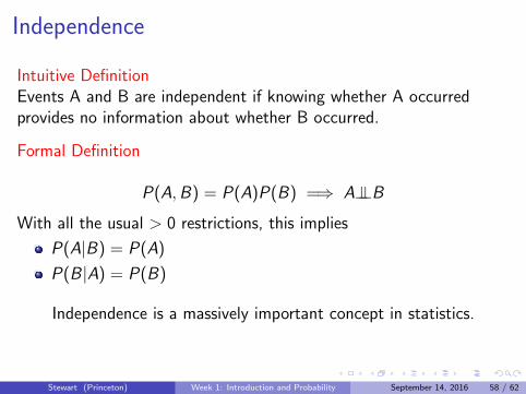
Independence
Intuitive DefinitionEvents A and B are independent if knowing whether A occurredprovides no information about whether B occurred.
Formal Definition
P(A,B) = P(A)P(B) =⇒ A⊥⊥B
With all the usual > 0 restrictions, this implies
P(A|B) = P(A)
P(B |A) = P(B)
Independence is a massively important concept in statistics.
Stewart (Princeton) Week 1: Introduction and Probability September 14, 2016 58 / 62

Next Week
Random Variables
ReadingI Aronow and Miller (1.1) on Random EventsI Aronow and Miller (1.2-2.3) on Probability Theory,
Summarizing DistributionsI Optional: Blitzstein and Hwang Chapters 1-1.3 (probability),
2-2.5 (conditional probability), 3-3.2 (random variables), 4-4.2(expectation), 4.4-4.6 (indicator rv, LOTUS, variance), 7.0-7.3(joint distributions)
I Optional: Imai Chapter 6 (probability)
A word from your preceptors
Stewart (Princeton) Week 1: Introduction and Probability September 14, 2016 59 / 62

Next Week
Random Variables
Reading
I Aronow and Miller (1.1) on Random EventsI Aronow and Miller (1.2-2.3) on Probability Theory,
Summarizing DistributionsI Optional: Blitzstein and Hwang Chapters 1-1.3 (probability),
2-2.5 (conditional probability), 3-3.2 (random variables), 4-4.2(expectation), 4.4-4.6 (indicator rv, LOTUS, variance), 7.0-7.3(joint distributions)
I Optional: Imai Chapter 6 (probability)
A word from your preceptors
Stewart (Princeton) Week 1: Introduction and Probability September 14, 2016 59 / 62

Next Week
Random Variables
ReadingI Aronow and Miller (1.1) on Random EventsI Aronow and Miller (1.2-2.3) on Probability Theory,
Summarizing DistributionsI Optional: Blitzstein and Hwang Chapters 1-1.3 (probability),
2-2.5 (conditional probability), 3-3.2 (random variables), 4-4.2(expectation), 4.4-4.6 (indicator rv, LOTUS, variance), 7.0-7.3(joint distributions)
I Optional: Imai Chapter 6 (probability)
A word from your preceptors
Stewart (Princeton) Week 1: Introduction and Probability September 14, 2016 59 / 62

Next Week
Random Variables
ReadingI Aronow and Miller (1.1) on Random EventsI Aronow and Miller (1.2-2.3) on Probability Theory,
Summarizing DistributionsI Optional: Blitzstein and Hwang Chapters 1-1.3 (probability),
2-2.5 (conditional probability), 3-3.2 (random variables), 4-4.2(expectation), 4.4-4.6 (indicator rv, LOTUS, variance), 7.0-7.3(joint distributions)
I Optional: Imai Chapter 6 (probability)
A word from your preceptors
Stewart (Princeton) Week 1: Introduction and Probability September 14, 2016 59 / 62

Fun With
Stewart (Princeton) Week 1: Introduction and Probability September 14, 2016 60 / 62
Fun with
History
Stewart (Princeton) Week 1: Introduction and Probability September 14, 2016 61 / 62

Fun with History
Stewart (Princeton) Week 1: Introduction and Probability September 14, 2016 61 / 62

Fun with History
Legendre
Stewart (Princeton) Week 1: Introduction and Probability September 14, 2016 61 / 62

Fun with History
Gauss
Stewart (Princeton) Week 1: Introduction and Probability September 14, 2016 61 / 62

Fun with History
Quetelet
Stewart (Princeton) Week 1: Introduction and Probability September 14, 2016 61 / 62

Fun with History
Galton
Stewart (Princeton) Week 1: Introduction and Probability September 14, 2016 61 / 62

References
Enos, Ryan D. ”What the demolition of public housing teachesus about the impact of racial threat on political behavior.”American Journal of Political Science (2015).
J. Andrew Harris “Whats in a Name? A Method for ExtractingInformation about Ethnicity from Names” Political Analysis(2015).
Salsburg, David. The Lady Tasting Tea: How StatisticsRevolutionized Science in the Twentieth Century (2002).
Stewart (Princeton) Week 1: Introduction and Probability September 14, 2016 62 / 62