snp chips advanced microarray analysis mark reimers, dept biostatistics, vcu, fall 2008
Post on 21-Dec-2015
215 views
TRANSCRIPT
SNP chips
Advanced Microarray Analysis
Mark Reimers,
Dept Biostatistics, VCU, Fall 2008

Affy SNP chips
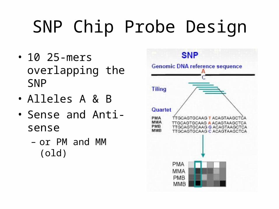
SNP Chip Probe Design
• 10 25-mers overlapping the SNP
• Alleles A & B• Sense and Anti-sense
– or PM and MM (old)

RMA for SNP chips
• Initial Affy software wasn’t very accurate
• Rabbee & Speed (2006) proposed RLMM, an RMA-like method using:– Quantile normalization– Two variables ( A & B signals)– Discriminant analysis
• Much better than Affy software
• Variant (BRLMM) adopted by Affy
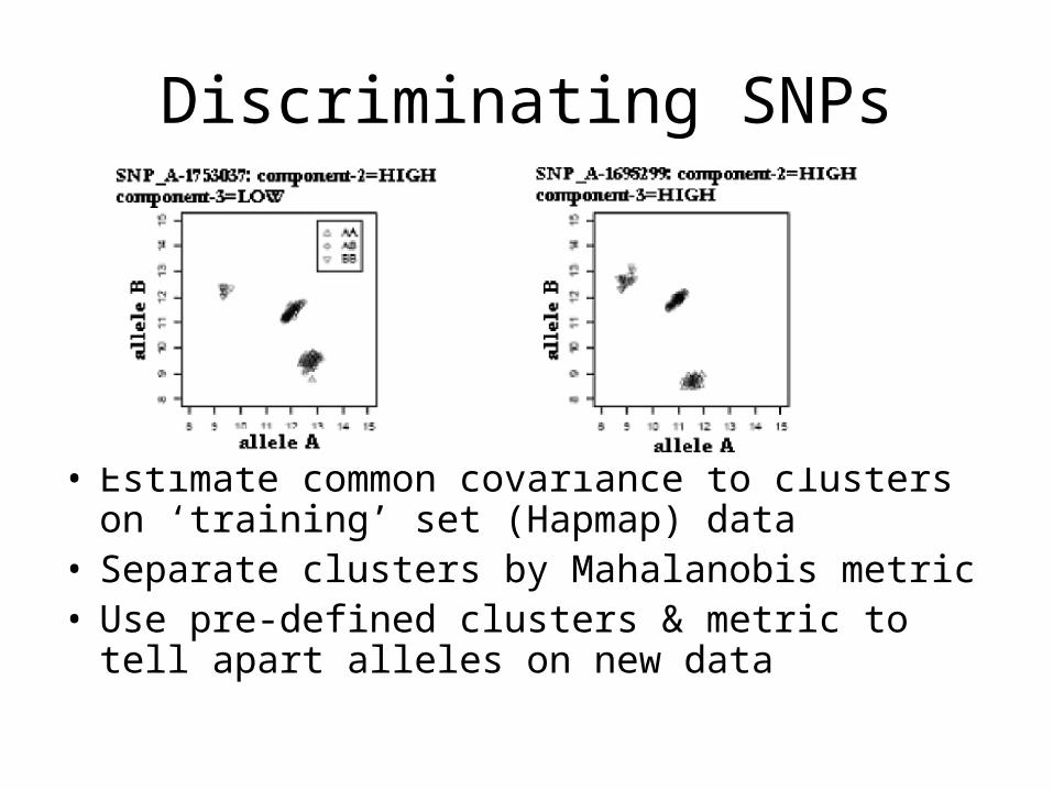
Discriminating SNPs
• Estimate common covariance to clusters on ‘training’ set (Hapmap) data
• Separate clusters by Mahalanobis metric • Use pre-defined clusters & metric to tell apart
alleles on new data
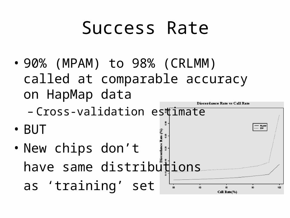
Success Rate
• 90% (MPAM) to 98% (CRLMM) called at comparable accuracy on HapMap data– Cross-validation estimate
• BUT
• New chips don’t
have same distributions
as ‘training’ set

CRLMM - a heroic solution
• RLMM couldn’t be extended across labs
• Still problems with several hundred SNPs
• CRLMM addresses both these issues by careful normalization
• Achieves accuracy of 99.85% on hets; 99.95% on homozygotes
• Most complicated statistical calculation in BioC!

CRLMM Overview
1. Normalize intensity on each chip separately by
2. Summarize ,
, ,
by median polish: M+ =
- ; M- =
-
3. Model log ratio bias on each chip by
4. Estimate log ratio bias using E-M
– Where Zi indexes which SNP state is likely
– k = 1,2,3 for AA, AB, BB
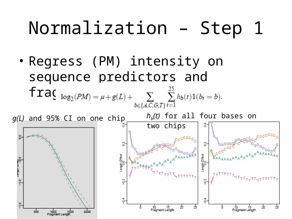
Normalization – Step 1
• Regress (PM) intensity on sequence predictors and fragment length
hb(t) for all four bases on two chipsg(L) and 95% CI on one chip
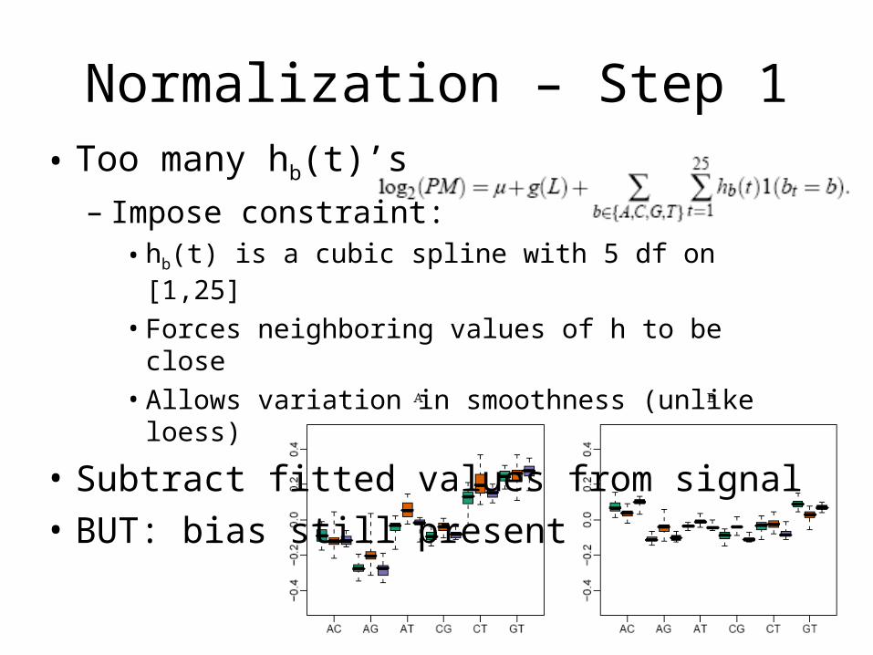
Normalization – Step 1• Too many hb(t)’s
– Impose constraint:• hb(t) is a cubic spline with 5 df on [1,25]
• Forces neighboring values of h to be close• Allows variation in smoothness (unlike loess)
• Subtract fitted values from signal
• BUT: bias still present

Step 2 – Summarization
• Median Polish– Tukey’s exploratory method for arrays of
numbers– Iterative method
• Subtract medians of each row and each column (and accumulate) until medians converge
• Robust
• Fast

Step 3 – Ratio Normalization
• Fit bias function:– of form:
• reflects allele bases
• But what is k?
• Estimate by E-M
fL(L) for one chip

E-M Algorithm
• Systematic way to ‘guess and improve’
• Start with putative assignments to classes– i.e. guess k based on overall separations
• Estimate bias for each k: fi,k• Use residuals from fit to classify again
• Repeat until converge!

Final Step: Calling
• Aim: separation in two-dimensional log-ratio space:
• Accuracy > 99.85% on all Hapmap calls