clustering algorithms for microarray data...
TRANSCRIPT

ISR develops, applies and teaches advanced methodologies of design and analysis to solve complex, hierarchical,heterogeneous and dynamic problems of engineering technology and systems for industry and government.
ISR is a permanent institute of the University of Maryland, within the Glenn L. Martin Institute of Technol-ogy/A. James Clark School of Engineering. It is a National Science Foundation Engineering Research Center.
Web site http://www.isr.umd.edu
I RINSTITUTE FOR SYSTEMS RESEARCH
MASTER'S THESIS
Clustering Algorithms for Microarray Data Mining
by Phanikumar BhamidipatiAdvisor: John S. Baras
MS 2002-4

ABSTRACT
Title of Thesis: CLUSTERING ALGORITHMS FOR MICROARRAY DATA
MINING
Degree Candidate: Phanikumar R. V. Bhamidipati
Degree and year: Master of Science, 2002
Thesis directed by: Professor John S. Baras Department of Electrical and Computer Engineering/Institute for Systems Research
This thesis presents a systems engineering model of modern drug discovery processes and
related systems integration requirements. Some challenging problems include the
integration of public information content with proprietary corporate content, supporting
different types of scientific analyses, and automated analysis tools motivated by diverse
forms of biological data.
To capture the requirements of the discovery system, we identify the processes, users, and
scenarios to form a UML use case model. We then define the object-oriented system
structure and attach behavioral elements. We also look at how object-relational database
extensions can be applied for such analysis.
The next portion of the thesis studies the performance of clustering algorithms based on
LVQ, SVMs, and other machine learning algorithms, to two types of analyses – functional
and phenotypic classification. We found that LVQ initialized with the LBG codebook
yields comparable performance to the optimal separating surfaces generated by related
SVM kernels.
We also describe a novel similarity measure, called the unnormalized symmetric Kullback-
Liebler measure, based on unnormalized expression values. Since the Mercer criterion
cannot be applied to this measure, we compared the performance of this similarity measure
with the log-Euclidean distance in the LVQ algorithm.
The two distance measures perform similarly on cDNA arrays, while the unnormalized
symmetric Kullback-Liebler measure outperforms the log-Euclidean distance on certain
phenotypic classification problems.
Pre-filtering algorithms to find discriminating instances based on PCA, the Find Similar
function, and IB3 were also investigated. The Find Similar method gives the best
performance in terms of multiple criteria.
CLUSTERING ALGORITHMS FOR
MICROARRAY DATA MINING
by
Phanikumar R V Bhamidipati
Thesis submitted to the Faculty of the Graduate School of the University of Maryland, College Park in partial fulfillment
of the requirements for the degree of Master of Science
2002
Advisory Committee
Professor John S. Baras, Chair Associate Professor Mark A. Austin Professor Carlos A. Berenstein


ii
ACKNOWLEDGEMENTS
I would like to express my gratitude to Prof. John S Baras, Lockheed Martin Chair in
Systems Engineering, for his guidance, support, and advice, throughout my thesis research
at the University of Maryland, College Park.
I would also like to thank Automation, Information, and Management Systems (AIMS),
Inc. for the offer of summer internship, their continuous interaction and support with regard
to microarray expression bioinformatics. I appreciate the valuable inputs provided by Dr.
Bernard A Frankpitt of AIMS, Inc. in introducing me to the concepts of microarray data
processing and appropriate software architectures.
I also would like to thank Alexander Baras of Georgetown University and AIMS, Inc., for
explaining the biological details supporting the development and use of microarray data
processing, and for his close collaboration on the biological aspects of the research.
This work was supported by the NSF Combined Research and Curriculum Development
(CRCD) grant (NSF Grant Number: EEC0088112)

iii
TABLE OF CONTENTS
LIST OF TABLES....................................................................................................VI
LIST OF FIGURES................................................................................................VIII
CHAPTER 1: INTRODUCTION ...............................................................................1
1.1 Outline of the Thesis ........................................................................................................ 1
CHAPTER 2: GENETICS AND GENE EXPRESSION............................................3
2.1 DNA Structure and Function ......................................................................................... 3
2.2 Protein Synthesis .............................................................................................................. 5
2.3 Regulation of Gene Expression ...................................................................................... 7 2. 3.1 Chromatin Structure................................................................................................... 8 2.3.2 Transcriptional Control............................................................................................... 8 2. 3.3 Processing-level Control............................................................................................ 9 2.3.4 Translational Control .................................................................................................. 9 2.3.5 Post-translational Factors............................................................................................ 9
CHAPTER 3: GENE EXPRESSION ANALYSIS...................................................11
3.1 Microarray Technology................................................................................................. 11 3.1.1 Oligonucleotide Arrays............................................................................................. 12 3.1.2 cDNA Microarrays ................................................................................................... 13
3.2 Nature of Microarray Data........................................................................................... 15
CHAPTER 4: USE-CASE MODELING OF MICROARRAY ANALYSIS..............18
4.1 Introduction .................................................................................................................... 18
4.2 Overview of Drug Discovery and Development ......................................................... 18 4.2.1 Traditional Drug Discovery...................................................................................... 19 4.2.2 Modern Drug Discovery........................................................................................... 24
4.3 System Description and System Requirements.......................................................... 28
iv
4.4 UML Requirements Modeling...................................................................................... 29 4.4.1 Use Cases Associated with a Biologist .................................................................... 30 4.4.2 Use Cases Associated with a Chemist...................................................................... 32 4.4.3 Use Cases Associated with a Pharmacologist/Toxicologist .................................... 34 4.4.4 Use Cases Associated with a Clinical Scientist ....................................................... 35 4.4.5 Use Cases Associated with a Lab Manager ............................................................. 35 4.4.6 Use Cases Associated with a Product Development Manager................................ 35 4.4.7 Use Cases Associated with a Computational Biologist/Chemist ............................ 36 4.4.8 Use Cases Associated with a Technology Manager ................................................ 37 4.4.9 Use Cases Associated with the System Developer .................................................. 37
4.5 System Structure ............................................................................................................ 41 4.5.1 Package Architecture ................................................................................................ 41 4.5.2 Class Diagrams ......................................................................................................... 44
4.6 System Behavior............................................................................................................. 49
4.7 System Architecture Summary .................................................................................... 56
4.8 Data Architecture and Database Extensions .............................................................. 59
CHAPTER 5: LEARNING ALGORITHMS.............................................................61
5.1 Introduction .................................................................................................................... 61
5.2 Similarity Measures ....................................................................................................... 61 5.2.1 Microarray Expression Data..................................................................................... 61 5.2.2 Probabilistic Models of Microarray Data................................................................. 62 5.2.3 Unnormalized Symmetric Kullback-Liebler Measure............................................. 62
5.3 Learning Algorithms ..................................................................................................... 65 5.3.1 LBG/LVQ Algorithm ............................................................................................... 65 5.3.2 Support Vector Machines ......................................................................................... 68 5.3.2 IB3 Algorithm........................................................................................................... 70
CHAPTER 6: RESULTS ........................................................................................73
6.1 Objectives ........................................................................................................................ 73
6.2 Description of Microarray Data................................................................................... 73 6.2.1 Lymphoma Dataset ................................................................................................... 73 6.2.2 Yeast Data ................................................................................................................. 75 6.2.3 Leukemia Data .......................................................................................................... 77
6.3 Methods ........................................................................................................................... 78 6.3.1 Supervised Classification.......................................................................................... 78

v
6.3.2 Similarity-based Clustering ...................................................................................... 78 6.3.3 Comparison of Algorithms ....................................................................................... 79
6.4 Experiments .................................................................................................................... 79 6.4.1 Lymphoma Data........................................................................................................ 79
6.4.1.1 Binary Classification of Cancerous/Non-cancerous Tissues............................ 80 6.4.1.2 Tissue Type Classification of Cancerous Cells ................................................ 81
6.4.2 Gene Functional Classification from yeast data ...................................................... 82 6.4.3 Cancer Classification and Discovery in Leukemia data .......................................... 86
6.4.3.1 Prefiltering with the IB3 Algorithm.................................................................. 87 6.4.3.2 Pre-filtering with the Relative Distance............................................................ 91 6.4.3.3 Pre-filtering with Principal Components Analysis ........................................... 93 6.4.3.4 Pre-filtering with the Find Similar Method ...................................................... 95 6.4.3.5 Comparison of Find Discriminating Methods .................................................. 97
6.5 Conclusions ..................................................................................................................... 99
vi
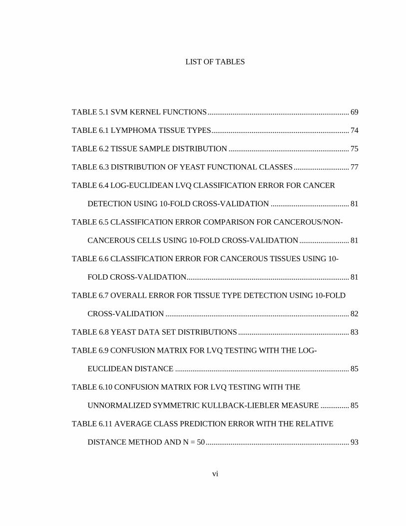
LIST OF TABLES
TABLE 5.1 SVM KERNEL FUNCTIONS.......................................................................... 69
TABLE 6.1 LYMPHOMA TISSUE TYPES........................................................................ 74
TABLE 6.2 TISSUE SAMPLE DISTRIBUTION ............................................................... 75
TABLE 6.3 DISTRIBUTION OF YEAST FUNCTIONAL CLASSES............................. 77
TABLE 6.4 LOG-EUCLIDEAN LVQ CLASSIFICATION ERROR FOR CANCER
DETECTION USING 10-FOLD CROSS-VALIDATION ......................................... 81
TABLE 6.5 CLASSIFICATION ERROR COMPARISON FOR CANCEROUS/NON-
CANCEROUS CELLS USING 10-FOLD CROSS-VALIDATION .......................... 81
TABLE 6.6 CLASSIFICATION ERROR FOR CANCEROUS TISSUES USING 10-
FOLD CROSS-VALIDATION..................................................................................... 81
TABLE 6.7 OVERALL ERROR FOR TISSUE TYPE DETECTION USING 10-FOLD
CROSS-VALIDATION ................................................................................................ 82
TABLE 6.8 YEAST DATA SET DISTRIBUTIONS .......................................................... 83
TABLE 6.9 CONFUSION MATRIX FOR LVQ TESTING WITH THE LOG-
EUCLIDEAN DISTANCE ........................................................................................... 85
TABLE 6.10 CONFUSION MATRIX FOR LVQ TESTING WITH THE
UNNORMALIZED SYMMETRIC KULLBACK-LIEBLER MEASURE ............... 85
TABLE 6.11 AVERAGE CLASS PREDICTION ERROR WITH THE RELATIVE
DISTANCE METHOD AND N = 50 ........................................................................... 93

vii
TABLE 6.12 CLASS DISCOVERY ERROR WITH THE RELATIVE DISTANCE
METHOD....................................................................................................................... 95
viii
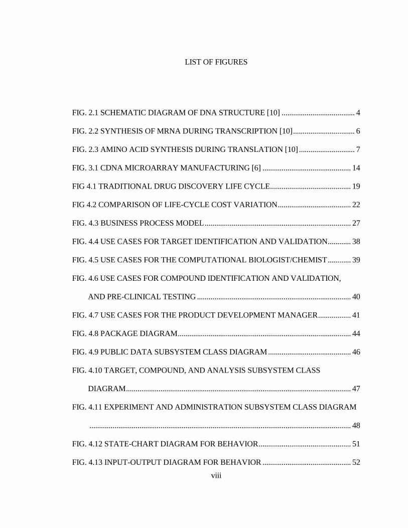
LIST OF FIGURES
FIG. 2.1 SCHEMATIC DIAGRAM OF DNA STRUCTURE [10] ...................................... 4
FIG. 2.2 SYNTHESIS OF MRNA DURING TRANSCRIPTION [10]................................ 6
FIG. 2.3 AMINO ACID SYNTHESIS DURING TRANSLATION [10] ............................. 7
FIG. 3.1 CDNA MICROARRAY MANUFACTURING [6] .............................................. 14
FIG 4.1 TRADITIONAL DRUG DISCOVERY LIFE CYCLE.......................................... 19
FIG 4.2 COMPARISON OF LIFE-CYCLE COST VARIATION...................................... 22
FIG. 4.3 BUSINESS PROCESS MODEL............................................................................ 27
FIG. 4.4 USE CASES FOR TARGET IDENTIFICATION AND VALIDATION............ 38
FIG. 4.5 USE CASES FOR THE COMPUTATIONAL BIOLOGIST/CHEMIST............ 39
FIG. 4.6 USE CASES FOR COMPOUND IDENTIFICATION AND VALIDATION,
AND PRE-CLINICAL TESTING ................................................................................ 40
FIG. 4.7 USE CASES FOR THE PRODUCT DEVELOPMENT MANAGER................. 41
FIG. 4.8 PACKAGE DIAGRAM.......................................................................................... 44
FIG. 4.9 PUBLIC DATA SUBSYSTEM CLASS DIAGRAM........................................... 46
FIG. 4.10 TARGET, COMPOUND, AND ANALYSIS SUBSYSTEM CLASS
DIAGRAM..................................................................................................................... 47
FIG. 4.11 EXPERIMENT AND ADMINISTRATION SUBSYSTEM CLASS DIAGRAM
........................................................................................................................................ 48
FIG. 4.12 STATE-CHART DIAGRAM FOR BEHAVIOR................................................ 51
FIG. 4.13 INPUT-OUTPUT DIAGRAM FOR BEHAVIOR .............................................. 52
ix
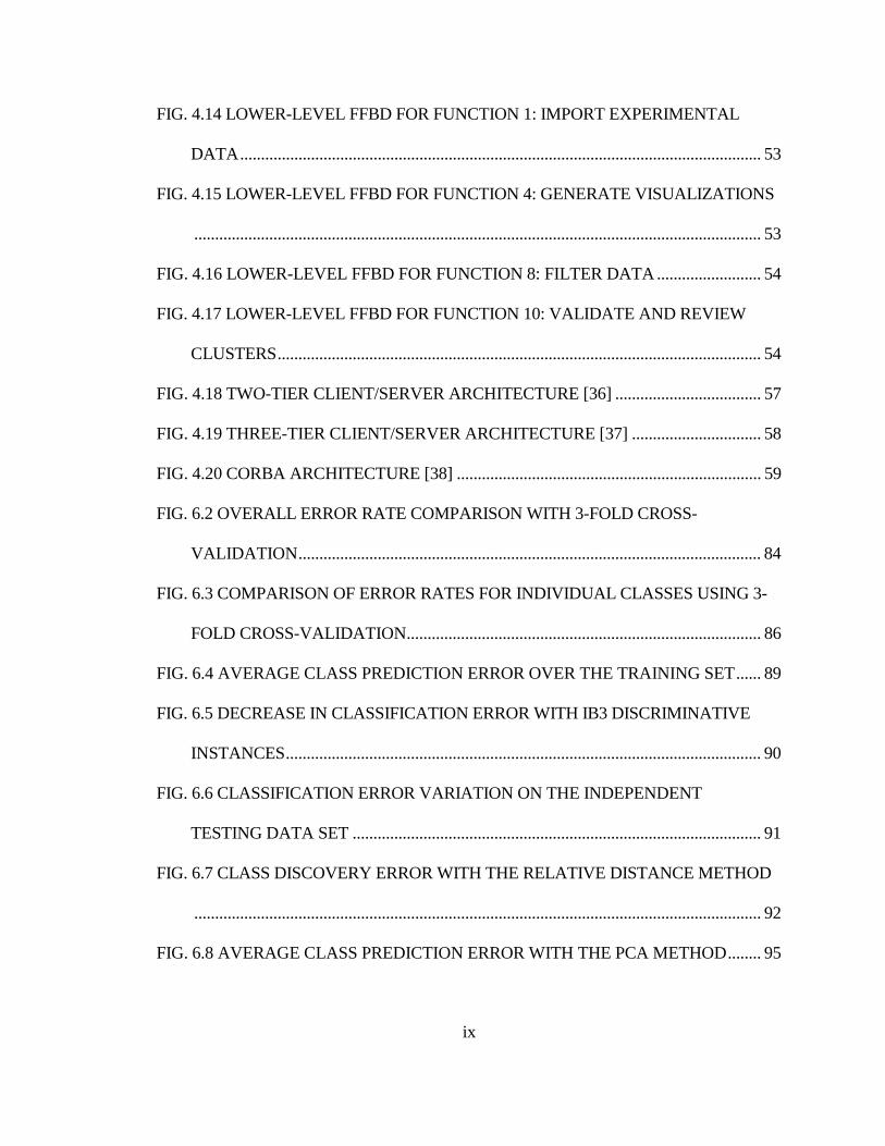
FIG. 4.14 LOWER-LEVEL FFBD FOR FUNCTION 1: IMPORT EXPERIMENTAL
DATA............................................................................................................................. 53
FIG. 4.15 LOWER-LEVEL FFBD FOR FUNCTION 4: GENERATE VISUALIZATIONS
........................................................................................................................................ 53
FIG. 4.16 LOWER-LEVEL FFBD FOR FUNCTION 8: FILTER DATA ......................... 54
FIG. 4.17 LOWER-LEVEL FFBD FOR FUNCTION 10: VALIDATE AND REVIEW
CLUSTERS.................................................................................................................... 54
FIG. 4.18 TWO-TIER CLIENT/SERVER ARCHITECTURE [36] ................................... 57
FIG. 4.19 THREE-TIER CLIENT/SERVER ARCHITECTURE [37] ............................... 58
FIG. 4.20 CORBA ARCHITECTURE [38] ......................................................................... 59
FIG. 6.2 OVERALL ERROR RATE COMPARISON WITH 3-FOLD CROSS-
VALIDATION............................................................................................................... 84
FIG. 6.3 COMPARISON OF ERROR RATES FOR INDIVIDUAL CLASSES USING 3-
FOLD CROSS-VALIDATION..................................................................................... 86
FIG. 6.4 AVERAGE CLASS PREDICTION ERROR OVER THE TRAINING SET...... 89
FIG. 6.5 DECREASE IN CLASSIFICATION ERROR WITH IB3 DISCRIMINATIVE
INSTANCES.................................................................................................................. 90
FIG. 6.6 CLASSIFICATION ERROR VARIATION ON THE INDEPENDENT
TESTING DATA SET .................................................................................................. 91
FIG. 6.7 CLASS DISCOVERY ERROR WITH THE RELATIVE DISTANCE METHOD
........................................................................................................................................ 92
FIG. 6.8 AVERAGE CLASS PREDICTION ERROR WITH THE PCA METHOD........ 95
x
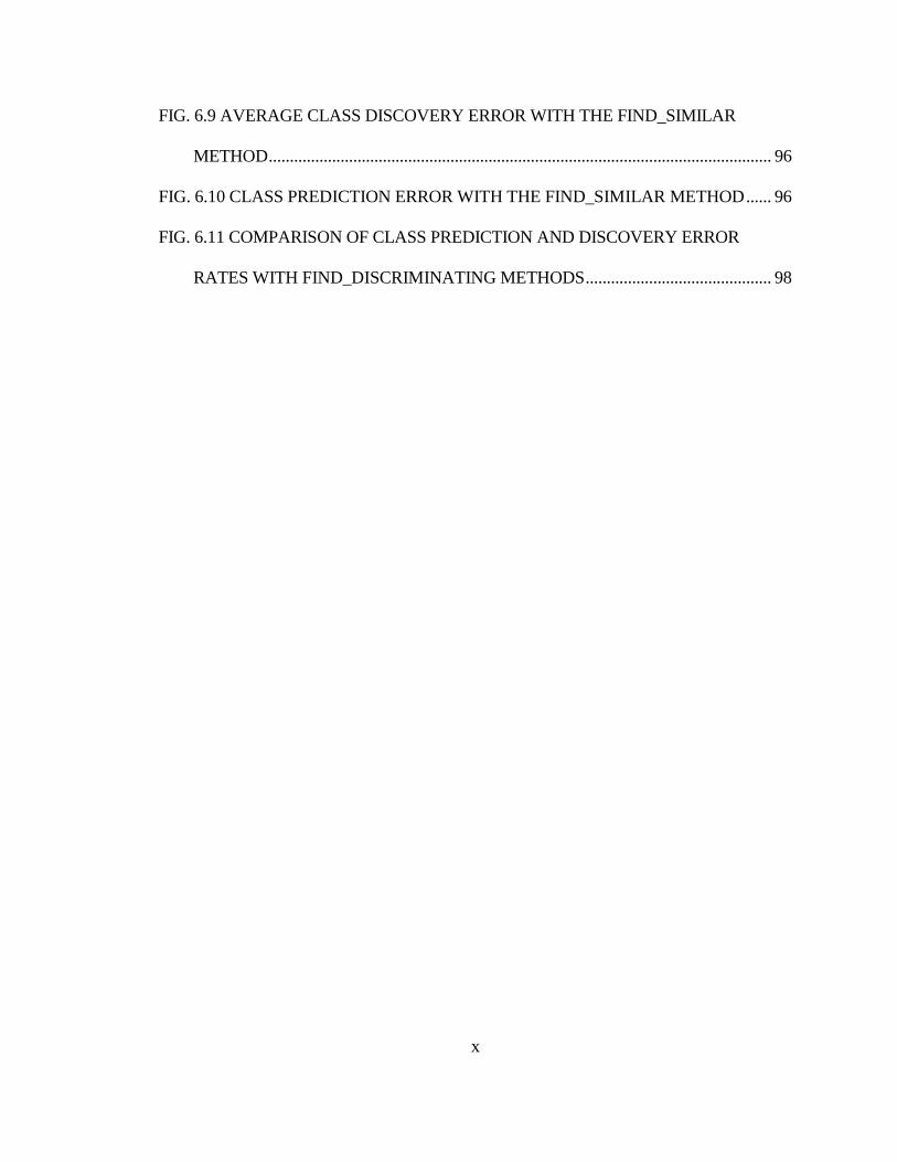
FIG. 6.9 AVERAGE CLASS DISCOVERY ERROR WITH THE FIND_SIMILAR
METHOD....................................................................................................................... 96
FIG. 6.10 CLASS PREDICTION ERROR WITH THE FIND_SIMILAR METHOD...... 96
FIG. 6.11 COMPARISON OF CLASS PREDICTION AND DISCOVERY ERROR
RATES WITH FIND_DISCRIMINATING METHODS............................................ 98
1
CHAPTER 1: INTRODUCTION
1.1 Outline of the Thesis
The thesis is organized as follows.
Chapter 2 gives an overview of genetics and gene expression. It discusses DNA structure
and its role in protein synthesis processes. It also covers representative mechanisms of the
control of gene expression for the interpretation of genetic expression data.
Chapter 3 details large-scale expression analysis using DNA microarrays. Two popular
technologies – oligonucleotide and cDNA arrays, are explained. Based on the overview in
Chapter 2, the nature and analysis of microarray data for gene functional classification are
discussed.
In Chapter 4, we attempt to model the integration of the high-throughput microarray
technology and genetics databases in drug discovery and development processes. We give
a brief overview of traditional and modern drug discovery. UML use cases are developed to
model the requirements of a pharmaceutical discovery/analysis system. The overall system
architecture is described using package and class diagrams, including the behavioral
elements.
Chapter 5 gives an overview of supervised and unsupervised clustering algorithms for
expression analysis. We outline two similarity measures – the log-Euclidean distance and
the unnormalized symmetric Kullback-Liebler measure - and their application in the
(supervised) learning vector quantization (LVQ) algorithm. We also give a brief

2
description of other learning techniques like support vector machines (SVM) and instance-
based learning.
In Chapter 6, we compare different algorithmic implementations of important use cases in
microarray analysis from Chapter 4. Two types of analyses are considered – functional and
phenotypic classification. We give a description of the data sets, the methods and
performance measures used, and a summary of the results.
3
CHAPTER 2: GENETICS AND GENE EXPRESSION
The biological information in an organism is contained in the DNA molecule, which is
present in all cells. Cellular processes such as growth, replication, differentiation, and
response to environmental conditions, are controlled by the DNA sequence data and the
interaction of DNA with cellular compounds.
2.1 DNA Structure and Function
In this section, we elaborate on how the structure of the DNA molecule plays a vital role in
regulating biochemical activities, and discuss mechanisms by which this is carried out.
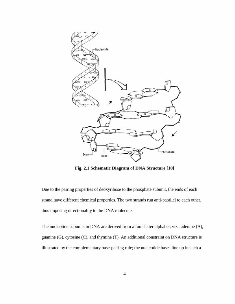
The DNA molecule consists of two strands of nucleotide sequences forming a double-
helical structure. Individual strands are composed of repeating blocks of deoxyribose sugar
and phosphate subunits forming the exterior backbone of the molecule, and a nucleotide
base on the interior. The two strands are held by hydrogen bonding between the nucleotide
bases, as shown in Fig. 2.1.
4
Fig. 2.1 Schematic Diagram of DNA Structure [10]
Due to the pairing properties of deoxyribose to the phosphate subunit, the ends of each
strand have different chemical properties. The two strands run anti-parallel to each other,
thus imposing directionality to the DNA molecule.
The nucleotide subunits in DNA are derived from a four-letter alphabet, viz., adenine (A),
guanine (G), cytosine (C), and thymine (T). An additional constraint on DNA structure is
illustrated by the complementary base-pairing rule; the nucleotide bases line up in such a
5
way that adenine on one strand corresponds to thymine on the other, and guanine
corresponds to cytosine.
2.2 Protein Synthesis
The nucleotide sequences in a DNA molecule act as a template for synthesizing proteins;
enzyme molecules catalyze these reactions. Most of the enzymes are proteins themselves,
with structural properties that render them suitable for specific cellular processes. The order
of reaction events in a cell is determined by a combination of sequence information and the
presence of enzymes.
Sections of the DNA molecule called genes contain the information for synthesizing
specific proteins, which are essentially amino-acid sequences. The information for protein
synthesis is organized in nucleotide triplets called codons, defined by the four-letter DNA
alphabet. Codons act as the template for 20 different amino acids, as well as start and stop
markers for protein synthesis.
Gene expression is the physiological manifestation of the genetic makeup of an organism.
At a finer level, it is the process by which information on a gene is used for protein
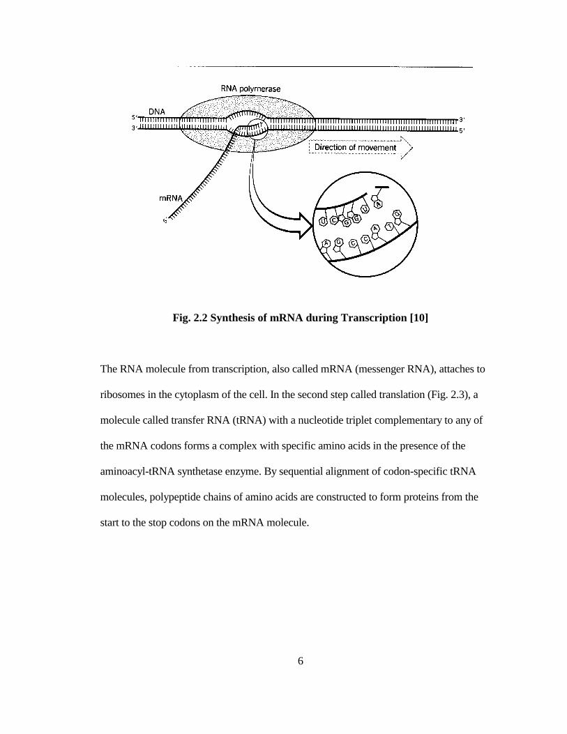
synthesis. It takes place in two steps. During transcription (Fig. 2.2), a single-stranded
ribonucleic acid (RNA) molecule is synthesized based on the complementary genetic
sequence, in the presence of the RNA polymerase enzyme. The RNA molecule is
structurally similar to the DNA molecule and is composed of the four-letter alphabet
AUGC, with uracil (U) in place of the thymine (T) base.
6
Fig. 2.2 Synthesis of mRNA during Transcription [10]
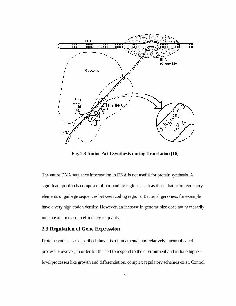
The RNA molecule from transcription, also called mRNA (messenger RNA), attaches to
ribosomes in the cytoplasm of the cell. In the second step called translation (Fig. 2.3), a
molecule called transfer RNA (tRNA) with a nucleotide triplet complementary to any of
the mRNA codons forms a complex with specific amino acids in the presence of the
aminoacyl-tRNA synthetase enzyme. By sequential alignment of codon-specific tRNA
molecules, polypeptide chains of amino acids are constructed to form proteins from the
start to the stop codons on the mRNA molecule.
7
Fig. 2.3 Amino Acid Synthesis during Translation [10]
The entire DNA sequence information in DNA is not useful for protein synthesis. A
significant portion is composed of non-coding regions, such as those that form regulatory
elements or garbage sequences between coding regions. Bacterial genomes, for example
have a very high codon density. However, an increase in genome size does not necessarily
indicate an increase in efficiency or quality.
2.3 Regulation of Gene Expression
Protein synthesis as described above, is a fundamental and relatively uncomplicated
process. However, in order for the cell to respond to the environment and initiate higher-
level processes like growth and differentiation, complex regulatory schemes exist. Control
8
can occur at various stages of the protein synthesis process. In this section, we illustrate a
few well-known mechanisms of gene expression regulation and relate them to gene
function.
2. 3.1 Chromatin Structure
The chromatin is the fibrous complex of DNA and proteins within the nucleus. The
physical structure of the DNA in the chromatin can vary in differentiated cells in an
organism, and result in enhancing or repressing the expression of specific genes. For
instance, the presence of compounds like histones, might affect the ability of RNA
polymerase and transcriptional regulatory proteins to access specific genes on the DNA.
2.3.2 Transcriptional Control
Repression is a transcriptional control mechanism to turn specific genes on or off and is
explained by the operon model of regulation in prokaryotic cells (cells having no nuclear
membrane). The model states that groups of genes coding for related proteins exist close to
each other on the DNA and are controlled by a single promoter region, where the
transcriptional enzyme RNA polymerase attaches itself. The operator region separates the
upstream promoter site from the genes. In the case of the lac operon, the constituent genes
code for enzymes to break down lactose. In the absence of lactose, a regulatory gene
upstream of the promoter codes for a repressor protein that binds to the operator region and
inhibits transcription initiation. When lactose is present, it forms a complex with the
repressor protein and detaches it from the operator site.

9
Attenuation is the mechanism by which the abundance of a protein inhibits its own
transcription. This occurs in genes that code for energy-consuming processes like amino-
acid production.
In activation, the binding of enhancer proteins near promoter and upstream regions of the
DNA enable the RNA polymerase enzyme action, thereby initiating transcription.
2. 3.3 Processing-level Control
This refers to the relation between the coding scheme of genes and proteins. Proteins are
often encoded by members of a multigene family. A multigene family of genes arises by
undergoing modifications during evolution from a single ancestor. Such a set can code for
homologous proteins with similar functions.
2.3.4 Translational Control
Translation of mRNA can be enhanced or suppressed by the amount of the specific protein
in the cell. For instance, iron is stored in the protein ferritin. When iron levels are low in the
cell, a repressor molecule binds to the mRNA for ferritin inhibiting synthesis. When iron
levels in the cell rise, iron binds to the mRNA-repressor complex and detaches the
repressor protein, thereby enhancing the synthesis of ferritin for storage.
2.3.5 Post-translational Factors
Protein expression varies even after translation. The presence of an inhibitor in the
environment can repress protein function. Most proteins exist in an inactive state after
translation and need to undergo polypeptide cleavage to become active. Some proteins may
10
also require activation through a combination with another molecule. The operation of
enzymes in the presence of a cofactor is an example.
Many other mechanisms of gene regulation at various levels of biochemistry exist, and
these may be specific to organisms. However, it is important to note that not all changes are
observable in gene expression experiments. Hence, knowledge of the metabolism,
phylogeny, and careful experimentation is required to draw meaningful results about gene
functional characteristics.
11
CHAPTER 3: GENE EXPRESSION ANALYSIS
Based on the background on gene expression, we give a brief overview of the state-of-the-
art in microarray technology, and two different types of microarrays. We then discuss the
nature and applications of various gene microarray data. In the section on expression
analysis, we explain how microarrays can be related to molecular biology and gene
function.
3.1 Microarray Technology
Genetic analyses have traditionally been based on single-gene experiments in order to
estimate the preferential expression of the gene in multiple experiments. With the
availability of the complete genome sequence information for some organisms, it is now
possible to simulate and study cellular control at the level of genetic interactions. The
DNA microarray is an experimental tool that combines genome information with chip
technology, and allows us to monitor specifically, the gene expression of thousands of
genes at the same time, in different environmental conditions designed by the
investigating biologist.
DNA microarrays give a quantitative measure of gene expression from all genes in a tissue
sample, under a variety of conditions. To explore various genetic properties, experimental
methods need to be designed to map them to expression values.
Microarrays measure the ability of DNA or RNA sequences from a sample to bind (or
hybridize) to their complementary DNA sequences (cDNAs) laid out on a chip. Because of
12
complementary base pairing, measurement of the degree of hybridization between nucleic
acids provides good sensitivity and specificity in detection. This basic idea remaining the
same, two popular techniques exist to measure gene expression on microarrays. They differ
in the manner in which the sequences are prepared initially and are described in the
sections below.
3.1.1 Oligonucleotide Arrays
Oligonucleotides are nucleotide sequences that are 5-25 bases long. The oligonucleotide
array was the first microarray product developed by Affymmetrix. In a procedure similar to
semiconductor manufacturing, it uses photolithography techniques to synthesize nucleotide
sequences.
The entire chip is initially covered with the photolithographic mask. The laser exposes
precise locations on the chip. The particular amino acid solution is passed over the chip and
binds nucleotides at these locations.
The masking agent is applied again and the process is repeated until sequences up to 25
base pairs are generated. Finally, when the fluorescently tagged DNA sequences are treated
with the oligonucleotides, the degree of hybridization is measured by the amount of
fluorescent emission following laser excitation.
A unique feature of oligonucleotide arrays compared to other microarray techniques is their
high degree of accuracy. They hybridize multiple independent oligonucleotides with
different segments of the same RNA. Two sets of (usually) ten probes, called the perfect
match (PM) and mismatch (MM) probe sets, are used with each pair differing in a single

13
base ([7][5]). The MM probes, which act as the control, are supposed to display a much
lower signal compared to the PM probes. This kind of redundancy leads to more accurate
results as averaging and outlier detection can be performed prior to quantitative evaluation.
Since the hybridization process is simple, these arrays have high reproducibility.
To generate oligonucleotide arrays, clearly, we need to know the entire sequence
information of genes and non-coding regions involved in the experiment. However, once
the sequence is known, it can be used in genotypic analysis ([20]). For example,
resequencing known DNA by inserting minor modifications in the complementary
oligonucleotides can detect single nucleotide polymorphisms (SNPs), which are point
mutations in DNA found in a part of the population. Similarly, such mutations can help in
identifying multiple forms of existence of longer sequences by partial matching. Another
advantage of the technique is that since the sequence lengths are small, it is possible to
construct high-density chips monitoring relatively larger number of genes.
However, array synthesis is slow and expensive as it uses a large amount of
photolithographic mask reagent during synthesis. These problems are overcome in cDNA
microarrays discussed below.
3.1.2 cDNA Microarrays
cDNA microarrays were first prepared by the Brown Lab of Stanford University. They
improve upon the oligonucleotide arrays by changing the layout strategy in a fundamental
way. Using purified mRNA transcripts from tissues, the reverse-transcription polymerase
chain reaction (RTPCR) is performed to obtain a large number of gene-specific
14
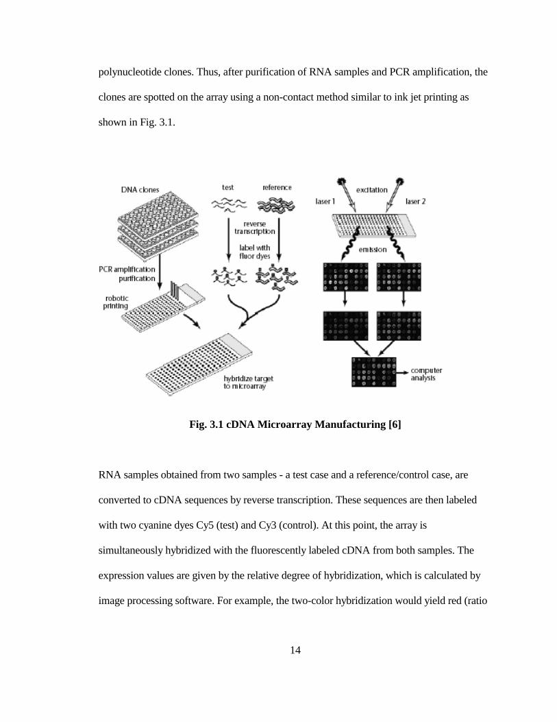
polynucleotide clones. Thus, after purification of RNA samples and PCR amplification, the
clones are spotted on the array using a non-contact method similar to ink jet printing as
shown in Fig. 3.1.
Fig. 3.1 cDNA Microarray Manufacturing [6]
RNA samples obtained from two samples - a test case and a reference/control case, are
converted to cDNA sequences by reverse transcription. These sequences are then labeled
with two cyanine dyes Cy5 (test) and Cy3 (control). At this point, the array is
simultaneously hybridized with the fluorescently labeled cDNA from both samples. The
expression values are given by the relative degree of hybridization, which is calculated by
image processing software. For example, the two-color hybridization would yield red (ratio
15
Cy5/Cy3>1) when the gene is induced, or green when it is repressed, or yellow when there
are no changes.
The cDNA method of fabrication is quick and less expensive compared to oligonucleotide
arrays, and allows the production of oligonucleotides longer than 500 base pairs. The
precise arrangement of spots leads to accurate signal measurement. The individual
expression values are normalized with respect to extracted subsets of closely related
samples.
One chief disadvantage of cDNA microarrays is that it monitors the expression of relatively
fewer genes. Since hybridization ratios are not reliable when gene expression is compared
across chips, this poses an obstacle for large genomes.
Another problem with cDNA microarrays is that they are limited by the availability of
clones for the solid phase and the purity of RNA samples derived from tissues. Further,
cDNA microarrays require a large quantity of RNA (usually 50-200 micrograms) per
hybridization [6].
3.2 Nature of Microarray Data
Since microarray expression data are going to be the basis for gene function prediction in
many applications, we list some of the limitations of microarrays and their role in
experimental design.

16
1. The quality of microarray data depends on its mRNA source. Tissue samples used
in in vivo experiments might be composed of inseparable cell types, and might
show large variability during replication of experiments.
2. With regard to time-series data, it is important to note that individual cycle times of
individual processes have order-of-magnitude differences. Expression analysis can
be used to reveal interactions at the gene-to-gene level but not at the level of
cellular processes/mechanisms. Based on the knowledge of biochemistry of the
experiment, sampling should be carefully designed to enunciate valid and
significant interactions.
a. Unwinding of the helix ~ microseconds
b. Transcription ~ seconds
c. Translation ~ minutes
d. Life of a protein ~ hours
3. A microarray dataset represents a snapshot of particular cell lines. This cell ‘state’
varies significantly based on the environmental conditions, the stage of the cell
cycle, etc. Hence, it is essential to collect multiple data points for each gene and
base inferences on average values.
4. Measurement of mRNA transcript levels after hybridization might not be a true
indicator of protein levels due to post-transcriptional factors (See Sec. 2.3.5). If the
proteins are synthesized, they sometimes might not have any physiological
consequence in the experiment. In such cases, a combination of the knowledge of

17
protein interactions and gene expression values might be a good indicator of gene
function.
18
CHAPTER 4: USE-CASE MODELING OF MICROARRAY
ANALYSIS
4.1 Introduction
In this chapter, firstly, a brief description of processes in pharmaceutical drug development
is given. The impact of the high-throughput microarray technology on processes in
pharmaceutical research and development is explained. A UML systems engineering model
of an analysis system for modern drug development is developed, that captures the high-
level requirements. In the UML use cases, the main actors and their interaction with the
system are studied to build a structural model. From the UML model, we construct a
database schema for microarray data mining. Finally, we look at alternate system and data
architectures for pharmaceutical analysis in an enterprise.
4.2 Overview of Drug Discovery and Development
The discovery and development of drugs involves several stages, and careful planning and
allocation of large investments and time. A drug research plan might attempt to target an
untreated disease, or improve upon an existing drug using a novel approach. The decision
to pursue any project is based on criteria such as the immediate medical requirements, the
effectiveness of current products, etc.
According to the 2000-2001 statistics from Pharmaceutical Research and Manufacturers of
America (PhRMA), for every 5000 medicines tested, 5 of them pass on to undergo clinical
trials, of which only one is accepted ([32]). Considering that the average development cost
19
for a single drug costs $500 million and 12-15 years and the fact that only 30% of marketed
drugs generate revenues in excess of development costs, it is imperative for pharmaceutical
companies to investigate the integration of new genomic technology in dealing with their
lifecycle cost breakdown.
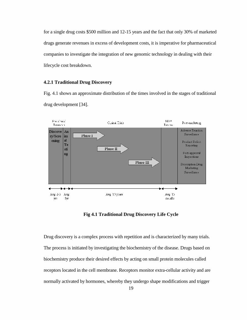
4.2.1 Traditional Drug Discovery
Fig. 4.1 shows an approximate distribution of the times involved in the stages of traditional
drug development [34].
Fig 4.1 Traditional Drug Discovery Life Cycle
Drug discovery is a complex process with repetition and is characterized by many trials.
The process is initiated by investigating the biochemistry of the disease. Drugs based on
biochemistry produce their desired effects by acting on small protein molecules called
receptors located in the cell membrane. Receptors monitor extra-cellular activity and are
normally activated by hormones, whereby they undergo shape modifications and trigger
20
cellular responses. Since receptors are connected with signaling pathways, they are able to
swiftly affect cellular mechanisms by reacting with drug molecules.
The molecular biologist uses biochemical pathways participating in the disease
pathophysiology to form a hypothesis about the chemical reactions involved. Common
drug targets chosen are those that code for enzymes, transporters, and hormone receptors,
since they can be easily controlled by small external molecules.
Feasible lead compounds are selected based on the knowledge of their structure and action.
A majority of these lead compounds arise from natural extracts, which have been
discovered and proven effective previously. The targets are purified and screened against a
variety of lead compounds. The lead compounds are filtered based on their effectiveness on
the drug target. They are then optimized by combinatorial chemistry techniques to form
new compounds with greater specificity. Pre-clinical testing involves in vitro testing on
tissue samples and in vivo testing on animal models (when available) for compound
toxicity. This set of compounds is filtered further to evaluate their side effects, dosage, etc.
on a larger population during the long and expensive clinical trials process.
There are many drawbacks and implicit limitations in the above procedure, in the current
context. The selection of targets is limited by the knowledge of their molecular function.
The proteins that some gene targets encode, like transcription factors, are not easy to
modulate. In the case when the molecular nature of the target is not known, random screens
are performed against thousands of lead compounds, which consume resources, time and
expenses. By having a large number of compounds after screening, the cost of testing is

21
carried over to the expensive development and clinical trials phases. In cases where pre-
clinical testing can be carried out in animal models alone, the same lead compounds might
not be effective in human tissues, as some receptors are very species-specific; this risk is
carried on to the expensive clinical trials process.
Research and pre-clinical testing are the steps where automation and new technology can
play an important role in reducing process times and carry-over costs. The sequencing of
the human genome, miniaturization and automation of key biological processes, high-
throughput techniques like microarrays and the increasing integration of public information
can dramatically reduce the time, risk, and expenses involved in the drug development life
cycle.
Using microarrays, it is possible to screen lead compounds against all known genes and
filter out fewer compounds with greater accuracy and possibility of success. This is
illustrated below in Fig. 4.2 by the percentage expenditure in terms of compound and
development costs involved in these steps.
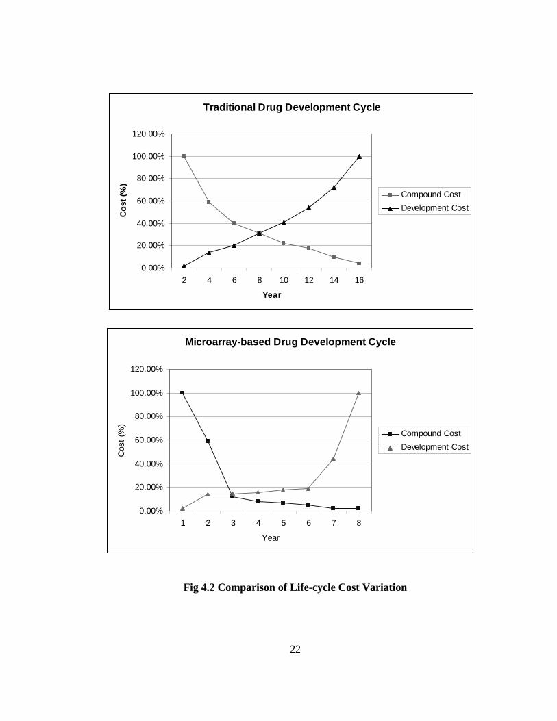
22
Fig 4.2 Comparison of Life-cycle Cost Variation
Traditional Drug Development Cycle
0.00%
20.00%
40.00%
60.00%
80.00%
100.00%
120.00%
2 4 6 8 10 12 14 16
Year
Co
st (
%)
Compound Cost
Development Cost
Microarray-based Drug Development Cycle
0.00%
20.00%
40.00%
60.00%
80.00%
100.00%
120.00%
1 2 3 4 5 6 7 8
Year
Cos
t (%
)
Compound Cost
Development Cost
23
In comparison with Fig. 4.1, the following is an estimate of how micro-array data
processing affects process costs and times for each stage of the life cycle, by bringing down
the number of pre-selected compounds ([33, 35]).
• Research & Pre-clinical Testing: Average 18 months
• Clinical Trials (on human subjects): Average 5 years.
Some examples of the use of new technologies in drug discovery are listed below.
1. Sequence information opens up a large number of new feasible drug targets. It is
possible to conduct genome-wide experiments with microarrays, which have much
lower turnaround times compared to traditional polymerase chain reaction (PCR)
techniques. Gene sequencing from the human genome project is expected to
increase the number of gene targets for drug innovation from 500 to 3000-10000
[8].
2. Diseases like lymphoma and viral infections require drugs that can target the
transcriptional mechanism. Genes related to such cases can be targeted using gene
expression profiling.
3. A single-nucleotide polymorphism (SNP) is a point mutation that represents a
subset of a large population. SNPs are strong markers that can be used in
association studies to identify correlations between the presence of a chromosomal
region and any trait such as a disease phenotype. Microarrays can be used to study
drug response in diverse genotypes in clinical trials.
24
4. Pre-clinical trials can make use of microarrays to conduct toxicology experiments
and to study in vitro testing.
5. Since gene expression is a clear indicator of function, functional prediction of target
genes can lead to rational drug design during the lead identification phase.
6. Gene expression in different experiments and across time points is a fair indication
of gene function. However, in some cases, mRNA levels might not give an
indication of protein levels, due to post-translational factors (Sec. 2.3.5).
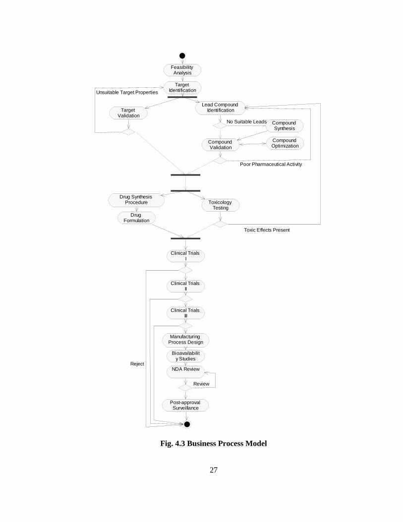
4.2.2 Modern Drug Discovery
Using scenarios of the use of microarrays in modern drug development, a detailed
description of the processes involved in drug discovery is given below. Based on this, the
flow of events is illustrated in the activity diagram of Fig. 4.3.
1. Target Identification and Validation
Target identification is an exploratory phase that involves hypothesizing disease-causing
genes with evidence that can arise from multiple sources. The molecular biologist uses the
knowledge of biochemistry of the disease and associates known targets with new genes of
unknown function through information about DNA sequence, single nucleotide
polymorphisms (SNPs), and population genetics. In cases where little prior knowledge is
available, studies can be based on parallel results from model organisms, or differential
expression profiling of normal and diseased tissues. Information on pathways involving
these targets and sequence homology is also used to suggest alternate genes that can be
attacked.
25
In the target validation step, microarray-based experiments are conducted on the individual
genes to determine their molecular function and interaction with others under different
cellular conditions. They are then filtered by their cellular response and marked as potential
drug targets.
2. Lead Identification and Validation
Biochemical assays of target gene products are developed in a closely similar environment
for in vitro testing. Since the target function may be determined or unknown, they are
screened ‘rationally’ or through random screens against compound library. The compound
library is composed of thousands of synthetic chemicals and natural products.
Cell-based assays, on the other hand, represent animal and cellular models of the disease.
They are used for in vivo testing, and provide more accurate information on drug action
inside the body. While biochemical assays identify lead compounds for a threshold level of
drug action in relevant pathways, cell-based assays also test their potency in being able to
act on cellular models.
These lead compounds are filtered further by studying their specificity, cellular response,
toxicity, and other pharmacological and chemical properties. These validated leads are
characterized by structural properties, which can be found from databases like MDL/ISIS.
Using combinatorial chemistry techniques, they are further optimized by synthesizing lead
compounds with these properties and improved activity on the drug targets.
3. Pre-clinical Testing
26
Pre-clinical testing determines the toxic effects of a particular drug on secondary drug
targets, similar to the lead validation phase. Proteome analysis can be used to determine if
the cell is in a natural state, or showing a specific response mechanism, or an unspecified
response. The subset of proteins showing the response can be analyzed further. These
results can support future characterization of lead compounds during the previous phase.
4. Clinical Trials
In this phase, the drug discovery process is reviewed and clinical trial experiments are
designed to be implemented in the following order.
a. Phase I: Determine potential side effects and dosage of the drug by
administering on 20-80 healthy volunteers.
b. Phase II: Determine effectiveness on a small number of volunteers with the
disease.
c. Phase III: Determine large-scale effectiveness on 1000-3000 patients with
the disease.
d. Regulatory Review and Approval by the FDA.
e. Post-marketing surveillance: Medical practitioners continue to monitor the
drug’s safety and efficacy over a much larger population with the disease.
27
Fig. 4.3 Business Process Model
Feasibility Analysis
Target Identification
Target Validation
Lead Compound Identification
Compound Synthesis
No Suitable Leads
Compound Validation
Compound Optimization
Drug Synthesis Procedure
Drug Formulation
Toxicology Testing
Clinical Trials I
Clinical Trials II
Clinical Trials III
Manufacturing Process Design
Bioavailability Studies
NDA Review
Post-approval Surveillance
Poor Pharmaceutical Activity
Toxic Effects Present
Review
Reject
Unsuitable Target Properties
28
4.3 System Description and System Requirements
A pharmaceutical corporation typically consists of hundreds of users of different
backgrounds such as biologists, chemists, bioinformaticians, clinical scientists, program
managers, and administrators. Users conduct analyses on project-related (transactional)
data such as from experiments, previous analyses, processes, etc. and aggregations of
project data (analytical) at the corporate-level. The applications implementing business
logic are handled by computing on distributed hardware. The broad requirements of an
analysis system within such an enterprise for the modern drug development process can be
listed as follows:
1. Data mining across distributed public and corporate databases.
2. Storage and retrieval of user-specific analyses.
3. Access to archived and current project data such as process status, materials,
analyses, etc. for tracking and prediction in research.
4. (Restricted) Corporate-wide access ability for departmental data stored in a pre-
defined schema/format.
5. Controlled access to different users and customized interfaces for
visualization/data mining.
6. Ability to integrate modules of new functionality with minimal configurational
changes to the system.
7. Database-independent data and results transfer.
29
4.4 UML Requirements Modeling
In this section, we model the high-level requirements of the pharmaceutical analysis system
with UML use cases. These use cases represent unit-transaction scenarios where the users
(actors) interact with system components during different phases of the drug development
life cycle. Knowing the nature of these interactions allows us to create the system structure
in terms of the data model for database system design. This process is an iterative one,
where the structure is related back to the initial requirements model and modified if any
conditions are ambiguous or not met.
The following use cases attempt to model the requirements of a pharmaceutical corporation
in terms of microarray data processing as rigorously as possible. However, when we derive
the class structure from the UML model, some schema elements such as lead compound
properties, storage of results from different public databases, and so on are deliberately left
‘masked’ or undetermined to keep the implementation from becoming too specific while
keeping the model as accurate as possible.
The main actors of the model include the product development manager, computational
biologist/chemists, molecular biologists, pharmacologists, chemists, clinical scientists,
technical managers, system developers, and lab managers. They relate to the drug
development processes that are shown in Fig. 4.3. The use cases are grouped by the users
involved in these major processes. Entities like the corporate knowledge base, public
databases, and transactional databases in the use cases denote subsystems, and are denoted
as actors and abstract entities themselves. They have a detailed structure for different
phases of the process, which will be derived in Section 4.5 on system structure.
30
4.4.1 Use Cases Associated with a Biologist
4.4.1.1 FORMULATE TARGET HYPOTHESIS: This use case deals with the
biologist’s research on feasible targets and results reported to the transactional database.
The biologist queries public databases and the corporate knowledge base about the
biochemistry of the disease. The system collates information and returns the pathways
involved, disease categories, and related targets (genes, receptors, enzymes, and other
proteins). It also retrieves experimental data from normal and diseased cells, and
treatments with several compounds, references, and so on. The biologist stores the
results of the search, including the target, its type, associated diseases, and pathways
involved, in the transactional database.
4.4.1.2 IDENTIFY AND VALIDATE TARGET GENES: The use case provides
shared behavior for the specific use cases such as Find Similar, Find Discriminating,
Pre-filter and Cluster, and Search. It reports the results of experimental findings on
genes from (4.4.1.1) to the transactional database.
With the leads from (4.4.1.1), namely genes involved and corresponding experimental
data, the biologist performs different kinds of analyses. The biologist also specifies
experimental protocols to obtain differential expression data on the activity of the
feasible targets in normal and disease cells. The system retrieves analysis results based
on the criteria and receives analysis reports about the resultant set of genes,
experiments analyzed, similarity measure used, feature analyzed, threshold similarity
(if applicable), and data values used (raw values, normalized logarithmic values, and so
on)
31
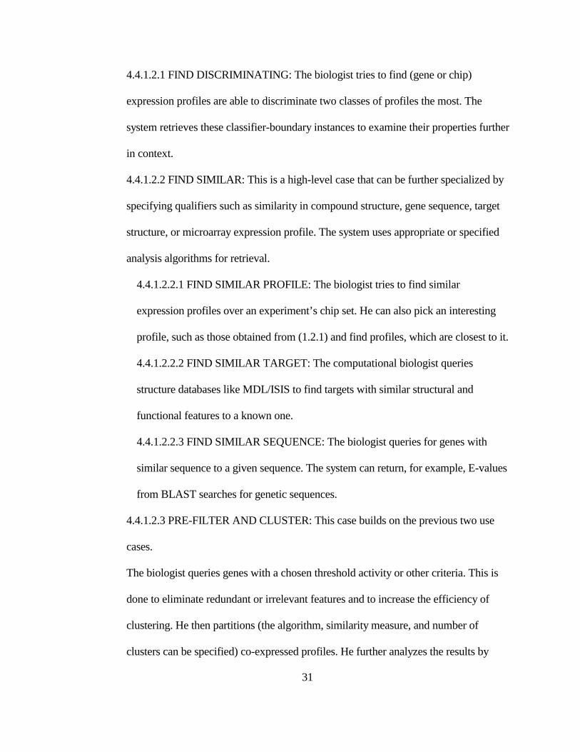
4.4.1.2.1 FIND DISCRIMINATING: The biologist tries to find (gene or chip)
expression profiles are able to discriminate two classes of profiles the most. The
system retrieves these classifier-boundary instances to examine their properties further
in context.
4.4.1.2.2 FIND SIMILAR: This is a high-level case that can be further specialized by
specifying qualifiers such as similarity in compound structure, gene sequence, target
structure, or microarray expression profile. The system uses appropriate or specified
analysis algorithms for retrieval.
4.4.1.2.2.1 FIND SIMILAR PROFILE: The biologist tries to find similar
expression profiles over an experiment’s chip set. He can also pick an interesting
profile, such as those obtained from (1.2.1) and find profiles, which are closest to it.
4.4.1.2.2.2 FIND SIMILAR TARGET: The computational biologist queries
structure databases like MDL/ISIS to find targets with similar structural and
functional features to a known one.
4.4.1.2.2.3 FIND SIMILAR SEQUENCE: The biologist queries for genes with
similar sequence to a given sequence. The system can return, for example, E-values
from BLAST searches for genetic sequences.
4.4.1.2.3 PRE-FILTER AND CLUSTER: This case builds on the previous two use
cases.
The biologist queries genes with a chosen threshold activity or other criteria. This is
done to eliminate redundant or irrelevant features and to increase the efficiency of
clustering. He then partitions (the algorithm, similarity measure, and number of
clusters can be specified) co-expressed profiles. He further analyzes the results by
32
clustering over genes or chip profiles. The system executes server-side algorithms,
retrieves the results, and displays them in a visualization tool.
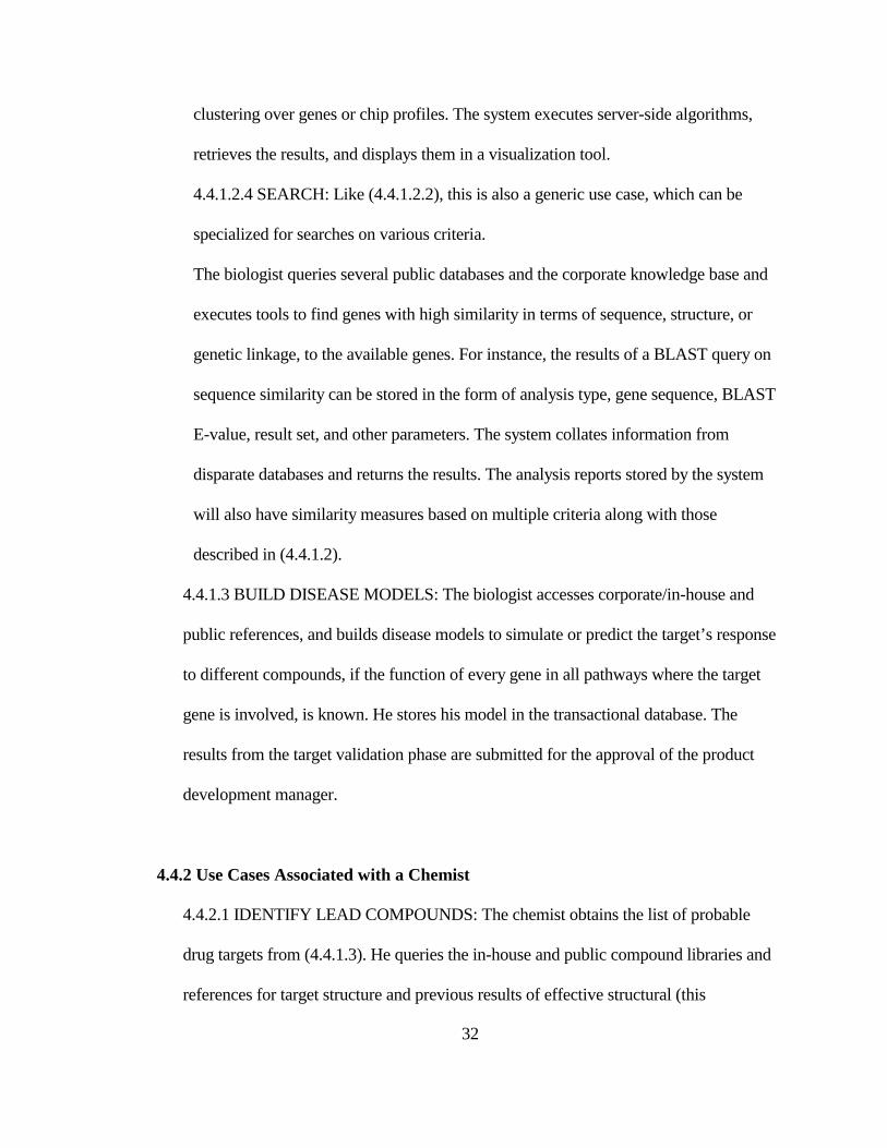
4.4.1.2.4 SEARCH: Like (4.4.1.2.2), this is also a generic use case, which can be
specialized for searches on various criteria.
The biologist queries several public databases and the corporate knowledge base and
executes tools to find genes with high similarity in terms of sequence, structure, or
genetic linkage, to the available genes. For instance, the results of a BLAST query on
sequence similarity can be stored in the form of analysis type, gene sequence, BLAST
E-value, result set, and other parameters. The system collates information from
disparate databases and returns the results. The analysis reports stored by the system
will also have similarity measures based on multiple criteria along with those
described in (4.4.1.2).
4.4.1.3 BUILD DISEASE MODELS: The biologist accesses corporate/in-house and
public references, and builds disease models to simulate or predict the target’s response
to different compounds, if the function of every gene in all pathways where the target
gene is involved, is known. He stores his model in the transactional database. The
results from the target validation phase are submitted for the approval of the product
development manager.
4.4.2 Use Cases Associated with a Chemist
4.4.2.1 IDENTIFY LEAD COMPOUNDS: The chemist obtains the list of probable
drug targets from (4.4.1.3). He queries the in-house and public compound libraries and
references for target structure and previous results of effective structural (this
33
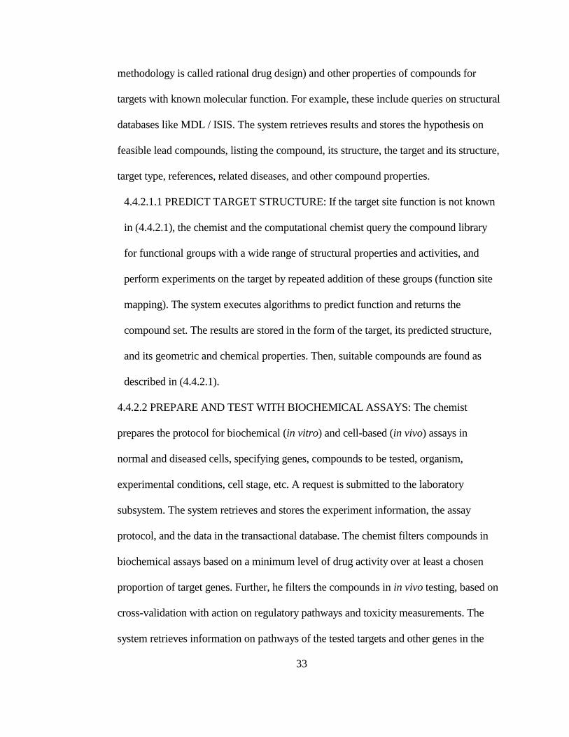
methodology is called rational drug design) and other properties of compounds for
targets with known molecular function. For example, these include queries on structural
databases like MDL / ISIS. The system retrieves results and stores the hypothesis on
feasible lead compounds, listing the compound, its structure, the target and its structure,
target type, references, related diseases, and other compound properties.
4.4.2.1.1 PREDICT TARGET STRUCTURE: If the target site function is not known
in (4.4.2.1), the chemist and the computational chemist query the compound library
for functional groups with a wide range of structural properties and activities, and
perform experiments on the target by repeated addition of these groups (function site
mapping). The system executes algorithms to predict function and returns the
compound set. The results are stored in the form of the target, its predicted structure,
and its geometric and chemical properties. Then, suitable compounds are found as
described in (4.4.2.1).
4.4.2.2 PREPARE AND TEST WITH BIOCHEMICAL ASSAYS: The chemist
prepares the protocol for biochemical (in vitro) and cell-based (in vivo) assays in
normal and diseased cells, specifying genes, compounds to be tested, organism,
experimental conditions, cell stage, etc. A request is submitted to the laboratory
subsystem. The system retrieves and stores the experiment information, the assay
protocol, and the data in the transactional database. The chemist filters compounds in
biochemical assays based on a minimum level of drug activity over at least a chosen
proportion of target genes. Further, he filters the compounds in in vivo testing, based on
cross-validation with action on regulatory pathways and toxicity measurements. The
system retrieves information on pathways of the tested targets and other genes in the
34
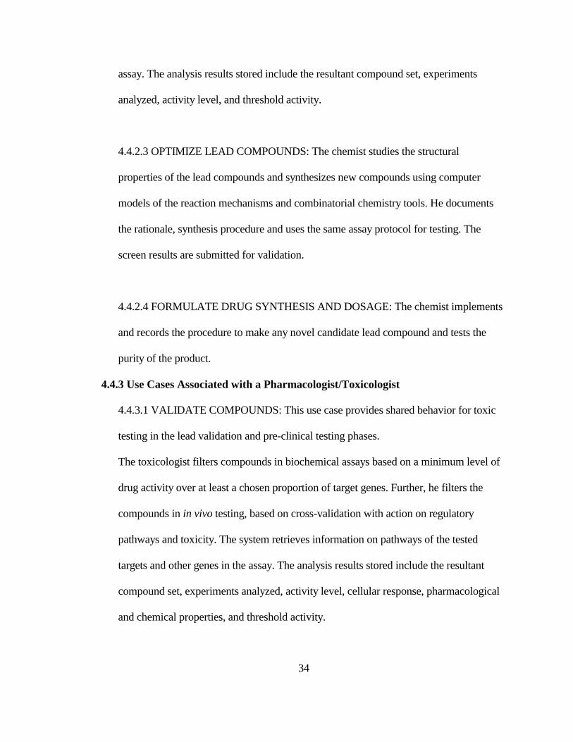
assay. The analysis results stored include the resultant compound set, experiments
analyzed, activity level, and threshold activity.
4.4.2.3 OPTIMIZE LEAD COMPOUNDS: The chemist studies the structural
properties of the lead compounds and synthesizes new compounds using computer
models of the reaction mechanisms and combinatorial chemistry tools. He documents
the rationale, synthesis procedure and uses the same assay protocol for testing. The
screen results are submitted for validation.
4.4.2.4 FORMULATE DRUG SYNTHESIS AND DOSAGE: The chemist implements
and records the procedure to make any novel candidate lead compound and tests the
purity of the product.
4.4.3 Use Cases Associated with a Pharmacologist/Toxicologist
4.4.3.1 VALIDATE COMPOUNDS: This use case provides shared behavior for toxic
testing in the lead validation and pre-clinical testing phases.
The toxicologist filters compounds in biochemical assays based on a minimum level of
drug activity over at least a chosen proportion of target genes. Further, he filters the
compounds in in vivo testing, based on cross-validation with action on regulatory
pathways and toxicity. The system retrieves information on pathways of the tested
targets and other genes in the assay. The analysis results stored include the resultant
compound set, experiments analyzed, activity level, cellular response, pharmacological
and chemical properties, and threshold activity.

35
4.4.3.2 DETERMINE TOXIC EFFECTS: The pharmacologist and toxicologist
perform toxic studies on primary and secondary drug targets as described in (4.4.2.3)
on animal cells. They query proteome information to determine the nature of cell state.
They document characteristics such as cellular response and drug selectivity, potency,
and toxicity.
4.4.4 Use Cases Associated with a Clinical Scientist
4.4.4.1 DETERMINE STUDY PARAMETERS: In the clinical trials phase, the clinical
scientist determines parameters for drug experimentation such as normal dose ranges,
expected values, measurement techniques, and equipment required.
4.4.4.2 DEVISE EXPERIMENTAL PROTOCOL: The scientist prepares a case report
form to study the drug effects on patients, prepares schedules, dosage, etc.
4.4.5 Use Cases Associated with a Lab Manager
4.4.5.1 IMPLEMENT EXPERIMENT PROTOCOLS: The lab technician obtains the
experimental protocol for microarray and assay development from the drug discovery
team. He co-ordinates and documents procedures for sample preparation, hybridization,
normalization, quality check, etc. using a LIMS (Laboratory Information Management
System) tool. The system stores the raw experimental data in the transactional database.
4.4.6 Use Cases Associated with a Product Development Manager
The Product Development Manager oversees the progress of different project groups
working in the firm.
4.4.6.1 CONDUCT FEASIBILITY ANALYSIS: The manager picks a preliminary
research area based on the current demand, knowledge of competing brands, etc. He
queries the corporate knowledge base for availability and potential of compounds in the
36
company’s compound libraries for new products, and the performance and viability of
similar projects. He then initiates a research project. The system collates information
across projects, analysis results, financial and other corporate data for business
decisions.
4.4.6.2 ALLOCATE RESOURCES FOR PROJECTS: With simultaneous drug
development projects in progress, the manager allocates personnel to specific project
phases. He makes decisions on manufacturing or purchasing resources such as
chemical compounds, assays, etc.
4.4.6.3 MONITOR THE PERFORMANCE OF PROJECT GROUPS: On the basis of
the performance of ongoing and past projects, the manager can allow or revoke the
continuation of a particular project phase. For instance, this might be in the form of the
following queries: ‘Which projects have been more productive in terms of the number
of leads?’
4.4.6.4 CONDUCT PEER REVIEW: The peer review team, involving the product
manager, reviews the analyses results at different checkpoints during the drug
discovery life cycle. They approve the transfer of new results at the end of individual
sub phases into the corporate database, and allow other research teams to make use of
these results.
4.4.7 Use Cases Associated with a Computational Biologist/Chemist
4.4.7.1 FIND SIMILAR:
4.4.7.1.1 FIND SIMILAR TARGET: (As in 4.4.1.2.2.2)
4.4.7.1.2 FIND SIMILAR COMPOUND: The computational chemist tries to find
compounds with similar activity and physical properties to a compound known to
37
produce desired therapeutic response on a given target. He performs a large number of
experiments with a wide variety of compound chemistries. The system runs
correlation methods like QSAR (Quantitative Structure Activity Relationship) and
stores the results in the form of the target, the compound, its QSAR activity score, and
its structure.
4.4.7.2 PREDICT TARGET STRUCTURE: (As described in (4.4.2.1.1))
4.4.7.3 DESIGN LIBRARIES: The computational chemist uses combinatorial
chemistry techniques to determine compounds with high activity scores on a chosen
target. The results obtained are similar to (4.4.7.1.2)
4.4.7.4 PREDICT COMPOUND PROPERTIES: (Similar to 4.4.7.1.2) The system runs
correlation methods like QSPR (Quantitative Structure Property Relationship) to
predict the chemical properties given the compound structure.
4.4.8 Use Cases Associated with a Technology Manager
4.4.8.1 ORGANIZE REQUIREMENTS: The technology manager represents the
domain experts from different areas of research and testing in the corporation. He
studies new technology and current shortcomings in the system, and prioritizes new
requirements from different users. He communicates with the system developer to
assess and improve the structure and functionality of the system.
4.4.9 Use Cases Associated with the System Developer
4.4.9.1 OBTAIN REQUIREMENTS: The developer obtains requirements from the
technology manager, and interacts with him to understand how the system will be used.
Changes to the system are to be made incrementally, after new requirements come in.
38
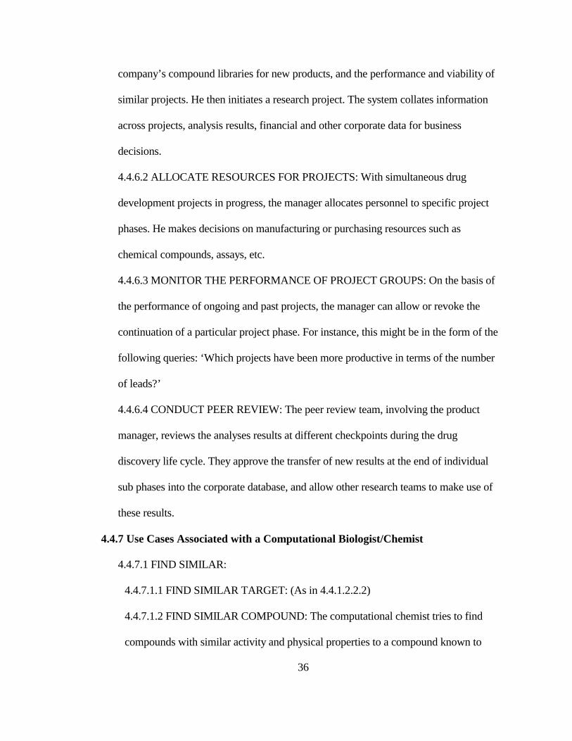
4.4.9.2 DESIGN KNOWLEDGE BASE: The developer designs the database to
organize current as well as archived data and results. He creates a client-server model
of microarray analysis, and designs the interfaces for different users.
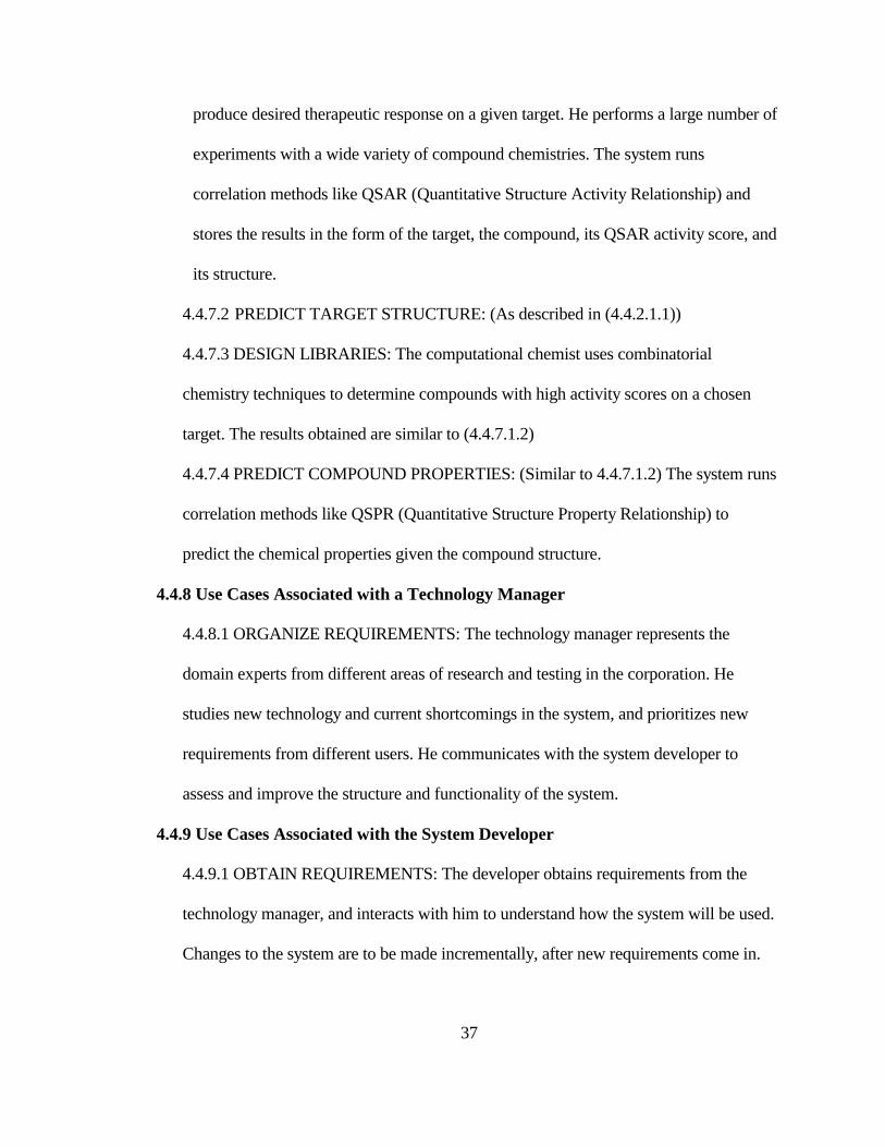
Fig. 4.4 Use Cases for Target Identification and Validation
Pre-fi lter and Cluster
Find Similar Sequence Find Similar Target Find Similar Profi le Find Similar Compound
Identify and Validate Targets
<<Uses>>
Build Disease Models
Biologist Transactional DB
Public DB
Formulate Target Hypothesis Search
<<Uses>>
Find Similar
<<Uses>>
Find Discriminating
<<Uses>>
Corporate KB
<<Extends>>
<<Extends>><<Extends>>
<<Extends>>
39
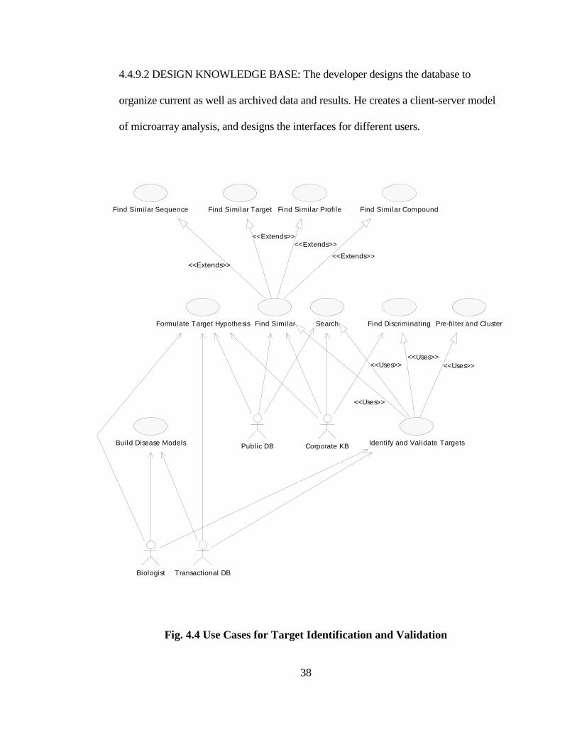
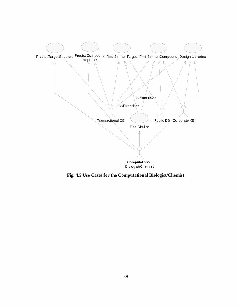
Fig. 4.5 Use Cases for the Computational Biologist/Chemist
Find Similar
Predict Target Structure Predict Compound Properties
Computational Biologist/Chemist
Transactional DB Corporate KB
Find Similar Target
<<Extends>>
Find Similar Compound
<<Extends>>
Design Libraries
Public DB
40
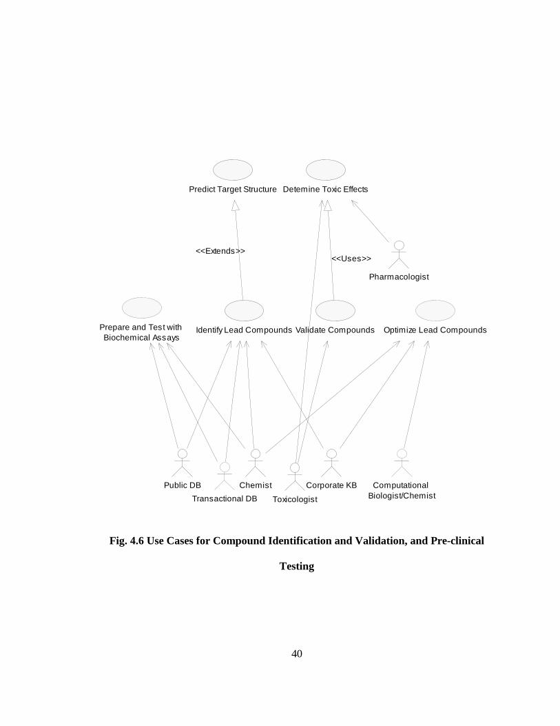
Fig. 4.6 Use Cases for Compound Identification and Validation, and Pre-clinical
Testing
Predict Target Structure
Pharmacologist
Validate Compounds
Detemine Toxic Effects
<<Uses>>
Toxicologist
Public DB
Transactional DB
Prepare and Test with Biochemical Assays
Identify Lead Compounds
<<Extends>>
Chemist Corporate KB
Optimize Lead Compounds
Computational Biologist/Chemist
41
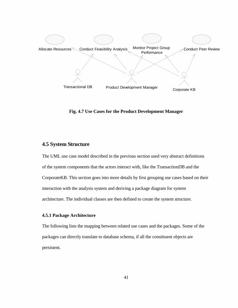
Fig. 4.7 Use Cases for the Product Development Manager
4.5 System Structure
The UML use case model described in the previous section used very abstract definitions
of the system components that the actors interact with, like the TransactionDB and the
CorporateKB. This section goes into more details by first grouping use cases based on their
interaction with the analysis system and deriving a package diagram for system
architecture. The individual classes are then defined to create the system structure.
4.5.1 Package Architecture
The following lists the mapping between related use cases and the packages. Some of the
packages can directly translate to database schema, if all the constituent objects are
persistent.
Allocate Resources
Transactional DB Product Development Manager
Conduct Feasibility Analysis Monitor Project Group Performance
Conduct Peer Review
Corporate KB
42
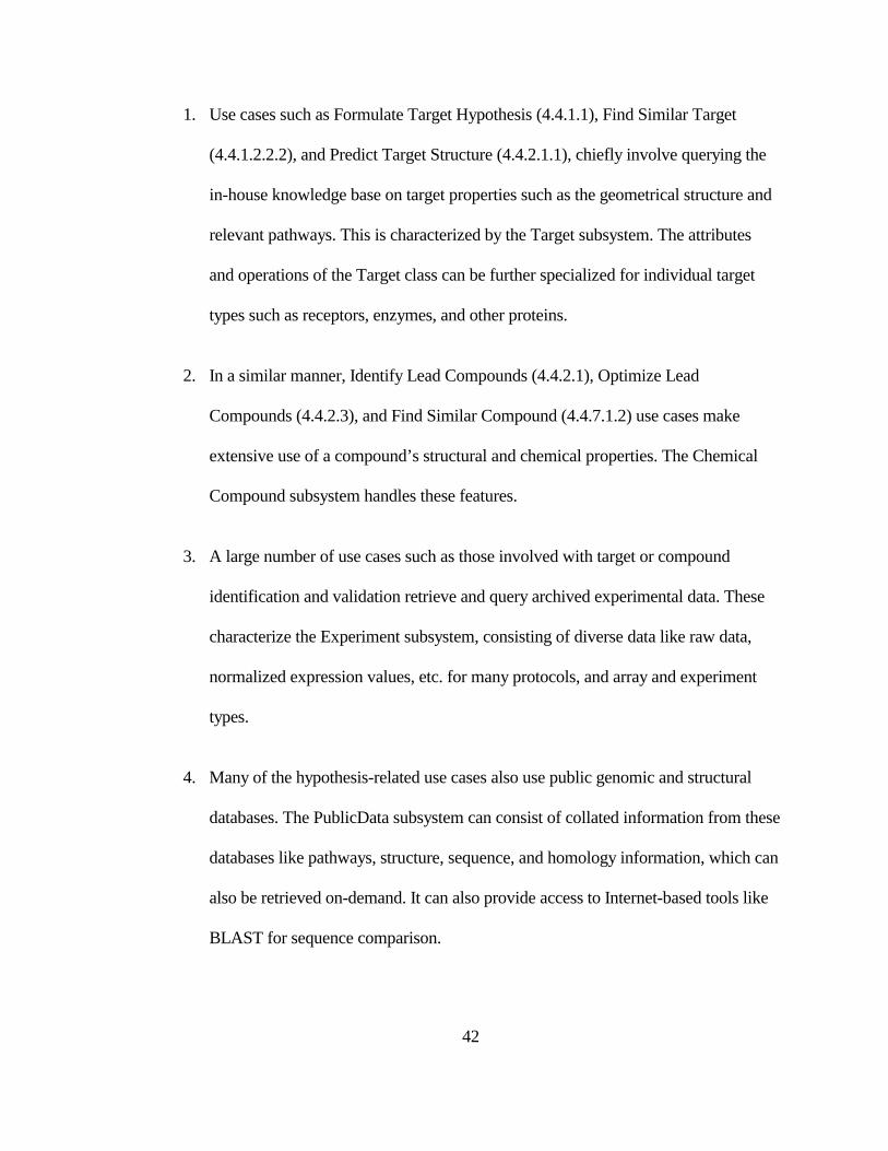
1. Use cases such as Formulate Target Hypothesis (4.4.1.1), Find Similar Target
(4.4.1.2.2.2), and Predict Target Structure (4.4.2.1.1), chiefly involve querying the
in-house knowledge base on target properties such as the geometrical structure and
relevant pathways. This is characterized by the Target subsystem. The attributes
and operations of the Target class can be further specialized for individual target
types such as receptors, enzymes, and other proteins.
2. In a similar manner, Identify Lead Compounds (4.4.2.1), Optimize Lead
Compounds (4.4.2.3), and Find Similar Compound (4.4.7.1.2) use cases make
extensive use of a compound’s structural and chemical properties. The Chemical
Compound subsystem handles these features.
3. A large number of use cases such as those involved with target or compound
identification and validation retrieve and query archived experimental data. These
characterize the Experiment subsystem, consisting of diverse data like raw data,
normalized expression values, etc. for many protocols, and array and experiment
types.
4. Many of the hypothesis-related use cases also use public genomic and structural
databases. The PublicData subsystem can consist of collated information from these
databases like pathways, structure, sequence, and homology information, which can
also be retrieved on-demand. It can also provide access to Internet-based tools like
BLAST for sequence comparison.

43
5. Frequent upgrades of the public databases, archiving validated information or
completed projects, as well as access control privileges and maintenance is handled
by the DB Administration subsystem.
6. The LIMS subsystem deals with laboratory techniques and protocols in the
acquisition and preparation of diverse samples, assays, and microarrays.
7. Finally, the documentation of analysis steps and results from use cases in the target
and lead compound identification and validation phases, are stored in the Analysis
subsystem. This might also consist of archived results from use cases like Predict
Target Structure (4.4.7.2), Design Libraries (4.4.7.3), Predict Compound Properties
(4.4.7.4), Conduct Feasibility Analysis (4.4.6.1), and so on. The storage of data in
this subsystem can be similar to a data warehouse and is used by all the major users
of the system, making it the most important component of the system. It may be
further specialized for target and compound analyses.
Fig. 4.8 shows the high-level package diagram for the analysis system. The arrows indicate
the dependency of packages on each other. The following section discusses the individual
classes in each subsystem.
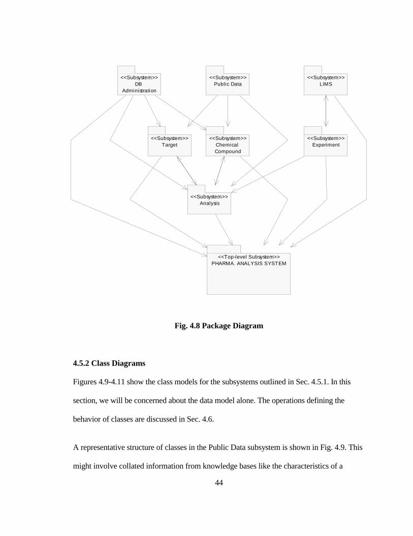
44
Fig. 4.8 Package Diagram
4.5.2 Class Diagrams
Figures 4.9-4.11 show the class models for the subsystems outlined in Sec. 4.5.1. In this
section, we will be concerned about the data model alone. The operations defining the
behavior of classes are discussed in Sec. 4.6.
A representative structure of classes in the Public Data subsystem is shown in Fig. 4.9. This
might involve collated information from knowledge bases like the characteristics of a
PHARMA. ANALYSIS SYSTEM<<Top-level Subsystem>>
Target<<Subsystem>>
Chemical Compound
<<Subsystem>>
DB Administration
<<Subsystem>>
Analysis<<Subsystem>>
LIMS<<Subsystem>>
Public Data<<Subsystem>>
Experiment<<Subsystem>>
45
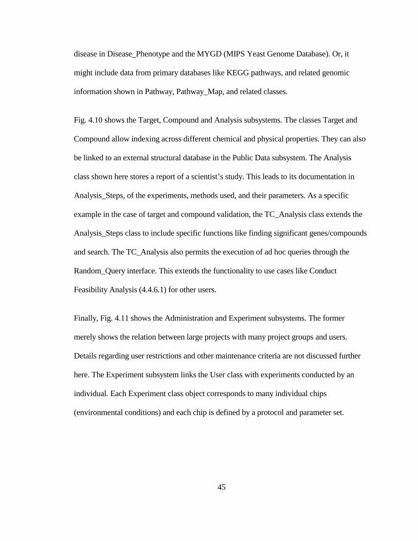
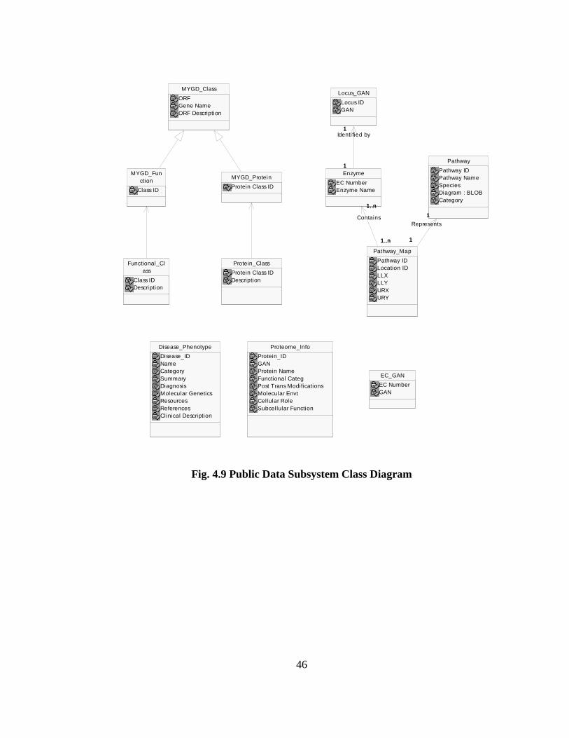
disease in Disease_Phenotype and the MYGD (MIPS Yeast Genome Database). Or, it
might include data from primary databases like KEGG pathways, and related genomic
information shown in Pathway, Pathway_Map, and related classes.
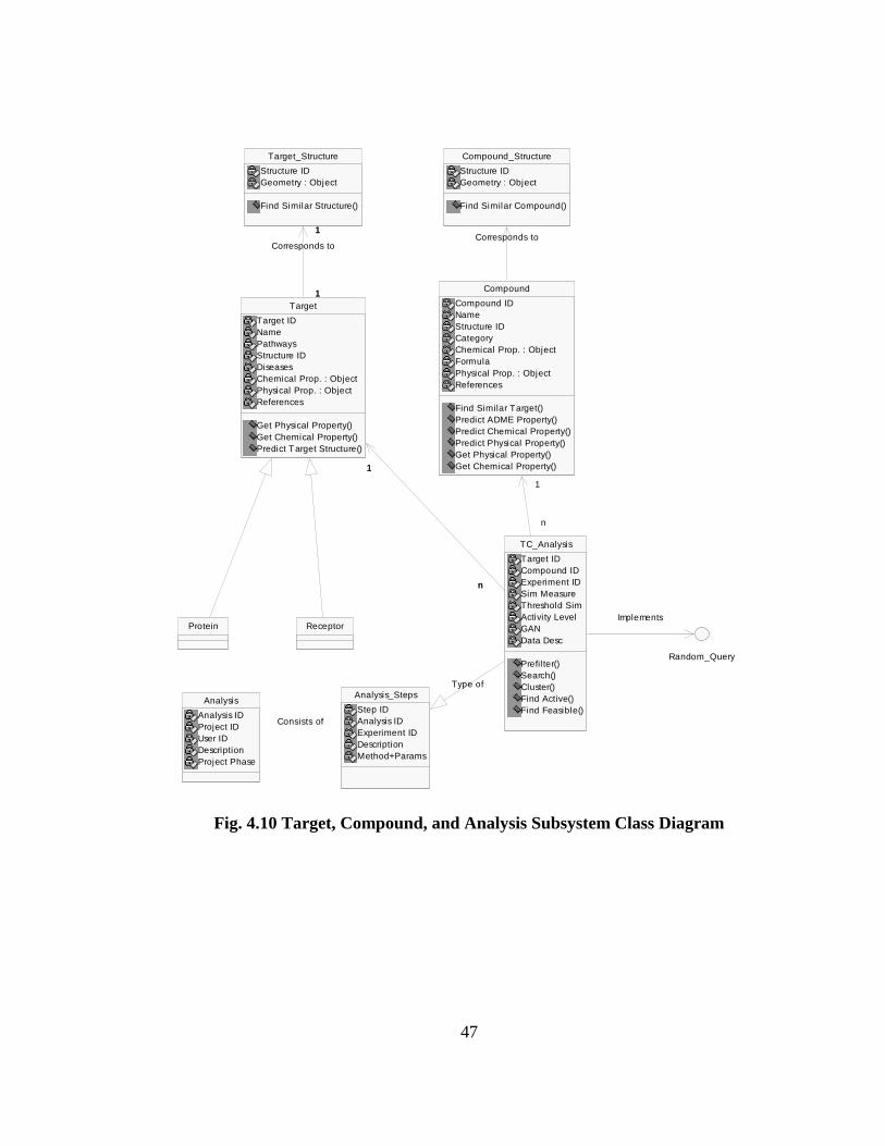
Fig. 4.10 shows the Target, Compound and Analysis subsystems. The classes Target and
Compound allow indexing across different chemical and physical properties. They can also
be linked to an external structural database in the Public Data subsystem. The Analysis
class shown here stores a report of a scientist’s study. This leads to its documentation in
Analysis_Steps, of the experiments, methods used, and their parameters. As a specific
example in the case of target and compound validation, the TC_Analysis class extends the
Analysis_Steps class to include specific functions like finding significant genes/compounds
and search. The TC_Analysis also permits the execution of ad hoc queries through the
Random_Query interface. This extends the functionality to use cases like Conduct
Feasibility Analysis (4.4.6.1) for other users.
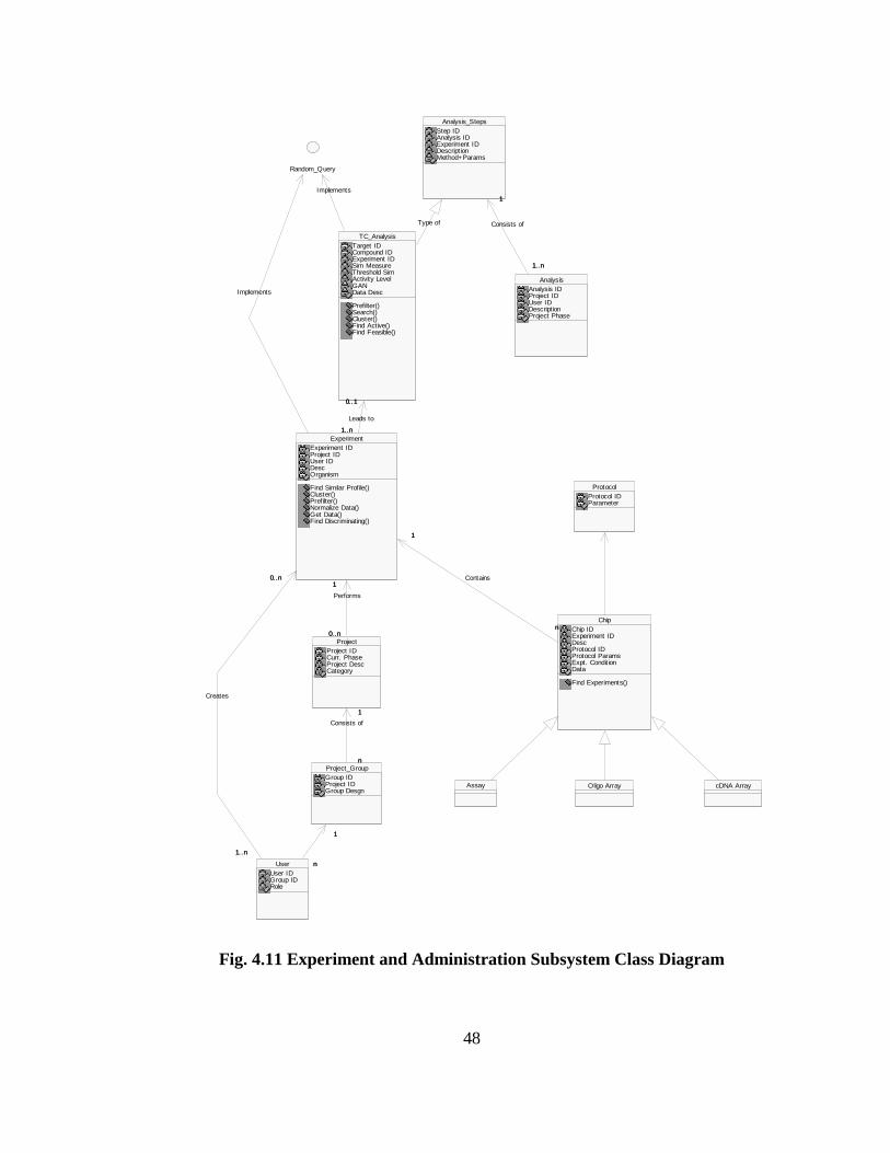
Finally, Fig. 4.11 shows the Administration and Experiment subsystems. The former
merely shows the relation between large projects with many project groups and users.
Details regarding user restrictions and other maintenance criteria are not discussed further
here. The Experiment subsystem links the User class with experiments conducted by an
individual. Each Experiment class object corresponds to many individual chips
(environmental conditions) and each chip is defined by a protocol and parameter set.
46
Fig. 4.9 Public Data Subsystem Class Diagram
Disease_Phenotype
Disease_IDNameCategorySummaryDiagnosisMolecular GeneticsResourcesReferencesClinical Description
Proteome_Info
Protein_IDGANProtein NameFunctional CategPost Trans ModificationsMolecular EnvtCellular RoleSubcel lular Function
EC_GAN
EC NumberGAN
MYGD_Class
ORFGene NameORF Description
Pathway
Pathway IDPathway NameSpeciesDiagram : BLOBCategory
Pathway_Map
Pathway IDLocation IDLLXLLYURXURY
1
1
1
1
Represents
Locus_GAN
Locus IDGAN
Enzyme
EC NumberEnzyme Name
1..n
1..n
1..n
1..n
Contains
1
1
1
1
Identified by
MYGD_Function
Class ID
Functional_Class
Class IDDescription
MYGD_Protein
Protein Class ID
Protein_Class
Protein Class IDDescription
47
Fig. 4.10 Target, Compound, and Analysis Subsystem Class Diagram
Target_Structure
Structure IDGeometry : Object
Find Similar Structure()
Compound_Structure
Structure IDGeometry : Object
Find Similar Compound()
ReceptorProtein
Target
Target IDNamePathwaysStructure IDDiseasesChemical Prop. : ObjectPhysical Prop. : ObjectReferences
Get Physical Property()Get Chemical Property()Predict Target Structure()
1
1
1
1
Corresponds to
Compound
Compound IDNameStructure IDCategoryChemical Prop. : ObjectFormulaPhysical Prop. : ObjectReferences
Find Similar Target()Predict ADME Property()Predict Chemical Property()Predict Physical Property()Get Physical Property()Get Chemical Property()
Corresponds to
TC_Analysis
Target IDCompound IDExperiment IDSim MeasureThreshold SimActivity LevelGANData Desc
Prefil ter()Search()Cluster()Find Active()Find Feasible()
1
n
1
n
1
n
Analysis
Analysis IDProject IDUser IDDescriptionProject Phase
Analysis_Steps
Step IDAnalysis IDExperiment IDDescriptionMethod+Params
Consists of
Type of
Implements
Random_Query
48
Fig. 4.11 Experiment and Administration Subsystem Class Diagram
Assay Oligo Array cDNA Array
ProtocolProtocol IDParameter
Project_GroupGroup IDProject IDGroup Desgn
ChipChip IDExperiment IDDescProtocol IDProtocol ParamsExpt. ConditionData
Find Experiments()
UserUser IDGroup IDRole
ProjectProject IDCurr. PhaseProject DescCategory
TC_AnalysisTarget IDCompound IDExperiment IDSim MeasureThreshold SimActivity LevelGANData Desc
Prefilter()Search()Cluster()Find Active()Find Feasible()
Random_Query
ExperimentExperiment IDProject IDUser IDDescOrganism
Find Similar Profile()Cluster()Prefilter()Normalize Data()Get Data()Find Discriminating()
Analysis_StepsStep IDAnalysis IDExperiment IDDescriptionMethod+Params
AnalysisAnalysis IDProject IDUser IDDescriptionProject Phase
1
n
1
n
1
n
1
n
Consists of
Implements
1
n
1
n
Contains0..n
1..n
0..n
1..n
Creates
1
0..n
1
0..n
Performs
0..1
1..n
0..1
1..n
Leads to
Implements
Type of
1
1..n
1
1..n
Consists of
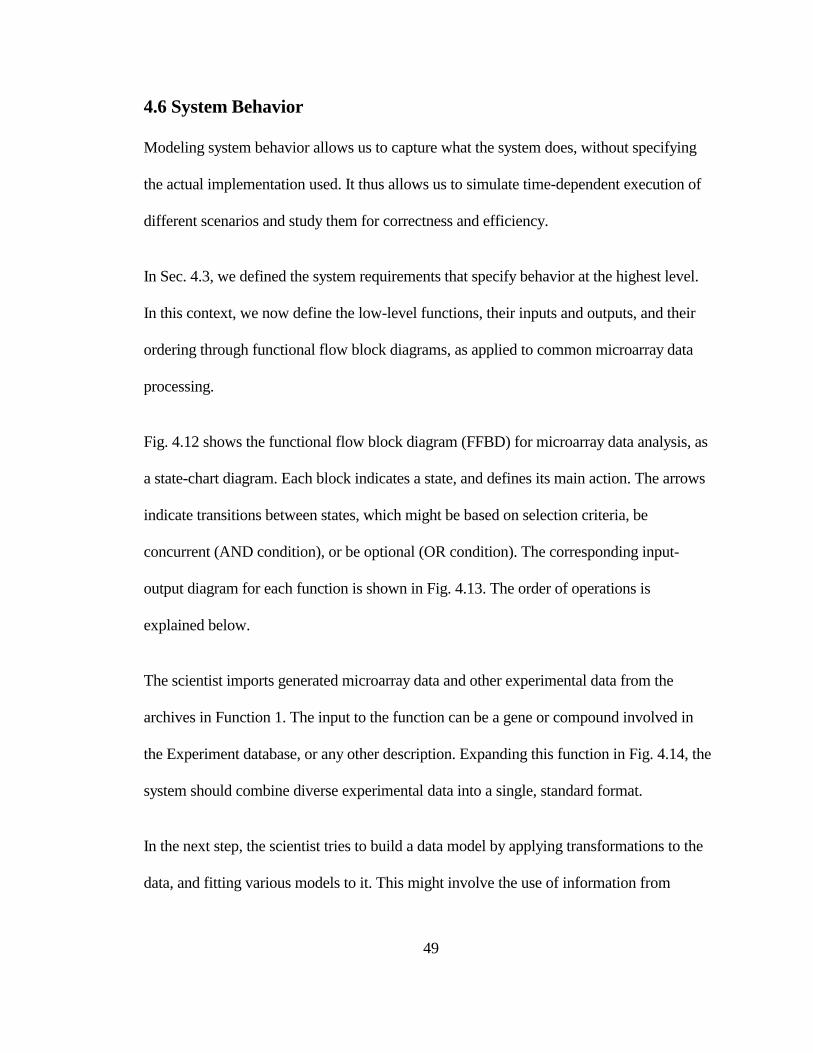
49
4.6 System Behavior
Modeling system behavior allows us to capture what the system does, without specifying
the actual implementation used. It thus allows us to simulate time-dependent execution of
different scenarios and study them for correctness and efficiency.
In Sec. 4.3, we defined the system requirements that specify behavior at the highest level.
In this context, we now define the low-level functions, their inputs and outputs, and their
ordering through functional flow block diagrams, as applied to common microarray data
processing.
Fig. 4.12 shows the functional flow block diagram (FFBD) for microarray data analysis, as
a state-chart diagram. Each block indicates a state, and defines its main action. The arrows
indicate transitions between states, which might be based on selection criteria, be
concurrent (AND condition), or be optional (OR condition). The corresponding input-
output diagram for each function is shown in Fig. 4.13. The order of operations is
explained below.
The scientist imports generated microarray data and other experimental data from the
archives in Function 1. The input to the function can be a gene or compound involved in
the Experiment database, or any other description. Expanding this function in Fig. 4.14, the
system should combine diverse experimental data into a single, standard format.
In the next step, the scientist tries to build a data model by applying transformations to the
data, and fitting various models to it. This might involve the use of information from

50
external sources like sequence and structure databases, and the use of visualization tools as
detailed in Fig. 4.15.
He/she then picks clustering methods and applies the data transform appropriate to the data
model (Functions 6,7). A variety of filtering steps can be applied at this point to the data, to
eliminate redundant or noisy features and reduce the dimension of the dataset (Function 8).
Fig. 4.16 expands this function including filtering based on fold-variation, significant
features, and function. The output of this step is a significant subset of features, which is
used in clustering or classification in the next steps (Functions 9, 11).
The scientist analyzes the clusters obtained by unsupervised clustering using contextual
information from queries to external information sources (Fig. 4.17), while he uses the
results of supervised classification directly for performance evaluation. For each type of
dataset, he/she tries different algorithms and varies their parameters. He/she then generates
a report of the findings and conclusions of the analysis, which can be made available to
other groups within the organization.

51
Fig. 4.12 State-chart Diagram for Behavior
(1) do: Import experimental data
(2) do: Search and link public-domain information
(5) do: Build the data model
(6) do: Choose an appropriate clustering method for the model
(8) do: Filter data by specifying the statistical criteria to pick a reduced set of features
(12) do: Measure performance
(13) do: Generate and store analysis reports
(4) do: Generate visualizations
(3) do: Apply a data transform
(7) do: Apply the data transform
(9) do: Apply the unsupervised clustering algorithm (11) do: Perform supervised
classification to discriminate classes
(10) do: Validate and review the clusters
OR
AND
AND
Done
Repeat with a different algorithm
Repeat with new parameters
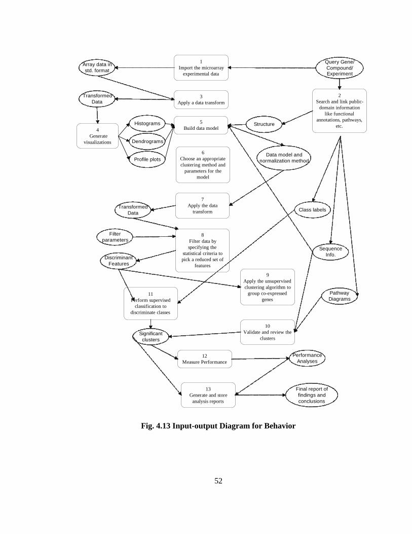
52
Fig. 4.13 Input-output Diagram for Behavior
1Import the microarray
experimental data
2Search and link public-
domain informationlike functional
annotations, pathways,etc.
5Build data model
6Choose an appropriateclustering method and
parameters for themodel
7Apply the data
transform
8Filter data byspecifying the
statistical criteria topick a reduced set of
features
9Apply the unsupervisedclustering algorithm to
group co-expressedgenes
12Measure Performance
13Generate and store
analysis reports
4 Generate
visualizations
3Apply a data transform
10Validate and review the
clusters
11Perform supervised
classification todiscriminate classes
Query Gene/Compound/Experiment
Array data instd. format
SequenceInfo.
PathwayDiagrams
Class labels
Histograms
Dendrograms
TransformedData
Profile plots
DiscriminantFeatures
Significantclusters
TransformedData
PerformanceAnalyses
Final report offindings andconclusions
Data model andnormalization method
Filterparameters
Structure
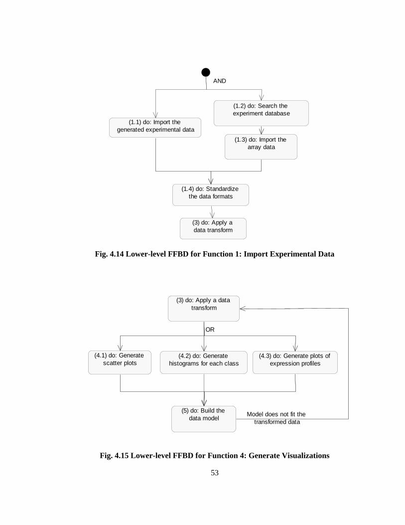
53
Fig. 4.14 Lower-level FFBD for Function 1: Import Experimental Data
Fig. 4.15 Lower-level FFBD for Function 4: Generate Visualizations
(1.1) do: Import the generated experimental data
(1.2) do: Search the experiment database
(1.3) do: Import the array data
(1.4) do: Standardize the data formats
AND
(3) do: Apply a data transform
(4.1) do: Generate scatter plots
(4.2) do: Generate histograms for each class
(4.3) do: Generate plots of expression profiles
(3) do: Apply a data transform
(5) do: Build the data model
OR
Model does not fit the transformed data
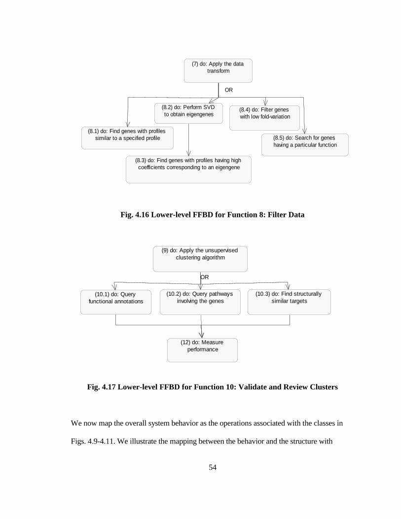
54
Fig. 4.16 Lower-level FFBD for Function 8: Filter Data
Fig. 4.17 Lower-level FFBD for Function 10: Validate and Review Clusters
We now map the overall system behavior as the operations associated with the classes in
Figs. 4.9-4.11. We illustrate the mapping between the behavior and the structure with
(7) do: Apply the data transform
(8.1) do: Find genes with profiles similar to a specified profile
(8.2) do: Perform SVD to obtain eigengenes
(8.3) do: Find genes with profiles having high coefficients corresponding to an eigengene
(8.4) do: Filter genes with low fold-variation
(8.5) do: Search for genes having a particular function
OR
(10.1) do: Query functional annotations
(10.2) do: Query pathways involving the genes
(10.3) do: Find structurally similar targets
(9) do: Apply the unsupervised clustering algorithm
(12) do: Measure performance
OR
55
examples from the class diagrams. By indexing over target structure, it is possible to obtain
targets with high structural similarity to a known one. This is defined in the
FindSimilarStructure() operation of the Target_Structure class. Other related functions are
FindSimilarCompound() in the Compound_Structure class, and FindSimilarProfile() in the
Experiment class.
The operations on the Compound class like PredictADMEProperties() are derived from the
use case scenarios for the computational biologist/chemist. Such queries might also involve
other subsystems and require indexing across heterogeneous databases.
It is also important to note that the class diagrams above show only persistent object
structure, and their constraints and relationships. By associating persistent object behavior
with the database, the processing of array data can be handled by the DBMS itself. The
advantage of this technique is that processing can be carried out using the DBMS
optimizations in parallel with the application.
ORDBMS products like Oracle 8 emulate database server behavior by allowing the
operations to be coded in a database programming language like PL/SQL. The
implementation can also be performed in modules containing the class methods, such as
Oracle NCS Cartridges and Informix Data Blades. The features of the object-relational
model and database extensions are discussed in Sec. 4.8. Here, we list some of the common
data mining queries and the corresponding system responses derived from the UML
models:
56
(i) What are the characteristics of a disease? (pathways, active compounds, known
targets, disease phenotype, references)
(ii) What are the properties of known targets? (target type, structures, function,
chemical and geometric properties)
(iii) Which experiments in MicroarrayDB involve the known targets and
corresponding active compounds? (ExperimentID, data format, expression data)
(iv) Which genes have shown activity similar to known targets?
(v) Which genes are good discriminating instances across all experiments in a
dataset?
(vi) Which genes are likely to be drug targets from a set of experiments, given their
sequence and structure?
(vii) Which compounds are likely to show good activity, specificity and
pharmacological properties (for ADME tests) on these targets? (QSPR)
(viii) What compounds in the libraries are likely to give a comparable performance to
an existing product?
(ix) How will the activity of a compound be on a particular target given their
structure? (QSAR)
(x) Which drug research categories have high lead times?
4.7 System Architecture Summary
In this section, a variety of system architectures are studied, to determine how they meet
the high-level requirements outlined in Sec. 4.3.
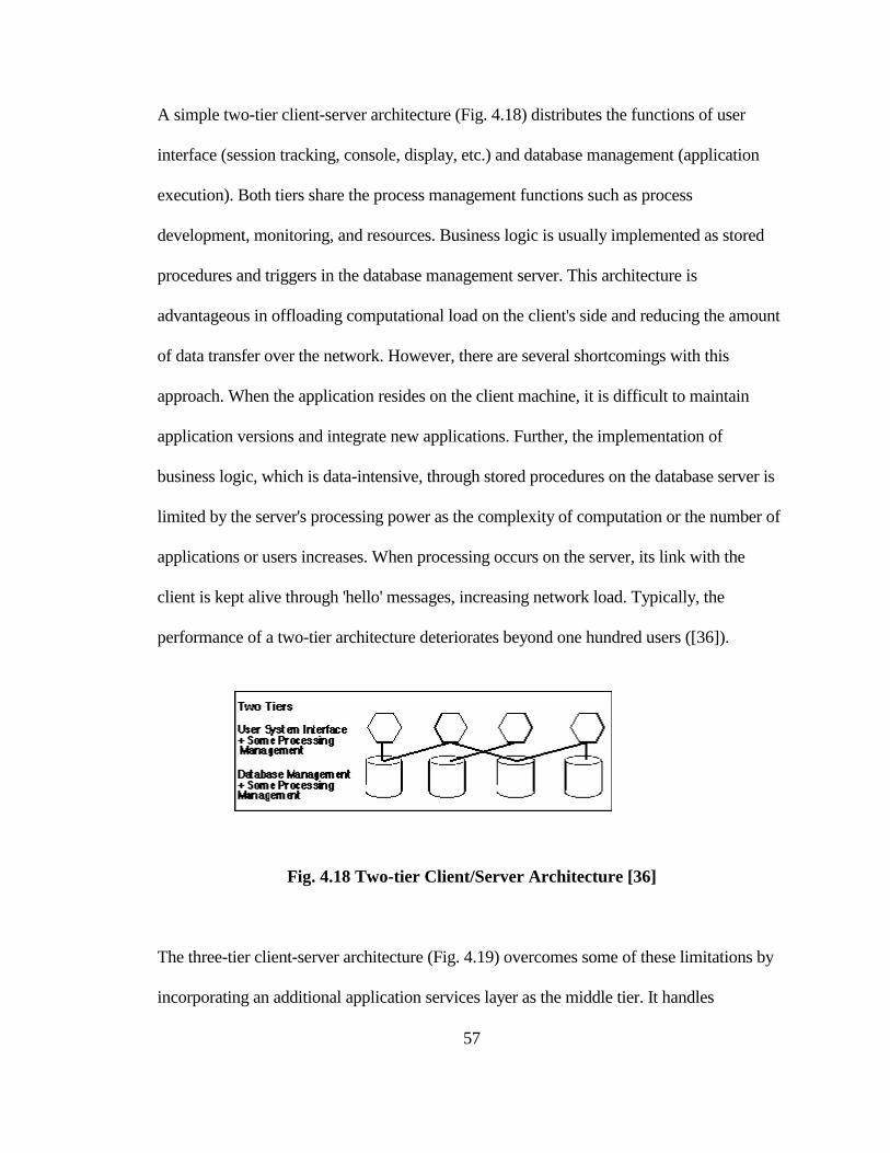
57
A simple two-tier client-server architecture (Fig. 4.18) distributes the functions of user
interface (session tracking, console, display, etc.) and database management (application
execution). Both tiers share the process management functions such as process
development, monitoring, and resources. Business logic is usually implemented as stored
procedures and triggers in the database management server. This architecture is
advantageous in offloading computational load on the client's side and reducing the amount
of data transfer over the network. However, there are several shortcomings with this
approach. When the application resides on the client machine, it is difficult to maintain
application versions and integrate new applications. Further, the implementation of
business logic, which is data-intensive, through stored procedures on the database server is
limited by the server's processing power as the complexity of computation or the number of
applications or users increases. When processing occurs on the server, its link with the
client is kept alive through 'hello' messages, increasing network load. Typically, the
performance of a two-tier architecture deteriorates beyond one hundred users ([36]).
Fig. 4.18 Two-tier Client/Server Architecture [36]
The three-tier client-server architecture (Fig. 4.19) overcomes some of these limitations by
incorporating an additional application services layer as the middle tier. It handles
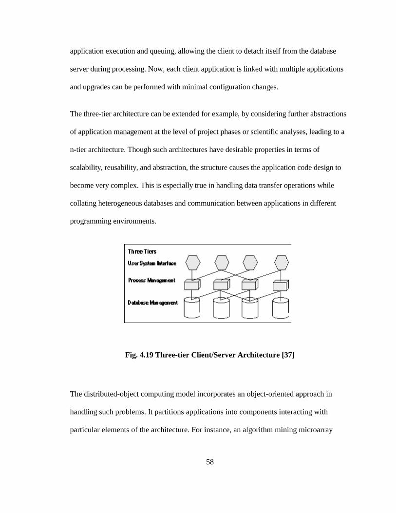
58
application execution and queuing, allowing the client to detach itself from the database
server during processing. Now, each client application is linked with multiple applications
and upgrades can be performed with minimal configuration changes.
The three-tier architecture can be extended for example, by considering further abstractions
of application management at the level of project phases or scientific analyses, leading to a
n-tier architecture. Though such architectures have desirable properties in terms of
scalability, reusability, and abstraction, the structure causes the application code design to
become very complex. This is especially true in handling data transfer operations while
collating heterogeneous databases and communication between applications in different
programming environments.
Fig. 4.19 Three-tier Client/Server Architecture [37]
The distributed-object computing model incorporates an object-oriented approach in
handling such problems. It partitions applications into components interacting with
particular elements of the architecture. For instance, an algorithm mining microarray
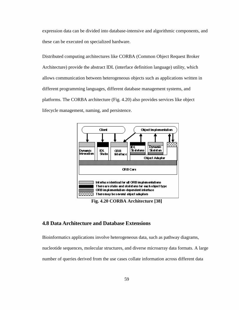
59
expression data can be divided into database-intensive and algorithmic components, and
these can be executed on specialized hardware.
Distributed computing architectures like CORBA (Common Object Request Broker
Architecture) provide the abstract IDL (interface definition language) utility, which
allows communication between heterogeneous objects such as applications written in
different programming languages, different database management systems, and
platforms. The CORBA architecture (Fig. 4.20) also provides services like object
lifecycle management, naming, and persistence.
Fig. 4.20 CORBA Architecture [38]
4.8 Data Architecture and Database Extensions
Bioinformatics applications involve heterogeneous data, such as pathway diagrams,
nucleotide sequences, molecular structures, and diverse microarray data formats. A large
number of queries derived from the use cases collate information across different data
60
types and finding patterns in uncommon data types like molecular structures, gene
expression, and so on.
The traditional relational data model is restrictive in modeling the structure of data and
such queries based on particular properties would need to be implemented as part of the
application behavior, thereby increasing complexity and execution time.
The object-relational data model provides several extensions to the relational and object-
oriented models:
• The ability to implement restrictions on data types as subtypes.
• Encapsulated data types, which can be extending from the base types, and can be
implemented by separate indexing and access methods.
• Complex objects and collections like nested tables, typed columns, references, and
function indices.
• More complex rule mechanisms compared to relational triggers.
The following examples show how object-relational database extensions can be designed
to handle bioinformatics queries:
• Operator and function notation in place of indices. E.g. NearestNeighbor()
• User-Defined Aggregates: E.g. Centroid (similarity)
• User-defined Comparison Operators: E.g. MoreSpecificThan()

61
CHAPTER 5: LEARNING ALGORITHMS
5.1 Introduction
In this chapter, we discuss a few algorithms that implement by the system behavior
described in the previous chapter. We begin with a description and properties of a new
similarity measure for gene expression data based on raw, un-normalized values, called the
Symmetric Kullback-Liebler similarity measure. In the later sections, we describe the
analysis methods.
5.2 Similarity Measures
The database behavior described in Chapter 4 required several algorithms involving search,
indexing, and clustering procedures. With a variety of microarray manufacturing
techniques, this requires the development of appropriate measures of similarity of gene
expression.
5.2.1 Microarray Expression Data
In particular, we look at two types of microarrays - cDNA and oligonucleotide arrays. An
expression value from a cDNA array represent the lognormal ratio of the amount of RNA
present in an experiment sample to that measured in a control sample. Oligonucleotide
array expression values indicate the average difference between (approximately 10)
replicate probe pairs containing the perfect match (PM) and mismatch (MM) values [7].
Because of manufacturing technique and standardization procedures, oligonucleotide arrays
have a very high reproducibility compared to cDNA arrays as explained in Sec. 3.1.1.
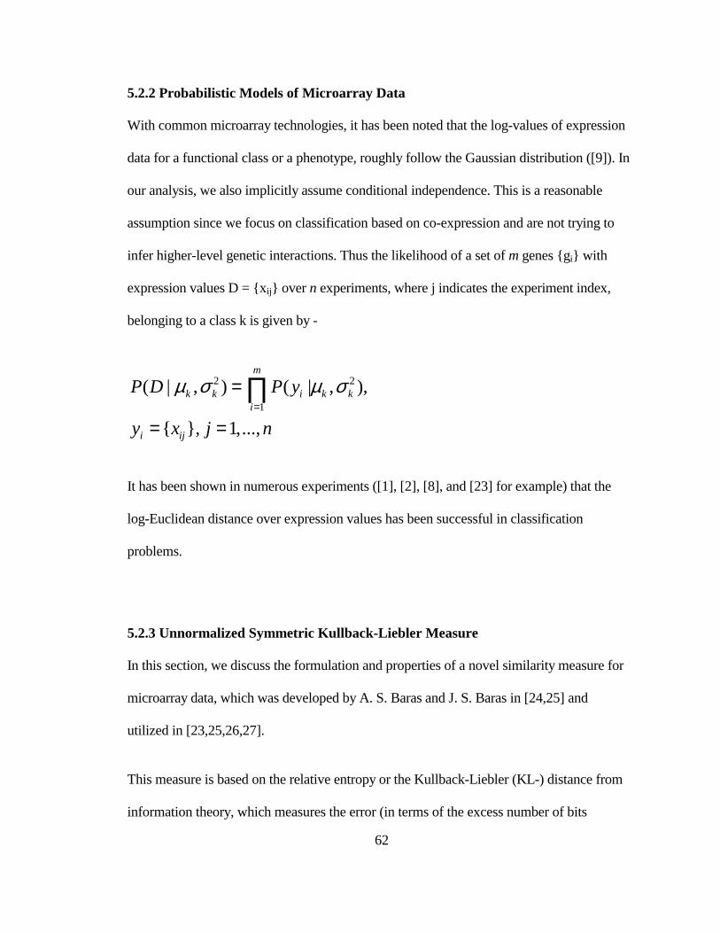
62
5.2.2 Probabilistic Models of Microarray Data
With common microarray technologies, it has been noted that the log-values of expression
data for a functional class or a phenotype, roughly follow the Gaussian distribution ([9]). In
our analysis, we also implicitly assume conditional independence. This is a reasonable
assumption since we focus on classification based on co-expression and are not trying to
infer higher-level genetic interactions. Thus the likelihood of a set of m genes {gi} with
expression values D = {xij} over n experiments, where j indicates the experiment index,
belonging to a class k is given by -
2 2
1
( | , ) ( | , ),
{ }, 1,...,
m
k k i k ki
i ij
P D P y
y x j n
µ σ µ σ=
=
= =
∏
It has been shown in numerous experiments ([1], [2], [8], and [23] for example) that the
log-Euclidean distance over expression values has been successful in classification
problems.
5.2.3 Unnormalized Symmetric Kullback-Liebler Measure
In this section, we discuss the formulation and properties of a novel similarity measure for
microarray data, which was developed by A. S. Baras and J. S. Baras in [24,25] and
utilized in [23,25,26,27].
This measure is based on the relative entropy or the Kullback-Liebler (KL-) distance from
information theory, which measures the error (in terms of the excess number of bits

63
needed) to represent a random variable with a distribution q, given that its true distribution
is p. For a random variable x, the KL-distance is given by
2 2
( ) ( )( || ) ( ) log log
( ) ( )px X
p x p xD p q p x E
q x q x∈
= =∑
The KL-distance is also known as relative entropy([30]). The relative entropy is
asymmetric and measures the deviation between the two distributions.
The unnormalized symmetric Kullback-Liebler measure quantifies the dissimilarity
between two expression indexes (over genes or experiments), so that it is symmetric and
there is no need for normalization of the expression data; its novelty is the latter property. It
is based on the un-normalized expression indexes like the average difference values in
oligonucleotide arrays and the fluorescence ratio of Cy5 to Cy3 in cDNA arrays. We follow
[24,25] in describing it here.
Definition ([24,25]): The unnormalized symmetric Kullback-Liebler measure between two
expression vectors x and y of length N is defined as
1
log( ) log( )1( || )
2 log( ) log( )
, 0, 1,...,
Ni i
i ii i i
i i
x yD x y x y
y x
x y i N
=
= +
> =
∑
Properties ([24,25]):
1. ( || ) 0D x y ≥ , if , 0, 1,...,i ix y i N> =

64
( || ) 0D x y = , iff i ix y i= ∀
2. ( || )D x y is convex in the pair (x, y).
1 2 1 2 1 1 1 1( (1 ) || (1 ) ) ( || ) (1 ) ( || )D x x y y D x y D x yλ λ λ λ λ λ+ − + − ≤ + − , where 0 1λ≤ ≤
3. There exists a unique centroid c of a set kS = {x }, k=1,...K of vectors of length N
based on the unnormalized symmetric Kullback-Liebler measure given by the
solution of the following equation ([24,25]).
�
ln 1, 1,...,i i
ii
c xi N
cx= − = , where
1 ki i
k
x xK
= ∑ is the arithmetic mean, and �1
exp ln( )ki i
k
x xK
=
∑ is the geometric
mean. Further, the centroid is bounded by the two means:
� , 1,...,i i ix c x i N≤ ≤ =
The unnormalized symmetric Kullback-Liebler measure describes quantitatively the
dissimilarities between two expression vectors x and y, assuming either is the true
distribution. It combines the value difference and fold variation (log-values) between the
two vectors, and can lead to a more accurate prediction across classes where genes have
widely varying levels of expression. With reference to the planar separating surfaces
formed by the log-Euclidean distance during classification, we note that the unnormalized
symmetric Kullback-Liebler measure leads to non-linear hyper-surfaces.
65
5.3 Learning Algorithms
In this section, we look at specific algorithms for different types of gene expression
analyses. The chief properties of such algorithms should include:
• Minimum inductive bias.
• Ability to handle noisy and irrelevant attributes, and outliers.
• Ability to handle different similarity measures.
• Good initial hypothesis.
• Ability to generalize well with limited training data.
5.3.1 LBG/LVQ Algorithm
The Linde-Buzo-Gray algorithm (LBG) or the Generalized Lloyd algorithm [19] is a signal
approximation algorithm, which generates a codebook of centroid vectors. We use LBG for
unsupervised clustering in a tree-structured manner ([15]). The algorithm starts with a
representative pattern of gene expression for the entire dataset and partitions the pattern
space by applying small perturbations at each successive node. At the same time, it
iteratively optimizes the codebook at each level until the centroids at the level are
stationary. The stopping rule for LBG is based on the percentage decrease in the overall
distortion. The algorithm steps are listed below.
1. Given the input matrix MxNX , initial learning rate ε , fix the number of codevectors
K = 1 and the tree depth L=1.

66
1 ( )c centroid X=
21
1
1 11 11 11
1|| || ,Euclidean distance
11[( )(log( ) log( ))],( , )
unnormalized symmetric Kullback-Liebler
measure
N
nn
N MN
nm m nm mnn mn
x cNM
x c x cErr dist x cNMNM
=
= ==
− − −= =
∑
∑∑∑
2. Node splitting: Set 2K K= , L=1, and for k=1,2,…K, initialize the codevectors at
the next level by
0
0
(1 )
(1 )k k
K k k
c c
c c
εε+
= −
= +
3. Set the iteration index i=0 and ( )
1i
LErr Err= .
(i) Find the closest centroid to each data vector xl and the associated class C(xl) as
( ) arg min( ( , ))i il l k
k
C x dist x c= .
(ii) Update the codevector for the K classes. For k=1,…,K,
1 ({ : , ( ) })i ikc centroid x x X C x k+ = ∈ = .
Set i = i + 1 and evaluate the new error iLErr .
(iii) If 1 1( ) /i i iL L LErr Err Err ε− −− > , go to step (i). Otherwise, for k=1,…,K, set i
k kc c= .
4. Repeat steps 2 and 3 until the desired number of levels is reached.
Learning vector quantization (LVQ) [18,28,29] is a neural network learning method, which
uses the nearest neighbor rule to train the codebook. Its inductive bias simply states that the
code vectors of a class are closer to its instances.
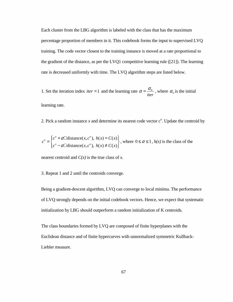
67
Each cluster from the LBG algorithm is labeled with the class that has the maximum
percentage proportion of members in it. This codebook forms the input to supervised LVQ
training. The code vector closest to the training instance is moved at a rate proportional to
the gradient of the distance, as per the LVQ1 competitive learning rule ([21]). The learning
rate is decreased uniformly with time. The LVQ algorithm steps are listed below.
1. Set the iteration index 1iter = and the learning rate 0
iter
αα = , where 0α is the initial
learning rate.
2. Pick a random instance x and determine its nearest code vector co. Update the centroid by
distance( , ), ( ) ( )
distance( , ), ( ) ( )
o on
o o
c x c h x C xc
c x c h x C x
αα
+ ∇ = = − ∇ ≠
, where 0 1α≤ ≤ , h(x) is the class of the
nearest centroid and C(x) is the true class of x.
3. Repeat 1 and 2 until the centroids converge.
Being a gradient-descent algorithm, LVQ can converge to local minima. The performance
of LVQ strongly depends on the initial codebook vectors. Hence, we expect that systematic
initialization by LBG should outperform a random initialization of K centroids.
The class boundaries formed by LVQ are composed of finite hyperplanes with the
Euclidean distance and of finite hypercurves with unnormalized symmetric Kullback-
Liebler measure.

68
5.3.2 Support Vector Machines
Support vector machines (SVM)[12] are classifiers based on statistical learning theory,
which map the input space to a high-dimensional space of non-linear features. This
mapping is implicitly made via a kernel function and all the computation is performed with
the input space vectors.
The SVM training algorithm generates hyperplanes in the feature space, whose margin is
optimized to obtain good generalization. Consider a data set composed of N expression
vectors <xi, yi>, where yi denotes the label for the data vector xi. Using the notation from
[11], the problem of finding the weight vector w can be formulated as minimizing the
function
21( ) || ||
2L w w= , subject to [ ]. ( ) 1, 1,..., .i iy w x b i Nφ + ≥ =
Here, the function ( )xφ maps the input vector to the feature vector. The dual formulation is
given by maximizing
1 1 1
1( ) ( , )
2
N N N
i i j i j i ji i j
Q y y K x xα α α α= = =
= −∑ ∑∑ subject to
1
0N
i ii
yα=
=∑ and 0 , 1,..., .i C i Nα≤ ≤ =
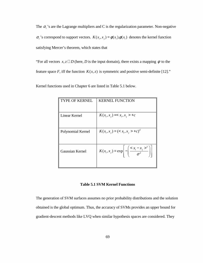
69
The iα ’s are the Lagrange multipliers and C is the regularization parameter. Non-negative
iα ’s correspond to support vectors. ( , ) ( ). ( )i j i iK x x x xφ φ= denotes the kernel function
satisfying Mercer’s theorem, which states that
“For all vectors ,x z D∈ (here, D is the input domain), there exists a mapping φ to the
feature space F, iff the function ( , )K x z is symmetric and positive semi-definite [12].”
Kernel functions used in Chapter 6 are listed in Table 5.1 below.
TYPE OF KERNEL KERNEL FUNCTION
Linear Kernel ( , ) ,i j i jK x x x x c=< > +
Polynomial Kernel ( , ) ( , )di j i jK x x x x c= < > +
Gaussian Kernel 2
2( , ) exp i j
i j
x xK x x
σ < − >
= −
Table 5.1 SVM Kernel Functions
The generation of SVM surfaces assumes no prior probability distributions and the solution
obtained is the global optimum. Thus, the accuracy of SVMs provides an upper bound for
gradient-descent methods like LVQ when similar hypothesis spaces are considered. They
70
also have good generalization properties because SVM training minimizes the empirical
risk for a chosen hypothesis space.
Choosing a particular kernel function imposes a restriction bias on the analysis. Another
limitation is illustrated by the fact that the unnormalized symmetric Kullback-Liebler
measure does not satisfy Mercer’s conditions and cannot be represented as a kernel
function.
5.3.2 IB3 Algorithm
The IB3 algorithm developed by Aha et al. ([13]) is an instance-based learning algorithm.
It classifies new instances in a lazy manner, using a set of representative stored instances
called the concept description. The nearest neighbor rule is used to associate the test data to
the class of the closest stored instance.
IB3 eliminates the high computational cost involved in the testing phase of instance-based
methods by storing instances with good predictive strengths. In the training phase, the
algorithm stores misclassified instances in the concept description and associates a
classification accuracy for all instances. The algorithm performs a statistical test to accept
or reject new instances based on the classification accuracy and the prevalence of the
instance’s true class, thus eliminating noisy data. The final concept description generated
after one epoch is thus likely to contain instances a little farther from the class boundary
than methods like IB2, which store all misclassified instances. The algorithm steps are
described below.
1. Initiate the concept description CD φ= .
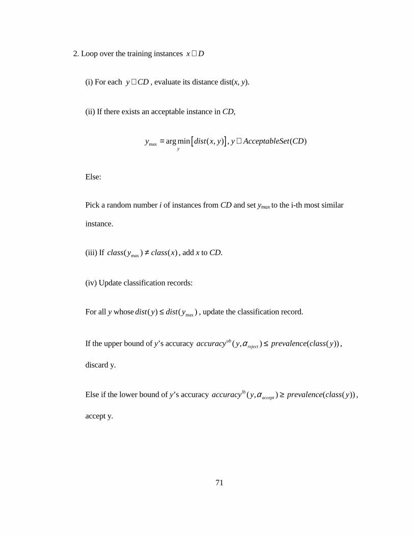
71
2. Loop over the training instances x D∈
(i) For each y CD∈ , evaluate its distance dist(x, y).
(ii) If there exists an acceptable instance in CD,
[ ]max arg min ( , ) , ( )y
y dist x y y AcceptableSet CD= ∈
Else:
Pick a random number i of instances from CD and set ymax to the i-th most similar
instance.
(iii) If max( ) ( )class y class x≠ , add x to CD.
(iv) Update classification records:
For all y whose max( ) ( )dist y dist y≤ , update the classification record.
If the upper bound of y’s accuracy ( , ) ( ( ))ubrejectaccuracy y prevalence class yα ≤ ,
discard y.
Else if the lower bound of y’s accuracy ( , ) ( ( ))lbacceptaccuracy y prevalence class yα ≥ ,
accept y.
72
In [13], Aha et al. have shown that the concept description set stores instances with high
classification accuracy, robustness, noise insensitivity, and high utilization (in terms of
classifying other instances during training).
IB3 has a restriction bias towards convex concepts. It shows poor performance with sparse
data sets, and is very sensitive to irrelevant attributes. However, it has minimal inductive
bias as it can approximate class boundaries with piecewise linear surfaces (with the
Euclidean distance). This feature makes it suitable, for example, to learn informative
instances in pre-filtering steps. Compared to IB3, decision trees have a stronger bias as
their separating surfaces are hyper-rectangles.
73
CHAPTER 6: RESULTS
6.1 Objectives
The aims of the experiments described in this chapter are as follows.
• Evaluate the performance of supervised classification of the LVQ algorithm with
LBG codebook initialization and SVMs.
• Compare the unnormalized symmetric Kullback-Liebler measure against Euclidean
distance in similarity-based algorithms with oligonucleotide arrays (the Find
Similar function).
• Evaluate the performance of the similarity measures in retrieving informative
instances (the Find Discriminating function).
• Conduct experiments on two applications of expression analysis - gene functional
classification and phenotype classification.
6.2 Description of Microarray Data
The three datasets used in testing the algorithms denote distinct applications in microarray
expression analysis, namely, phenotype classification and functional classification.
6.2.1 Lymphoma Dataset
The lymphoma cDNA array dataset comprises gene expression patterns of genes involved
in different classes of lymphoma and normal cell lines from Alizadeh et al [1].
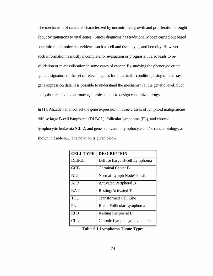
74
The mechanism of cancer is characterized by uncontrolled growth and proliferation brought
about by mutations to vital genes. Cancer diagnosis has traditionally been carried out based
on clinical and molecular evidence such as cell and tissue type, and heredity. However,
such information is mostly incomplete for evaluation or prognosis. It also leads to re-
validation or re-classification in some cases of cancer. By studying the phenotype or the
genetic signature of the set of relevant genes for a particular condition, using microarray
gene expression data, it is possible to understand the mechanism at the genetic level. Such
analysis is related to pharmacogenomic studies to design customized drugs.
In [1], Alizadeh et al collect the gene expression in three classes of lymphoid malignancies:
diffuse large B-cell lymphoma (DLBCL), follicular lymphoma (FL), and chronic
lymphocytic leukemia (CLL), and genes relevant to lymphocyte and/or cancer biology, as
shown in Table 6.1. The notation is given below.
CELL TYPE DESCRIPTION
DLBCL Diffuse Large B-cell Lymphoma
GCB Germinal Center B
NLT Normal Lymph Node/Tonsil
APB Activated Peripheral B
RAT Resting/Activated T
TCL Transformed Cell Line
FL B-cell Follicular Lymphoma
RPB Resting Peripheral B
CLL Chronic Lymphocytic Leukemia
Table 6.1 Lymphoma Tissue Types
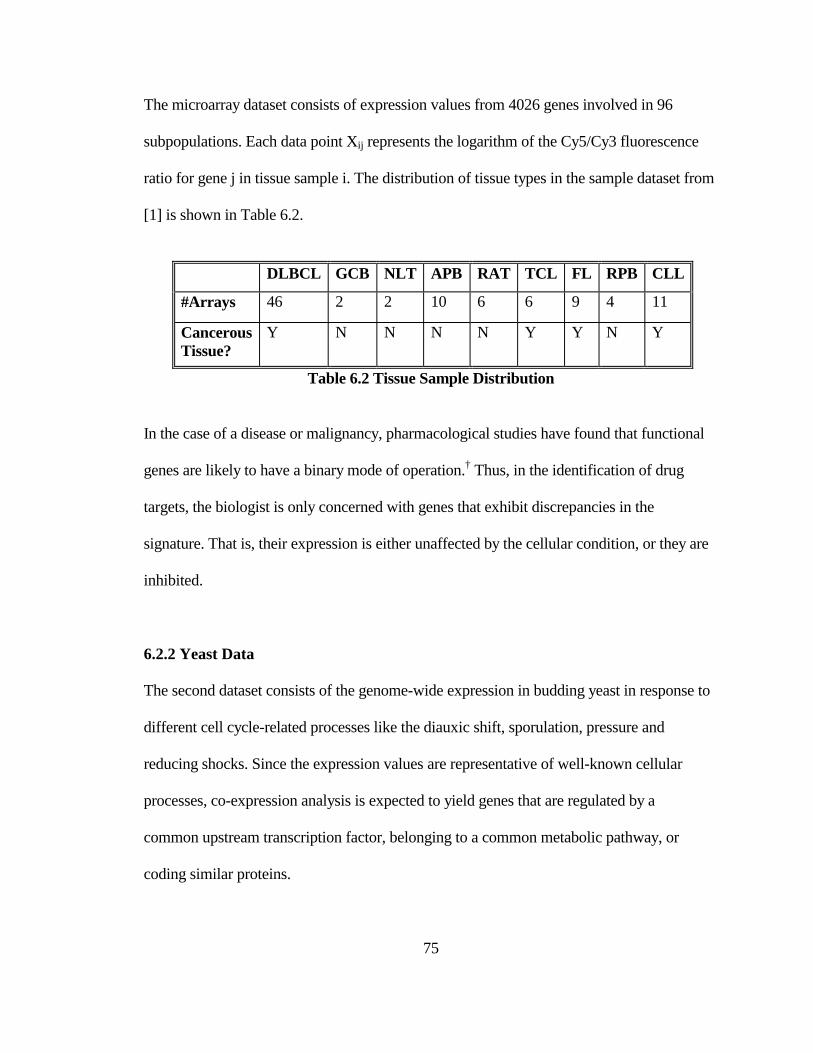
75
The microarray dataset consists of expression values from 4026 genes involved in 96
subpopulations. Each data point Xij represents the logarithm of the Cy5/Cy3 fluorescence
ratio for gene j in tissue sample i. The distribution of tissue types in the sample dataset from
[1] is shown in Table 6.2.
DLBCL GCB NLT APB RAT TCL FL RPB CLL
#Arrays 46 2 2 10 6 6 9 4 11
Cancerous Tissue?
Y N N N N Y Y N Y
Table 6.2 Tissue Sample Distribution
In the case of a disease or malignancy, pharmacological studies have found that functional
genes are likely to have a binary mode of operation.† Thus, in the identification of drug
targets, the biologist is only concerned with genes that exhibit discrepancies in the
signature. That is, their expression is either unaffected by the cellular condition, or they are
inhibited.
6.2.2 Yeast Data
The second dataset consists of the genome-wide expression in budding yeast in response to
different cell cycle-related processes like the diauxic shift, sporulation, pressure and
reducing shocks. Since the expression values are representative of well-known cellular
processes, co-expression analysis is expected to yield genes that are regulated by a
common upstream transcription factor, belonging to a common metabolic pathway, or
coding similar proteins.
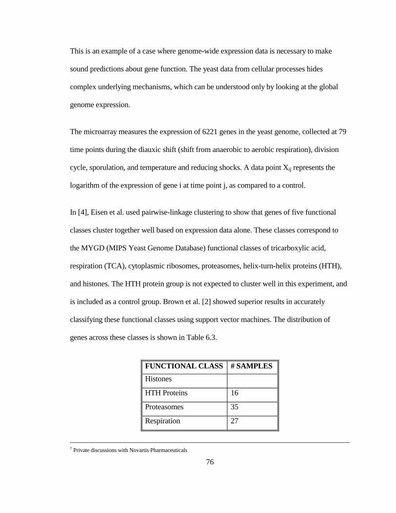
76
This is an example of a case where genome-wide expression data is necessary to make
sound predictions about gene function. The yeast data from cellular processes hides
complex underlying mechanisms, which can be understood only by looking at the global
genome expression.
The microarray measures the expression of 6221 genes in the yeast genome, collected at 79
time points during the diauxic shift (shift from anaerobic to aerobic respiration), division
cycle, sporulation, and temperature and reducing shocks. A data point Xij represents the
logarithm of the expression of gene i at time point j, as compared to a control.
In [4], Eisen et al. used pairwise-linkage clustering to show that genes of five functional
classes cluster together well based on expression data alone. These classes correspond to
the MYGD (MIPS Yeast Genome Database) functional classes of tricarboxylic acid,
respiration (TCA), cytoplasmic ribosomes, proteasomes, helix-turn-helix proteins (HTH),
and histones. The HTH protein group is not expected to cluster well in this experiment, and
is included as a control group. Brown et al. [2] showed superior results in accurately
classifying these functional classes using support vector machines. The distribution of
genes across these classes is shown in Table 6.3.
FUNCTIONAL CLASS # SAMPLES
Histones
HTH Proteins 16
Proteasomes 35
Respiration 27
† Private discussions with Novartis Pharmaceuticals
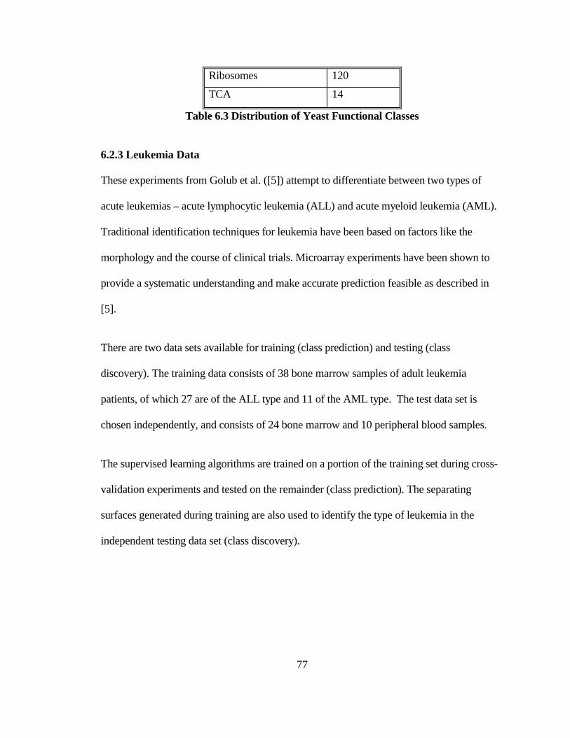
77
Ribosomes 120
TCA 14
Table 6.3 Distribution of Yeast Functional Classes
6.2.3 Leukemia Data
These experiments from Golub et al. ([5]) attempt to differentiate between two types of
acute leukemias – acute lymphocytic leukemia (ALL) and acute myeloid leukemia (AML).
Traditional identification techniques for leukemia have been based on factors like the
morphology and the course of clinical trials. Microarray experiments have been shown to
provide a systematic understanding and make accurate prediction feasible as described in
[5].
There are two data sets available for training (class prediction) and testing (class
discovery). The training data consists of 38 bone marrow samples of adult leukemia
patients, of which 27 are of the ALL type and 11 of the AML type. The test data set is
chosen independently, and consists of 24 bone marrow and 10 peripheral blood samples.
The supervised learning algorithms are trained on a portion of the training set during cross-
validation experiments and tested on the remainder (class prediction). The separating
surfaces generated during training are also used to identify the type of leukemia in the
independent testing data set (class discovery).
78
6.3 Methods
6.3.1 Supervised Classification
Supervised classification with LBG/LVQ, SVM, IB3, and C4.5 algorithms, is performed
using 3-fold cross-validation (except where indicated). Multiple runs with the data sets
have been used to determine parameters like the LVQ learning rate, number of epochs in
training, and the tree height in LBG.
The SVMTorch support vector machine software [31] used here is Ronan Collobert’s
implementation for large data sets and uses sequential minimal optimization (SMO). For
multi-class problems, SVMTorch trains each class with a one-over-all mechanism.
The IB3 algorithm implementation uses 90% and 68% confidence intervals for accepting
and rejecting instances respectively, when compared to the corresponding class frequency.
The C4.5 decision tree algorithm performs classification by repetitively choosing
attribute/value pairs, which minimize the overall entropy after partitioning the data space.
Quinlan’s information gain (or gain ratio to compensate diverse populations among classes)
can be used to select attributes at each step. The decision tree is then post-pruned based on
a user-specified threshold similarity, to avoid over-fitting.
6.3.2 Similarity-based Clustering
The log-Euclidean and the unnormalized symmetric Kullback-Liebler measures are
compared using a simple nearest-neighbor algorithm. We do not expect to see significant
differences in the performance with cDNA arrays, as against oligonucleotide arrays.

79
6.3.3 Comparison of Algorithms
In all methods described, we generate the confusion matrices and measure the overall
accuracy and the accuracy of individual classes.
The performance of two learning algorithms is compared by a t-test. The average error rate
of two learning algorithms 1L and 2L , trained and tested on the same data sets Sk and Tk is
given by
1 21
1( ( )) ( ( ))
k k
K
T k T kk
err L S err L SK
δ=
= − ∑ .
The N% confidence interval for δ to be an estimate of the true error difference is given by
, 1N Kt sδδ −± ,
where 2
1
1( )
( 1)
K
kk
sK Kδ δ δ
=
= −− ∑
and , 1N Kt − is the t-test value for two-sided confidence intervals [14].
6.4 Experiments
6.4.1 Lymphoma Data
Two types of classification are studied with the lymphoma data:
• Binary classification between cancerous and non-cancerous samples.
• Tissue type classification based on global gene expression.

80
In Cai et al.[3], differential analysis based on genes known to be involved in B-cell
lymphoma, has been shown to have no significant impact on the classifier’s ability to
recognize cancerous tissues. Hence, in both cases, we do not distinguish between the
selected genes based on prior knowledge. The C4.5 algorithm is expected to classify
cancerous tissues if the genetic signature of a subset of genes is a sufficient indicator.
Using the performance measure defined above, the results from the LVQ algorithm are
compared with those from other supervised learning techniques in [3], viz., SVM and C4.5
decision tree, using 10-fold cross-validation.
6.4.1.1 Binary Classification of Cancerous/Non-cancerous Tissues
For both cancer detection and tissue type identification (Section 6.4.1.2) experiments, the
initial codebook generated by the LBG algorithm consists of 16 code vectors and the LVQ
algorithm is trained for over 2 epochs.
Table 6.4 shows the typical performance of LVQ with the log-Euclidean distance for
cancer detection. These results on error average and variance are compared with results
from Cai et al. ([3]) using a linear-kernel SVM and a C4.5 decision tree. In Table 6.5, the
results from the LBG/LVQ algorithm are based on 10 cross-validation experiments, and
compare closely to the globally optimal SVM method. The LBG/LVQ algorithm gives a
much better and more stable performance compared to the C4.5 decision tree algorithm.
LVQ CLASSIFICATION
TRUE POSITIVE
TRUE NEGATIVE
FALSE POSITIVE
FALSE NEGATIVE
Cancerous Tissues 72 22 2 0 Non-cancerous Tissues 22 72 0 2
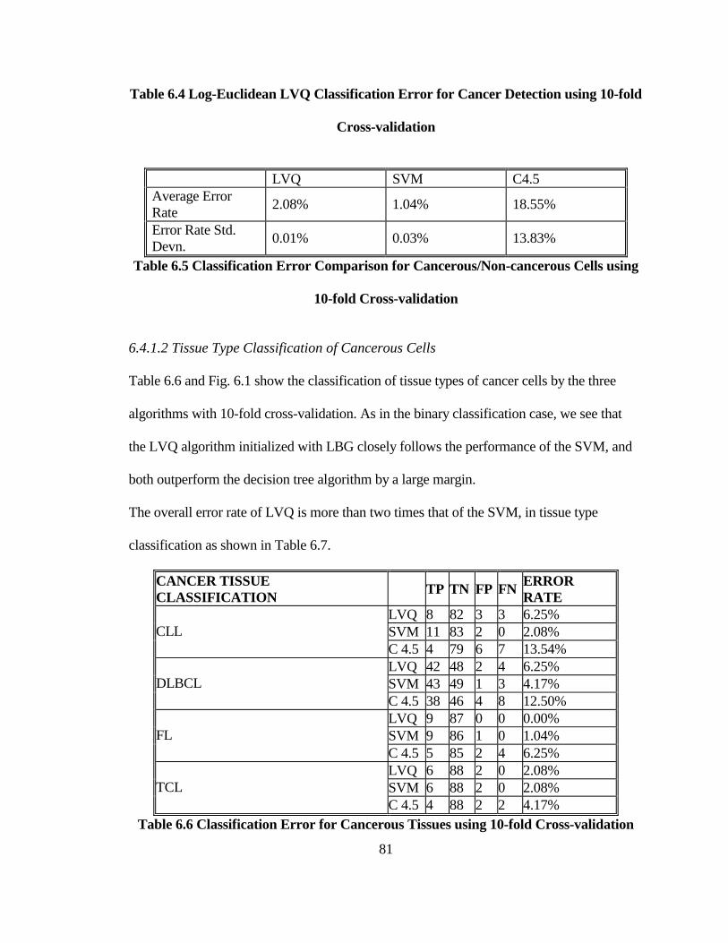
81
Table 6.4 Log-Euclidean LVQ Classification Error for Cancer Detection using 10-fold
Cross-validation
LVQ SVM C4.5 Average Error Rate
2.08% 1.04% 18.55%
Error Rate Std. Devn.
0.01% 0.03% 13.83%
Table 6.5 Classification Error Comparison for Cancerous/Non-cancerous Cells using
10-fold Cross-validation
6.4.1.2 Tissue Type Classification of Cancerous Cells
Table 6.6 and Fig. 6.1 show the classification of tissue types of cancer cells by the three
algorithms with 10-fold cross-validation. As in the binary classification case, we see that
the LVQ algorithm initialized with LBG closely follows the performance of the SVM, and
both outperform the decision tree algorithm by a large margin.
The overall error rate of LVQ is more than two times that of the SVM, in tissue type
classification as shown in Table 6.7.
CANCER TISSUE CLASSIFICATION
TP TN FP FN ERROR RATE
LVQ 8 82 3 3 6.25% SVM 11 83 2 0 2.08% CLL C 4.5 4 79 6 7 13.54% LVQ 42 48 2 4 6.25% SVM 43 49 1 3 4.17% DLBCL C 4.5 38 46 4 8 12.50% LVQ 9 87 0 0 0.00% SVM 9 86 1 0 1.04% FL C 4.5 5 85 2 4 6.25% LVQ 6 88 2 0 2.08% SVM 6 88 2 0 2.08% TCL C 4.5 4 88 2 2 4.17%
Table 6.6 Classification Error for Cancerous Tissues using 10-fold Cross-validation
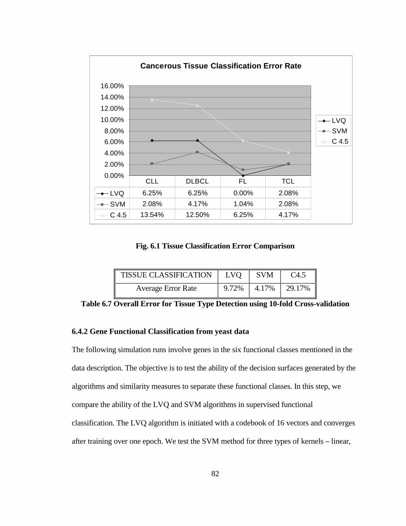
82
Fig. 6.1 Tissue Classification Error Comparison
TISSUE CLASSIFICATION LVQ SVM C4.5
Average Error Rate 9.72% 4.17% 29.17%
Table 6.7 Overall Error for Tissue Type Detection using 10-fold Cross-validation
6.4.2 Gene Functional Classification from yeast data
The following simulation runs involve genes in the six functional classes mentioned in the
data description. The objective is to test the ability of the decision surfaces generated by the
algorithms and similarity measures to separate these functional classes. In this step, we
compare the ability of the LVQ and SVM algorithms in supervised functional
classification. The LVQ algorithm is initiated with a codebook of 16 vectors and converges
after training over one epoch. We test the SVM method for three types of kernels – linear,
Cancerous Tissue Classification Error Rate
0.00%
2.00%
4.00%
6.00%
8.00%
10.00%
12.00%
14.00%
16.00%
LVQ
SVM
C 4.5
LVQ 6.25% 6.25% 0.00% 2.08%
SVM 2.08% 4.17% 1.04% 2.08%
C 4.5 13.54% 12.50% 6.25% 4.17%
CLL DLBCL FL TCL
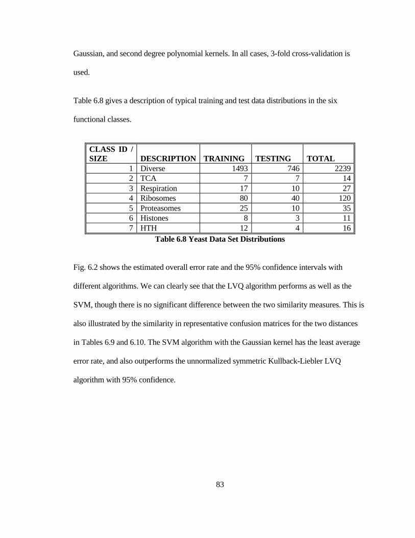
83
Gaussian, and second degree polynomial kernels. In all cases, 3-fold cross-validation is
used.
Table 6.8 gives a description of typical training and test data distributions in the six
functional classes.
CLASS ID / SIZE DESCRIPTION TRAINING TESTING TOTAL
1 Diverse 1493 746 2239 2 TCA 7 7 14 3 Respiration 17 10 27 4 Ribosomes 80 40 120 5 Proteasomes 25 10 35 6 Histones 8 3 11 7 HTH 12 4 16
Table 6.8 Yeast Data Set Distributions
Fig. 6.2 shows the estimated overall error rate and the 95% confidence intervals with
different algorithms. We can clearly see that the LVQ algorithm performs as well as the
SVM, though there is no significant difference between the two similarity measures. This is
also illustrated by the similarity in representative confusion matrices for the two distances
in Tables 6.9 and 6.10. The SVM algorithm with the Gaussian kernel has the least average
error rate, and also outperforms the unnormalized symmetric Kullback-Liebler LVQ
algorithm with 95% confidence.
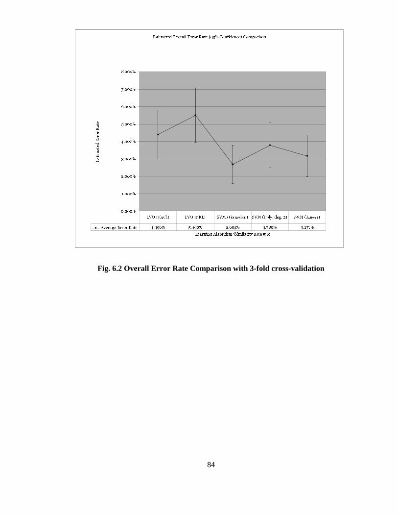
84
Fig. 6.2 Overall Error Rate Comparison with 3-fold cross-validation
Estimated Overall Error Rate (95% Confidence) Comparison
0.000%
1.000%
2.000%
3.000%
4.000%
5.000%
6.000%
7.000%
8.000%
Learning Algorithm/Similarity Measure
Estimated Error Rate
Average Error Rate 4.390% 5.490% 2.683% 3.780% 3.171%
LVQ (Eucl.) LVQ (SKL) SVM (Gaussian) SVM (Poly. deg. 2) SVM (Linear)
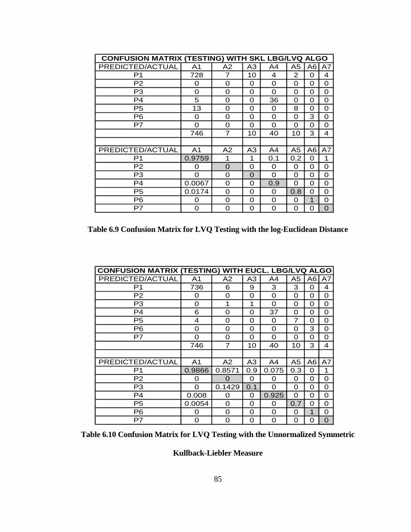
85
Table 6.9 Confusion Matrix for LVQ Testing with the log-Euclidean Distance
Table 6.10 Confusion Matrix for LVQ Testing with the Unnormalized Symmetric
Kullback-Liebler Measure
PREDICTED/ACTUAL A1 A2 A3 A4 A5 A6 A7P1 736 6 9 3 3 0 4P2 0 0 0 0 0 0 0P3 0 1 1 0 0 0 0P4 6 0 0 37 0 0 0P5 4 0 0 0 7 0 0P6 0 0 0 0 0 3 0P7 0 0 0 0 0 0 0
746 7 10 40 10 3 4
PREDICTED/ACTUAL A1 A2 A3 A4 A5 A6 A7P1 0.9866 0.8571 0.9 0.075 0.3 0 1P2 0 0 0 0 0 0 0P3 0 0.1429 0.1 0 0 0 0P4 0.008 0 0 0.925 0 0 0P5 0.0054 0 0 0 0.7 0 0P6 0 0 0 0 0 1 0P7 0 0 0 0 0 0 0
CONFUSION MATRIX (TESTING) WITH EUCL. LBG/LVQ ALGO
PREDICTED/ACTUAL A1 A2 A3 A4 A5 A6 A7P1 728 7 10 4 2 0 4P2 0 0 0 0 0 0 0P3 0 0 0 0 0 0 0P4 5 0 0 36 0 0 0P5 13 0 0 0 8 0 0P6 0 0 0 0 0 3 0P7 0 0 0 0 0 0 0
746 7 10 40 10 3 4
PREDICTED/ACTUAL A1 A2 A3 A4 A5 A6 A7P1 0.9759 1 1 0.1 0.2 0 1P2 0 0 0 0 0 0 0P3 0 0 0 0 0 0 0P4 0.0067 0 0 0.9 0 0 0P5 0.0174 0 0 0 0.8 0 0P6 0 0 0 0 0 1 0P7 0 0 0 0 0 0 0
CONFUSION MATRIX (TESTING) WITH SKL LBG/LVQ ALGO
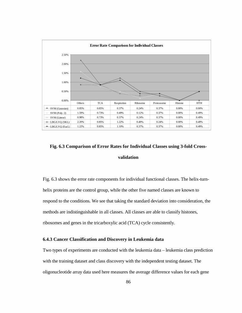
86
Fig. 6.3 Comparison of Error Rates for Individual Classes using 3-fold Cross-
validation
Fig. 6.3 shows the error rate components for individual functional classes. The helix-turn-
helix proteins are the control group, while the other five named classes are known to
respond to the conditions. We see that taking the standard deviation into consideration, the
methods are indistinguishable in all classes. All classes are able to classify histones,
ribosomes and genes in the tricarboxylic acid (TCA) cycle consistently.
6.4.3 Cancer Classification and Discovery in Leukemia data
Two types of experiments are conducted with the leukemia data – leukemia class prediction
with the training dataset and class discovery with the independent testing dataset. The
oligonucleotide array data used here measures the average difference values for each gene
Error Rate Comparison for Individual Classes
0.00%
0.50%
1.00%
1.50%
2.00%
2.50%
SVM (Gaussian) 0.85% 0.85% 0.37% 0.24% 0.37% 0.00% 0.00%
SVM (Poly. 2) 1.59% 0.73% 0.49% 0.12% 0.37% 0.00% 0.49%
SVM (Linear) 0.98% 0.73% 0.37% 0.24% 0.37% 0.00% 0.49%
LBG/LVQ (SKL) 2.20% 0.85% 1.22% 0.49% 0.24% 0.00% 0.49%
LBG/LVQ (Eucl.) 1.22% 0.85% 1.10% 0.37% 0.37% 0.00% 0.49%
Others TCA Respiration Ribosome Proteasome Histone HTH
87
in an experiment against a control. The pre-processing step involves setting negative
expression values to 20; we do not exclude genes marked absent in certain experiments.
We primarily study the Find Discriminating function (Use Case 1.2.1 in Sec. 4.4), which
tries to filter a small subset of genes, which are sufficient to predict a disease phenotype,
and which can be used to classify new phenotypes. We compare four different methods
using the following performance measures:
(i) Cross-validation error with the training set.
(ii) Overall error with the independent testing set.
(iii) Number of genes required obtaining certain prediction accuracy with the
independent testing set.
6.4.3.1 Prefiltering with the IB3 Algorithm
As in the method described in [5], we choose the ideal expression pattern as the one which
is uniformly high in the ALL experiments and low in the AML experiments, and vice-
versa. We then pick genes {g}, which have a close resemblance to this pattern c’, based on
the following similarity measure:
( , ')ALL AMLg g
ALL AMLg g
P g cµ µσ σ
−=
+
We picked an arbitrary absolute threshold value of 0.5 to prefilter leading to 1331 ‘active’
genes.
88
The class prediction tests now involve several steps:
• Cluster with the unsupervised LBG algorithm and label the genes based on the
initial codebook.
• Pick informative instances from the clusters using the IB3 algorithm.
• Filter acceptable stored instances with high predictive accuracy exceeding its class
frequency by a large margin.
• Use this set of ‘informative’ genes in clustering across experiments using the LVQ
and SVM algorithms.
Here, we note that we use the nearest neighbor rule to predict the class and do not take a
weighted vote from all the informative genes, as in [5].
The LBG algorithm divides the 1,331 genes into 4 clusters and the IB3 algorithm picks 59
and 66 instances of high-accuracy, with the log-Euclidean and the unnormalized symmetric
Kullback-Liebler measures respectively. The training data composed of expression
measurements of these genes across 38 types of leukemia, are used to train LVQ with 4
code vectors.
In a similar manner, the set of informative genes from the log-Euclidean distance based
filtering, is used to train SVMs.
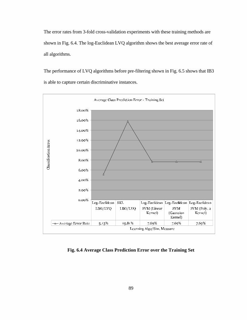
89
The error rates from 3-fold cross-validation experiments with these training methods are
shown in Fig. 6.4. The log-Euclidean LVQ algorithm shows the best average error rate of
all algorithms.
The performance of LVQ algorithms before pre-filtering shown in Fig. 6.5 shows that IB3
is able to capture certain discriminative instances.
Fig. 6.4 Average Class Prediction Error over the Training Set
Average Class Prediction Error - Training Set
0.00%
2.00%
4.00%
6.00%
8.00%
10.00%
12.00%
14.00%
16.00%
18.00%
Learning Algo/Sim. Measure
Classification Error
Average Error Rate 5.13% 15.81% 7.69% 7.69% 7.69%
Log-Euclidean SKL Log-Euclidean Log-Euclidean Log-Euclidean
LBG/LVQ LBG/LVQ SVM (Linear
Kernel)
SVM
(Gaussian
Kernel)
SVM (Poly. 2
Kernel)
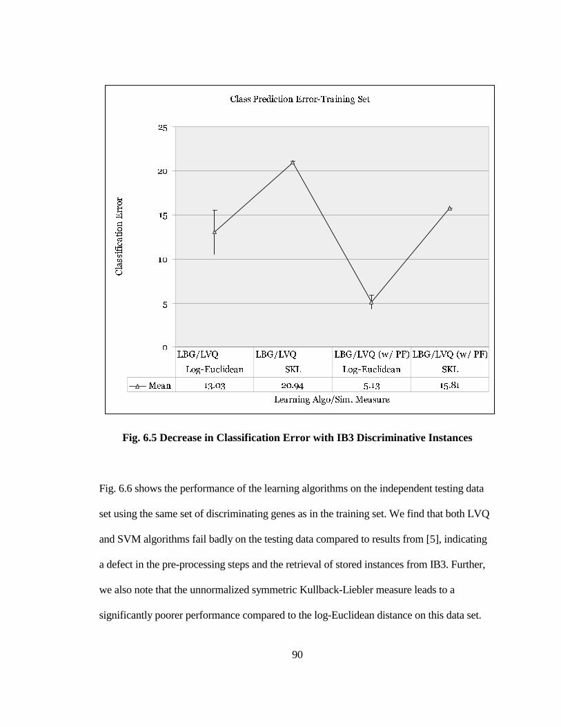
90
Fig. 6.5 Decrease in Classification Error with IB3 Discriminative Instances
Fig. 6.6 shows the performance of the learning algorithms on the independent testing data
set using the same set of discriminating genes as in the training set. We find that both LVQ
and SVM algorithms fail badly on the testing data compared to results from [5], indicating
a defect in the pre-processing steps and the retrieval of stored instances from IB3. Further,
we also note that the unnormalized symmetric Kullback-Liebler measure leads to a
significantly poorer performance compared to the log-Euclidean distance on this data set.
Class Prediction Error-Training Set
0
5
10
15
20
25
Learning Algo/Sim. Measure
Classification Error
Mean 13.03 20.94 5.13 15.81
LBG/LVQ LBG/LVQ LBG/LVQ (w/ PF) LBG/LVQ (w/ PF)
Log-Euclidean SKL Log-Euclidean SKL
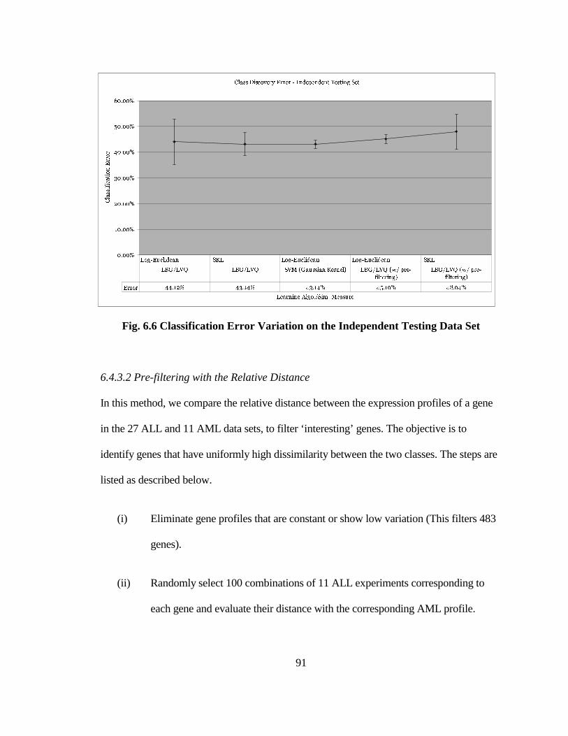
91
Fig. 6.6 Classification Error Variation on the Independent Testing Data Set
6.4.3.2 Pre-filtering with the Relative Distance
In this method, we compare the relative distance between the expression profiles of a gene
in the 27 ALL and 11 AML data sets, to filter ‘interesting’ genes. The objective is to
identify genes that have uniformly high dissimilarity between the two classes. The steps are
listed as described below.
(i) Eliminate gene profiles that are constant or show low variation (This filters 483
genes).
(ii) Randomly select 100 combinations of 11 ALL experiments corresponding to
each gene and evaluate their distance with the corresponding AML profile.
Class Discovery Error - Independent Testing Set
0.00%
10.00%
20.00%
30.00%
40.00%
50.00%
60.00%
Learning Algo./Sim. Measure
Classification Error
Error 44.12% 43.14% 43.14% 45.10% 48.04%
Log-Euclidean SKL Log-Euclidean Log-Euclidean SKL
LBG/LVQ LBG/LVQ SVM (Gaussian Kernel) LBG/LVQ (w/ pre-
filtering)
LBG/LVQ (w/ pre-
filtering)
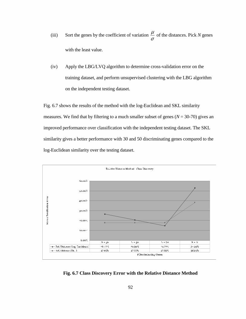
92
(iii) Sort the genes by the coefficient of variation µσ
of the distances. Pick N genes
with the least value.
(iv) Apply the LBG/LVQ algorithm to determine cross-validation error on the
training dataset, and perform unsupervised clustering with the LBG algorithm
on the independent testing dataset.
Fig. 6.7 shows the results of the method with the log-Euclidean and SKL similarity
measures. We find that by filtering to a much smaller subset of genes (N = 30-70) gives an
improved performance over classification with the independent testing dataset. The SKL
similarity gives a better performance with 30 and 50 discriminating genes compared to the
log-Euclidean similarity over the testing dataset.
Fig. 6.7 Class Discovery Error with the Relative Distance Method
Relative Distance Method - Class Discovery
0.00%
10.00%
20.00%
30.00%
40.00%
50.00%
60.00%
#Discriminating Genes
Mean Classification Error
Rel. Distance (Log-Euclidean) 26.47% 20.59% 14.71% 52.94%
Rel. Distance (SKL) 17.65% 17.65% 17.65% 38.24%
N = 30 N = 50 N = 70 N = M
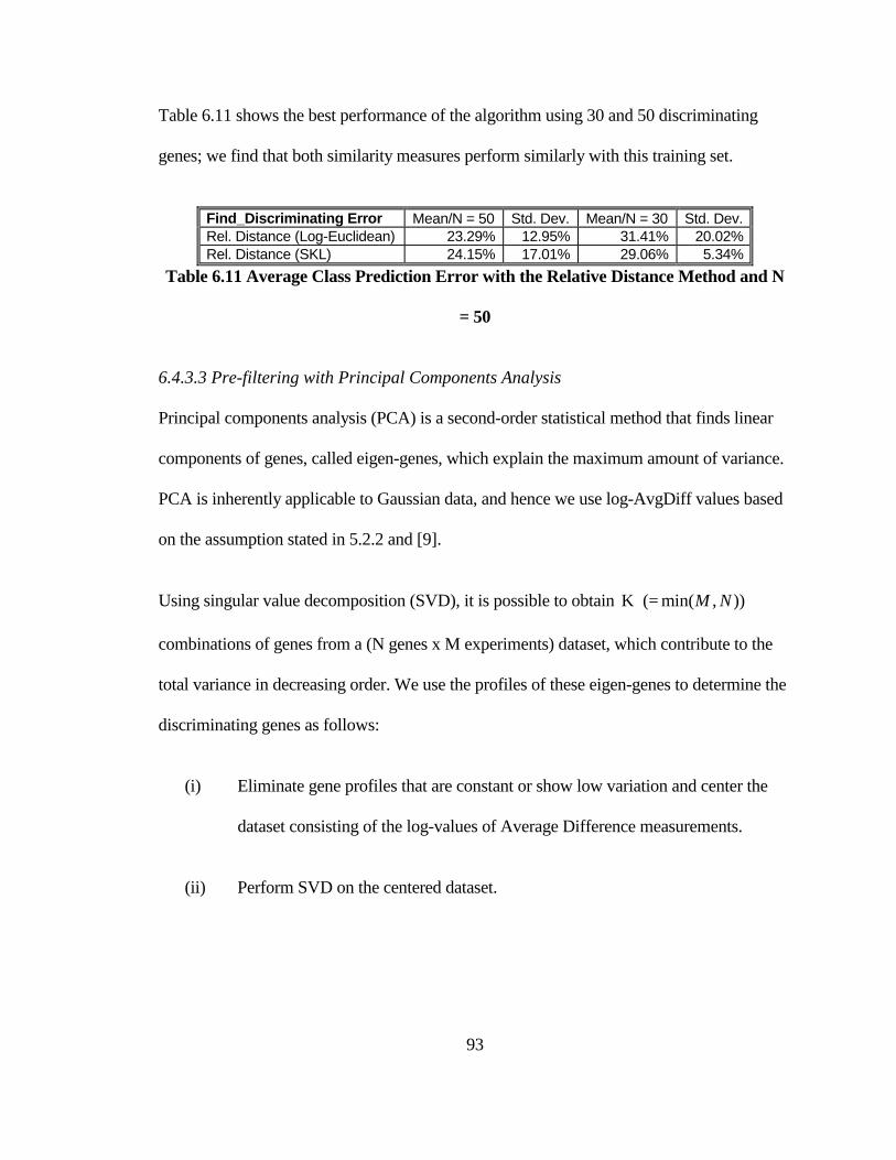
93
Table 6.11 shows the best performance of the algorithm using 30 and 50 discriminating
genes; we find that both similarity measures perform similarly with this training set.
Find_Discriminating Error Mean/N = 50 Std. Dev. Mean/N = 30 Std. Dev. Rel. Distance (Log-Euclidean) 23.29% 12.95% 31.41% 20.02% Rel. Distance (SKL) 24.15% 17.01% 29.06% 5.34%
Table 6.11 Average Class Prediction Error with the Relative Distance Method and N
= 50
6.4.3.3 Pre-filtering with Principal Components Analysis
Principal components analysis (PCA) is a second-order statistical method that finds linear
components of genes, called eigen-genes, which explain the maximum amount of variance.
PCA is inherently applicable to Gaussian data, and hence we use log-AvgDiff values based
on the assumption stated in 5.2.2 and [9].
Using singular value decomposition (SVD), it is possible to obtain K (= min( , ))M N
combinations of genes from a (N genes x M experiments) dataset, which contribute to the
total variance in decreasing order. We use the profiles of these eigen-genes to determine the
discriminating genes as follows:
(i) Eliminate gene profiles that are constant or show low variation and center the
dataset consisting of the log-values of Average Difference measurements.
(ii) Perform SVD on the centered dataset.

94
(iii) Pick the principal component PCi that explains a large proportion of the
variance and is closest to the ideal reference vector (uniformly high in one class
and low in the other).
(iv) Sort the genes that are closer to PCi than other principal components by their
correlation with PCi.
(v) Pick the top / 2N genes with high positive and negative correlations to obtain
the discriminating genes.
(v) Apply the LBG/LVQ algorithm to determine cross-validation error on the
training dataset, and perform unsupervised clustering with the LBG algorithm
on the independent testing dataset.
The results of PCA pre-filtering and classification with the two similarity measures are
shown in Fig. 6.8. We find that by filtering to a much smaller subset of genes (N = 30-70)
gives an improved performance in classification with the testing dataset. The SKL
similarity gives a marginally better performance with 30 and 50 discriminating genes
compared to the log-Euclidean similarity over the testing dataset. However, the best
training cross-validation error obtained in Table 6.12 with 50 genes indicates that the
principal component obtained from the training set is able to discriminate the experimental
profiles in the training dataset. There is no significant difference in their performance of the
similarity measures as expected (Sec. 6.4.2), since the same set of genes is used to train the
LBG/LVQ algorithm.
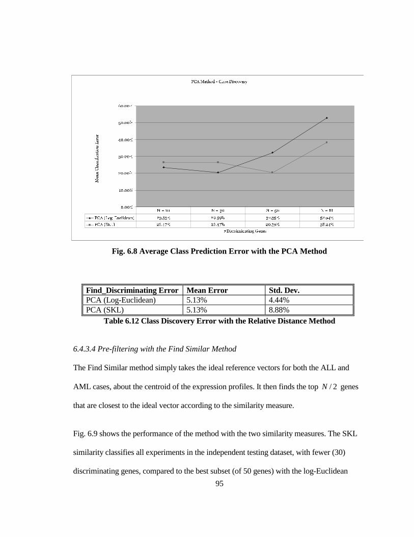
95
Fig. 6.8 Average Class Prediction Error with the PCA Method
Find_Discriminating Error Mean Error Std. Dev. PCA (Log-Euclidean) 5.13% 4.44% PCA (SKL) 5.13% 8.88%
Table 6.12 Class Discovery Error with the Relative Distance Method
6.4.3.4 Pre-filtering with the Find Similar Method
The Find Similar method simply takes the ideal reference vectors for both the ALL and
AML cases, about the centroid of the expression profiles. It then finds the top / 2N genes
that are closest to the ideal vector according to the similarity measure.
Fig. 6.9 shows the performance of the method with the two similarity measures. The SKL
similarity classifies all experiments in the independent testing dataset, with fewer (30)
discriminating genes, compared to the best subset (of 50 genes) with the log-Euclidean
PCA Method - Class Discovery
0.00%
10.00%
20.00%
30.00%
40.00%
50.00%
60.00%
#Discriminating Genes
Mean Classification Error
PCA (Log-Euclidean) 23.53% 20.59% 32.35% 52.94%
PCA (SKL) 26.47% 26.47% 20.59% 38.24%
N = 10 N = 30 N = 50 N = M
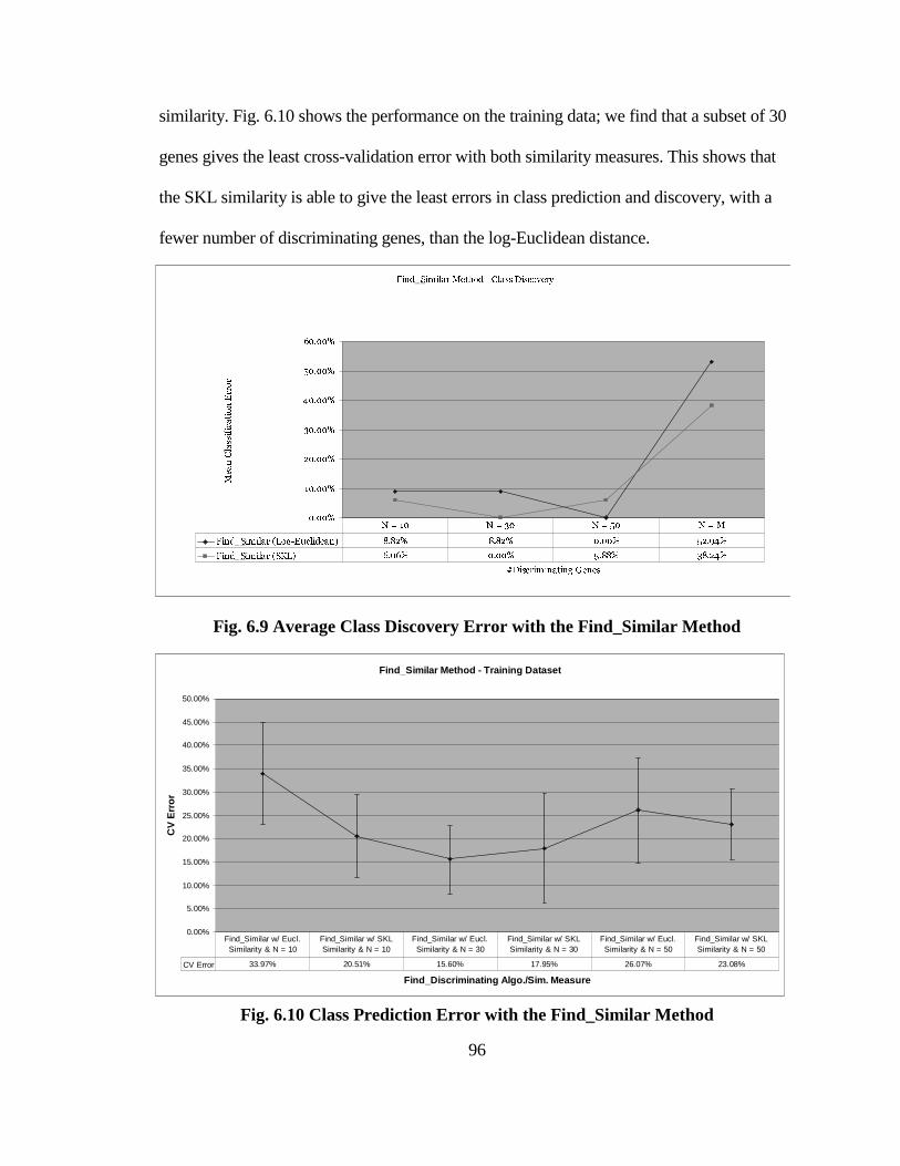
96
similarity. Fig. 6.10 shows the performance on the training data; we find that a subset of 30
genes gives the least cross-validation error with both similarity measures. This shows that
the SKL similarity is able to give the least errors in class prediction and discovery, with a
fewer number of discriminating genes, than the log-Euclidean distance.
Fig. 6.9 Average Class Discovery Error with the Find_Similar Method
Fig. 6.10 Class Prediction Error with the Find_Similar Method
Find_Similar Method - Class Discovery
0.00%
10.00%
20.00%
30.00%
40.00%
50.00%
60.00%
#Discriminating Genes
Mean Classification Error
Find_Similar (Log-Euclidean) 8.82% 8.82% 0.00% 52.94%
Find_Similar (SKL) 6.06% 0.00% 5.88% 38.24%
N = 10 N = 30 N = 50 N = M
Find_Similar Method - Training Dataset
0.00%
5.00%
10.00%
15.00%
20.00%
25.00%
30.00%
35.00%
40.00%
45.00%
50.00%
Find_Discriminating Algo./Sim. Measure
CV
Err
or
CV Error 33.97% 20.51% 15.60% 17.95% 26.07% 23.08%
Find_Similar w/ Eucl. Similarity & N = 10
Find_Similar w/ SKL Similarity & N = 10
Find_Similar w/ Eucl. Similarity & N = 30
Find_Similar w/ SKL Similarity & N = 30
Find_Similar w/ Eucl. Similarity & N = 50
Find_Similar w/ SKL Similarity & N = 50
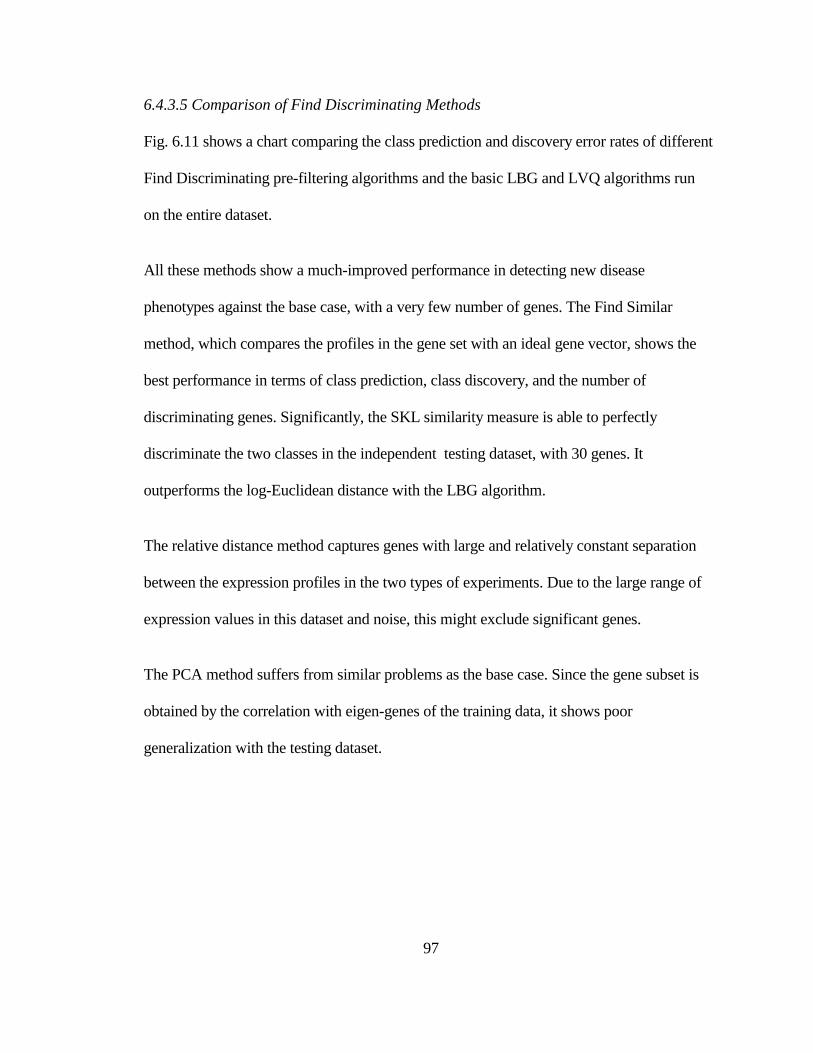
97
6.4.3.5 Comparison of Find Discriminating Methods
Fig. 6.11 shows a chart comparing the class prediction and discovery error rates of different
Find Discriminating pre-filtering algorithms and the basic LBG and LVQ algorithms run
on the entire dataset.
All these methods show a much-improved performance in detecting new disease
phenotypes against the base case, with a very few number of genes. The Find Similar
method, which compares the profiles in the gene set with an ideal gene vector, shows the
best performance in terms of class prediction, class discovery, and the number of
discriminating genes. Significantly, the SKL similarity measure is able to perfectly
discriminate the two classes in the independent testing dataset, with 30 genes. It
outperforms the log-Euclidean distance with the LBG algorithm.
The relative distance method captures genes with large and relatively constant separation
between the expression profiles in the two types of experiments. Due to the large range of
expression values in this dataset and noise, this might exclude significant genes.
The PCA method suffers from similar problems as the base case. Since the gene subset is
obtained by the correlation with eigen-genes of the training data, it shows poor
generalization with the testing dataset.
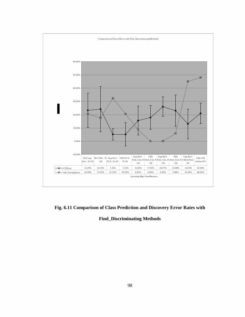
98
Fig. 6.11 Comparison of Class Prediction and Discovery Error Rates with
Find_Discriminating Methods
Compa rison of Ove ra ll Error wit h Find_Disc rimina t ing Me t hods
-10.00%
0.00%
10.00%
20.00%
30.00%
40.00%
50.00%
60.00%
Le a rning Algo/ S im Me a sure
CV Error 23.29% 24.15% 5.13% 5.13% 15.60% 17.95% 26.07% 23.08% 13.03% 20.94%
Ind. Te st ing Error 20.59% 17.65% 32.35% 20.59% 8.82% 0.00% 0.00% 5.88% 45.10% 48.04%
Re l. Log-
Euc l. , N = 50
Re l. S KL , N
= 50
Log-Euc l.
P CA , N = 50
S KL P CA ,
N = 50
Log-Euc l.
Find_S im ,N
= 30
S KL
Find_S im ,N
= 30
Log-Euc l.
Find_S im ,N
= 50
S KL
Find_S im ,N
= 50
Log-Euc l.
LVQ wit hout
P F
S KL LVQ
wit hout P F
99
6.5 Conclusions
In this thesis, we investigated processes in drug discovery through formal modeling
techniques from systems engineering. We built a UML use case model to capture the
requirements of a modern drug discovery analysis system and the related systems
integration issues. We developed system structure and behavior, and discussed alternate
methods of implementation. The discovery of efficient clustering algorithms for any
particular type of microarray data will lead to efficient indexing mechanisms over very
large experimental data sets. We also looked at database extensions that can handle new
data types and how they can be applied to biological data.
The next major focus of the thesis was the application of algorithms from signal processing
and machine learning, to the analysis of gene expression data. We investigated two
different types of analyses – functional and phenotypic classification, and found that the
supervised LVQ algorithm, with the LBG codebook initialization, shows very good
performance and is comparable to support vector machines, which are globally optimal
classifiers. We also applied an instance-based learning algorithm IB3, and found good
results with the identification of yeast functional classes.
We also described a novel similarity measure for clustering based on unnormalized
expression data, called the unnormalized symmetric Kullback-Liebler measure, based on
the concept of relative entropy, and originally developed in [24,25]. Though there was no
significant difference between the unnormalized SKL measure and log-Euclidean distance
with cDNA arrays (as expected), we found that the unnormalized SKL measure is able to
provide better performance with a leukemia oligonucleotide array data set. Different pre-
100
filtering methods for finding discriminating genes based on the Find Similar function,
PCA, relative distances, and the IB3 instance-based learning algorithm, were studied. All
methods except IB3 showed a large improvement in performance with pre-filtering. The
Find Similar pre-filtering method with the unnormalized SKL measure and the LBG/LVQ
algorithm together gave the best performance in class prediction and class discovery, with
the fewest number of discriminating genes.
101
BIBILIOGRAPHY
1. Alizadeh, A.A. et al. Distinct types of diffuse large B-cell lymphoma identified by
gene expression profiling. Nature 403, 503-511 (2000).
2. Brown, M.P. et al. Knowledge-based analysis of microarray gene expression data
by using support vector machines. Proc Natl Acad Sci USA 97, 262-267 (2000).
3. Cai, J. et al. Supervised Machine Learning Algorithms for Classification of Cancer
Tissue Types Using Microarray Gene Expression Data
<http://www.cpmc.columbia.edu/homepages/jic7001/cs4995/project1.htm>.
4. Eisen, M.B., Spellman, P.T., Brown, P.O. & Botstein, D., Cluster analysis and
display of genome-wide expression patterns. Proc Natl Acad Sci U S A 95, 14863-8
(1998).
5. Golub, T.R. et al. Molecular classification of cancer: class discovery and class
prediction by gene expression monitoring. Science 286, 531-7 (1999).
6. Duggan, D. J., Bittner, M., Chen, Y., Meltzer, P. & Trent, J. Expression Profiling
Using cDNA Microarrays. Nature Genetics 21, 10-14 (1999).
7. Lipschutz, R. J., Fodor, S. P. A., Gingeras, T. R. & Lockhart, D. J. High Density
Synthetic Oligonucleotide Arrays, Nature Genetics 21, 10-14 (1999).
8. Drug Target Validation and Identification of Secondary Drug Target Effects Using
DNA Microarrays; Matthew J. Marton, J. L. DeRisi, Holly A. Bennett, V. R. Iyer,
Michael R. Meyer, Christopher J. Roberts, Roland Stoughton, Julja Burchard,
David Slade, Hongyue Dai, Douglas E. Bassett Jr., Leland H. Hartwell, P. O.
Brown, and Stephen H. Friend; Nature Medicine 4:1293-1301 (1998).
102
9. Baldi, P., Brunak, S., Brunak, S. Bioinformatics: The Machine Learning Approach
(2nd Edition), MIT Press (2001).
10. Drlica, K. Understanding DNA and Gene Cloning: A Guide for the Curious (3rd
Edition), John Wiley & Sons (1996).
11. Cherkassky, V. S., Mulier, F. M., Learning from Data : Concepts, Theory, and
Methods, Wiley-Interscience (1998).
12. Cristianini, N., Shawe-Taylor, J., An Introduction to Support Vector Machines :
And Other Kernel-Based Learning Methods, Cambridge University Press (2000).
13. Aha, D., Kibler, D., Albert, M., Instance-based learning algorithms. Machine
Learning, 6:37--66, 1991.
14. Mitchell, T. M., Machine Learning, McGraw-Hill Higher Education (1997).
15. Gersho, A., Gray, R. M., Vector Quantization and Signal Compression, Kluwer
Academic Publishers (1992).
16. Kecman, V., Learning and Soft Computing, MIT Press (2001).
17. Baras, J. S., Dey, S., Combined Compression and Classification with Learning
Vector Quantization, IEEE Transactions on Information Theory, vol. 45, no. 6, pp.
1911-1920, September 1999.
18. Lavigna, A., Nonparametric Classification Using Learning Vector Quantization.
PhD thesis, Dept. of Electr. Eng., University of Maryland, College Park, Maryland
20742, 1989, ISR Technical Report PhD 90-1.
19. Linde, Y., Buzo, A., Gray, R. M., An Algorithm for Vector Quantization Design,
IEEE Trans. on Communication, pp. 702-710, 1980.

103
20. Hacia, J., Resequencing and Mutational Analysis using Oligonucleotide Arrays, ,
Nature Genetics 21, pp. 42-47 (1999).
21. Kohonen, T., Huang, T. S., Schroeder, M. R., Self-organizing Maps (3rd Edition),
Springer Verlag (2001).
22. Oliver, D. W., Kelliher, T. P., Keegan, J. G., Engineering Complex Systems with
Models and Objects, McGraw Hill (1997).
23. Dressman, M. A., Baras, A. S., Malinowski, R., Kwon, I., Walz, T.,
Polymeropoulos, M. H., Detecting Genes Amplification in Breast Cancer by
Combining Gene Expression Profiling and Gene Mapping, Submitted to Nature
Medicine, 2001.
24. Baras, A. S., Baras, J. S., A Novel Similarity Measure for Microarray Expression
Data, Submitted for publication, 2001.
25. Frankpitt, B., Baras, J. S., Baras, A. S., Yang, S., Analysis of Microarray Data,
Technical Report 2001-04B, AIMS, Inc., April 2001.
26. Barnes, L. M., Staedler, F. Liebman, J., Polymeropoulos, M. Laredan, C., Use of
Animal Samples to Study Human Diseases and Mechanisms of Drug Action by
Cross Species Hybridization of Human Microarrays, Am. J. Human Genetics,
69:462, Supplement 1, 2001.
27. Vinores, M., Polymeropoulos, M., Laredan, C., Gene Expression Mapping of
Various Regions of the Adult Human Brain, Am. J. Human Genetics, 69:453,
Supplement 1, 2001.
104
28. Baras, J. S., LaVigna, A., Convergence of Kohonen’s Learning Vector
Quantization, Prof. of the 1990 IJCNN Conference on Neural Networks, pp. 476-
482, San Diego, June 1990.
29. Kosmatopoulos, E., Christodoulou, M., Convergence Properties of a Class of
Learning Vector Quantization Algorithms, IEEE Trans. On Image Processing 5,
1996, pp. 366-388.
30. Cover, T. M., Thomas, J. A., Elements of Information Theory, Wiley-Interscience
(1991).
31. Ronan Collobert and Samy Bengio, SVMTorch: Support Vector Machines for
Large-Scale Regression Problems, Journal of Machine Learning Research, vol 1,
pages 143-160, 2001.
32. “Pharmaceutical Industry Profile 2000”, Pharmaceutical Research and
Manufacturers of America – Publications,
<http://www.phrma.org/publications/publications/profile00/>.
33. “How can we optimize selection of drug development candidates from many
compounds at the discovery stage?” Modern Drug Discovery, January/February
1999, 2(1), 55-60, <http://pubs.acs.org/hotartcl/mdd/99/janfeb/product.html>.
34. “The CDER Handbook”, The CDER Handbook,
<http://www.fda.gov/cder/handbook/>.
35. “New Drug Development Process”,
<http://www.kellogg.nwu.edu/faculty/radnor/htm/morsd56/website_readings/barbe
au_devtim.pdf>.

105
36. Sadoski, D., Two Tier Software Architectures,
<http://www.sei.cmu.edu/str/descriptions/twotier_body.html>.
37. Sadoski, D., Comella-Dorda, S., Three Tier Software Architectures,
<http://www.sei.cmu.edu/str/descriptions/threetier_body.html>.
38. Wallnau, K., Common Object Request Broker Architecture,
<http://www.sei.cmu.edu/str/descriptions/corba_body.html>.
