Impact Evaluation Report 28

Francisco Ceballos Isaac Manuel R Miguel Robles Andre Butler

Agriculture

Smallholder access to weather securities in India

Demand and impact on production decisions

August 2015

About 3ie

The International Initiative for Impact Evaluation (3ie) is an international grant-making NGO

promoting evidence-informed development policies and programmes. We are the global

leader in funding and producing high-quality evidence of what works, how, why and at what

cost. We believe that better and policy-relevant evidence will make development more

effective and improve people’s lives.

3ie Impact Evaluations

3ie-supported impact evaluations assess the difference a development intervention has

made to social and economic outcomes. 3ie is committed to funding rigorous evaluations

that include a theory-based design, use the most appropriate mix of methods to capture

outcomes and are useful in complex development contexts.

About this report

3ie accepted the final version of this report, Smallholder access to weather securities in

India: demand and impact on production decisions, as partial fulfilment of requirements

under grant OW2:103 issued under Open Window 2. The content has been copyedited and

formatted for publication by 3ie. Due to unavoidable constraints at the time of publication, a

few of the tables or figures may be less than optimal. All of the content is the sole

responsibility of the authors and does not represent the opinions of 3ie, its donors or its

Board of Commissioners. Any errors and omissions are also the sole responsibility of the

authors. All affiliations of the authors listed in the title page are those that were in effect at

the time the report was accepted. Any comments or queries should be directed to the

corresponding author, Miguel Robles at M.Robles@cgiar.org.

Funding for this impact evaluation was provided by 3ie’s donors, which include UKaid, the

Bill & Melinda Gates Foundation, Hewlett Foundation and 12 other 3ie members that provide

institutional support. A complete listing is provided on the 3ie website at

http://www.3ieimpact.org/en/about/3ie-affiliates/3ie-members/.

Suggested citation: Ceballos, Francisco, Manuel, R Isaac, Robles, Miguel, Butler, Andre,

2015, Smallholder access to weather securities in India: demand and impact on production

decisions, 3ie Grantee Final Report. New Delhi: International Initiative for Impact Evaluation

(3ie)

3ie Impact Evaluation Report Series executive editors: Jyotsna Puri and Beryl Leach

Managing editor: Omita Goyal

Assistant managing editors: Paromita Mukhopadhyay and Markus Olapade

Production manager: Pradeep Singh

Copy editor: Proteeti Banerjee

Cover design: John F McGill

Proofreader: Mathew PJ

Cover photo: Simon Chauvette

© International Initiative for Impact Evaluation (3ie), 2015

Smallholder access to weather securities in India: demand and

impact on production decisions

Francisco Ceballos

International Food Policy Research Institute

Isaac Manuel R

Institute for Financial Management and Research

Miguel Robles

International Food Policy Research Institute

Andre Butler

Institute for Financial Management and Research

3ie Impact Evaluation Report 28

August 2015

i

Acknowledgements

We take this opportunity to express our profound gratitude and deep regards to Ruth Hill

Vargas for her exemplary guidance in initiating this project and spearheading the research

with constructive inputs over the course of this project.

We thank Parendi Metha, Peter Ouzounov, Tirtha Chatterjee, Ashutosh Shekar, Ishani Desai

and Francisco Ceballos for their excellent research assistance on this project.

We are highly indebted to HDFC ERGO General Insurance Company for their support in

implementing this project. We express our sincere thanks to Priya Kumar, Azad Mishra and

Vivek Lalan for helping us in this project for the weather index insurance marketing and

management.

We would like to acknowledge Sharon Buteau for effectively managing the project

administration. Without her able guidance, this project would not have come to a successful

completion.

We express our deep sense of gratitude to International Initiative for Impact Evaluation (3ie),

International Food Policy Research Institute (IFPRI) and Institute for Financial Management

and Research (IFMR LEAD) for their financial aid and support in executing this research

project.

ii

Abstract

Weather-based insurance products insure farmers against production risks on the basis of a

weather index that is highly correlated to local yields. Indemnifications are triggered by pre-

specified patterns of the index, as opposed to actual yields. This eliminates the requirement

of on-field assessments for indemnification, thereby lowering administrative costs and time.

Therefore, index-based insurance products have been regarded as having enormous

potential to reach small farmers in developing countries. Surprisingly, the demand and take-

up rates are low for weather index insurance (WII) products. One of the reasons

hypothesised for the low demand and take-up of index-based insurance products is their

inherent complexity, which makes it difficult for farmers to perceive the direct benefits.

Hence, to encourage stronger participation, the project introduced an innovative WII product

that was simple, transparent, flexible and affordable for smallholder farmers. In fact, the

insurance product was a menu of very simple insurance options, each with a flat payment,

but different triggers and for different coverage periods. This product was tested in three

districts of Madhya Pradesh, India, during two consecutive summer agricultural seasons

(known as kharif in India) in 2011 and 2012 among the farmers who were cultivating rainfed

soya bean crop.

The main objective of this study was to assess the impact of the product (simplified WII) on

the production and consumption behaviours of smallholder farmers. In addition to this, the

research also investigated the responsiveness of insurance demand to a set of randomly

allocated interventions among farmers who were offered insurance products. These are:

1) Exogenous variation of the distance to the weather station by installing three new

weather stations, which were randomly positioned.

2) Random assignment of price discounts for the insurance offered.

3) Provision of training to all farmers being offered the insurance product, but random

variation of the intensity of training across villages.

A comparison of differences in outcome variables among the baseline and a follow-up

survey between control and treatment villages (through a difference in differences

estimation) provided us with a test of the impact of offering WII to smallholder farmers.

Empirically, we find evidence for the impact of our specific WII product, although results are

not strong, arguably due to a lack of power that arose because of low take-up of the product.

On the other hand, comparing take-up rates between different (randomly allocated)

treatment arms allowed us to evaluate the responsiveness of insurance demand to our

interventions, namely price discounts, weather station investments (a proxy to basis risk)

and intensive training on insurance literacy.

Overall, the demand for our simplified WII products was quite low, at 6.9 per cent and 4.03

per cent of the sample during kharif 2011 and 2012, respectively. We find that the demand

falls as price and distance to the weather station increase. On the other hand, the demand

for WII increases as product comprehension increases. Interestingly, the intensive insurance

literacy training sessions conducted in the first year seem to be of a more transient nature,

with no significant impact on understanding or demand during the second year. In terms of

the dynamic effects of the programme, while purchasing insurance does not have a

substantial impact on demand on its own in the subsequent year/season, purchasing

insurance and receiving a payout is strongly positively correlated with the decision to

iii

purchase insurance in the subsequent season. However, observing other households in the

village receiving a payout seems to have no impact on demand. This could also be

explained by the low levels of trust in the product or the insurance company. This is an

interesting avenue for future research.

The study seems to support the hypothesis that the purchase of WII could have influenced

the farmers to use hybrid seeds or high-yielding varieties to cultivate increased areas, to

cultivate new crops, to adopt improved cultivation practices and to get additional loans.

However, these results are not statistically strong.

The insights gained from the study enable us to propose the following policy

recommendations:

1) Thin networks of weather stations restrict the demand and scale-up of WII.

2) Provision of weather data by the weather service providers to the insurers has to

happen without any time lag to enable quick indemnification.

3) Distribution and marketing channels are key to enhance take-up and scale-up of WII

programmes.

4) An improved design of the WII product is key to minimise basis risk.

5) Affordability of WII insurance premiums is essential for a sustained take-up from

smallholder farmers.

6) One-time WII literacy programmes have little, if any, long-lasting impact on insurance

understanding and demand. This suggests that WII literacy programmes should be

designed as part of a more permanent process over time so they can contribute to

developing more sustainable micro-insurance markets (although more rigorous

evidence of this recommendation will require longer-term research projects than this

one).

iv

Contents Acknowledgements ............................................................................................................. i

Abstract ............................................................................................................................... ii

Abbreviations and acronyms ........................................................................................... vii

1. Introduction ..................................................................................................................... 1

2. Context ............................................................................................................................ 2

2.1 Background .................................................................................................................. 2

2.2 Related literature.......................................................................................................... 3

3. Intervention and theory of change ................................................................................. 5

3.1 Intervention .................................................................................................................. 5

3.2 Theory of change ......................................................................................................... 7

4. Implementation ............................................................................................................... 8

4.1 Designing of simplified weather index insurance products ......................................... 11

4.2 Marketing process ...................................................................................................... 12

4.3 Implementing premium subsidies ............................................................................... 13

4.4 Installing new weather stations .................................................................................. 14

4.5 Conducting insurance literacy training ........................................................................ 16

4.6 Data collection ........................................................................................................... 17

4.7 Weather shocks registered and the payouts made ..................................................... 19

5. Methodology: Randomisation and evaluation design ................................................ 20

5.1 Randomisation of insurance provision ........................................................................ 20

5.2 Randomisation of treatments ..................................................................................... 20

5.3 Selection of sample households ................................................................................. 21

5.4 Evaluation design....................................................................................................... 22

6. Impact analysis and results ......................................................................................... 23

6.1 Analysis of product take-up ........................................................................................ 23

6.2 Midline impact analysis .............................................................................................. 34

6.3 The longer run impact of offering insurance on demand............................................. 53

6.4 Endline qualitative assessment .................................................................................. 55

7. Triangulation of the results .......................................................................................... 64

7.1 Price discounts .......................................................................................................... 64

7.2 Insurance literacy training .......................................................................................... 64

7.3 Weather station .......................................................................................................... 65

7.4 Impact of the simplified weather index insurance on production and consumption

behaviours: ...................................................................................................................... 65

8. Conclusions and policy implications .......................................................................... 66

8.1 Conclusion ................................................................................................................. 66

8.2 Policy implications and recommendations: ................................................................. 69

Appendix ........................................................................................................................... 73

References ........................................................................................................................ 77

v

List of figures and tables

Figure 1: Theory of change ................................................................................................... 8

Figure 2: District map of Dewas, Bhopal and Ujjain ............................................................... 9

Figure 3: Project timeline .................................................................................................... 11

Figure 4: WII take-up pattern in kharif 2011 and kharif 2012 ............................................... 24

Figure 5: WII take-up pattern in kharif 2011 and kharif 2012 by household type.................. 24

Figure 6: Farmers’ preference for cheaper vs expensive WII contracts ............................... 25

Figure 7: Number of WII units purchased with reference to the premium subsidies ............. 26

Figure 8: Influence of insurance literacy training on take-ups .............................................. 26

Figure 9: Influence of new and old weather stations on WII take-up .................................... 27

Figure 10: WII take-up with reference to the distance from weather station ......................... 28

Figure 11: Households using other agriculture insurance products ..................................... 57

Figure 12: Awareness level of household about WBCIS ..................................................... 57

Figure 13: Reliability levels of weather station for farming households ................................ 58

Figure 14: Farmers’ expectations for the product’s payout .................................................. 59

Figure 15: Farmers’ opinion about the cost of the product ................................................... 60

Figure 16: Willingness to pay for simplified WII product ...................................................... 60

Table 1.1: Comparing treatment and control villages .......................................................... 10 Table 1.2: Product design ................................................................................................... 12 Table 1.3: Price discount allocations ................................................................................... 14 Table 1.4: Weather station assignment ……….. 15 Table 1.5: Comparing villages with insurance offered from new and old weather stations ... 16 Table 1.6: Balance between villages offering intense and basic insurance literacy training . 18 Table 1.7: Weather shocks registered and the payouts made ............................................. 19

Table 2.1: Randomisation of treatment villages into four categories .................................... 21

Table 2.2: Household types, based on education and landownership of household decision-

makers .............................................................................................................. 22

Table 3.1: Take-up among sampled households ................................................................. 30

Table 3.2: Log of area of land insured among sample households ...................................... 31

Table 3.3: Sample households, take-up (adding covariates) ............................................... 33

Table 3.4: Sample households, log of area insured (adding covariates) .............................. 33

Table 3.5: Minimum detectable effect of the comparison between average of treatment and

control in ANCOVA for ITT regressions ............................................................. 37

Table 3.6: Minimum detectable effect of the comparison between average of treatment and

control in ANCOVA for ATE regressions ........................................................... 38

Table 3.7: Impact of insurance on knowledge and trust ....................................................... 40

Table 3.8a: Specific OLS regression results of Impact of interventions on knowledge and

trust .................................................................................................................. 41

Table 3.8b: Specific IV 2SLS regression results of impact of interventions on knowledge and

trust .................................................................................................................. 41

Table 3. 9: Investigation into the effect of basic training ...................................................... 43

Table 3.10: Specific regression results of impact of intensive training, basis risk, and their

interaction ......................................................................................................... 44

Table 3.11: Specific regression results of impact of intensive training, voucher, and their

interaction ......................................................................................................... 44

vi

Table 3.12: Impact of insurance on kharif production .......................................................... 48

Table 3.13a: Impact of insurance on credit .......................................................................... 49

Table 3.13b: Impact of insurance on credit .......................................................................... 49

Table 3.14: Full regression results from the impact of offer and purchase of weather index

insurance on government insurance demand.................................................... 50

Table 3.15a: Impact of Insurance on transfers, employment and other sources of income .. 51

Table 3.15b: Impact of insurance on transfers, employment and other sources of income .. 52

Table 3.16: Take-up among sampled households, kharif 2012 ........................................... 54

Table 3.17: Take-up among households, kharif 2012, including price in kharif 2011 ........... 54

Table 3.18: Take-up among sampled households, kharif 2012, including uptake and payouts

in kharif 2011 .................................................................................................... 55

Table 3.19: Reason for non-purchase of insurance ............................................................. 56

Table 3.20: Factors influencing the take-up of WII with reference to weather station........... 58

Table 3.21: Farmers’ opinion about the WII product design ................................................ 59

Table 3.22: Farmers’ trust in the insurer .............................................................................. 61

Table 3.23: Reasons for not trusting the insurer .................................................................. 61

Table 3.24: Impact of WII on production behaviours of farmers ........................................... 62

Table 3.25: Influence of WII payout on production and consumption behaviours ................ 63

vii

Abbreviations and acronyms

ANCOVA analysis of covariance

ATE average treatment effect

FGD focus group discussion

HH

IFPRI

Household

International Food Policy Research Institute

IMD Indian Meteorological Department

IRDA Insurance Regulatory and Development Authority

ITT intent to treat

km kilometre

MDE minimum detectable effect

NAIS National Agricultural Insurance Scheme

WBCIS Weather Based Crop Insurance Scheme

WII weather index insurance

1

1. Introduction

Life for many farming households is risky. When this risk is uninsured, it poses a

considerable cost to current welfare as unfavourable events (such as weather shocks) will

reduce the production and consumption behaviours of agrarian livelihoods. Without

insurance, households take inefficient actions to limit their exposure to risk, and they may

pass up a profitable opportunity that is considered too risky1 or keep a high proportion of low

return/ high liquidity assets,2 which lower their average income.

Weather-based insurance products insure farmers against production risks on the basis of a

weather index (e.g. rainfall-based) that is theoretically correlated to local yields.

Indemnifications are triggered by pre-specified patterns of the index, as opposed to actual

yields (IFAD and WFP 2010). This eliminates the requirement of on-field assessments of

average yield for a given area, thereby lowering administrative costs and time. Therefore,

index-based insurance products have been regarded as having enormous potential to reach

small farmers in developing countries as they can stabilise farming production without

requiring farmers to make last resort sales of productive assets at a low price. Surprisingly,

the demand and take-up rates are low for weather index insurance products (Cole et al.

2012). One of the reasons hypothesised for the low demand and take-up of traditional index-

based insurance products is the inherent complexity of the products, which makes it difficult

for farmers to perceive the direct benefits (Gine et al. 2008).

Hence, to encourage stronger participation, the project introduced an innovative weather

index insurance (WII) product which was designed to address the scepticism and prejudices

of the farmers against traditional insurance schemes; it was simple, transparent, flexible and

affordable for smallholder farmers. This product was tested in three districts of Madhya

Pradesh, India, during two consecutive monsoon/summer seasons (known as kharif in India)

in 2011 and 2012.

The project evaluated the potential demand for this new WII product and its impact on the

production and consumption behaviours of farmers. The research also investigated the

barriers to the take-up of weather index insurance and also the responsiveness of insurance

demand to a set of interventions, namely price discounts, new and closer weather stations (a

proxy to basis risk) and training on insurance literacy.

Overall, our study found that the demand for the simplified WII products was quite low at 6.9

per cent and 4.03 per cent of the sample during kharif 2011 and 2012, respectively. We also

found that the demand falls as price and distance to the weather station increases. On the

other hand, the demand for WII increases as product comprehension increases.

Interestingly, our insurance literacy training intervention seems to be of a more transient

nature, with no significant impact on understanding or demand after the first year of its

implementation. It was also observed from the study that the purchase of WII has influenced

farmers to use hybrid seeds or high-yielding varieties to cultivate increased areas and new

crops, to adopt improved cultivation practices and to get additional loans. Although the study

1 Morduch (1991) finds that uninsured households grow low risk, low return crops. 2 In studies on the Indian poor, Rosenzweig and Binswanger (1993) find that uninsured households hold more

low-risk assets, and Fafchamps and Pender (1997) reported that they own more liquid (in unfavourable

circumstances) assets.

2

could find empirical evidence for the impact of WII, the results are not statistically strong due

to a lack of power because of low take-up of the product.

The remainder of the report narrates the methodology followed, the lessons learned and the

insights gained from the study. The paper is structured as follows: the next section contains

information on the study background and the current literature. Section 3 describes the

interventions in detail. Section 4 contains an overview of the programme implementation.

Section 5 states the randomisation method followed and the evaluation design adopted for

research. Section 6 presents the results of our take-up analysis, midline survey and

qualitative endline assessment. Section 7 briefly triangulates the results of our study, and

Section 8 provides the conclusion and policy recommendations.

2. Context

2.1 Background

India has 116 million operational farm holdings covering 163 million hectares with a vast

majority being small and marginal in size (approximately 80 per cent of farmers operate less

than 2 hectares), and a significant proportion of such households are below the poverty line

(World Bank and GFDRR 2011). Indian agriculture is heavily dependent on rainfall, which

largely occurs due to the seasonal winds that bring rains called the monsoon. The southwest

monsoon which coincides with kharif season (June–September) accounts for about 74 per

cent of the country’s total annual rainfall. It is the chief source of water supply for most of

peninsular India. In India, 60 per cent of the cropped area is under rainfed agriculture, which

produces 91 per cent of the coarse cereals, 90 per cent of pulses, 81 per cent of oilseeds,

65 per cent of cotton, 55 per cent of rice, and 25 per cent of wheat (Badatya 2005). Nearly

two thirds of the cropped acreage in India is vulnerable to drought in different degrees. On

an average, 12 million hectares of crop area are affected annually by natural disasters such

as drought, floods and cyclones, severely impacting the yields and total agricultural

production (GOI 2007). Normally, crop yield is influenced by the soil, topography, tillage

operations, and the use of inputs, namely seed, fertiliser, pesticides and irrigation, but it has

been established that in India, 50 per cent of the variations in crop yield is due to variations

in rainfall (Singh 2010). In this context, one can understand that agricultural risk

management products, particularly for the smallholder farmers, are of critical importance.

Weather risk is not a new phenomenon in India, and weather risk management in the broad

sense has long been practised. Farmers anticipate the rains using various indicators, and

time their planting and inputs based on their best estimates; they install irrigation systems if

they can and they reduce risk exposure by diversifying their livelihoods as far as possible

(Ellis 2000). Agricultural research has also sought ways to help manage the risk that weather

presents. However, variation in weather pattern is still affecting the economies of millions of

resource constrained marginal and small farmers in India. Evidence suggests that farmers

often sacrifice 10 to 20 per cent of income when using traditional risk management

strategies (e.g. borrowing, selling of assets and migration, among others (see Gautam et al.

1994). But if they can take up insurance, the picture may change.

3

In most areas of rural India, the only available formal insurance relating to agricultural

production is the public crop insurance scheme called National Agricultural Insurance

Scheme (NAIS). All farmers are required to purchase this insurance if they take a crop loan

from government banks. This rule introduces adverse selection in the insurance scheme, as

richer farmers (generally with lower production risk) are able to self-finance. On the other

hand, payout eligibility is based on crop damage assessments relative to experimental plots,

which requires a lot of resources and time. An evaluation of the traditional crop insurance

programme (NAIS) reveals that ‘while it has done well on equity grounds, the coverage and

indemnity payments are biased towards a few regions and crops, and there are delays in

settlement of claims’ (Nair 2010). In this scenario, WII was considered advantageous as it

insures against production risks on the basis of a weather index (e.g. rainfall) that is highly

correlated to local yields. Indemnifications are triggered by pre-specified thresholds for the

value of the index, as opposed to actual yield losses. This eliminates the requirement of on-

field assessments, thereby lowering administrative costs and time. Interestingly, the WII

sector in India has attracted private sector participation since 2002.

Nevertheless, despite a recent surge in interest among private companies and policymakers

in insuring farmers through weather index products, in practice, low demand and take-up

rates exist among farmers (Cole et al. 2012). One of the reasons hypothesised for the low

demand and take-up of the WII product is the inherent complexity, which makes it difficult for

farmers to perceive its direct benefits (Gine et al. 2008). To address this issue, this study

tested a very simple, transparent and flexible WII product. The product was launched

through a private insurance company called HDFC ERGO in the districts of Dewas, Bhopal

and Ujjain in the state of Madhya Pradesh, India, among smallholder farmers cultivating

rainfed soya bean crop during two consecutive summer agricultural seasons (kharif) in 2011

and 2012.

2.2 Related literature

A considerable amount of literature exists on the determinants of demand for index-based

products. We draw a number of hypotheses from this literature as to the likely determinants

of demand for index insurance (drawing on Hill, Hoddinott and Kumar 2011) to define

predictions about the likely impact of the price, basis risk and understanding on demand.

We start by considering a model of demand for WII following Clarke (2011), which assumes

well-informed individuals who make choices according to the expected utility theory.

Demand for weather insurance in this case will be a function of the price, the degree of basis

risk—the probability that the index triggers a payout different from the loss experienced by

the farmer3—and the degree to which an individual is risk averse. Since WII is not the same

as standard indemnity insurance, and in particular because these products contain basis

risk, demand for index products will be (under a minimal set of assumptions) decreasing in

basis risk and decreasing in the loading factor (the ratio of the price to the actuarially fair

price of the insurance contract). This means that installing a reference weather station closer

to a household’s farm should, by decreasing basis risk, increase demand for the index

product. Several studies analyse these questions and find results coherent with these

predictions (e.g. Gine et al. 2008; Mobarak and Rosenzweig, 2012; Karlan et al. 2012; Cole

et al. 2013). 3 Two extreme cases are: (i) The farmer experiences the largest possible yield loss and the insurance product

doesn’t trigger a payout; (ii) The farmer experiences no yield loss and the insurance product triggers the largest

possible payout.

4

Basis risk is a particularly critical problem in the context of index insurance. It arises due to

an index’s inadequacy to perfectly capture the individual losses of an insured farmer. This

imperfect relation can be related to a number of factors. First, the weather index may be

imperfectly measured because of the natural variation of weather between a measurement

station and the farmer’s plot. Second, a simple weather index cannot capture the full

complexity of the effect of weather on a crop, which might involve the interplay of a number

of weather variables (temperature, rainfall, humidity, evapotranspiration, winds), and on the

crop variety, soil quality and farming practices. Third, other non-weather events may impact

crop growth, such as pest attacks and diseases. Mobarak and Rosenzweig (2012) randomly

assign new weather stations to different Indian villages and find that demand for WII

decreases with distance to the weather station.

A critical feature of this model is the assumption of well-informed agents. However, weather

insurance is, for many, a new and unknown financial product. For some farmers, an

insurance purchase would represent the first time they engage with a formal financial

institution, and they may have some uncertainty about how this would work and how far such

an institution can be trusted. The benefits of the insurance contract itself may also not be

immediately clear, as there is much to learn about the probability distribution of rainfall at the

weather station, and the joint probability between rainfall at the weather station and a

farmer’s own yields. A farmer’s perception of the distribution of benefits may be highly

uncertain. As such, the decision of whether or not to purchase insurance is akin to the

decision to adopt a new technology (Gine et al. 2008; Lybbert et al. 2010). An example

consistent with this view is the tendency of farmers to purchase one or two units of

insurance—much less than would be required for full insurance—perhaps to experiment with

how well it works. This is similar to the observation that farmers experiment with new

technologies or practices on small portions of their land, as would be predicted by a

Bayesian model of learning about a new technology (Feder and O’Mara 1982; O’Mara 1971,

1980).

Competitively priced insurance that is designed to be risk reducing may not be perceived as

such as a result of uncertainty around returns and the probability that it will pay out when

needed. Consequently, although insurance is a financial product for which we would expect

demand to increase with risk aversion for some, if not all, of the distribution of risk

preferences, this relationship may not be observed. Technology adoption studies have long

reported that risk-averse households are less likely to be early adopters of new technologies.

Empirical analyses have shown that demand for insurance may decrease with risk aversion

across a range of high risk aversion (Gine, Townsend and Vickrey, 2007; Clarke and Kalani

2011; Gine et al. 2007; Hill, Hoddinott and Kumar 2011. This is also consistent with the

hypothesis that ambiguity aversion4 constrains insurance demand; Bryan (2010) has used

data collected in Malawi to test this hypothesis and finds evidence consistent with this

finding.

In addition to suggesting an alternate relationship between risk aversion and adoption,

conceptualising insurance as a technology adoption decision highlights the importance of

subjective expectations (Adesina and Baidu-Forson 1995), and thus the role of trust in

financial firms or the financial sector.

4 Ambiguity aversion pertains to the aversion towards the uncertainty about the probability distribution over

outcomes.

5

In this context of uncertain perceptions about the benefits and costs of index insurance,

increased training about risk management and insurance may help. If this training provides

farmers with an understanding that the benefits of insurance are higher than previously

understood, and a higher level of trust in the financial system that will provide them with the

insurance, farmers may increase their demand. However, it is also possible that training may

lead farmers to believe that the benefits of insurance are lower than they had previously

perceived, and as a result they may reduce their demand for insurance.

This point also relates to a strand of more recent empirical research focusing on the question

of whether observed realisations of insurance payouts serve the purpose of clearing some of

the uncertainty related to the adoption of new technology. In this hypothesis, observing a

payout may increase trust in the insurer and in the product, and even improve understanding

of the insurance product’s functioning. There are a few papers that have been able to

analyse the demand for index insurance over time (Cai, de Janvry and Sadoulet 2013;

Karlan et al. 2012; Cole, Stein and Tobacman 2014).

Finally, there are other factors that affect a farmer’s decision about whether or not to adopt a

new technology. A large body of literature shows that wealthier, more educated households

with entrepreneurial ability are more likely to be early adopters of new technologies (Feder,

Just and Zilberman 1985; Schultz 1981). We may expect similar relationships to be

observed among early adopters of WII (Gine et al. 2008). However, weather insurance will

be but one element in households’ portfolio of risk management activities. Others include

actions that ex-ante smooth income—such as diversifying into livestock or off-farm

activities—and actions to smooth consumption, such as savings and borrowing, transfers

within networks to spread risk, and accumulation and decumulation of physical assets.

Households with good networks and access to savings and borrowing instruments may have

a lower demand for insurance than those without access to these activities, if the cost of

engaging in these activities is lower than the cost of purchasing insurance, if it reduces

consumption variability and if insurance is perceived as a substitute for these. The demand

for WII will increase with the presence of these risk management activities where it is seen to

complement existing mechanisms (Mobarak and Rosenzweig 2012).

3. Intervention and theory of change

3.1 Intervention

The primary intervention of this project was the provision of simplified weather securities

(simple weather-indexed insurance products) to smallholder farmers in three districts of

Dewas, Bhopal and Ujjain in the state of Madhya Pradesh, India. These WII were sold

through an insurance company named HDFC ERGO. Randomly selected farmers were

given the option to purchase the simplified WII from HDFC ERGO. These WII are innovative

weather-index insurance products designed by IFPRI to be simple, transparent, flexible and

affordable for smallholder farmers. (The details of this simple weather-indexed insurance

product and its implementation process are elaborated in Section 4 and Appendix A.)

In addition to this, the project also had three other interventions: (i) variation in the provision

of insurance literacy training programmes; (ii) installation of new reference weather stations

in randomly selected locations; and (iii) provision of different premium subsidies. These

interventions are mainly to assess its impact in take-up behaviour by the farmers. (The

details of these interventions are presented in Section 4.)

6

With these interventions, the study intended to test the impact of having access to WII on the

production and consumption behaviours of smallholder farmers. In particular, the study

aimed at shedding light on some of the following questions: Do farmers switch to higher

return technologies once risk is accounted for? Does their consumption pattern change in

response to changes in their expected income flows? In addition, another objective of the

study was to assess the determinants of product take-up by smallholder farmers. In

particular, it intended to analyse the extent and importance of commonly cited demand

obstacles, such as affordability of the insurance instrument, understanding of the insurance

product and farmers’ perception of the implicit geographic basis risk in index products.

3.1.1 The product

Weather index insurance products insure farmers against production risks on the basis of a

weather index (e.g. rainfall). The weather index serves as a proxy for losses rather than the

assessed losses of each individual policyholder. This eliminates in-field assessments of

average yield for a given area, thereby lowering administrative costs. The key advantage of

WII for the farmers is that indemnity payments get settled quickly because of no in-field

assessment, and because transaction costs get lower for insurers, these reduced costs

should generally be passed along to farmers themselves. In theory, at least, this makes WII

financially viable for private sector insurers and the product becomes more affordable to

small farmers.

Weather index insurance products have been marketed in India from 2003 onwards, but the

take-up rates have been low (Cole et al. 2012). One of the reasons hypothesised for the low

demand and take-up of WII has been the inherent complexity of the products, which makes it

difficult for farmers to assess the real benefits (Gine et al. 2008). For example, in a WII

contract for deficit rainfall, a farmer should be aware of and be able to broadly calculate the

levels of rainfall deficit that affect his crops at different crop stages, an estimation of the

ultimate impact of this deficit rainfall in terms of crop losses, and the correlation between

rainfall at his plot and the weather station. It involves non-trivial calculations to make

informed decisions about the product, which makes it complex and difficult for the farmers to

understand WII.

In addition, WII products have traditionally been designed as fixed contracts with a specific

payout function related to the hypothesised losses of an average farmer in the region. This

type of contract generally offers a linear payout function after a certain trigger, which

depends on the difference between the recorded value of the index and the trigger point.

This makes the product even more difficult to understand, and takes away any flexibility for

adapting the product to the heterogeneity of crops and farming practices in the region.

Hence, under the hypothesis that a simple WII product may lead to better understanding by

the farmers and ultimately increase take-up rates, the project introduced an innovative

simple WII product that does not involve complex calculations to estimate payouts. Instead,

this product triggers a flat payment if the weather index is above a single trigger, and nothing

otherwise.

7

Moreover, the simplified WII product included a small portfolio of different insurance

contracts for different periods instead of a single WII contract for the entire crop period. In

particular, the crop growth period was split into three phases (cover periods) of shorter

duration, and simplified WII contracts were offered for each phase so as to enable payouts

immediately after the lapse of a phase.

For each of these cover periods, there were two types of simplified WII contracts offered.

One WII contract was intended to pay on the occurrence of a very low probability event

representing severe yield losses (e.g. extreme deficit or excess rainfall from the optimal

level; the probability of occurrence of these events is very rare and they can cause severe

damages to crops). The other contract was intended to pay on the occurrence of a

moderately probable event (e.g. slight deficit or excess rainfall from the optimal level; these

events may occur occasionally and their impact on crop growth would be moderately

detrimental). By offering products for different weather (rainfall) risk levels, we allowed

farmers to choose an insurance portfolio suited to their specific combination of extreme and

moderate risk. In sum, we designed very simple contracts for different coverage periods and

risks levels and gave farmers the option to freely choose a combination of them.

3.2 Theory of change

The theory of change underlying this experiment is presented in Figure 1.

Purchase decisions of WII depend on a number of farmer-level factors, which will be the

main focus of this report. Among these, we can mention product understanding, affordability

(price), basis risk, trust in the insurer and availability of other risk management options. By

simplifying the product, as explained in the previous section, our project intends to remove

some aspects of the above complexities. More specifically, we speculate that this new type

of index insurance will result in easier understanding by farmers with low levels of literacy,

which will also contribute to enhancing trust in the insurer. Moreover, through the installation

of new weather stations, the average distance to the farmer’s plot will be (exogenously)

reduced, which will encourage insurance uptake. These channels have the potential to be

successful in strengthening demand.

Now, uptake of WII by a farmer may influence him to invest more in his farming operation by

both reducing his perceived levels of risk and by mitigating current credit constraints. Both

these effects would have a positive impact in terms of investment in agricultural inputs by, for

example, applying higher yielding varieties or hybrid seeds, or by encouraging the farmer to

increase the area of cultivation. This could, in turn, result in a feedback loop through which

more formal credits may become available.

If the risks were not to materialise, the above investments should directly impact the farmer’s

welfare through increased crop yields and a boost in farm income. Moreover, the latter

should also have a direct bearing on consumption behaviours, both in terms of quantity and

quality. Under the worst case scenario of the realisation of these weather risks, holding

insurance against these would then enable the farmer to start a new production cycle or to

cover his losses in the current production cycle with fewer difficulties.

8

4. Implementation

According to our original project plan, we have aimed to implement the project in two states

of India, namely Karnataka and Madhya Pradesh, during the cropping season kharif 2011.

These two states presented different on-the-ground research environments. Karnataka was

of great interest for the project because it is a state where the government subsidises index

Figure 1: Theory of change

9

insurance. However, we learned that access to subsidies can occur only under two

situations: (i) bundled credit insurance programme, in which insurance is mandatory, and (ii)

as a stand-alone product, but in which the insurance product is designed as approved by the

government. In Madhya Pradesh, there was freedom to design innovative products without

having to compete with state insurance products bundled with government credit. According

to this original plan, 180 villages were to be selected (90 villages in each state). Weather

index insurance was to be offered in 120 of these villages, selected randomly, whilst

individuals in the remaining 60 villages would form the control group. But we decided not to

implement the project according to this original plan since the state government of Karnataka

was not able to offer subsidies for our simplified WII product as they were subsidising only

the traditional WII product. Since the design of this traditional product runs counter to our

project objectives of providing simple, transparent and flexible weather securities, and also

considering the limited chance of our product to compete with the subsidised government

product, we have ultimately dropped the implementation of the project in the state of

Karnataka. Given this limitation, we were ratified by 3ie to implement the project in the state

of Madhya Pradesh alone for two cropping seasons, i.e. kharif 2011 and kharif 2012, by

increasing the number of villages from 90 to 110.

In accordance with this, the study was

implemented in the districts of Dewas

and Bhopal, with the inclusion of an

additional district, Ujjain, to

accommodate the increased number of

villages for implementation in Madhya

Pradesh among the smallholder farmers

cultivating rainfed soya bean crop. The

districts were selected according to a

number of different qualitative factors

assessed during the design stage

between the project team, the insurance

company and local officials. Among these factors are the high rainfall risk these districts

faced, coupled with the fact that they included a large number of smallholder farmers

growing rainfed soya bean, the fact that these districts had not yet been notified by the

government for its subsidised agricultural insurance scheme, and the availability of historical

rainfall data to be used for product design. We worked with the insurance company HDFC

ERGO to identify suitable villages to be included in the study. Suitable villages were defined

as those that were 15 to 20 kilometres or less from a reference weather station, and those in

which HDFC ERGO had a marketing presence. Additionally, it was important to select

villages that were neither too small nor too large for surveying and marketing activities.

First, administrative data on the number of households within a village were used to exclude

villages of less than 100 households and more than 500 households. This resulted in a list of

about 120 villages in three districts. Second, 45 villages in Dewas and Bhopal and 20

villages in Ujjain, 110 villages in total, were randomly selected for inclusion in this study. In

each village, 30 households were sampled for study purposes. Seventy-two out of 110

villages were selected at random (30 in Bhopal, 29 in Devas and 13 in Ujjain) and WII was

offered to the sampled households in these treatment villages, while households in the

Figure 2: District map of Dewas, Bhopal and Ujjain

10

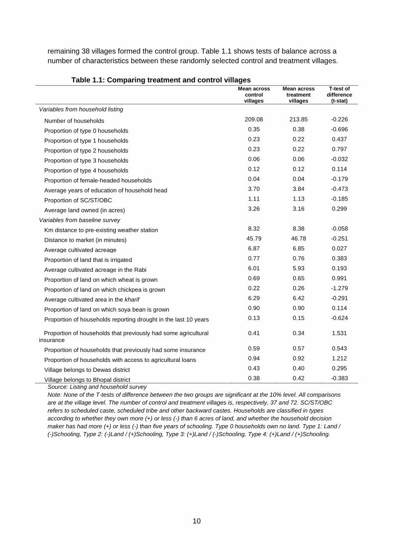
remaining 38 villages formed the control group. Table 1.1 shows tests of balance across a

number of characteristics between these randomly selected control and treatment villages.

Table 1.1: Comparing treatment and control villages

Mean across control villages

Mean across treatment villages

T-test of difference

(t-stat)

Variables from household listing

Number of households 209.08 213.85 -0.226

Proportion of type 0 households 0.35 0.38 -0.696

Proportion of type 1 households 0.23 0.22 0.437

Proportion of type 2 households 0.23 0.22 0.797

Proportion of type 3 households 0.06 0.06 -0.032

Proportion of type 4 households 0.12 0.12 0.114

Proportion of female-headed households 0.04 0.04 -0.179

Average years of education of household head 3.70 3.84 -0.473

Proportion of SC/ST/OBC 1.11 1.13 -0.185

Average land owned (in acres) 3.26 3.16 0.299

Variables from baseline survey

Km distance to pre-existing weather station 8.32 8.38 -0.058

Distance to market (in minutes) 45.79 46.78 -0.251

Average cultivated acreage 6.87 6.85 0.027

Proportion of land that is irrigated 0.77 0.76 0.383

Average cultivated acreage in the Rabi 6.01 5.93 0.193

Proportion of land on which wheat is grown 0.69 0.65 0.991

Proportion of land on which chickpea is grown 0.22 0.26 -1.279

Average cultivated area in the kharif 6.29 6.42 -0.291

Proportion of land on which soya bean is grown 0.90 0.90 0.114

Proportion of households reporting drought in the last 10 years 0.13 0.15 -0.624

Proportion of households that previously had some agricultural insurance

0.41 0.34 1.531

Proportion of households that previously had some insurance 0.59 0.57 0.543

Proportion of households with access to agricultural loans 0.94 0.92 1.212

Village belongs to Dewas district 0.43 0.40 0.295

Village belongs to Bhopal district 0.38 0.42 -0.383

Source: Listing and household survey

Note: None of the T-tests of difference between the two groups are significant at the 10% level. All comparisons

are at the village level. The number of control and treatment villages is, respectively, 37 and 72. SC/ST/OBC

refers to scheduled caste, scheduled tribe and other backward castes. Households are classified in types

according to whether they own more (+) or less (-) than 6 acres of land, and whether the household decision

maker has had more (+) or less (-) than five years of schooling. Type 0 households own no land. Type 1: Land /

(-)Schooling, Type 2: (-)Land / (+)Schooling, Type 3: (+)Land / (-)Schooling, Type 4: (+)Land / (+)Schooling.

11

Before the initiation of the project, during kharif 2010 we did a pilot testing of our new

simplified WII product in three villages, namely Banedia, Chander and Khajraya of Depalpur

tehsil of Indore district in Madhya Pradesh. The main objective of this pilot was to test our

simplified WII product design in a real case scenario and not to study the impact of the

product on the farmer’s livelihood. The learning from this pilot test was carried forward in

designing the WII products during the cropping seasons of kharif 2011 and kharif 2012. We

have implemented all the project interventions like conducting insurance literacy training

programmes, installation of new weather stations and provision of premium subsidies well

before the start of the first cropping season, kharif 2011. All the data collection activities like

executing a listing exercise, a baseline survey, midline survey and an endline survey were

done in stipulated times. This is clearly depicted in the timeline of the project presented in

Figure 3, and the details of the implementation of each project activity are elaborated below.

4.1 Designing of simplified WII products

The project introduced an innovative simple WII product with a flat and easy to understand

payout if the event (weather index) written on it comes true. A traditional WII product

involves some calculation to determine the payout amount, which makes the product

complex and difficult for farmers to understand. Moreover, the simplified WII offered provided

a menu of options among different simple insurance contracts. Instead of offering one WII

contract covering the entire crop period, we offered WII contracts for shorter periods. Here,

the entire crop growth period was split into three phases (cover periods) of shorter duration

and simplified WII contracts were offered for each phase so as to enable payouts

immediately after the lapse of a phase to enable the farmer to take corrective action.

Focus group discussions (FGDs) were conducted in selected villages from the three districts

of Devas, Bhopal and Ujjain. They provided information for the design of our product.

Discussions with farmers enabled us to understand the perils faced by their crops, the critical

periods of rainfall and the approximate crop losses during these periods. These perils, their

duration and the average losses were similar across the three districts. On the basis of this

Figure 3: Project timeline

12

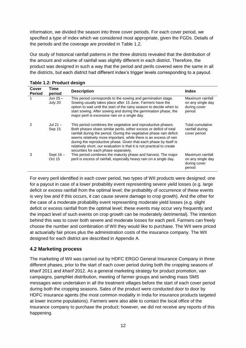
information, we divided the season into three cover periods. For each cover period, we

specified a type of index which we considered most appropriate, given the FGDs. Details of

the periods and the coverage are provided in Table 1.2.

Our study of historical rainfall patterns in the three districts revealed that the distribution of

the amount and volume of rainfall was slightly different in each district. Therefore, the

product was designed in such a way that the period and perils covered were the same in all

the districts, but each district had different index’s trigger levels corresponding to a payout.

Table 1.2: Product design

Cover Period

Time period

Description Index

1 Jun 25 – July 20

This period corresponds to the sowing and germination stage. Sowing usually takes place after 15 June. Farmers have the option to wait until the start of the rainy season to decide when to start sowing. After sowing and during the germination phase, the major peril is excessive rain on a single day.

Maximum rainfall on any single day during cover period

2 Jul 21 – Sep 15

This period combines the vegetative and reproductive phases. Both phases share similar perils, either excess or deficit of total rainfall during the period. During the vegetative phase rain deficit seems relatively more important, while there is an excess of rain during the reproductive phase. Given that each phase by itself is relatively short, our evaluation is that it is not practical to create securities for each phase separately.

Total cumulative rainfall during cover period

3 Sept 16 – Oct 15

This period combines the maturity phase and harvest. The major peril is excess of rainfall, especially heavy rain on a single day.

Maximum rainfall on any single day during cover period

For every peril identified in each cover period, two types of WII products were designed: one

for a payout in case of a lower probability event representing severe yield losses (e.g. large

deficit or excess rainfall from the optimal level; the probability of occurrence of these events

is very low and if this occurs, it can cause severe damage to crop growth). And the other for

the case of a moderate probability event representing moderate yield losses (e.g. slight

deficit or excess rainfall from the optimal level; these events may occur very frequently and

the impact level of such events on crop growth can be moderately detrimental). The intention

behind this was to cover both severe and moderate losses for each peril. Farmers can freely

choose the number and combination of WII they would like to purchase. The WII were priced

at actuarially fair prices plus the administration costs of the insurance company. The WII

designed for each district are described in Appendix A.

4.2 Marketing process

The marketing of WII was carried out by HDFC ERGO General Insurance Company in three

different phases, prior to the start of each cover period during both the cropping seasons of

kharif 2011 and kharif 2012. As a general marketing strategy for product promotion, van

campaigns, pamphlet distribution, meeting of farmer groups and sending mass SMS

messages were undertaken in all the treatment villages before the start of each cover period

during both the cropping seasons. Sales of the product were conducted door to door by

HDFC insurance agents (the most common modality in India for insurance products targeted

at lower income populations). Farmers were also able to contact the local office of the

insurance company to purchase the product; however, we did not receive any reports of this

happening.

13

In Dewas and Bhopal during kharif 2011, the WII were sold only for the second and third

cover periods, because during the first cover period the insurance company HDFC ERGO

utilised its entire market force to sell other government insurance products in the

neighbouring districts. In Ujjain, WII were marketed only for the third cover period during

kharif 2011 as the household survey of this additional district was completed during the

second cover period. This delay in Ujjain was because of its delayed inclusion in the project

to increase the number of villages, as we could not implement our project in Karnataka state.

Considering the issues of no marketing during the first phase and the inclusion of additional

villages in Ujjain at a later stage, HDFC agents were instructed to perform door to door visits

for the entire household sample during the marketing phase, and were provided with

monetary incentives for each sale they brought in.

Low take-up rates were a concern during the kharif 2011 season and it was not clear from

the midline data how much of this was due to a lack of information about the products.

Consequently, we worked with HDFC ERGO to design a comprehensive marketing strategy

for kharif 2012. To ensure that there were no capacity constraints in implementing the

marketing activities (particularly the door to door sales), we hired a field-level organisation

named Sigma Research and Consulting to do the door to door sales of WII on behalf of

HDFC ERGO. Sigma’s field staff were trained by HDFC ERGO to sell the WII product of this

study.

4.3 Implementing premium subsidies

Exogenous variation in the price of the insurance products was introduced by randomly

allocating price discount vouchers among treatment households. Inducing exogenous

variation in the price of insurance allows us to understand and measure how insurance

demand responds to price changes or, in other words, the demand price elasticity. Following

a standard law of demand, our hypothesis was that holding constant other factors that might

affect demand, the demand for insurance products is decreasing (or not increasing) in

prices.

Discounts were introduced in absolute terms. Based on group discussions and given the

level of education of targeted farmers, we concluded that absolute numbers would be more

easily understood by farmers rather than percentage discounts. Four levels of discounts

were selected to make them close to 15 per cent, 30 per cent, 45 per cent and 60 per cent

price discounts, so that we have enough price variation along a hypothetical demand curve.

In Dewas and Bhopal districts during kharif 2011, the following four levels of discounts were

allocated: ₹45, ₹90, ₹135 and ₹180.5 Out of the 30 sampled households in a village, five

households received a discount voucher for ₹45, five households received a discount

voucher for ₹90, five households received a discount voucher for ₹135, five households

received a discount voucher for ₹180 and 10 households did not received any discount

vouchers. All non-sampled households in treatment villages received no discount. The

lottery method was used in distributing the households with the subsidy vouchers. The

HDFC insurance company decided to have a more aggressive pricing policy in Ujjain (low

loading and therefore lower prices), which was included at a later stage in the third cover

5 The market price of the product without a discount was between ₹200 to ₹350; see Appendix A.

14

period, and so the discounts offered in Ujjain were adjusted accordingly. In Ujjain district, the

discount levels were ₹30, ₹60, ₹90 and ₹120. The distribution of different levels of price

subsidies within the villages created farmer dissatisfaction and provoked prejudices which, in

turn, affected the marketing process in Dewas and Bhopal. Considering these difficulties, the

protocol for discount distribution in Ujjain was later modified. In Ujjain, all households

(sampled and non-sampled) in treatment villages were assigned one of the following

discounts: of ₹0, 30, 60, 90 and 120. Out of the 13 selected treatment villages, two villages

were given a discount of ₹30, two were given a discount of ₹60, two were given a discount of

₹90, two were given a discount of ₹120, and five villages did not receive any discount.

During kharif 2012, unlike kharif 2011, uniform village-wise premium discounts were given by

randomly assigning all the treatment villages with one of the following discounts: of ₹0, ₹40,

₹75, ₹115 and ₹150.

Table 1.3: Price discount allocations

kharif 2011 kharif 2012

Bhopal and Dewas treatment villages

Ujjain treatment villages

Bhopal, Dewas and Ujjain treatment villages

Premium discount allocation method followed

Random at the household level

Random at the village level

Random at the village level

Value of discount allocated

₹0: 10 sampled households and all the non-sampled households ₹45: 5 sampled households ₹90: 5 sampled households ₹135: 5 sampled households ₹180: 5 sampled households

₹0: all households in 5 villages ₹30: all households in 2 villages ₹60: all households in 2 villages ₹90: all households in 2 villages ₹120: all households in 2 villages

₹0: 6 treatment villages each in Dewas and Bhopal; 5 treatment villages in Ujjain ₹40: 6 treatment villages each in Dewas and Bhopal; 2 treatment villages in Ujjain ₹75: 6 treatment villages each in Dewas and Bhopal; 2 treatment villages in Ujjain ₹115: 6 treatment villages each in Dewas and Bhopal; 2 treatment villages in Ujjain ₹150: 6 treatment villages Bhopal, 5 treatment villages in Dewas and 2 treatment villages in Ujjain

4.4 Installing new weather stations

Proximity of weather stations to a farmer’s field is a prerequisite for a successful weather

index-based product. As distance to the weather station increases, the difference between

rain on a farmer’s field and rain recorded at the weather station also increases, and as a

result, so does the degree of risk that is not covered (basis risk). Individuals facing higher

basis risk are less likely to purchase WII; and when they do purchase it, these WII will be

less beneficial to their production decisions and welfare.

15

In practice, assessing the impact of basis risk is difficult as weather stations are not

exogenously located but are often located close to markets, municipal centres and other

endogenous landmarks. To study the impact of basis risk, distance to the weather station

was exogenously varied by installing three new randomly located weather stations among

the treated villages.

The locations of the new weather stations were randomly selected in order to ensure

similarity in the average characteristics between treatment villages that are to be served by a

new weather station, and those that would be served by an existing weather station. In

particular, three new weather stations were installed in locations selected using the following

process:

(1) We excluded all treatment villages at 5 kilometres or less from an existing

weather station. Out of the non-excluded treatment villages, we randomly

selected one village in which to place a new weather station. All villages very

close (5 kilometres or less) to this one were then excluded from further selection.

(2) Out of the remaining villages, we randomly selected a second location. All

villages very close (5 kilometres or less) to this one were then excluded from

further selection.

(3) Out of the remaining villages, we randomly selected a third location.

The three villages selected for new station installations using this process were Polayjagir

and Talod in Dewas, and Intkhedi Sadak in Bhopal. Thirty treatment villages were then

assigned to a new weather station based on closest proximity, and the remaining 42 villages

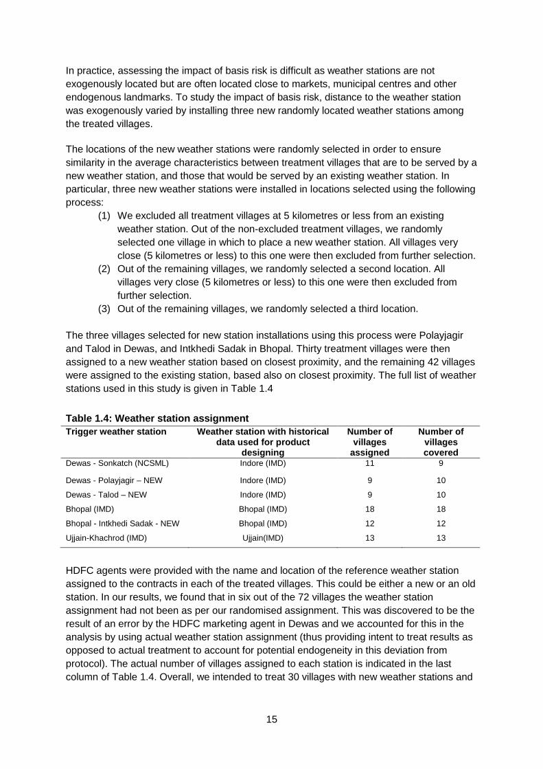
were assigned to the existing station, based also on closest proximity. The full list of weather

stations used in this study is given in Table 1.4

Table 1.4: Weather station assignment

Trigger weather station Weather station with historical data used for product

designing

Number of villages

assigned

Number of villages covered

Dewas - Sonkatch (NCSML) Indore (IMD) 11 9

Dewas - Polayjagir – NEW Indore (IMD) 9 10

Dewas - Talod – NEW Indore (IMD) 9 10

Bhopal (IMD) Bhopal (IMD) 18 18

Bhopal - Intkhedi Sadak - NEW Bhopal (IMD) 12 12

Ujjain-Khachrod (IMD) Ujjain(IMD) 13 13

HDFC agents were provided with the name and location of the reference weather station

assigned to the contracts in each of the treated villages. This could be either a new or an old

station. In our results, we found that in six out of the 72 villages the weather station

assignment had not been as per our randomised assignment. This was discovered to be the

result of an error by the HDFC marketing agent in Dewas and we accounted for this in the

analysis by using actual weather station assignment (thus providing intent to treat results as

opposed to actual treatment to account for potential endogeneity in this deviation from

protocol). The actual number of villages assigned to each station is indicated in the last

column of Table 1.4. Overall, we intended to treat 30 villages with new weather stations and

16

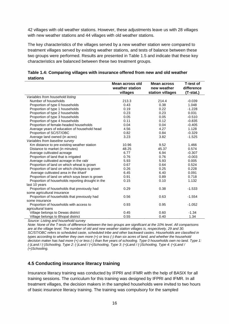
42 villages with old weather stations. However, these adjustments leave us with 28 villages

with new weather stations and 44 villages with old weather stations.

The key characteristics of the villages served by a new weather station were compared to

treatment villages served by existing weather stations, and tests of balance between these

two groups were performed. Results are presented in Table 1.5 and indicate that these key

characteristics are balanced between these two treatment groups.

Table 1.4: Comparing villages with insurance offered from new and old weather

stations

Mean across old weather station

villages

Mean across new weather

station villages

T-test of difference (T-stat.)

Variables from household listing

Number of households 213.3 214.4 -0.039 Proportion of type 0 households 0.43 0.38 1.048 Proportion of type 1 households 0.19 0.22 -1.228 Proportion of type 2 households 0.23 0.23 0.031 Proportion of type 3 households 0.05 0.05 -0.510 Proportion of type 4 households 0.11 0.12 -0.835 Proportion of female-headed households 0.04 0.04 -0.405 Average years of education of household head 4.56 4.27 1.128 Proportion of SC/ST/OBC 0.82 0.84 -0.329 Average land owned (in acres) 3.23 3.82 -1.525

Variables from baseline survey Km distance to pre-existing weather station 10.96 9.52 1.466 Distance to market (in minutes) 48.25 45.37 0.574 Average cultivated acreage 6.77 6.94 -0.307 Proportion of land that is irrigated 0.76 0.76 -0.003 Average cultivated acreage in the rabi 5.93 5.93 0.005 Proportion of land on which wheat is grown 0.67 0.64 0.524 Proportion of land on which chickpea is grown 0.26 0.25 0.228 Average cultivated area in the kharif 6.45 6.40 0.091 Proportion of land on which soya bean is grown 0.91 0.89 0.718 Proportion of households reporting drought in the

last 10 years 0.15 0.10 1.132

Proportion of households that previously had some agricultural insurance

0.29 0.38 -1.533

Proportion of households that previously had some insurance

0.56 0.63 -1.554

Proportion of households with access to agricultural loans

0.93 0.95 -1.052

Village belongs to Dewas district 0.45 0.60 -1.34 Village belongs to Bhopal district 0.55 0.40 1.34

Source: Listing and household survey Note: None of the T-tests of difference between the two groups are significant at the 10% level. All comparisons are at the village level. The number of old and new weather station villages is, respectively, 29 and 30. SC/ST/OBC refers to scheduled caste, scheduled tribe and other backward castes. Households are classified in types according to whether they own more (+) or less (-) than six acres of land, and whether the household decision maker has had more (+) or less (-) than five years of schooling. Type 0 households own no land. Type 1: (-)Land / (-)Schooling, Type 2: (-)Land / (+)Schooling, Type 3: (+)Land / (-)Schooling, Type 4: (+)Land / (+)Schooling.

4.5 Conducting insurance literacy training

Insurance literacy training was conducted by IFPRI and IFMR with the help of BASIX for all

training sessions. The curriculum for this training was designed by IFPRI and IFMR. In all

treatment villages, the decision makers in the sampled households were invited to two hours

of basic insurance literacy training. The training was compulsory for the sampled

17

households. If the decision maker could not attend, some other representative for the

household had to attend; in this way we ensured the complete participation of sampled

households. In these basic training sessions, which were also open to any other observers

from the village, farmers were first introduced to the various weather-related risks that they

might face and were encouraged to discuss their pre-existing coping mechanisms. After this

introduction, the bulk of the remaining training focused on a general discussion of WII, how it

has been tailored for their circumstances and the specifics of the product. Interactive games

were played with the farmers which presented the significance of risk pooling and the costs

and benefits of purchasing insurance. A final iteration of our games helped farmers

understand that the ability of the insurance company to pay their claims was not dependent

on the weather outcome of other farmers. This was intended to build trust between the

farmers and the insurance company.

Additionally, 37 of the treated villages that received the two hours of basic insurance literacy

training were randomly selected and given an additional two-hour training. These villages

were selected using a simple random draw within blocks defined by whether or not the

village was being serviced by a new weather station. Equality of selected village-level

characteristics between the group receiving basic and intensive training were tested to

ensure that these characteristics were equal across these two groups. These results are

presented in Table 1.6, and show that the two training treatment groups are also balanced.

In the second training, our household sample was again actively encouraged to attend the

meeting and all villagers were allowed to participate. As in the case of basic training, even in

the second level of training we ensured the full participation of sampled households. In this

additional training session, the basic concepts were reiterated and any questions and

concerns that the farmers had were addressed. Our hypothesis is that this extra training

session will enhance understanding of the product through repetition and give those

household decision makers who could not attend the first session a second chance to

participate. We anticipate that extra training will have a greater impact on those with lower

levels of education, and thus on female-headed households.

4.6 Data collection

A baseline survey, a midline survey and an endline survey were executed to collect data.

The baseline survey was conducted before launching the weather insurance product in

kharif 2011. The midline survey for assessing the impact of the product was done after the

kharif 2011 cropping season, and the endline survey was done after the completion of the

kharif 2012 cropping season. The baseline and the endline surveys were elaborative and

quantitative in nature, whereas the endline survey was a comprehensive but targeted

qualitative endline assessment using various relevant methodologies.

The household decision maker was the respondent for all our household surveys. The

decision maker was defined as the one who took the major economic decisions in the

household and was not just the oldest person in the household. If the household decision

maker could not be found, another household member knowledgeable about the agricultural

production decisions of the household was interviewed. A face-to-face interview approach

during house-to-house visits was used to collect data. To reduce reporting biases, interviews

were conducted privately so that the other members of the household or neighbours could

not overhear or intervene. As with all cross-sectional surveys, this survey is subject to

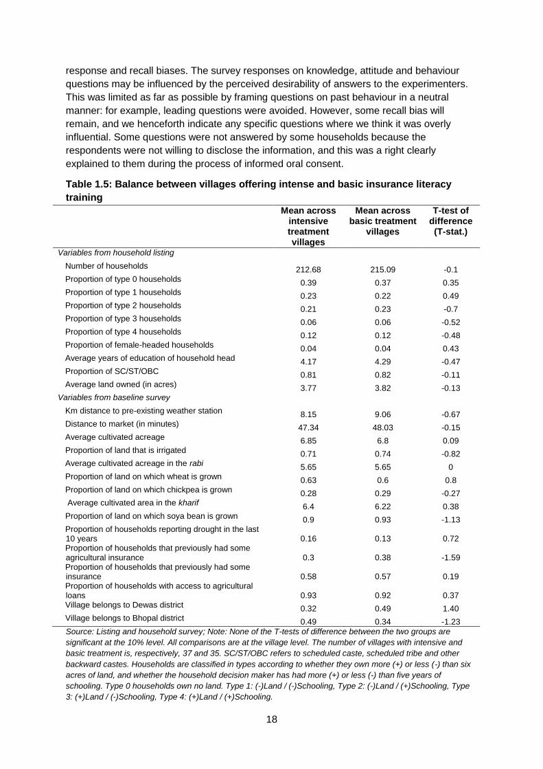
18

response and recall biases. The survey responses on knowledge, attitude and behaviour

questions may be influenced by the perceived desirability of answers to the experimenters.

This was limited as far as possible by framing questions on past behaviour in a neutral

manner: for example, leading questions were avoided. However, some recall bias will

remain, and we henceforth indicate any specific questions where we think it was overly

influential. Some questions were not answered by some households because the

respondents were not willing to disclose the information, and this was a right clearly

explained to them during the process of informed oral consent.

Table 1.5: Balance between villages offering intense and basic insurance literacy

training

Mean across intensive treatment villages

Mean across basic treatment

villages

T-test of difference (T-stat.)

Variables from household listing

Number of households 212.68 215.09 -0.1 Proportion of type 0 households 0.39 0.37 0.35 Proportion of type 1 households 0.23 0.22 0.49 Proportion of type 2 households 0.21 0.23 -0.7 Proportion of type 3 households 0.06 0.06 -0.52 Proportion of type 4 households 0.12 0.12 -0.48 Proportion of female-headed households 0.04 0.04 0.43 Average years of education of household head 4.17 4.29 -0.47 Proportion of SC/ST/OBC 0.81 0.82 -0.11 Average land owned (in acres) 3.77 3.82 -0.13

Variables from baseline survey Km distance to pre-existing weather station 8.15 9.06 -0.67 Distance to market (in minutes) 47.34 48.03 -0.15 Average cultivated acreage 6.85 6.8 0.09 Proportion of land that is irrigated 0.71 0.74 -0.82 Average cultivated acreage in the rabi 5.65 5.65 0 Proportion of land on which wheat is grown 0.63 0.6 0.8 Proportion of land on which chickpea is grown 0.28 0.29 -0.27 Average cultivated area in the kharif 6.4 6.22 0.38 Proportion of land on which soya bean is grown 0.9 0.93 -1.13 Proportion of households reporting drought in the last 10 years 0.16 0.13 0.72 Proportion of households that previously had some agricultural insurance 0.3 0.38 -1.59 Proportion of households that previously had some insurance 0.58 0.57 0.19 Proportion of households with access to agricultural loans 0.93 0.92 0.37 Village belongs to Dewas district 0.32 0.49 1.40 Village belongs to Bhopal district 0.49 0.34 -1.23

Source: Listing and household survey; Note: None of the T-tests of difference between the two groups are

significant at the 10% level. All comparisons are at the village level. The number of villages with intensive and

basic treatment is, respectively, 37 and 35. SC/ST/OBC refers to scheduled caste, scheduled tribe and other

backward castes. Households are classified in types according to whether they own more (+) or less (-) than six

acres of land, and whether the household decision maker has had more (+) or less (-) than five years of

schooling. Type 0 households own no land. Type 1: (-)Land / (-)Schooling, Type 2: (-)Land / (+)Schooling, Type

3: (+)Land / (-)Schooling, Type 4: (+)Land / (+)Schooling.

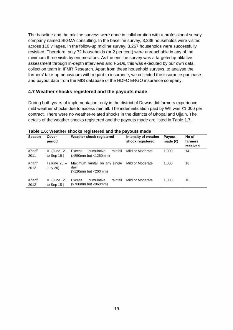
19

The baseline and the midline surveys were done in collaboration with a professional survey

company named SIGMA consulting. In the baseline survey, 3,339 households were visited

across 110 villages. In the follow-up midline survey, 3,267 households were successfully

revisited. Therefore, only 72 households (or 2 per cent) were unreachable in any of the

minimum three visits by enumerators. As the endline survey was a targeted qualitative

assessment through in-depth interviews and FGDs, this was executed by our own data

collection team in IFMR Research. Apart from these household surveys, to analyse the

farmers’ take-up behaviours with regard to insurance, we collected the insurance purchase

and payout data from the MIS database of the HDFC ERGO insurance company.

4.7 Weather shocks registered and the payouts made

During both years of implementation, only in the district of Dewas did farmers experience

mild weather shocks due to excess rainfall. The indemnification paid by WII was ₹1,000 per

contract. There were no weather-related shocks in the districts of Bhopal and Ujjain. The

details of the weather shocks registered and the payouts made are listed in Table 1.7.

Table 1.6: Weather shocks registered and the payouts made

Season Cover

period

Weather shock registered Intensity of weather

shock registered

Payout

made (₹)

No of

farmers

received

Kharif

2011

II (June 21

to Sep 15 )

Excess cumulative rainfall

(>850mm but <1250mm)

Mild or Moderate 1,000 14

Kharif

2012

I (June 25 –

July 20)

Maximum rainfall on any single day (>120mm but <200mm)

Mild or Moderate 1,000 18

Kharif

2012

II (June 21

to Sep 15 )

Excess cumulative rainfall (>700mm but <960mm)

Mild or Moderate 1,000 10

20

5. Methodology: Randomisation and evaluation design

5.1 Randomisation of insurance provision

Farmers who purchase insurance are a highly self-selected group. Current research in India

indicates that farmers more likely to buy insurance have higher levels of education and fewer

liquidity constraints (Cole et al. 2012). They may also differ in unobservable characteristics,

such as a tendency to buy new products. The behaviour of these farmers with respect to the

outcome variables of interest (identified in Evaluation Questions) is likely to be quite different

from those who do not purchase insurance. Simply comparing farmers with and without WII

will thus not tell us much about their impact, as preexisting underlying differences are likely

to confound the impact of receiving insurance. Farmers who were offered WII and chose not

to buy are thus not the appropriate counterfactual for those farmers who chose to buy.

To ensure the appropriate comparability between insured and uninsured farmers, we worked

with HDFC ERGO to randomly select villages to offer our product. As our product was not at

the stage of large-scale roll out, this approach was acceptable to the insurance company.

Randomising at the village level reduced the probability of contaminating the sample: if

randomisations were at the household level and a non-selected household wanted to

purchase insurance, it would have been difficult for HDFC ERGO marketing agents to

exclude them. Therefore, randomisation at the village level also mitigated the impact of

spillover effects on the estimates. Accordingly, a total of 110 villages were selected, and our

simplified WII products were offered in 72 of these villages selected at random, whilst

individuals in the remaining 38 villages formed the control group. More treatment villages

than control villages were selected, given the multiple treatment arms in this study. Villages

in Bhopal and Dewas were allocated to treatment and control categories using a random

draw with no stratification or blocking. Ujjain villages were allocated to treatment and control

categories separately, on account of the later inclusion of this district. As such, there was

stratification of the villages along district lines, and we include district dummies in all

regression analysis.

To ensure that the random selection of villages was successful, and thus treatment and

control villages did not differ statistically on the basis of observable characteristic existing

data sources (such as census data) were used to validate similarities on characteristics such

as distance to a nearby town, distance to the weather station, education, caste and

household-level socio-economic factors.

5.2 Randomisation of treatments

The 72 selected treatment villages were further categorised into different treatment

categories. The following two treatments were randomised at the village level:

Weather station: Thirty villages from Bhopal and Dewas were selected to be offered

insurance that has payments triggered by a weather station installed by the study

team. The remaining 29 villages (30 villages were originally chosen, but one was

dropped because its distance from the weather station was more than 20 km) from

these districts were offered insurance with payments triggered by pre-existing

weather stations in the corresponding district. This was done in order to exogenously

21

vary the degree of basis risk faced by households in the study villages. Only villages

in Dewas and Bhopal were eligible for this treatment, meaning that the 13 Ujjain

villages that received insurance used pre-existing reference stations.

Insurance literacy training: Thirty-seven villages were selected to receive intensive

insurance literacy training. The other 35 villages received the basic insurance literacy

training. This was done in order to exogenously vary the understanding of the

insurance product in the study villages.

There are thus four categories of treatment villages, as summarised in Table 2.1. The

number of villages in each category is given in brackets. Given the small number of villages

in each cell, interactions between the interventions will not be assessed.6

Table 2.1: Randomisation of treatment villages into four categories Existing weather station (E) and basic training (B) = 20 villages

Existing weather station (E) and intensive training (I) = 22 villages

E = 42

New weather station (N) and basic training (B) = 15 villages

New weather station (N) and intensive training (I) = 15 villages

N = 30

B = 35 I = 37

5.3 Selection of sample households

A listing exercise was conducted in all the selected villages (110 villages) before survey

work, training and insurance sales began. The listing exercise collected basic information on

each household’s characteristics. It collected information on age, gender and education of

the household head, caste, housing structure, landownership and main crop of production in

the rabi (winter) season.

The listing survey provided two important contributions to the study. Much of the

randomisation within this study was conducted at the village level, so aggregation of data

collected in the listing survey allowed us to calculate accurate village-level statistics in order

to ensure balanced treatments. Second, given that purchase rates of insurance tend to be

quite low, it was important for us to focus our energies on households that would be naturally

predisposed to purchase insurance. The information from the listing questionnaire allowed

us to identify these households and over-sample them.

Studies of insurance demand in India suggest that those who purchase weather index

insurance have larger landholdings and higher education levels than those who do not (Gine

et al. 2007). Data on education of the household decision maker and landholding of the

household that was collected in the listing survey was used to classify households into five

categories. Households in the first category, type 0 households, were those that did not own

any land. Weather insurance cannot be purchased by these households, so they were not

included in either the survey sample or in the training and marketing activities. Households

that owned land were further categorised into four types:

6 It was our initial intention to utilise the randomly allocated interventions described in this section as instruments

in IV approach to assess the consumption and production impacts of purchasing insurance. Since purchasers of

insurance are generally different in terms of a number of unobservable characteristics, this is one strategy to

obtain random variation in insurance purchase decisions. Given the very low take-up rates encountered,

however, we had to abandon this initial idea.

22

Type 1 households own less than or equal to 6 acres of land and have a

household decision maker with less than five years of schooling;

Type 2 households own less than or equal to 6 acres of land and have a

household decision maker with greater than or equal to five years of schooling;

Type 3 households own more than 6 acres of land and have a household

decision maker with less than five years of schooling; and

Type 4 households own more than 6 acres of land and have a household

decision maker with greater than or equal to five years of schooling.

On an average, the proportion of type 4 households is much lower than the proportion of

type 0, 1 or 2 households. However, it is type 4 households that are most likely to buy

insurance, so we oversampled these households for inclusion in our study.

In each village, 30 households were selected. We designed the sampling strategy such that

the proportion of type 4 households in the sample selected from each village would be 0.5.

Three type 1 households were randomly selected from all type 1 households, and six type 2

households, six type 3 households and 15 type 4 households. A summary is provided in

Table 2.2.

Table 2.2: Household types, based on education and landownership of household

decision makers

Less than 5 yrs of schooling

Greater than or equal to 5 yrs of schooling

Greater than 0 acres of land, less than or equal to 5 acres of land

Type 1 (3 included in activities)

Type 2 (6 included in activities)

Greater than 5 acres of land Type 3 (6 included in activities)

Type 4 (15 included in activities)

5.4 Evaluation design

A baseline survey was conducted before launching the weather insurance product in kharif

2011; this was followed by a midline survey for assessing the impact of the product, which

was conducted after the completion of the kharif 2011 cropping season. The baseline and

midline surveys were conducted for 30 households in each of the 38 control and 72

treatment villages. A comparison of differences in outcome variables between the baseline

and midline survey of control and treatment villages (difference in difference estimation)

provided us with a test of the impact of offering our simplified WII to the farmers.

On the other hand, the product take-up rate by the farmers during kharif 2011 was very low

(6 per cent of sample). Since only a low proportion of households in the sample purchased

our WII, the power of tests on the impact of our product was lower than what the initial power

calculations indicated. Similarly, the same trend of low take-up rate (4 per cent) of our

product prevailed during the subsequent cropping season of kharif 2012. Considering the

fact that the quantitative impact of the interventions addressed through the project’s midline

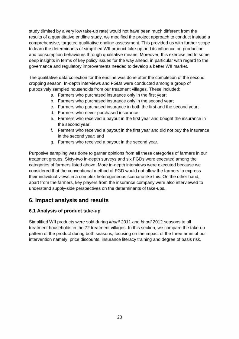
23

study (limited by a very low take-up rate) would not have been much different from the

results of a quantitative endline study, we modified the project approach to conduct instead a

comprehensive, targeted qualitative endline assessment. This provided us with further scope

to learn the determinants of simplified WII product take-up and its influence on production

and consumption behaviours through qualitative means. Moreover, this exercise led to some

deep insights in terms of key policy issues for the way ahead, in particular with regard to the

governance and regulatory improvements needed to develop a better WII market.

The qualitative data collection for the endline was done after the completion of the second

cropping season. In-depth interviews and FGDs were conducted among a group of

purposively sampled households from our treatment villages. These included:

a. Farmers who purchased insurance only in the first year;

b. Farmers who purchased insurance only in the second year;

c. Farmers who purchased insurance in both the first and the second year;

d. Farmers who never purchased insurance;

e. Farmers who received a payout in the first year and bought the insurance in

the second year;

f. Farmers who received a payout in the first year and did not buy the insurance

in the second year; and

g. Farmers who received a payout in the second year.

Purposive sampling was done to garner opinions from all these categories of farmers in our

treatment groups. Sixty-two in-depth surveys and six FGDs were executed among the

categories of farmers listed above. More in-depth interviews were executed because we

considered that the conventional method of FGD would not allow the farmers to express

their individual views in a complex heterogeneous scenario like this. On the other hand,

apart from the farmers, key players from the insurance company were also interviewed to

understand supply-side perspectives on the determinants of take-ups.

6. Impact analysis and results

6.1 Analysis of product take-up

Simplified WII products were sold during kharif 2011 and kharif 2012 seasons to all

treatment households in the 72 treatment villages. In this section, we compare the take-up

pattern of the product during both seasons, focusing on the impact of the three arms of our

intervention namely, price discounts, insurance literacy training and degree of basis risk.

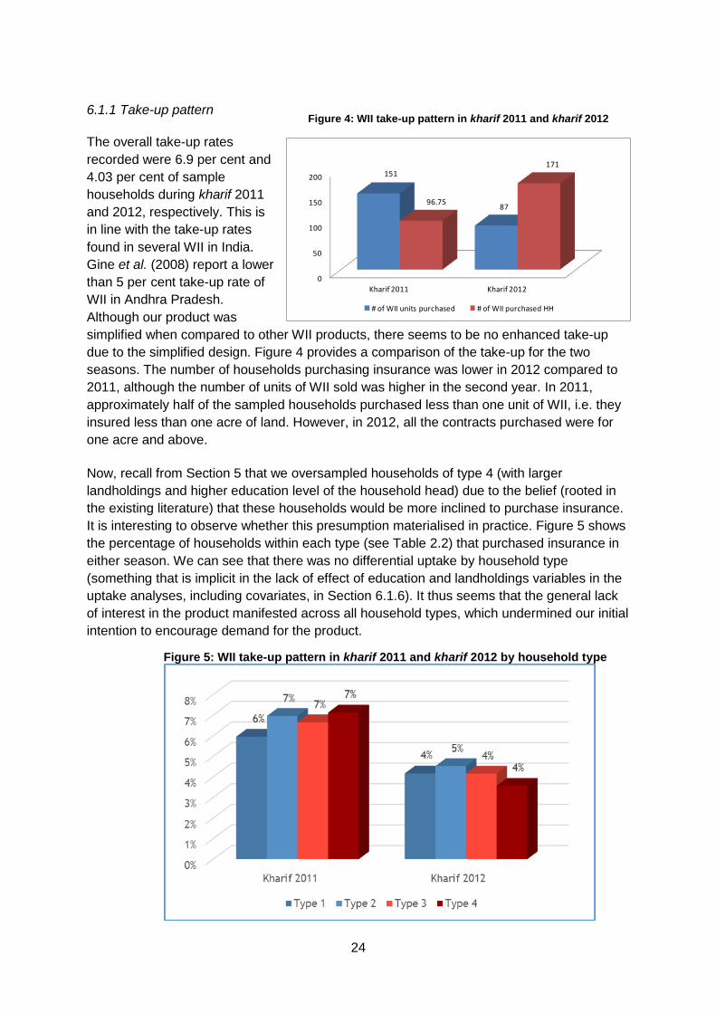
24

6.1.1 Take-up pattern

The overall take-up rates

recorded were 6.9 per cent and

4.03 per cent of sample

households during kharif 2011

and 2012, respectively. This is

in line with the take-up rates

found in several WII in India.

Gine et al. (2008) report a lower

than 5 per cent take-up rate of

WII in Andhra Pradesh.

Although our product was

simplified when compared to other WII products, there seems to be no enhanced take-up

due to the simplified design. Figure 4 provides a comparison of the take-up for the two

seasons. The number of households purchasing insurance was lower in 2012 compared to

2011, although the number of units of WII sold was higher in the second year. In 2011,

approximately half of the sampled households purchased less than one unit of WII, i.e. they

insured less than one acre of land. However, in 2012, all the contracts purchased were for

one acre and above.

Now, recall from Section 5 that we oversampled households of type 4 (with larger

landholdings and higher education level of the household head) due to the belief (rooted in

the existing literature) that these households would be more inclined to purchase insurance.

It is interesting to observe whether this presumption materialised in practice. Figure 5 shows

the percentage of households within each type (see Table 2.2) that purchased insurance in

either season. We can see that there was no differential uptake by household type

(something that is implicit in the lack of effect of education and landholdings variables in the

uptake analyses, including covariates, in Section 6.1.6). It thus seems that the general lack

of interest in the product manifested across all household types, which undermined our initial

intention to encourage demand for the product.

Figure 5: WII take-up pattern in kharif 2011 and kharif 2012 by household type

0

50

100

150

200

Kharif 2011 Kharif 2012

151

8796.75

171

# of WII units purchased # of WII purchased HH

Figure 4: WII take-up pattern in kharif 2011 and kharif 2012

25

6.1.2. Contract preference

As described in Section 4.1, there were two types of contracts offered for each peril

identified under every cover period. One security would pay on the occurrence of a very low

probability event representing severe yield losses, and the other security would pay on the

occurrence of a moderately probable event representing moderate and severe yield losses.

The objective behind this was to allow farmers to choose an insurance portfolio suited to

cover their specific combination of extreme and moderate risk. Naturally, the cost of the

contract for the low probability event was cheaper than the contract for the moderately

probable event. Interestingly, farmers’ preferences to insure against extreme or moderate

yield losses are quite different when we compare 2011 and 2012 data (Figure 6). During

kharif 2011, 87 per cent of farmers who purchased insurance bought the expensive contract

(i.e. they insured against moderate yield losses), whereas in kharif 2012, 94 per cent of

farmers who bought insurance preferred the cheaper contracts (i.e. they insured against

extreme yield losses). Moreover, a large proportion of the farmers who bought insurance

during kharif 2011 did not repurchase insurance in kharif 2012, except for a handful of 11

farmers.

6.1.3 Premium discounts

As elaborated in Section 4.3, four levels of discounts were given to the treatment households

which were approximately close to 15 per cent, 30 per cent, 45 per cent and 60 per cent of

the premium amount of the product offered to them during kharif 2011 and kharif 2012

cropping seasons.

0

20

40

60

80

100

120

140

160

Cheaper contracts (Extreme yield losses)

Expensive contracts (Moderate yield losses)

160

11

81

6

# of WII units purchased # of WII purchased HH

0

20

40

60

80

100

120

140

Cheaper contracts (Extreme yield losses)

Expensive contracts (Moderate yield losses)

13

83.75

14

137

# of WII units purchased # of WII purchased HH

kharif 2012

kharif 2011

Figure 6: Farmers preference for cheaper vs expensive WII contracts

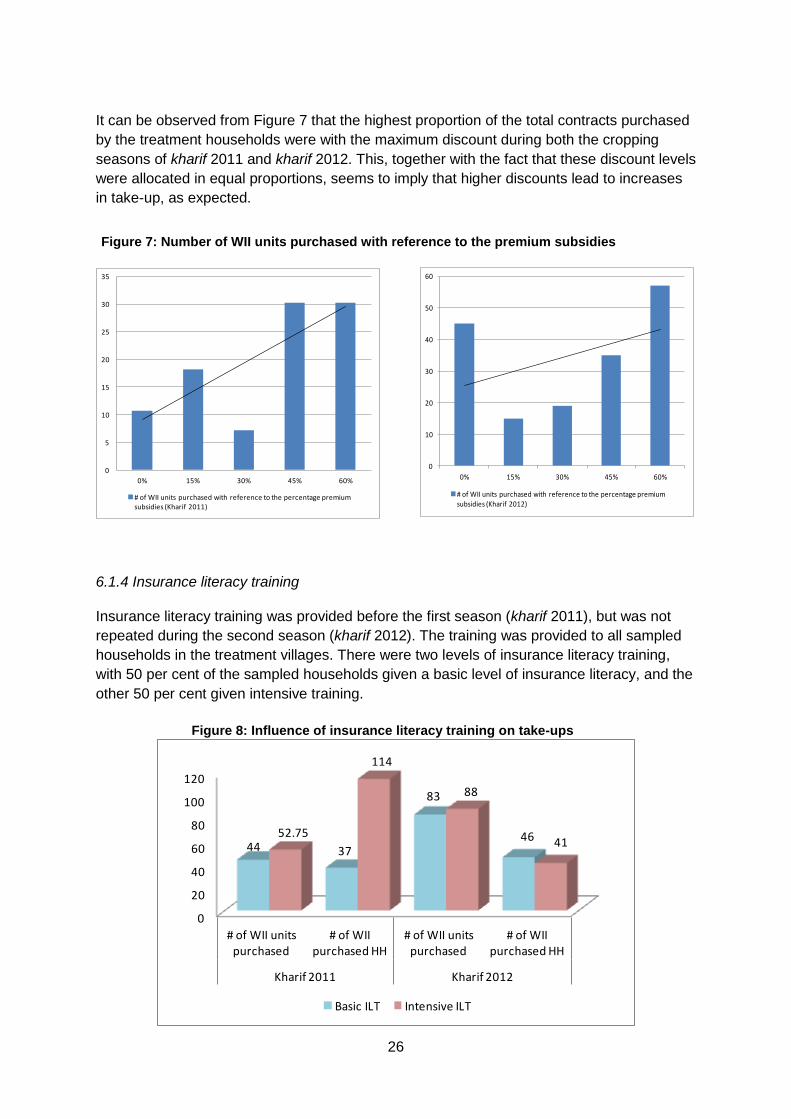
26

0

5

10

15

20

25

30

35

0% 15% 30% 45% 60%

# of WII units purchased with reference to the percentage premium subsidies (Kharif 2011)

0

10

20

30

40

50

60

0% 15% 30% 45% 60%

# of WII units purchased with reference to the percentage premium subsidies (Kharif 2012)

It can be observed from Figure 7 that the highest proportion of the total contracts purchased

by the treatment households were with the maximum discount during both the cropping

seasons of kharif 2011 and kharif 2012. This, together with the fact that these discount levels

were allocated in equal proportions, seems to imply that higher discounts lead to increases

in take-up, as expected.

6.1.4 Insurance literacy training

Insurance literacy training was provided before the first season (kharif 2011), but was not

repeated during the second season (kharif 2012). The training was provided to all sampled

households in the treatment villages. There were two levels of insurance literacy training,

with 50 per cent of the sampled households given a basic level of insurance literacy, and the

other 50 per cent given intensive training.

0

20

40

60

80

100

120

# of WII units purchased

# of WII purchased HH

# of WII units purchased

# of WII purchased HH

Kharif 2011 Kharif 2012

44 37

83

4652.75

114

88

41

Basic ILT Intensive ILT

Figure 7: Number of WII units purchased with reference to the premium subsidies

Figure 8: Influence of insurance literacy training on take-ups

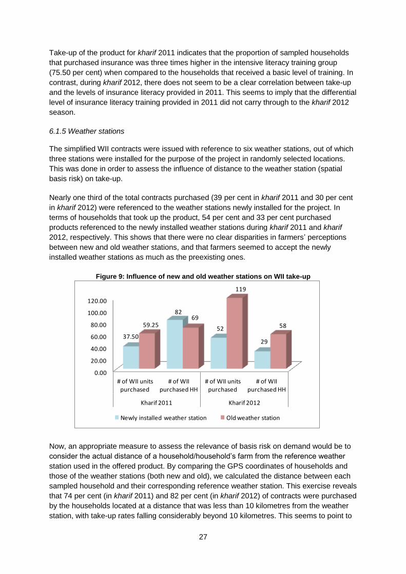
27

Take-up of the product for kharif 2011 indicates that the proportion of sampled households

that purchased insurance was three times higher in the intensive literacy training group

(75.50 per cent) when compared to the households that received a basic level of training. In

contrast, during kharif 2012, there does not seem to be a clear correlation between take-up

and the levels of insurance literacy provided in 2011. This seems to imply that the differential

level of insurance literacy training provided in 2011 did not carry through to the kharif 2012

season.

6.1.5 Weather stations

The simplified WII contracts were issued with reference to six weather stations, out of which

three stations were installed for the purpose of the project in randomly selected locations.

This was done in order to assess the influence of distance to the weather station (spatial

basis risk) on take-up.

Nearly one third of the total contracts purchased (39 per cent in kharif 2011 and 30 per cent

in kharif 2012) were referenced to the weather stations newly installed for the project. In

terms of households that took up the product, 54 per cent and 33 per cent purchased

products referenced to the newly installed weather stations during kharif 2011 and kharif

2012, respectively. This shows that there were no clear disparities in farmers’ perceptions

between new and old weather stations, and that farmers seemed to accept the newly

installed weather stations as much as the preexisting ones.

Figure 9: Influence of new and old weather stations on WII take-up

Now, an appropriate measure to assess the relevance of basis risk on demand would be to

consider the actual distance of a household/household’s farm from the reference weather

station used in the offered product. By comparing the GPS coordinates of households and

those of the weather stations (both new and old), we calculated the distance between each

sampled household and their corresponding reference weather station. This exercise reveals

that 74 per cent (in kharif 2011) and 82 per cent (in kharif 2012) of contracts were purchased

by the households located at a distance that was less than 10 kilometres from the weather

station, with take-up rates falling considerably beyond 10 kilometres. This seems to point to

0.00

20.00

40.00

60.00

80.00

100.00

120.00

# of WII units purchased

# of WII purchased HH

# of WII units purchased

# of WII purchased HH

Kharif 2011 Kharif 2012

37.50

82

52

29

59.2569

119

58

Newly installed weather station Old weather station

28

a significant impact of spatial basis risk on index insurance take-up. The next section

formalises this analysis by introducing distance to the reference weather station into an

econometric model of the household’s decision to purchase insurance.

6.1.6 Further analysis on the impact of interventions on take-up

We carried out an in-depth econometric analysis of take-up and found that the results are in

line with our descriptive analysis of take-up data. In this section, we begin with the analysis

of the kharif 2011 insurance purchasing season. In particular, we test the village-level

interventions formally by estimating the intent to treat effect (ITT) as follows:

dij = α + βt tj + εij (6.1)

Where dij is a measure of insurance demand for individual i in village j and tj indicates the

treatment that the village received. We test the impact of price discounts formally by

estimating the ITT as follows:

dij = α + βppij + εij (6.2)

54

60

37

0

3530

17

5

0

10

20

30

40

50

60

70

< 5 Km 5-10 Km 10-15 Km 15-20 Km

# of WII purchased HH Kharif 2011 # of WII purchased HH Kharif 2012

38.7532.5

25.5

0

58

83

21

9

0

10

20

30

40

50

60

70

80

90

< 5 Km 5-10 Km 10-15 Km 15-20 Km

# of WII units purchased Kharif 2011 # of WII units purchased Kharif 2012

Figure 10: WII take-up with reference to the distance from weather station

29

Where pij indicates the price discount that individual i in village j received. Given the

orthogonality of each treatment to the other treatments, we can estimate the impact of each

treatment on demand separately. When we consider the impact of basis risk on demand, we

also use the following estimation strategy. We instrument distance to weather station using

allocation to a new weather station as an instrument. Specifically, the estimation strategy

used is:

dij = α + βdistdistij + εij (6.3)

Where distij is the estimate derived from the following equation (where tj in this case refers

to whether or not insurance was triggered by a newly placed weather station):

distij = α + βttj + εij . (6.4)

In Tables 6.1 and 6.2, we present results on the impact of our three interventions—price

discounts, weather station investments and training—on insurance demand.7 Table 3.1

presents results using a dependent variable that takes the value of 1 when a household

purchased insurance. In Table 3.2, the dependent variable is the log of the amount of land

insured. Columns 1 to 4 look at each of the interventions separately, whilst in the last two

columns, we simultaneously estimate the impact on all of the interventions. Given that each

intervention was randomly allocated and we tested that the weather station and intensive

training intervention were orthogonally allocated, we should not observe any difference from

considering the impact of all treatments at the same time.

First, we note that the proportion of households purchasing insurance is significantly higher

among sample households in Bhopal than in Dewas or Ujjain. This may be possibly related

to the higher level of marketing effort and organisation in Bhopal than in the other districts.

As discussed earlier, marketing in Dewas suffered some setbacks for the late season

policies. Ujjain was a new district for HDFC, and insurance literacy training and marketing

followed each other closely in this district, perhaps leaving farmers little time to decide

whether or not they would buy insurance.

Second, we look at the impact of being offered a price discount. Discounts varied from ₹0 to

₹180 in Bhopal and Dewas, and ₹0 to ₹120 in Ujjain. The independent variable on discounts

in Table 3.1 is the ratio of the discount value to price of the cheapest policy. The price of this

policy is ₹265 in Bhopal and Dewas and ₹165 in Ujjain. Since the ratio of the price of

expensive to inexpensive policy is constant across all districts, this ratio is a good measure

7 In all of the subsequent analyses, standard errors are clustered at the village level, since this is the main level at

which we conduct the random assignment of our treatments. Nevertheless, best practice indicates that, when

using the random assignment of weather stations in our analysis, standard errors should be clustered at this

level. The first problem with doing so is that we have an extremely low number of clusters (six weather stations in

total), which is far from enough for achieving any asymptotic properties of the estimator for the standard errors.

Second, this type of concern arises from the possibility of common error components across study units within a

given cluster. This is of course reasonable when the cluster is a village, a district, or other economic aggregate

sharing common social and economic factors. In our case, however, the aggregate unit is only created artificially

by taking into consideration an arbitrary threshold of geographic proximity to randomly-placed weather stations.

Given this, we expect these common components in the error term to be of much lower importance than in other

cases of randomised assignment. This said, we did run the analyses clustering at the weather station level and

find, as expected, that standard errors increase substantially, rendering all coefficients in the tables statistically

insignificant.

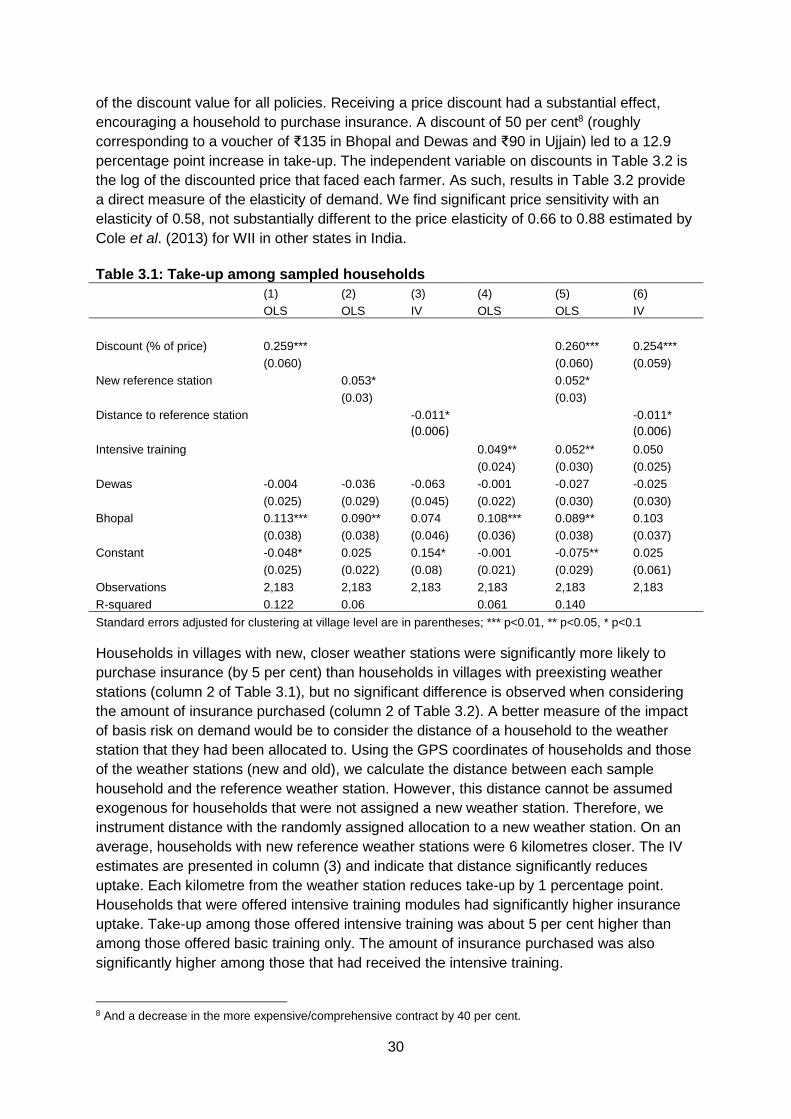
30

of the discount value for all policies. Receiving a price discount had a substantial effect,

encouraging a household to purchase insurance. A discount of 50 per cent8 (roughly

corresponding to a voucher of ₹135 in Bhopal and Dewas and ₹90 in Ujjain) led to a 12.9

percentage point increase in take-up. The independent variable on discounts in Table 3.2 is

the log of the discounted price that faced each farmer. As such, results in Table 3.2 provide

a direct measure of the elasticity of demand. We find significant price sensitivity with an

elasticity of 0.58, not substantially different to the price elasticity of 0.66 to 0.88 estimated by

Cole et al. (2013) for WII in other states in India.

Table 3.1: Take-up among sampled households

(1) (2) (3) (4) (5) (6)

OLS OLS IV OLS OLS IV

Discount (% of price) 0.259*** 0.260*** 0.254***

(0.060) (0.060) (0.059)

New reference station 0.053* 0.052*

(0.03) (0.03)

Distance to reference station -0.011* -0.011*

(0.006) (0.006)

Intensive training 0.049** 0.052** 0.050

(0.024) (0.030) (0.025)

Dewas -0.004 -0.036 -0.063 -0.001 -0.027 -0.025

(0.025) (0.029) (0.045) (0.022) (0.030) (0.030)

Bhopal 0.113*** 0.090** 0.074 0.108*** 0.089** 0.103

(0.038) (0.038) (0.046) (0.036) (0.038) (0.037)

Constant -0.048* 0.025 0.154* -0.001 -0.075** 0.025

(0.025) (0.022) (0.08) (0.021) (0.029) (0.061)

Observations 2,183 2,183 2,183 2,183 2,183 2,183

R-squared 0.122 0.06 0.061 0.140

Standard errors adjusted for clustering at village level are in parentheses; *** p<0.01, ** p<0.05, * p<0.1

Households in villages with new, closer weather stations were significantly more likely to

purchase insurance (by 5 per cent) than households in villages with preexisting weather

stations (column 2 of Table 3.1), but no significant difference is observed when considering

the amount of insurance purchased (column 2 of Table 3.2). A better measure of the impact

of basis risk on demand would be to consider the distance of a household to the weather

station that they had been allocated to. Using the GPS coordinates of households and those

of the weather stations (new and old), we calculate the distance between each sample

household and the reference weather station. However, this distance cannot be assumed

exogenous for households that were not assigned a new weather station. Therefore, we

instrument distance with the randomly assigned allocation to a new weather station. On an

average, households with new reference weather stations were 6 kilometres closer. The IV

estimates are presented in column (3) and indicate that distance significantly reduces

uptake. Each kilometre from the weather station reduces take-up by 1 percentage point.

Households that were offered intensive training modules had significantly higher insurance

uptake. Take-up among those offered intensive training was about 5 per cent higher than

among those offered basic training only. The amount of insurance purchased was also

significantly higher among those that had received the intensive training.

8 And a decrease in the more expensive/comprehensive contract by 40 per cent.

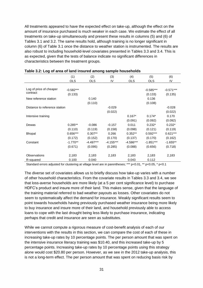
31

All treatments appeared to have the expected effect on take-up, although the effect on the

amount of insurance purchased is much weaker in each case. We estimate the effect of all

treatments on take-up simultaneously and present these results in columns (5) and (6) of

Tables 3.1 and 3.2. The same results hold, although training is no longer significant in

column (6) of Table 3.1 once the distance to weather station is instrumented. The results are

also robust to including household-level covariates presented in Tables 3.3 and 3.4. This is

as expected, given that the tests of balance indicate no significant differences in

characteristics between the treatment groups.

Table 3.2: Log of area of land insured among sample households

(1) (2) (3) (4) (5) (6)

OLS OLS IV OLS OLS IV

Log of price of cheaper contract

-0.582*** -0.585*** -0.571***

(0.133) (0.133) (0.135)

New reference station 0.140 0.136

(0.110) (0.108)

Distance to reference station -0.029 -0.028

(0.022) (0.022)

Intensive training 0.167* 0.174* 0.170

(0.091) (0.092) (0.092)

Dewas 0.285** -0.086 -0.157 0.011 0.232* 0.232*

(0.110) (0.119) (0.158) (0.098) (0.121) (0.119)

Bhopal 0.656*** 0.307** 0.266 0.352** 0.592*** 0.621***

(0.172) (0.152) (0.170) (0.137) (0.170) (0.162)

Constant -1.770** -4.497*** -4.155*** -4.586*** -1.851*** -1.655**

(0.671) (0.095) (0.285) (0.088) (0.656) (0.718)

Observations 2,183 2,183 2,183 2,183 2,183 2,183

R-squared 0.100 0.040 0.043 0.112

Standard errors adjusted for clustering at village level are in parentheses; *** p<0.01, ** p<0.05, * p<0.1

The diverse set of covariates allows us to briefly discuss how take-up varies with a number

of other household characteristics. From the covariate results in Tables 3.3 and 3.4, we see

that loss-averse households are more likely (at a 5 per cent significance level) to purchase

HDFC’s product and insure more of their land. This makes sense, given that the language of

the training material referred to bad weather payouts as losses. Other covariates do not

seem to systematically affect the demand for insurance. Weakly significant results seem to

point towards households having previously purchased weather insurance being more likely

to buy insurance and insure more of their land, and household previously able to access

loans to cope with the last drought being less likely to purchase insurance, indicating

perhaps that credit and insurance are seen as substitutes.

While we cannot compute a rigorous measure of cost-benefit analysis of each of our

interventions with the results in this section, we can compare the cost of each of these in

increasing take-up rates by 10 percentage points. The per person amount that was spent on

the intensive insurance literacy training was $10.40, and this increased take-up by 5

percentage points. Increasing take-up rates by 10 percentage points using this strategy

alone would cost $20.80 per person. However, as we see in the 2012 take-up analysis, this

is not a long-term effect. The per person amount that was spent on reducing basis risk by

32

installing new trigger weather stations was $6.67. This also increased take-up by 5

percentage points. Increasing take-up rates by 10 percentage points using this strategy

alone would cost $13.34 per person. This is more cost-effective than insurance literacy

training. The results in Table 3.1 suggest that to increase take-up rates by 10 percentage

points, a discount of ₹115 or about $2.30 per policy is needed. In Bhopal and Dewas, we

also spent $2.97 distributing vouchers to each farmer, but this is because we were

randomising the price within a village. In Ujjain, the cost of administering the discount was

non-existent as it was just a matter of the HDFC agent telling farmers. Either way, this

strategy for increasing purchases of insurance is the most cost-effective of the three.

33

Table 3.3: Sample households, take-up (adding covariates) (1) (2) (3) (4) (5) (6) OLS OLS IV OLS OLS IV

Ratio of discount to price 0.264*** 0.267*** 0.261***

(0.061) (0.061) (0.061) New reference station 0.050* 0.051*

(0.030) (0.029) Distance to reference station -0.007** -0.010*

(0.004) (0.006) Intensive training 0.052** 0.056** 0.050**

(0.024) (0.024) (0.024) Dewas -0.007 -0.036 -0.039 -0.002 -0.033 -0.037

(0.028) (0.033) (0.033) (0.026) (0.033) (0.034) Bhopal 0.111*** 0.089** 0.098*** 0.103*** 0.086** 0.096**

(0.040) (0.038) (0.035) (0.033) (0.038) (0.037) Years of schooling 0.002 0.002 0.001 0.002 0.002 0.001

(0.002) (0.002) (0.002) (0.002) (0.002) (0.002) Head is a male -0.004 -0.002 0.013 0.001 0.007 0.021

(0.030) (0.029) (0.029) (0.030) (0.029) (0.030) Household is SC, ST or OBC 0.017 0.026* 0.023 0.024* 0.013 0.011

(0.014) (0.015) (0.016) (0.014) (0.014) (0.015) Head holds official village position

-0.004 0.009 0.012 0.013 0.003 0.006

(0.027) (0.029) (0.029) (0.028) (0.027) (0.027) Member of cooperative -0.010 -0.008 -0.008 -0.007 -0.016 -0.016

(0.016) (0.016) (0.016) (0.017) (0.015) (0.015) Acres of land owned 0.002 0.002 0.002* 0.002 0.002 0.002*

(0.001) (0.001) (0.001) (0.001) (0.001) (0.001) Log of total assets -0.001 -0.003 -0.004 -0.001 -0.000 -0.002

(0.005) (0.006) (0.005) (0.006) (0.005) (0.005) Owns a bank account -0.007 -0.010 -0.013 -0.012 -0.007 -0.010

(0.013) (0.014) (0.014) (0.014) (0.012) (0.012) Can obtain ₹20,000 for emergency

0.004 0.005 0.002 0.005 0.009 0.006

(0.015) (0.014) (0.014) (0.015) (0.014) (0.014) Bought insurance before 0.016 0.009 0.010 0.011 0.017 0.017

(0.016) (0.017) (0.016) (0.016) (0.016) (0.015) Trust in private insurance -0.004 -0.001 -0.005 -0.006 0.000 -0.003

(0.012) (0.013) (0.013) (0.012) (0.013) (0.013) Expected government aid for crops

-0.007 -0.005 -0.002 -0.007 -0.013 -0.009

(0.011) (0.011) (0.011) (0.011) (0.011) (0.011) Took out loan for last drought -0.022 -0.019 -0.023 -0.024* -0.024 -0.028*

(0.015) (0.015) (0.015) (0.015) (0.015) (0.015) Insurance knowledge score(/5) 0.004 0.002 0.003 0.003 0.000 0.001

(0.006) (0.006) (0.005) (0.006) (0.005) (0.005) RA game, chose option 2 0.017 0.015 0.008 0.017 0.024 0.016

(0.018) (0.018) (0.022) (0.018) (0.017) (0.021) RA game, chose option 3 0.013 0.003 -0.006 0.005 0.018 0.009

(0.022) (0.022) (0.024) (0.022) (0.021) (0.023) RA game, chose option 4 0.004 -0.002 -0.010 -0.001 0.011 0.003

(0.018) (0.017) (0.021) (0.018) (0.016) (0.020) RA game, chose option 5 -0.004 -0.005 -0.011 -0.006 -0.003 -0.009

(0.021) (0.021) (0.024) (0.022) (0.020) (0.023) Ambiguity averse 0.013 0.014 0.006 0.015 0.014 0.006

(0.014) (0.015) (0.018) (0.014) (0.014) (0.018) Loss averse 0.024** 0.023** 0.033*** 0.022** 0.023** 0.033***

(0.010) (0.011) (0.013) (0.011) (0.010) (0.012) Constant -0.083 0.007 0.132 -0.047 -0.127 0.006

(0.088) (0.103) (0.123) (0.100) (0.090) (0.114)

Observations 2,164 2,164 2,164 2,164 2,164 2,164 R-squared 0.134 0.070 0.005 0.072 0.153 0.082

Standard errors adjusted for clustering at village level are in parentheses. Risk aversion (RA) choices are from a hypothetical Binswanger lottery survey question, where choice 1 is the least risk averse option. *** p<0.01, ** p<0.05, * p<0.1

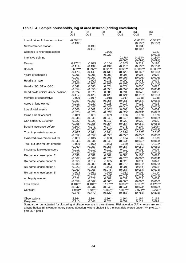
34

Table 3.4: Sample households, log of area insured (adding covariates) (1) (2) (3) (4) (5) (6) OLS OLS IV OLS OLS IV Log of price of cheaper contract -0.594*** -0.602*** -0.589*** (0.137) (0.138) (0.138) New reference station 0.130 0.134 (0.110) (0.108) Distance to reference station -0.026 -0.027 (0.022) (0.022) Intensive training 0.178* 0.194** 0.180** (0.090) (0.091) (0.091) Dewas 0.270** -0.095 -0.104 -0.003 0.211 0.198 (0.119) (0.139) (0.134) (0.113) (0.135) (0.131) Bhopal 0.652*** 0.297** 0.320** 0.328** 0.586*** 0.608*** (0.173) (0.149) (0.136) (0.129) (0.168) (0.160) Years of schooling 0.006 0.005 0.003 0.005 0.004 0.002 (0.007) (0.007) (0.007) (0.007) (0.006) (0.006) Head is a male 0.007 -0.004 0.033 0.009 0.043 0.079 (0.106) (0.103) (0.103) (0.107) (0.104) (0.106) Head is SC, ST or OBC 0.042 0.080 0.074 0.074 0.030 0.025 (0.054) (0.056) (0.058) (0.052) (0.052) (0.054) Head holds official village position 0.024 0.075 0.083 0.091 0.048 0.055 (0.117) (0.123) (0.123) (0.121) (0.115) (0.115) Member of cooperative -0.029 -0.017 -0.018 -0.017 -0.048 -0.048 (0.057) (0.057) (0.055) (0.061) (0.054) (0.052) Acres of land owned 0.011 0.020 0.023 0.017 0.012 0.015 (0.041) (0.041) (0.041) (0.040) (0.039) (0.039) Log of total assets 0.006 0.002 -0.002 0.008 0.009 0.004 (0.025) (0.026) (0.024) (0.027) (0.024) (0.023) Owns a bank account -0.019 -0.031 -0.039 -0.036 -0.020 -0.028 (0.046) (0.049) (0.049) (0.048) (0.042) (0.042) Can obtain ₹20,000 for emergency

0.022 0.025 0.017 0.029 0.039 0.030 (0.055) (0.055) (0.054) (0.054) (0.052) (0.051) Bought insurance before 0.100 0.071 0.074 0.078 0.104 0.106* (0.064) (0.067) (0.065) (0.065) (0.065) (0.063) Trust in private insurance -0.017 -0.011 -0.021 -0.024 -0.007 -0.017 (0.052) (0.057) (0.053) (0.053) (0.056) (0.053) Expected government aid for crops

-0.031 -0.015 -0.008 -0.024 -0.048 -0.039 (0.043) (0.044) (0.043) (0.044) (0.042) (0.041) Took out loan for last drought -0.080 -0.072 -0.083 -0.089 -0.091 -0.102* (0.060) (0.057) (0.058) (0.057) (0.059) (0.059) Insurance knowledge score 0.011 0.010 0.012 0.010 0.001 0.004 (0.021) (0.022) (0.022) (0.023) (0.022) (0.021) RA game, chose option 2 0.086 0.081 0.062 0.088 0.108 0.088 (0.067) (0.069) (0.076) (0.070) (0.066) (0.074) RA game, chose option 3 0.055 0.017 -0.005 0.026 0.071 0.047 (0.080) (0.080) (0.082) (0.079) (0.077) (0.079) RA game, chose option 4 0.023 -0.003 -0.023 0.001 0.044 0.023 (0.069) (0.066) (0.075) (0.068) (0.064) (0.073) RA game, chose option 5 -0.003 -0.011 -0.026 -0.013 0.001 -0.014 (0.076) (0.077) (0.083) (0.078) (0.073) (0.079) Ambiguity averse 0.021 0.027 0.007 0.031 0.023 0.002 (0.059) (0.062) (0.066) (0.060) (0.060) (0.066) Loss averse 0.104** 0.101** 0.127*** 0.097** 0.100** 0.126*** (0.042) (0.044) (0.045) (0.044) (0.041) (0.042) Constant -1.968** -4.706*** -4.389*** -4.887*** -2.074*** -1.766** (0.778) (0.470) (0.522) (0.453) (0.753) (0.815) Observations 2,164 2,164 2,164 2,164 2,164 2,164 R-squared 0.110 0.048 0.023 0.052 0.123 0.094 Standard errors adjusted for clustering at village level are in parentheses. Risk aversion (RA) choices are from a hypothetical Binswanger lottery survey question, where choice 1 is the least risk averse option. *** p<0.01, ** p<0.05, * p<0.1

35

6.2 Midline impact analysis

The midline survey provides us with an array of data on which we can test the impact of the

kharif 2011 intervention. First, we can measure the impact of offering insurance—ITT

effect—on a set of household characteristics. Second, since we have information on which

households actually bought insurance products, we are also interested in measuring the

effect of actual insurance purchase on their farming outcomes and decisions. While

answering these two questions may require different econometric strategies, we begin by

using ANCOVA to analyse both sets of questions.

Given that we have data on household characteristics for two time periods, baseline and

midline, we can either use ANCOVA, estimate differences between treatment and control in

the period post intervention, or implement a difference-in-differences estimator. If there is

correlation between the midline and baseline household characteristics, the ANCOVA

estimator is strictly more efficient and hence more statistically powerful than the post-

intervention estimator alone. Furthermore, the ANCOVA estimator is weakly more efficient

and hence more statistically powerful than the difference-in-differences for all levels of

autocorrelation in the variable of interest (McKenzie 2011). Due to this statistical superiority,

we prefer the ANCOVA approach for both: an estimate of ITT of offering insurance and the

impact of purchasing insurance. The general regression specification is presented in (6.5)

and the estimator of interest is approximated in (6.6), where Y is one variable of interest (e.g.

income from soya bean production) that takes values across two different time periods 0 and

1, and TREATi,1 takes a value of 1 if household i received a specific treatment, e.g. intensive

training, and 0 if it did not.

𝑌𝑖,1 = 𝛼 + 𝛾𝑇𝑅𝐸𝐴𝑇𝑖,1 + 𝜃𝑌𝑖,0 + 𝜀𝑖,1 (6.5)

𝛾 = (𝑌1

𝑇 − 𝑌1𝐶) − 𝜃(𝑌0

𝑇 − 𝑌0𝐶)

(6.6)

Equations (6.5) and (6.6) also present, respectively, the specification and the estimator of

the ITT effect of being offered insurance, where TREATi,1 takes a value of 1 if insurance was

offered to household I, and 0 otherwise.

For the set of variables we are interested in, we have calculated the minimum detectable

effect (MDE) of a test on the statistical significance of the coefficient gamma in equation

(6.5). Here, the minimum detectable effect is defined as the true ITT, which gives us a

statistical power of at least 0.8 in a two-sided test of the null hypothesis that the ITT is equal

to zero9. We would like to have a minimum detectable effect that is as small as possible in

order to detect true population effects (through the estimated gamma) in our random sample.

Table 3.5 shows the MDE of our ITT regressions. The first column presents the average of

the variable in the control group. The second column shows the minimum difference from the

control mean that would be possible to detect by a test on gamma with a power of more than

or equal to 0.8 (and thus a probability of type II error less than or equal to 0.2). For example,

9 In order to calculate the MDE, we estimate sample means and standard deviations (adjusted by the intra-cluster

correlation of the errors at the village level) for both control and treatment group, and an overall autocorrelation

coefficient between baseline and follow-up. These, together with the total sample sizes of both groups, are then

used as inputs into the sampsi command in STATA, which uses a variance for the estimated gamma coefficient

like the one discussed in McKenzie (2011).

36

if the population’s true (ITT) effect of insurance on the log of total acres sowed with soya

bean were less than 0.11, a statistical test of the significance of the gamma coefficient in

equation (6.5) would incorrectly fail to reject the null (thus claiming no effect when in fact it

exists) in more than 20 per cent of the draws of a random sample from the population

(keeping constant the probability of type I error at 5 per cent). In other words, and with our

current sample size, in order to keep the type II error probability below 20 per cent (power

above 80 per cent) and thus identify an effect when this truly exists, the true (population)

average impact of providing insurance on the log of total acres sowed with soya bean would

need to be larger than 0.11 acres per farmer.

Equations (6.7) and (6.8) below present the second and first stage of the main ATE (average

treatment effect) regression in our subsequent analysis. In order to calculate the average

treatment effect of purchasing insurance, we instrument insurance purchase with the

exogenous variations in our study: assignment of weather station, price discount vouchers

and intensive training:

𝑌𝑖,1 = 𝛼 + 𝛾𝑃𝑈𝑅𝐶𝐻𝐴𝑆𝐸𝑖,1 + 𝜃𝑌𝑖,0 + 𝜀𝑖,1 (6.7)

𝑃𝑈𝑅𝐶𝐻𝐴𝑆𝐸𝑖,1 = 𝛽 + 𝛽1𝑇𝑅𝐴𝐼𝑁𝐼𝑁𝐺𝑖,1 + 𝛽2𝑆𝑇𝐴𝑇𝐼𝑂𝑁𝑖,1𝛾 + 𝛽3𝑉𝑂𝑈𝐶𝐻𝐸𝑅𝑖,1 + 𝛽4𝑌𝑖,0 + 𝜇𝑖,1 (6.8)

We present estimates of the MDE of gamma in regression (6.7) in Table 3.6. In this case,

the MDE constitutes an MDE calculation for an un-instrumented endogenous variable.

Therefore, the approximations in Table 3.6 should be taken with caution. When we compare

Tables 3.5 and 3.6, we see that the intervals are generally much higher for Table 3.6, those

applicable to the ATE regressions. The first reason is that the sample is restricted and only

includes households that were offered insurance—otherwise the interpretation of the gamma

coefficient is not the intended ATE of insurance purchase over not purchasing insurance

when insurance is offered. The smaller sample size thus increases the standard deviations

used in our MDE calculations. Furthermore, only 151 households purchased insurance.

Therefore, the standard error for the treatment group, i.e. those who were offered insurance,

is much larger and thus contributes to a higher MDE. Finally, while in our ITT analysis we

have a relatively balanced ratio of treatment to control observations (1.92 with a total of

3,228 observations), the ratio of treatment to control observations in our analysis of the

uptake of insurance is only 0.08, with a total of 2,123 observations. In conclusion, the larger

MDE for our ATE estimations implies that we would need to face a much higher population

effect (in comparison to the ITT estimations) in order to be able to achieve the same amount

of power. In other words, these MDE calculations imply that it will be very hard for us to find

statistically significant effects from holding insurance on different production variables unless

the true effect of insurance were implausibly large.

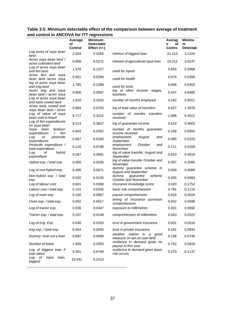
37

Table 3.5: Minimum detectable effect of the comparison between average of treatment

and control in ANCOVA for ITT regressions

Average of Control

Minimum Detectable Effect (+/-)

Average of Control

Minimum Detectable Effect (+/-)

Log acres of soya bean land

2.004 0.1093 interest of biggest loan 21.113 3.1324

Acres soya bean land / acres cultivated land

0.956 0.0271 interest of agricultural input loan 19.012 3.5537

Log of acres soya bean and fert land

1.978 0.1227 used for inputs

0.656 0.0968

Acres fert and soya bean land /acres soya bean land

0.961 0.0294 used for health

0.074 0.0356

log of acres soya bean and irrig land

1.785 0.1399 used for tools

0.066 0.0403

Acres irrig and soya bean land / acres soya bean land

0.806 0.0597 log of other income: wages, business

5.047 0.8485

Log of acres soya bean and early sowed land

1.810 0.1915 number of months employed 4.262 0.9011

Acres early sowed and soya bean land / acres soya bean land

0.883 0.0703 log of total value of transfers 6.627 1.3978

Log of value of soya bean sold in kharif

9.717 0.3212 number of months transfers received

1.998 0.4512

Log of fert expenditures on soya bean

8.214 0.3827 log of guarantee income 0.519 0.4663

Soya bean fertiliser expenditures / fert expenditures

0.943 0.0352 number of months guarantee income received

0.108 0.0993

Log of pesticide expenditures

0.667 0.0160 employment August and September

0.085 0.0223

Pesticide expenditure / total expenditure

0.120 0.0198 employment October and November

0.111 0.0269

Log of hybrid expenditure

0.287 0.0661 log of value transfer, August and September

0.810 0.4819

Hybrid exp. / total exp. 0.065 0.0205 log of value transfer October and November

0.357 0.2580

Log of non-hybrid exp. 0.495 0.0671 dummy guarantee scheme in August and September

0.009 0.0089

Non-hybrid exp. / total exp.

0.020 0.0135 dummy guarantee scheme October and November

0.005 0.0083

Log of labour cost 0.601 0.0368 insurance knowledge score 3.020 0.1752

Labour cost / total exp. 0.141 0.0245 basis risk comprehension 0.781 0.1115

Log of oxen exp. 0.166 0.0967 payout comprehension 0.918 0.0624

Oxen exp. / total exp. 0.002 0.0017 timing of insurance purchase comprehension

0.932 0.0598

Log of tractor exp. 0.636 0.0347 exposure to millimetres 0.301 0.0692

Tractor exp. / total exp. 0.107 0.0148 comprehension of millimetres 0.043 0.0322

Log of irrig. Exp 0.030 0.0320 trust in government insurance 0.931 0.0516

Irrig exp. / total exp. 0.004 0.0055 trust in private insurance 0.191 0.0834

Dummy: took out a loan 0.897 0.0589 weather station is a good measure of rain on own field

0.136 0.0746

Number of loans 1.909 0.2593 resilience in demand given no payout in first year

0.762 0.0919

Log of biggest loan if loan taken

9.361 0.6749 resilience to demand given basis risk occurs

0.270 0.1137

Log of input loan, biggest

10.341 0.2313

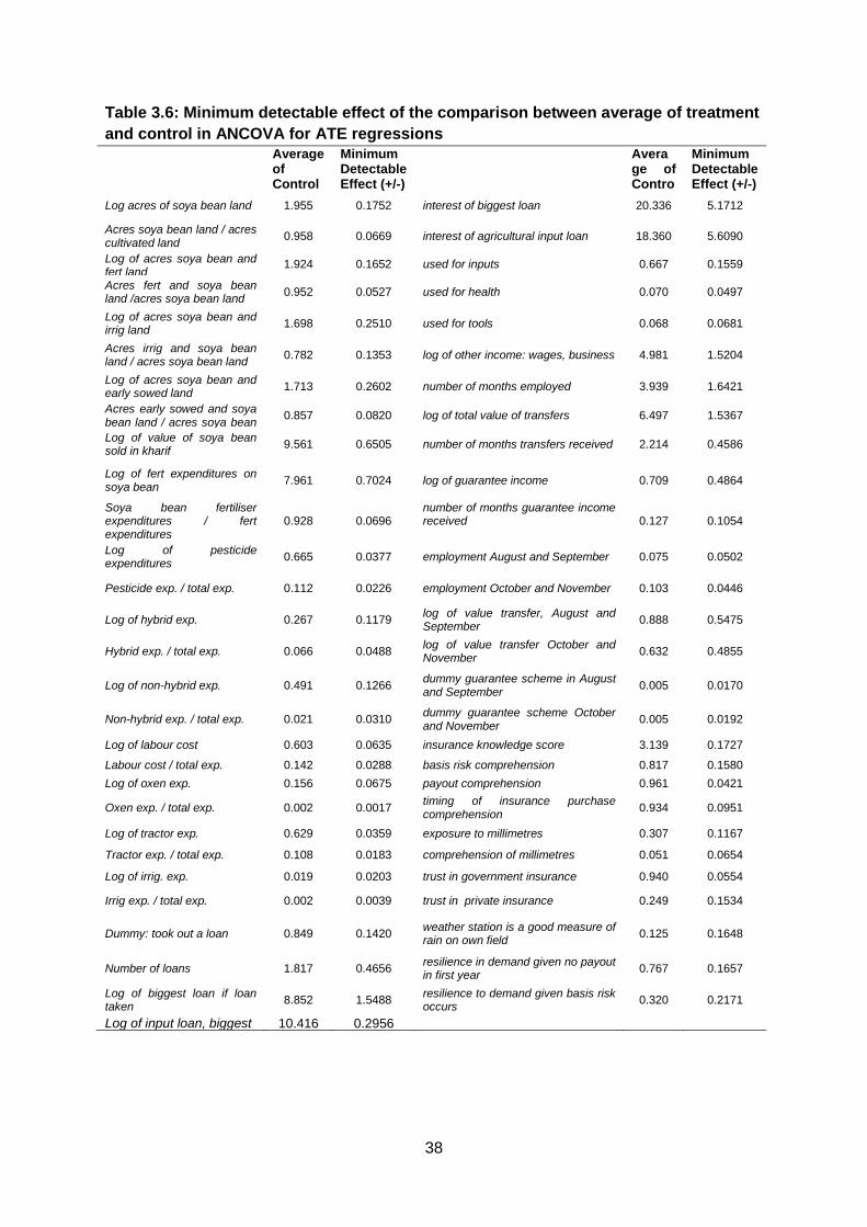
38

Table 3.6: Minimum detectable effect of the comparison between average of treatment

and control in ANCOVA for ATE regressions

Average of Control

Minimum Detectable Effect (+/-)

Average of Control

Minimum Detectable Effect (+/-)

Log acres of soya bean land 1.955 0.1752 interest of biggest loan 20.336 5.1712

Acres soya bean land / acres cultivated land

0.958 0.0669 interest of agricultural input loan 18.360 5.6090

Log of acres soya bean and fert land

1.924 0.1652 used for inputs 0.667 0.1559

Acres fert and soya bean land /acres soya bean land

0.952 0.0527 used for health 0.070 0.0497

Log of acres soya bean and irrig land

1.698 0.2510 used for tools 0.068 0.0681

Acres irrig and soya bean land / acres soya bean land

0.782 0.1353 log of other income: wages, business 4.981 1.5204

Log of acres soya bean and early sowed land

1.713 0.2602 number of months employed 3.939 1.6421

Acres early sowed and soya bean land / acres soya bean lan

0.857 0.0820 log of total value of transfers 6.497 1.5367

Log of value of soya bean sold in kharif

9.561 0.6505 number of months transfers received 2.214 0.4586

Log of fert expenditures on soya bean

7.961 0.7024 log of guarantee income 0.709 0.4864

Soya bean fertiliser expenditures / fert expenditures

0.928 0.0696 number of months guarantee income received

0.127 0.1054

Log of pesticide expenditures

0.665 0.0377 employment August and September 0.075 0.0502

Pesticide exp. / total exp. 0.112 0.0226 employment October and November 0.103 0.0446

Log of hybrid exp. 0.267 0.1179 log of value transfer, August and September

0.888 0.5475

Hybrid exp. / total exp. 0.066 0.0488 log of value transfer October and November

0.632 0.4855

Log of non-hybrid exp. 0.491 0.1266 dummy guarantee scheme in August and September

0.005 0.0170

Non-hybrid exp. / total exp. 0.021 0.0310 dummy guarantee scheme October and November

0.005 0.0192

Log of labour cost 0.603 0.0635 insurance knowledge score 3.139 0.1727

Labour cost / total exp. 0.142 0.0288 basis risk comprehension 0.817 0.1580

Log of oxen exp. 0.156 0.0675 payout comprehension 0.961 0.0421

Oxen exp. / total exp. 0.002 0.0017 timing of insurance purchase comprehension

0.934 0.0951

Log of tractor exp. 0.629 0.0359 exposure to millimetres 0.307 0.1167

Tractor exp. / total exp. 0.108 0.0183 comprehension of millimetres 0.051 0.0654

Log of irrig. exp. 0.019 0.0203 trust in government insurance 0.940 0.0554

Irrig exp. / total exp. 0.002 0.0039 trust in private insurance 0.249 0.1534

Dummy: took out a loan 0.849 0.1420 weather station is a good measure of rain on own field

0.125 0.1648

Number of loans 1.817 0.4656 resilience in demand given no payout in first year

0.767 0.1657

Log of biggest loan if loan taken

8.852 1.5488 resilience to demand given basis risk occurs

0.320 0.2171

Log of input loan, biggest 10.416 0.2956

39

6.2.1 Understanding variations in take-up: changes in attitudes and perceptions

The provision of a new product to a target population that is unfamiliar about its key

characteristics can largely hinder its demand. As mentioned above, during the first year of

implementation, we encountered a low take-up for the product. However, as the introduction

of a new insurance product can take time to take root in a rural population like the one in our

sample, a significant impact on the knowledge and attitudes of farmers towards insurance

can be indicative of a potential future impact on demand. In this section, we thus investigate

the impact of offering insurance and of the three randomised treatments (new weather

station, intensive training and distribution of price discount vouchers) on different measures

of knowledge about insurance, attitudes towards various aspects of our product such as

basis risk and trust in insurance providers.

Table 3.7 provides the results from a series of regressions measuring the impact of (i)

offering insurance (ITT) and (ii) purchase of insurance (ATE), on a set of trust and

knowledge variables of interest. Each row corresponds to one variable, and each column

corresponds to a different regression with the same dependent variable. For example, the

first variable, insurance knowledge score, is the subject of two regressions: the ITT impact of

offering insurance on the insurance knowledge score, and the ATT impact of insurance

purchase on this score. The relevant coefficients from these two regressions are shown in

columns 1 and 3, respectively, followed by their standard errors and corresponding number

of observations. All regressions use an ANCOVA estimator.10

The insurance knowledge score takes a value from 0 to 5, depending on the number of

individual questions that a respondent answered correctly. These questions are shown as

the next five variables (rows) in Table 3.7, and range from comprehension of the properties

of basis risk to comprehension of the concept of millimetres, each of which takes a value of

zero or one. The rest of the variables are also binary. The last two variables are based on

hypothetical questions on whether a household would buy insurance, given that no payouts

were made in the first year. In the first case, a value of one indicates that a household would

do so in the most basic scenario. In the second, a value of one indicates that a household is

still willing to purchase insurance even if it received poor rain.

The results in Table 3.7 indicate that the offer of insurance had a significant effect on

knowledge and trust, while the purchase of insurance increased comprehension of only

certain aspects of our knowledge tests. Now, the ITT effect of offering insurance actually

captures the average effect of a set of various treatments. Therefore, we want to understand

the specific mechanisms through which certain treatments can increase knowledge, positive

attitudes towards the product and trust in the provider. Specifically, we want to know how

each different arm of our treatments influenced households. Furthermore, we wish to

examine if the interaction of certain treatments created an added incentive to the households

to learn from the training modules.

In Tables 3.8a and 3.8b, we examine the ATE impact of each treatment arm on six of the

dependent variables presented in Table 3.7. In Table 3.8a, the treatments are new weather

10 As a word of caution, the F statistic in the first stage of the ATE specifications is not very high (of around 5,

depending on the specification), which hints at a weak instrument problem. This is to be expected since uptake

was very low, which leads into the low power issue discussed above.

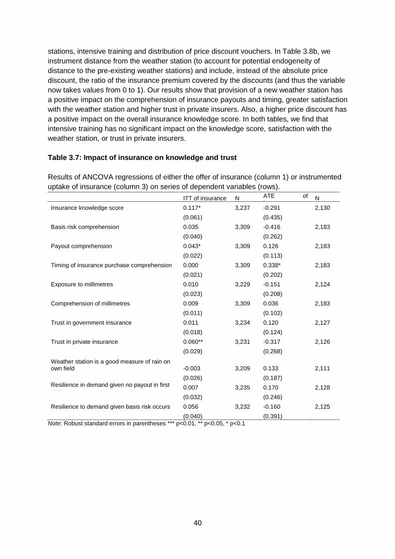
40

stations, intensive training and distribution of price discount vouchers. In Table 3.8b, we

instrument distance from the weather station (to account for potential endogeneity of

distance to the pre-existing weather stations) and include, instead of the absolute price

discount, the ratio of the insurance premium covered by the discounts (and thus the variable

now takes values from 0 to 1). Our results show that provision of a new weather station has

a positive impact on the comprehension of insurance payouts and timing, greater satisfaction

with the weather station and higher trust in private insurers. Also, a higher price discount has

a positive impact on the overall insurance knowledge score. In both tables, we find that

intensive training has no significant impact on the knowledge score, satisfaction with the

weather station, or trust in private insurers.

Table 3.7: Impact of insurance on knowledge and trust

Results of ANCOVA regressions of either the offer of insurance (column 1) or instrumented

uptake of insurance (column 3) on series of dependent variables (rows).

ITT of insurance N ATE of insurance

N

Insurance knowledge score 0.117* 3,237 -0.291 2,130

(0.061) (0.435)

Basis risk comprehension 0.035 3,309 -0.416 2,183

(0.040) (0.262)

Payout comprehension 0.043* 3,309 0.126 2,183

(0.022) (0.113)

Timing of insurance purchase comprehension 0.000 3,309 0.338* 2,183

(0.021) (0.202)

Exposure to millimetres 0.010 3,229 -0.151 2,124

(0.023) (0.208)

Comprehension of millimetres 0.009 3,309 0.036 2,183

(0.011) (0.102)

Trust in government insurance 0.011 3,234 0.120 2,127

(0.018) (0.124)

Trust in private insurance 0.060** 3,231 -0.317 2,126

(0.029) (0.268)

Weather station is a good measure of rain on own field -0.003 3,209 0.133 2,111

(0.026) (0.187) Resilience in demand given no payout in first year

0.007 3,235 0.170 2,128

(0.032) (0.246)

Resilience to demand given basis risk occurs 0.056 3,232 -0.160 2,125

(0.040) (0.391)

Note: Robust standard errors in parentheses *** p<0.01, ** p<0.05, * p<0.1

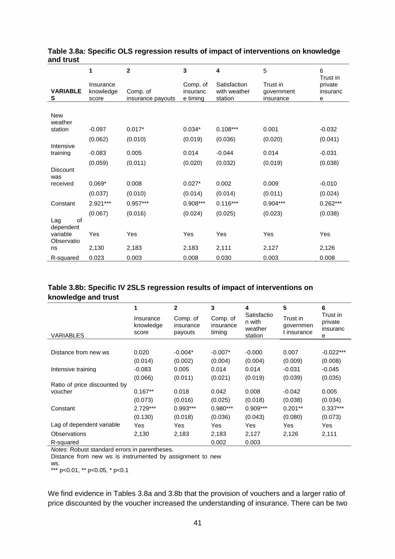
41

Table 3.8a: Specific OLS regression results of impact of interventions on knowledge and trust

1 2 3 4 5 6

VARIABLES

Insurance knowledge score

Comp. of insurance payouts

Comp. of insurance timing

Satisfaction with weather station

Trust in government insurance

Trust in private insurance

New weather station -0.097 0.017* 0.034* 0.108*** 0.001 -0.032

(0.062) (0.010) (0.019) (0.036) (0.020) (0.041) Intensive training -0.083 0.005 0.014 -0.044 0.014 -0.031

(0.059) (0.011) (0.020) (0.032) (0.019) (0.038) Discount was received 0.069* 0.008 0.027* 0.002 0.009 -0.010

(0.037) (0.010) (0.014) (0.014) (0.011) (0.024)

Constant 2.921*** 0.957*** 0.908*** 0.116*** 0.904*** 0.262***

(0.067) (0.016) (0.024) (0.025) (0.023) (0.038) Lag of dependent variable Yes Yes Yes Yes Yes Yes Observations 2,130 2,183 2,183 2,111 2,127 2,126

R-squared 0.023 0.003 0.008 0.030 0.003 0.008

Table 3.8b: Specific IV 2SLS regression results of impact of interventions on

knowledge and trust

1 2 3 4 5 6

VARIABLES

Insurance knowledge score

Comp. of insurance payouts

Comp. of insurance timing

Satisfaction with weather station

Trust in government insurance

Trust in private insurance

Distance from new ws 0.020 -0.004* -0.007* -0.000 0.007 -0.022***

(0.014) (0.002) (0.004) (0.004) (0.009) (0.008)

Intensive training -0.083 0.005 0.014 0.014 -0.031 -0.045

(0.066) (0.011) (0.021) (0.019) (0.039) (0.035) Ratio of price discounted by voucher 0.167** 0.018 0.042 0.008 -0.042 0.005

(0.073) (0.016) (0.025) (0.018) (0.038) (0.034)

Constant 2.729*** 0.993*** 0.980*** 0.909*** 0.201** 0.337***

(0.130) (0.018) (0.036) (0.043) (0.080) (0.073)

Lag of dependent variable Yes Yes Yes Yes Yes Yes

Observations 2,130 2,183 2,183 2,127 2,126 2,111

R-squared 0.002 0.003

Notes: Robust standard errors in parentheses. Distance from new ws is instrumented by assignment to new ws. *** p<0.01, ** p<0.05, * p<0.1

We find evidence in Tables 3.8a and 3.8b that the provision of vouchers and a larger ratio of

price discounted by the voucher increased the understanding of insurance. There can be two

42

reasons for this. First, the provision of a voucher created higher incentives to pay more

attention during the training session. Second, people who received vouchers were more

likely to purchase insurance and therefore were able to learn about insurance through this

process, the so-called learning-by-doing.11 Some suggestive evidence of this effect can be

seen in Table 3.7, where we find that households who purchased insurance had a higher

comprehension of a number of components in our score. In Tables 3.8a and 3.8b, we further

find this effect amongst the households with new weather stations and closer distance to a

weather station. We also find that households that had insurance referenced to a new

weather station were significantly more satisfied with how their rain was measured.

Furthermore, households that were further away from weather stations had significantly

lower comprehension of insurance payouts and timing and lower trust in private insurance.

In addition, we want to better understand why intensive training was not beneficial in

increasing insurance understanding in our sample. We must not forget, however, that

intensive training was in fact an additional two hours of training on top of an initial two-hour

basic training session provided to all households who were offered insurance. Unfortunately,

we do not have the ability to measure the exact impact of this basic two-hour training as it

perfectly correlates with the offering of insurance (all households that were offered basic

training were at the same time offered insurance). In Table 3.9, we present a set of

regressions on the same set of dependent variables, where the relevant independent

variables are the offer of insurance, and the offer of insurance interacted with other

treatments (intensive training, a new weather station, or insurance price discount). The first

coefficient is the marginal effect of just offering insurance without any further treatments,

while the second coefficient captures the additional effect of providing the other treatments.

The problem with this is that in the context of selling such a product, knowledge can be

increased by simply offering insurance if the target sample sought out information to make a

purchase decision. While we cannot directly measure how much effort a household put into

gathering information outside of training, the overall demand for households who did not

receive any other treatments is very low. Therefore, we speculate that the impact of

marketing on seeking out information explains a small fraction of what we see. Specifically,

we see that the overall knowledge score was significantly higher when basic training was

offered with insurance than when neither was provided. The size of the effect is higher than

that of an offer of a price discount voucher presented in row three of Table 3.8a. Therefore,

we take this as weak evidence to point out that while extra training is not helpful, basic

training might be impacting knowledge about insurance. Again, however, this effect is

unfortunately technically indistinguishable from the marketing effect, so these results need to

be seen with caution.

11 The effects we observe could be potentially driven by a behavioural response of the recipients to receiving a

voucher, where the voucher may serve as a reminder that repeatedly draws the individual’s attention to the topic

of insurance. Unfortunately, our design does not allow us to separate this effect from the learning-by-doing

mentioned above.

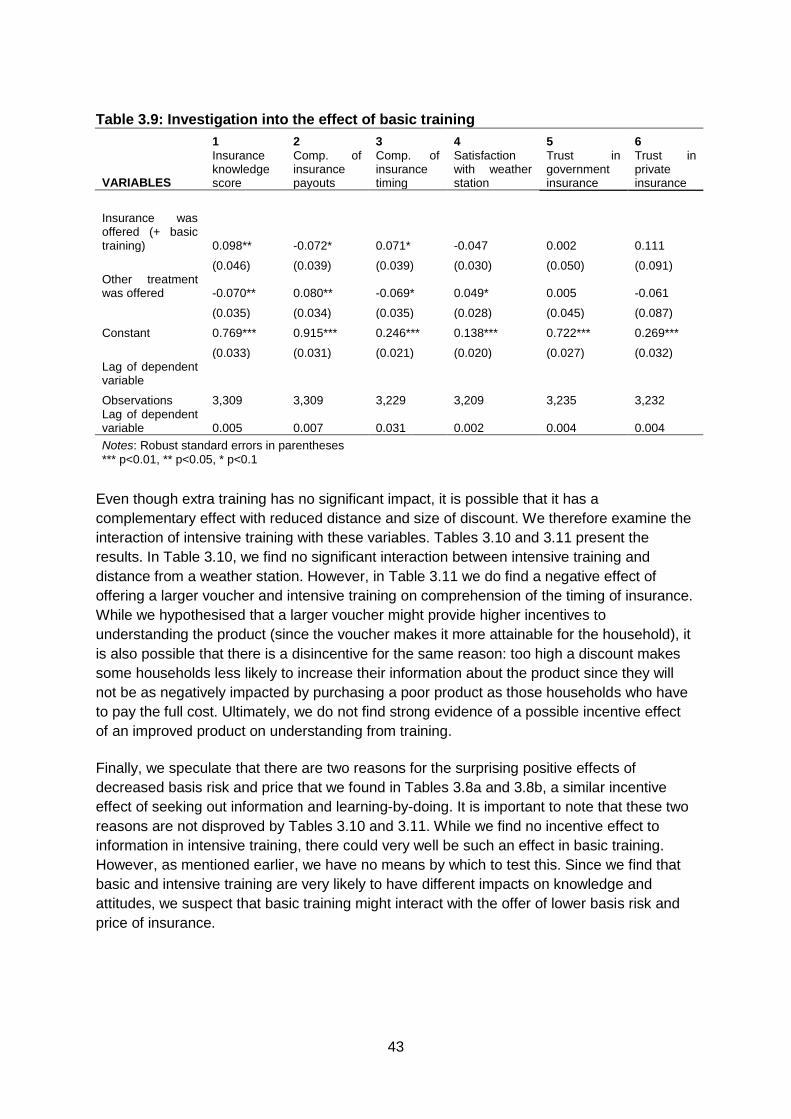
43

Table 3.9: Investigation into the effect of basic training

1 2 3 4 5 6

VARIABLES

Insurance knowledge score

Comp. of insurance payouts

Comp. of insurance timing

Satisfaction with weather station

Trust in government insurance

Trust in private insurance

Insurance was offered (+ basic training) 0.098** -0.072* 0.071* -0.047 0.002 0.111

(0.046) (0.039) (0.039) (0.030) (0.050) (0.091) Other treatment was offered -0.070** 0.080** -0.069* 0.049* 0.005 -0.061

(0.035) (0.034) (0.035) (0.028) (0.045) (0.087)

Constant 0.769*** 0.915*** 0.246*** 0.138*** 0.722*** 0.269***

(0.033) (0.031) (0.021) (0.020) (0.027) (0.032) Lag of dependent variable

Observations 3,309 3,309 3,229 3,209 3,235 3,232 Lag of dependent variable 0.005 0.007 0.031 0.002 0.004 0.004

Notes: Robust standard errors in parentheses

*** p<0.01, ** p<0.05, * p<0.1

Even though extra training has no significant impact, it is possible that it has a

complementary effect with reduced distance and size of discount. We therefore examine the

interaction of intensive training with these variables. Tables 3.10 and 3.11 present the

results. In Table 3.10, we find no significant interaction between intensive training and

distance from a weather station. However, in Table 3.11 we do find a negative effect of

offering a larger voucher and intensive training on comprehension of the timing of insurance.

While we hypothesised that a larger voucher might provide higher incentives to

understanding the product (since the voucher makes it more attainable for the household), it

is also possible that there is a disincentive for the same reason: too high a discount makes

some households less likely to increase their information about the product since they will

not be as negatively impacted by purchasing a poor product as those households who have

to pay the full cost. Ultimately, we do not find strong evidence of a possible incentive effect

of an improved product on understanding from training.

Finally, we speculate that there are two reasons for the surprising positive effects of

decreased basis risk and price that we found in Tables 3.8a and 3.8b, a similar incentive

effect of seeking out information and learning-by-doing. It is important to note that these two

reasons are not disproved by Tables 3.10 and 3.11. While we find no incentive effect to

information in intensive training, there could very well be such an effect in basic training.

However, as mentioned earlier, we have no means by which to test this. Since we find that

basic and intensive training are very likely to have different impacts on knowledge and

attitudes, we suspect that basic training might interact with the offer of lower basis risk and

price of insurance.

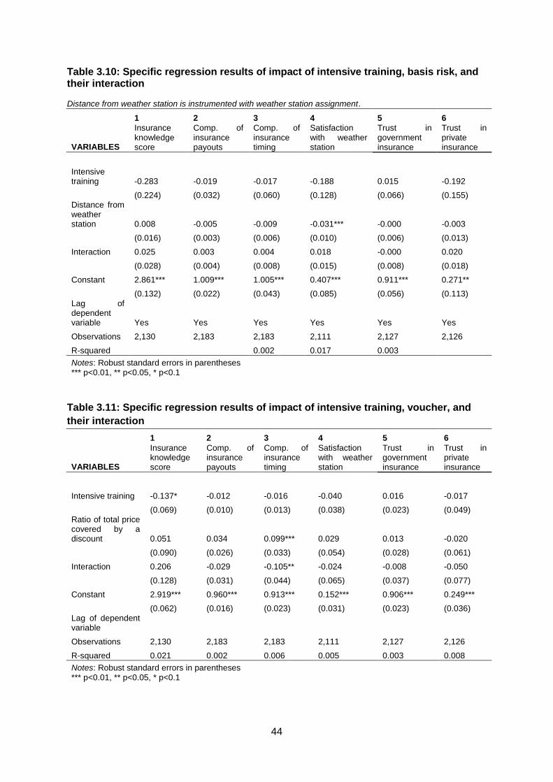
44

Table 3.10: Specific regression results of impact of intensive training, basis risk, and their interaction Distance from weather station is instrumented with weather station assignment.

1 2 3 4 5 6

VARIABLES

Insurance knowledge score

Comp. of insurance payouts

Comp. of insurance timing

Satisfaction with weather station

Trust in government insurance

Trust in private insurance

Intensive training -0.283 -0.019 -0.017 -0.188 0.015 -0.192

(0.224) (0.032) (0.060) (0.128) (0.066) (0.155) Distance from weather station 0.008 -0.005 -0.009 -0.031*** -0.000 -0.003

(0.016) (0.003) (0.006) (0.010) (0.006) (0.013)

Interaction 0.025 0.003 0.004 0.018 -0.000 0.020

(0.028) (0.004) (0.008) (0.015) (0.008) (0.018)

Constant 2.861*** 1.009*** 1.005*** 0.407*** 0.911*** 0.271**

(0.132) (0.022) (0.043) (0.085) (0.056) (0.113) Lag of dependent variable Yes Yes Yes Yes Yes Yes

Observations 2,130 2,183 2,183 2,111 2,127 2,126

R-squared 0.002 0.017 0.003

Notes: Robust standard errors in parentheses *** p<0.01, ** p<0.05, * p<0.1

Table 3.11: Specific regression results of impact of intensive training, voucher, and

their interaction

1 2 3 4 5 6

VARIABLES

Insurance knowledge score

Comp. of insurance payouts

Comp. of insurance timing

Satisfaction with weather station

Trust in government insurance

Trust in private insurance

Intensive training -0.137* -0.012 -0.016 -0.040 0.016 -0.017

(0.069) (0.010) (0.013) (0.038) (0.023) (0.049) Ratio of total price covered by a discount 0.051 0.034 0.099*** 0.029 0.013 -0.020

(0.090) (0.026) (0.033) (0.054) (0.028) (0.061)

Interaction 0.206 -0.029 -0.105** -0.024 -0.008 -0.050

(0.128) (0.031) (0.044) (0.065) (0.037) (0.077)

Constant 2.919*** 0.960*** 0.913*** 0.152*** 0.906*** 0.249***

(0.062) (0.016) (0.023) (0.031) (0.023) (0.036) Lag of dependent variable

Observations 2,130 2,183 2,183 2,111 2,127 2,126

R-squared 0.021 0.002 0.006 0.005 0.003 0.008

Notes: Robust standard errors in parentheses *** p<0.01, ** p<0.05, * p<0.1

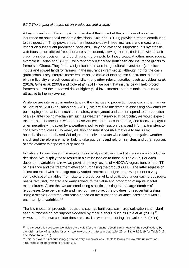
45

6.2.2 The impact of insurance on production and welfare

A key motivation of this study is to understand the impact of the purchase of weather

insurance on household economic decisions. Cole et al. (2011) provide a recent contribution

to this question. They provide treatment households with free insurance and measure its

impact on subsequent production decisions. They find evidence supporting this hypothesis,

with households offered free insurance subsequently sowing more of their land with a cash

crop—a riskier decision—and purchasing more inputs for these crops. Another, more recent,

example is Karlan et al. (2013), who randomly distributed both cash and insurance grants to

farmers in Ghana. They found a significant increase in agricultural investment (chemical

inputs and sowed land) for farmers in the insurance grant group, although not for the cash

grant group. They interpret these results as indicative of binding risk constraints, but non-

binding liquidity or credit constraints. Like many other relevant studies, such as Lybbert et al.

(2010), Gine et al. (2008) and Cole et al. (2011), we posit that insurance will help protect

farmers against the increased risk of higher yield investments and thus make them more

attractive to the risk averse.

While we are interested in understanding the changes to production decisions in the manner

of Cole et al. (2011) or Karlan et al. (2013), we are also interested in assessing how other ex

post coping mechanisms such as transfers, employment and credit respond to the adoption

of an ex ante coping mechanism such as weather insurance. In particular, we would expect

that for those households who purchase WII (weather index insurance) and receive a payout

when negatively impacted by a weather shock to rely less on loans and informal transfers to

cope with crop losses. However, we also consider it possible that due to basis risk

households that purchased WII might not receive payouts when facing a negative weather

shock and therefore are more likely to take out loans and rely on transfers and other sources

of employment to cope with crop losses.

In Table 3.12, we present the results of our analysis of the impact of insurance on production

decisions. We display these results in a similar fashion to those of Table 3.7. For each

dependent variable in a row, we provide the key results of ANCOVA regressions on the ITT

of insurance and the treatment effect of purchasing the product (ATE). The latter regression

is instrumented with the exogenously-varied treatment assignments. We present a very

complete set of variables, from size and proportion of land cultivated under cash crops (soya

bean), fertilised, irrigated and early sowed, to the value and proportion of inputs in total

expenditures. Given that we are conducting statistical testing over a large number of

hypotheses (one per variable and method), we correct the p-values for sequential testing

using a simple Bonferroni correction based on the number of variables considered within

each family of variables.12

The low impact on production decisions such as fertilisers, cash crop cultivation and hybrid

seed purchases do not support evidence by other authors, such as Cole et al. (2011).13

However, before we consider these results, it is worth mentioning that Cole et al. (2011)

12 To conduct this correction, we divide the p-value for the treatment coefficient in each of the specifications by

the total number of variables for which we are conducting tests in that table (25 for Table 3.12, six for Table 3.13,

and 15 for Table 3.15). 13 This is, however, not surprising, given the very low power of our tests following the low take-up rates, as

discussed at the beginning of Section 6.1.

46

gave away insurance that covered, on an average, 1 hectare of land, while an insured

household in our sample purchased, on an average, coverage for only half an acre (about a

fourth of a hectare). Furthermore, the average cultivated land of the sample of Cole et al.

(2011) was 5 acres, while it was a little over 8 acres in our sample. Therefore, the insurance

purchased in our sample constitutes no more than a test-run for households, while the

insurance given by Cole et al. (2011) to their sample covered a significant proportion of their

agricultural production. Hence, while the mechanism of insurance is similar, one should not

necessarily expect to have similar results.

Table 3.13a gives an indication of the impact of insurance offer and purchase on credit

decisions. Our module on credit asked households whether they took a loan, how many

loans they took and a few specifics about their largest loan such as size, interest rate and

purpose. We find that the offer of insurance did not have a detectable impact over any of

these credit measures.

However, we do find that the purchase of insurance resulted in the taking of more loans (as

measured by the ATT specification). We do not have data on the exact timing, type or size of

these loans, which makes it hard to draw conclusions about the exact mechanisms behind

this effect. Regardless, the increase in the number of loans for households that purchased

insurance is interesting. It is possible, for example, that households that purchased

insurance took out very small loans to pay for it. If this were the case, we speculate that the

number of loans should vary with the cost of insurance. In column 1 of Table 3.13b, we add

a variable on the total amount of money spent on insurance by a household to the ATE

regressions shown in Table 3.13a and report the regression results for only this additional

variable. We do not find any significant effects. Another possibility is that, since very few

households that purchased insurance received payouts (14 out of 151), some households

may have needed to take out loans to deal with negative basis risk. To test for this, we add a

dummy variable indicating whether a payout occurred to the ATE specifications in Table

3.13a and report only these additional results (in column 3 of Table 3.13b). We find no

support for our hypothesis, although we should again note the power limitations discussed

above.

In the districts of Bhopal, Ujjain and Dewas, the purchase of government insurance is tied to

government loans for inputs. Therefore, it is possible that households taking government

loans satisfy totally or partially their demand for insurance as government insurance comes

with the loans.14 Therefore, in Table 3.14 we present results on the impact of insurance offer

(ITT) and purchase (ATE) on the demand for insured government loans and on the demand

for stand-alone insurance. While the offer of insurance does not have a significant effect,

households that do purchase insurance are less likely to take out government loans with

insurance. One possibility is that households that purchase insurance are taking smaller

loans for inputs, as opposed to one larger government-insured loan. In any case, this

substitutability between government loans and the HDFC product is to be expected.

However, since we ask households about how many government loans they took out in the

past 12 months in January 2012, we cannot strongly conclude whether the substitutability

happened during kharif 2011 or during the dry season of 2012.

14 As shown in Table 1.1, the proportion of households with access to agricultural loans is more than 90 per cent, with presumably a large number of cases being subsided loans linked to government insurance.

47

In Table 3.15a, we consider the impact of insurance on household transfers and other

sources of income such as wage labour. We label as guarantee scheme the national income

scheme that provides cash for labour to impoverished households. Furthermore, we define

transfers as either educational transfers, donations, gifts, inheritance and dowry from family

members, village members, or local, state and federal entities. We find that households that

were offered insurance received significantly more total transfers in October and November

after the end of the harvest.

Looking at the size of the ATE coefficients of insurance purchase, which are also positive

and of a relatively high magnitude (although not statistically significant), we wondered if this

variable was just capturing HDFC payouts, which would be the case if payouts were

reported by the households as part of transfers. However, out of the 14 households who

received payouts, the reported transfers were not close in value to the HDFC payouts. An

alternative explanation would be that households that received payouts were more willing to

send gifts and donations to other households. A naïve test for such a hypothesis could be to

see whether households in villages where payouts were made were more likely to receive

transfers. In Table 3.15b, we test this by including a dummy equal to one if a household was

in a village where payouts were made, and report the coefficient for this added variable. We

find no statistically significant effect on any of the dependent variables in Table 3.15a.

In terms of other potential mechanisms at play, it could be possible that offering insurance,

with its many training events that brought the village together to discuss overall coping

mechanisms, made each household more aware of the risks of other households and, in

turn, increased transfers to those in need in the aftermath of the rainy season. Alternatively,

the offering of insurance may have given rise to other informal insurance arrangements

between households. However, as we do not count with any evidence or statistical power to

properly distinguish between any of these mechanisms, this discussion is only speculative.

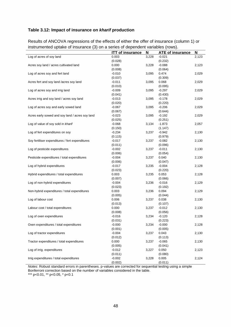
48

Table 3.12: Impact of insurance on kharif production

Results of ANCOVA regressions of the effects of either the offer of insurance (column 1) or

instrumented uptake of insurance (3) on a series of dependent variables (rows).

ITT of insurance N ATE of insurance N Log of acres of soy land 0.003 3,228 -0.021 2,123

(0.028) (0.232)

Acres soy land / acres cultivated land 0.000 3,228 -0.088 2,123

(0.008) (0.064)

Log of acres soy and fert land -0.010 3,095 0.474 2,029

(0.037) (0.309)

Acres fert and soy land /acres soy land -0.011 3,095 0.068 2,029

(0.010) (0.095)

Log of acres soy and irrig land -0.009 3,095 -0.297 2,029

(0.041) (0.430)

Acres irrig and soy land / acres soy land -0.013 3,095 -0.178 2,029

(0.020) (0.220)

Log of acres soy and early sowed land -0.067 3,095 -0.206 2,029

(0.067) (0.644)

Acres early sowed and soy land / acres soy land -0.023 3,095 -0.192 2,029

(0.025) (0.251)

Log of value of soy sold in kharif -0.068 3,134 -1.873 2,057

(0.150) (1.147)

Log of fert expenditures on soy -0.234 3,237 -0.942 2,130

(0.115) (0.979)

Soy fertiliser expenditures / fert expenditures -0.017 3,237 -0.082 2,130

(0.011) (0.096)

Log of pesticide expenditures -0.002 3,237 -0.011 2,130

(0.006) (0.054)

Pesticide expenditures / total expenditures -0.004 3,237 0.040 2,130

(0.006) (0.047)

Log of hybrid expenditures -0.017 3,235 -0.004 2,128

(0.023) (0.220)

Hybrid expenditures / total expenditures 0.003 3,235 0.053 2,128

(0.007) (0.066)

Log of non-hybrid expenditures -0.004 3,236 -0.016 2,129

(0.023) (0.192)

Non-hybrid expenditures / total expenditures 0.003 3,236 0.094 2,129

(0.005) (0.044)

Log of labour cost 0.006 3,237 0.038 2,130

(0.013) (0.107)

Labour cost / total expenditures 0.000 3,237 -0.012 2,130

(0.008) (0.056)

Log of oxen expenditures -0.016 3,234 -0.120 2,128

(0.031) (0.223)

Oxen expenditures / total expenditures -0.000 3,234 -0.000 2,128

(0.001) (0.005)

Log of tractor expenditures -0.004 3,237 0.043 2,130

(0.012) (0.113)

Tractor expenditures / total expenditures 0.000 3,237 -0.065 2,130

(0.005) (0.041)

Log of irrig. expenditures -0.012 3,227 0.050 2,123

(0.011) (0.080)

Irrig expenditures / total expenditures -0.002 3,228 0.005 2,124

(0.002) (0.011)

Notes: Robust standard errors in parentheses. p-values are corrected for sequential testing using a simple Bonferroni correction based on the number of variables considered in the table. *** p<0.01, ** p<0.05, * p<0.1

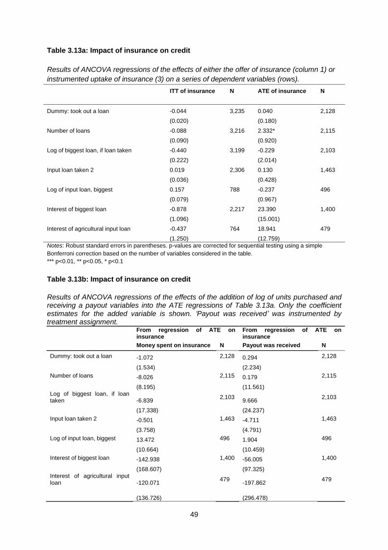
49

Table 3.13a: Impact of insurance on credit

Results of ANCOVA regressions of the effects of either the offer of insurance (column 1) or

instrumented uptake of insurance (3) on a series of dependent variables (rows).

ITT of insurance N ATE of insurance N

Dummy: took out a loan -0.044 3,235 0.040 2,128

(0.020) (0.180)

Number of loans -0.088 3,216 2.332* 2,115

(0.090) (0.920)

Log of biggest loan, if loan taken -0.440 3,199 -0.229 2,103

(0.222) (2.014)

Input loan taken 2 0.019 2,306 0.130 1,463

(0.036) (0.428)

Log of input loan, biggest 0.157 788 -0.237 496

(0.079) (0.967)

Interest of biggest loan -0.878 2,217 23.390 1,400

(1.096) (15.001)

Interest of agricultural input loan -0.437 764 18.941 479

(1.250) (12.759)

Notes: Robust standard errors in parentheses. p-values are corrected for sequential testing using a simple

Bonferroni correction based on the number of variables considered in the table.

*** p<0.01, ** p<0.05, * p<0.1

Table 3.13b: Impact of insurance on credit

Results of ANCOVA regressions of the effects of the addition of log of units purchased and receiving a payout variables into the ATE regressions of Table 3.13a. Only the coefficient estimates for the added variable is shown. ‘Payout was received’ was instrumented by treatment assignment.

From regression of ATE on insurance

From regression of ATE on insurance

Money spent on insurance N Payout was received N

Dummy: took out a loan -1.072 2,128 0.294 2,128

(1.534) (2.234)

Number of loans -8.026 2,115 0.179 2,115

(8.195) (11.561) Log of biggest loan, if loan taken -6.839

2,103 9.666

2,103

(17.338) (24.237)

Input loan taken 2 -0.501 1,463 -4.711 1,463

(3.758) (4.791)

Log of input loan, biggest 13.472 496 1.904 496

(10.664) (10.459)

Interest of biggest loan -142.938 1,400 -56.005 1,400

(168.607) (97.325) Interest of agricultural input loan -120.071

479 -197.862

479

(136.726)

(296.478)

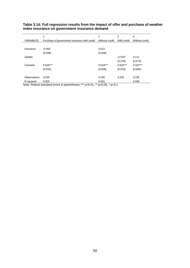
50

Table 3.14: Full regression results from the impact of offer and purchase of weather index insurance on government insurance demand

1 2 3 4

VARIABLES Purchase of government insurance with credit Without credit With credit Without credit

Insurance -0.056 0.012

(0.039) (0.009)

Uptake -0.516* 0.111

(0.278) (0.073)

Constant 0.646*** 0.019*** 0.632*** 0.022***

(0.032) (0.006) (0.023) (0.005)

Observations 3,235 3,235 3,235 3,235

R-squared 0.003 0.001 0.006

Note: Robust standard errors in parentheses *** p<0.01, ** p<0.05, * p<0.1

51

Table 3.15a: Impact of insurance on transfers, employment and other sources of

income

Results of ANCOVA regressions of the effects of either the offer of insurance (column 1) or

instrumented uptake of insurance (3) on a series of dependent variables (rows).

ITT of insurance N ATE of insurance N

Log of other income: wages, business -0.141 3,237 0.591 2,130

(0.273) (2.559)

Number of months employed -0.308 3,237 0.444 2,130

(0.306) (2.884)

Log of total value of transfers -0.012 3,237 5.499 2,130

(0.487) (4.140)

Number of months transfers received 0.215 3,237 1.398 2,130

(0.155) (1.460)

Log of guarantee income 0.098 3,237 -1.161 2,130

(0.146) (1.393)

Number of months guarantee income received 0.006 3,237 -0.193 2,130

(0.033) (0.288)

Employment August and September -0.009 3,237 0.109 2,130

(0.008) (0.064)

Employment October and November -0.008 3,237 -0.004 2,130

(0.009) (0.068)

Log of value transfer, August and September 0.092 3,237 0.436 2,130

(0.166) (1.148)

Log of donations and gifts, August and September -0.008 3,237 -0.218 2,130

(0.045) (0.327)

Log of educational transfers, August and September -0.005 3,237 1.139 2,130

(0.157) (0.959)

Log of value transfer, October and November 0.258* 3,237 1.248 2,130

(0.091) (1.058)

Log of donations and gifts, October and November 0.125 3,237 0.952 2,130

(0.046) (0.705)

Log of educational transfers, October and November 0.041 3,237 0.805 2,129

(0.059) (0.568)

Dummy guarantee scheme in August and September -0.005 3,237 0.019 2,130

(0.003) (0.024)

Dummy guarantee scheme in October and November -0.001 3,237 0.016 2,130

(0.003) (0.033)

Notes: Robust standard errors in parentheses. p-values are corrected for sequential testing using a simple Bonferroni correction based on the number of variables considered in the table. *** p<0.01, ** p<0.05, * p<0.1

52

Table 3.15b: Impact of insurance on transfers, employment and other sources of

income

Results of ANCOVA regression of the effects of the addition of a dummy variable capturing

whether a payout was made in the village of a household into the ATE regressions of Table

3.15a. Only the coefficient estimate for the added variable is shown. ‘Dummy, payouts made

in the village’ is instrumented by the treatment assignment.

From regression of ATE on insurance

Dummy, payouts made in the village N

Log of other income: wages, business -3.812 2,130

(5.040)

Number of months employed -3.948 2,130

(5.066)

Log of total value of transfers 3.343 2,130

(6.751)

Number of months transfers received -2.785 2,130

(3.044)

Log of guarantee income -0.138 2,130

(1.954)

Number of months guarantee income received -0.048 2,130

(0.398)

Employment August and September -0.187 2,130

(0.206)

Employment October and November -0.084 2,130

(0.148)

Log of value transfer, August and September -3.866 2,130

(4.127)

Log of donations and gifts, August and September 0.643 2,130

(0.821)

Log of educational transfers, August and September -2.638 2,130

(2.806)

Log of value transfer, October and November -4.553 2,130

(4.381)

Log of donations and gifts, October and November -1.097 2,130

(1.412)

Log of educational transfers, October and November -1.333 2,129

(1.464)

Dummy guarantee scheme in August and September -0.026 2,130

(0.042)

Dummy guarantee scheme in October and November -0.008 2,130

(0.031)

53

6.3 The longer run impact of offering insurance on demand

We now turn to the effect of the marketing interventions on take-up in 2012, the second

season of sales for the index insurance product. As described above, in 2012 we again

offered price discounts, randomised at the village level (to sampled and non-sampled

households), but left the other treatments unchanged: no new weather stations were

installed and no additional training sessions were conducted.

Table 3.16 presents ITT regression specifications for the second season of index insurance

sales. The price of the insurance policy is again strongly significant in predicting demand.

The distance to the weather station is also strongly associated with purchases in the

subsample of villages served by new stations, though only weakly associated with demand

in the full sample, arguably due to a lack of power from low take-up. Interestingly, the effect

of training seems to fade over time: although receiving intensive training significantly

increased demand in the season immediately following training, it had no significant effect on

demand in 2012. This confirms the finding in the previous section that insurance literacy

training did not seem to have a lasting effect on knowledge about the insurance product

during the midline survey.

In Table 3.17, we include the discount received in 2011 as an additional control, but find no

effect on demand. This is surprising given the results in previous sections, which suggested

that households that had received a subsidy had a much better understanding of the

insurance product. Also, this result does not seem to support the existence of a

discouragement (encouragement) effect of having received a higher (lower) discount in the

past season. In sum, the results suggest that insurance literacy training and subsidies have

an immediate, but not a sustained, effect on demand.

In Table 3.18, we test the relationship between an individual’s experience with weather

insurance in 2011 and demand in 2012. We find that prior experience of insurance is a

strong predictor of demand. While purchasing insurance in 2011 has a small but significant

impact on the demand in 2012 on its own, purchasing insurance in 2011 and receiving a

payout is strongly positively correlated with the decision to purchase insurance in the

subsequent season. However, there seems to be no impact on demand of observing other

households in the village receiving a payout.15,16

15 These results are unreported and are available on request. 16 This pattern closely resembles that found by Stein (2011), and is in contrast to the work of Cole, Stein and

Tobacman (2014) who find that experiencing a payout in the village is the only relevant predictor of future

demand, regardless of individually receiving a payout, and that of Karlan et al. (2012), who find individual as well

as social network spillover effects.

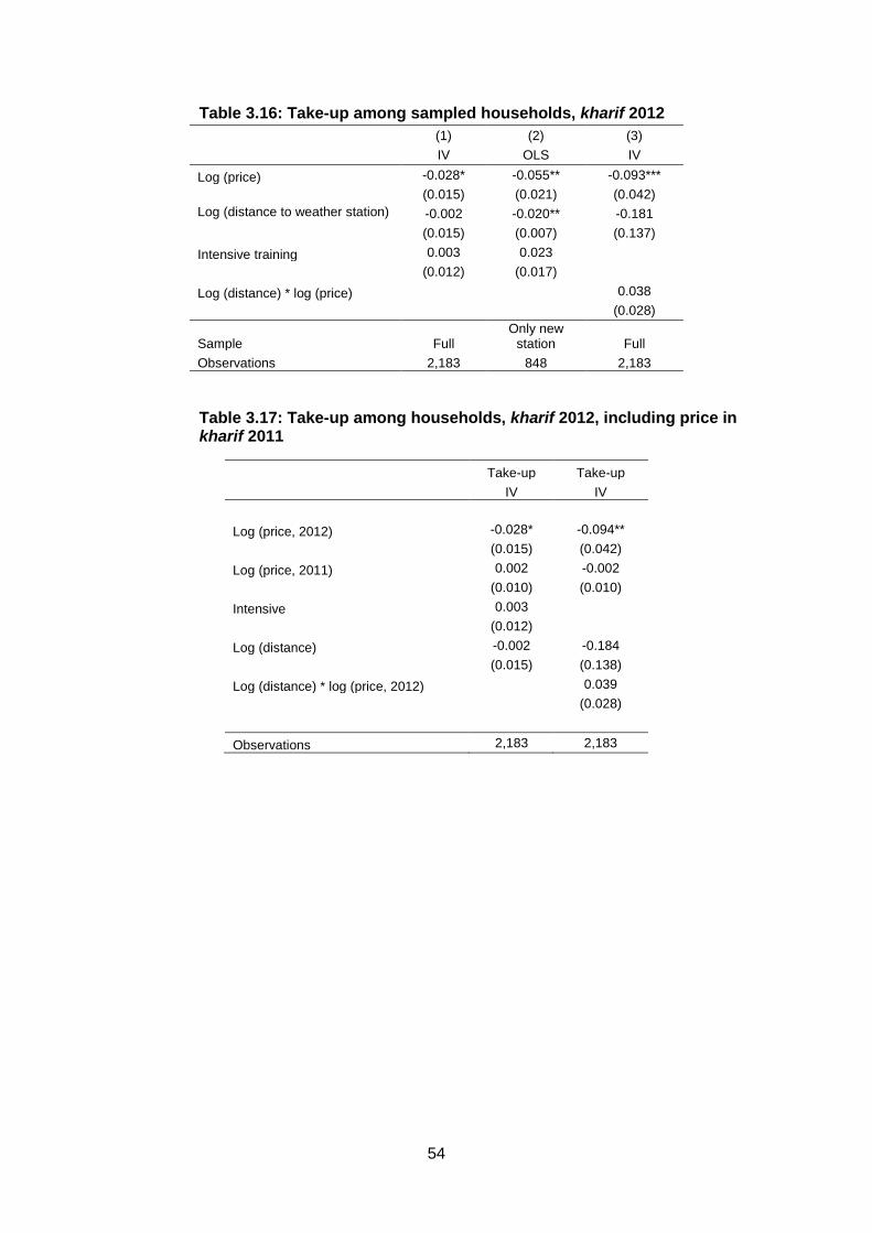
54

Table 3.16: Take-up among sampled households, kharif 2012

(1) (2) (3)

IV OLS IV

Log (price) -0.028* -0.055** -0.093***

(0.015) (0.021) (0.042)

Log (distance to weather station) -0.002 -0.020** -0.181

(0.015) (0.007) (0.137)

Intensive training 0.003 0.023

(0.012) (0.017)

Log (distance) * log (price) 0.038

(0.028)

Sample Full Only new

station Full

Observations 2,183 848 2,183

Table 3.17: Take-up among households, kharif 2012, including price in kharif 2011

Take-up Take-up

IV IV

Log (price, 2012) -0.028* -0.094**

(0.015) (0.042)

Log (price, 2011) 0.002 -0.002

(0.010) (0.010)

Intensive 0.003

(0.012)

Log (distance) -0.002 -0.184

(0.015) (0.138)

Log (distance) * log (price, 2012) 0.039

(0.028)

Observations 2,183 2,183

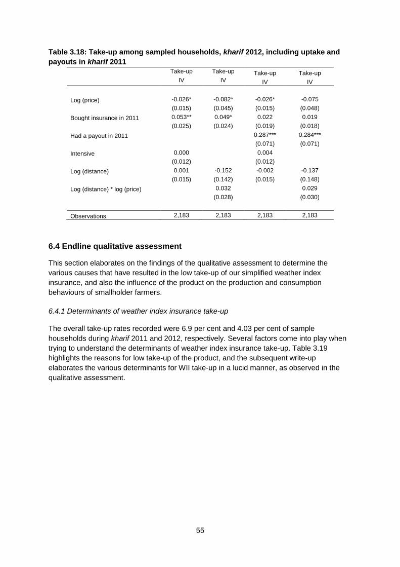
55

Table 3.18: Take-up among sampled households, kharif 2012, including uptake and

payouts in kharif 2011

Take-up Take-up Take-up Take-up

IV IV IV IV

Log (price) -0.026* -0.082* -0.026* -0.075

(0.015) (0.045) (0.015) (0.048)

Bought insurance in 2011 0.053** 0.049* 0.022 0.019

(0.025) (0.024) (0.019) (0.018)

Had a payout in 2011 0.287*** 0.284***

(0.071) (0.071)

Intensive 0.000 0.004

(0.012) (0.012)

Log (distance) 0.001 -0.152 -0.002 -0.137

(0.015) (0.142) (0.015) (0.148)

Log (distance) * log (price) 0.032 0.029

(0.028) (0.030)

Observations 2,183 2,183 2,183 2,183

6.4 Endline qualitative assessment

This section elaborates on the findings of the qualitative assessment to determine the

various causes that have resulted in the low take-up of our simplified weather index

insurance, and also the influence of the product on the production and consumption

behaviours of smallholder farmers.

6.4.1 Determinants of weather index insurance take-up

The overall take-up rates recorded were 6.9 per cent and 4.03 per cent of sample

households during kharif 2011 and 2012, respectively. Several factors come into play when

trying to understand the determinants of weather index insurance take-up. Table 3.19

highlights the reasons for low take-up of the product, and the subsequent write-up

elaborates the various determinants for WII take-up in a lucid manner, as observed in the

qualitative assessment.

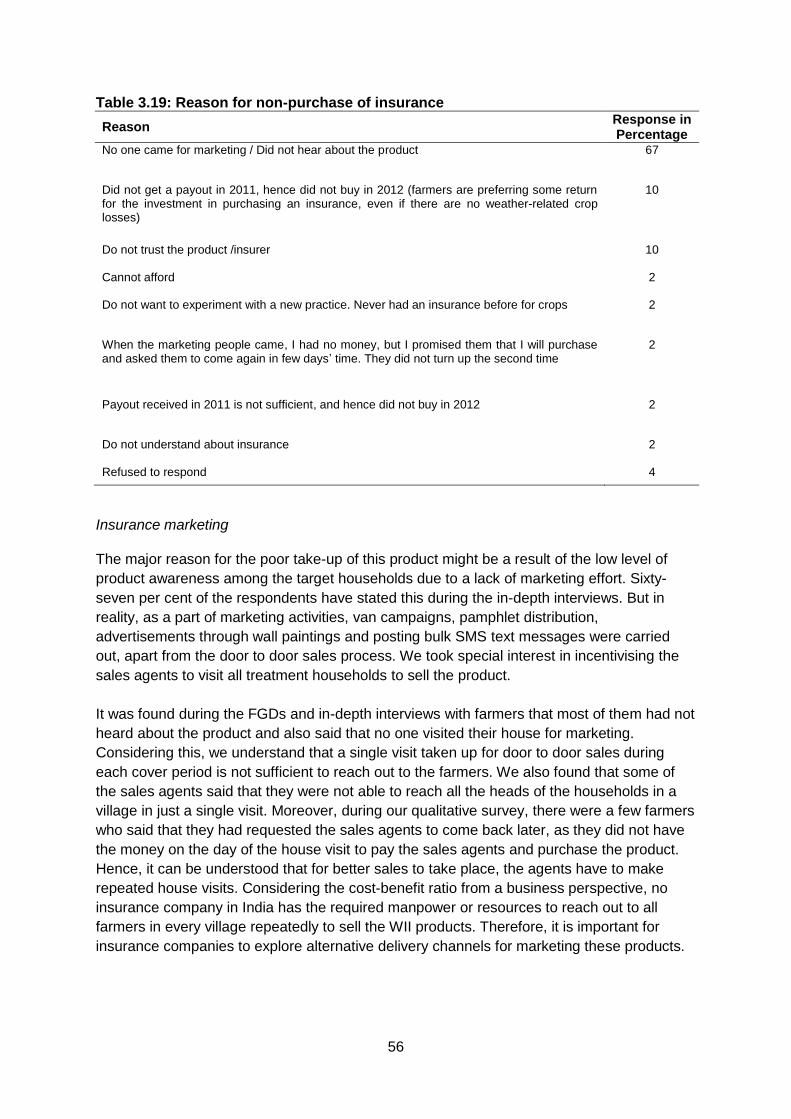
56

Table 3.19: Reason for non-purchase of insurance

Reason Response in Percentage

No one came for marketing / Did not hear about the product 67

Did not get a payout in 2011, hence did not buy in 2012 (farmers are preferring some return for the investment in purchasing an insurance, even if there are no weather-related crop losses)

10

Do not trust the product /insurer 10

Cannot afford 2

Do not want to experiment with a new practice. Never had an insurance before for crops 2

When the marketing people came, I had no money, but I promised them that I will purchase and asked them to come again in few days’ time. They did not turn up the second time

2

Payout received in 2011 is not sufficient, and hence did not buy in 2012 2

Do not understand about insurance 2

Refused to respond 4

Insurance marketing

The major reason for the poor take-up of this product might be a result of the low level of

product awareness among the target households due to a lack of marketing effort. Sixty-

seven per cent of the respondents have stated this during the in-depth interviews. But in

reality, as a part of marketing activities, van campaigns, pamphlet distribution,

advertisements through wall paintings and posting bulk SMS text messages were carried

out, apart from the door to door sales process. We took special interest in incentivising the

sales agents to visit all treatment households to sell the product.

It was found during the FGDs and in-depth interviews with farmers that most of them had not

heard about the product and also said that no one visited their house for marketing.

Considering this, we understand that a single visit taken up for door to door sales during

each cover period is not sufficient to reach out to the farmers. We also found that some of

the sales agents said that they were not able to reach all the heads of the households in a

village in just a single visit. Moreover, during our qualitative survey, there were a few farmers

who said that they had requested the sales agents to come back later, as they did not have

the money on the day of the house visit to pay the sales agents and purchase the product.

Hence, it can be understood that for better sales to take place, the agents have to make

repeated house visits. Considering the cost-benefit ratio from a business perspective, no

insurance company in India has the required manpower or resources to reach out to all

farmers in every village repeatedly to sell the WII products. Therefore, it is important for

insurance companies to explore alternative delivery channels for marketing these products.

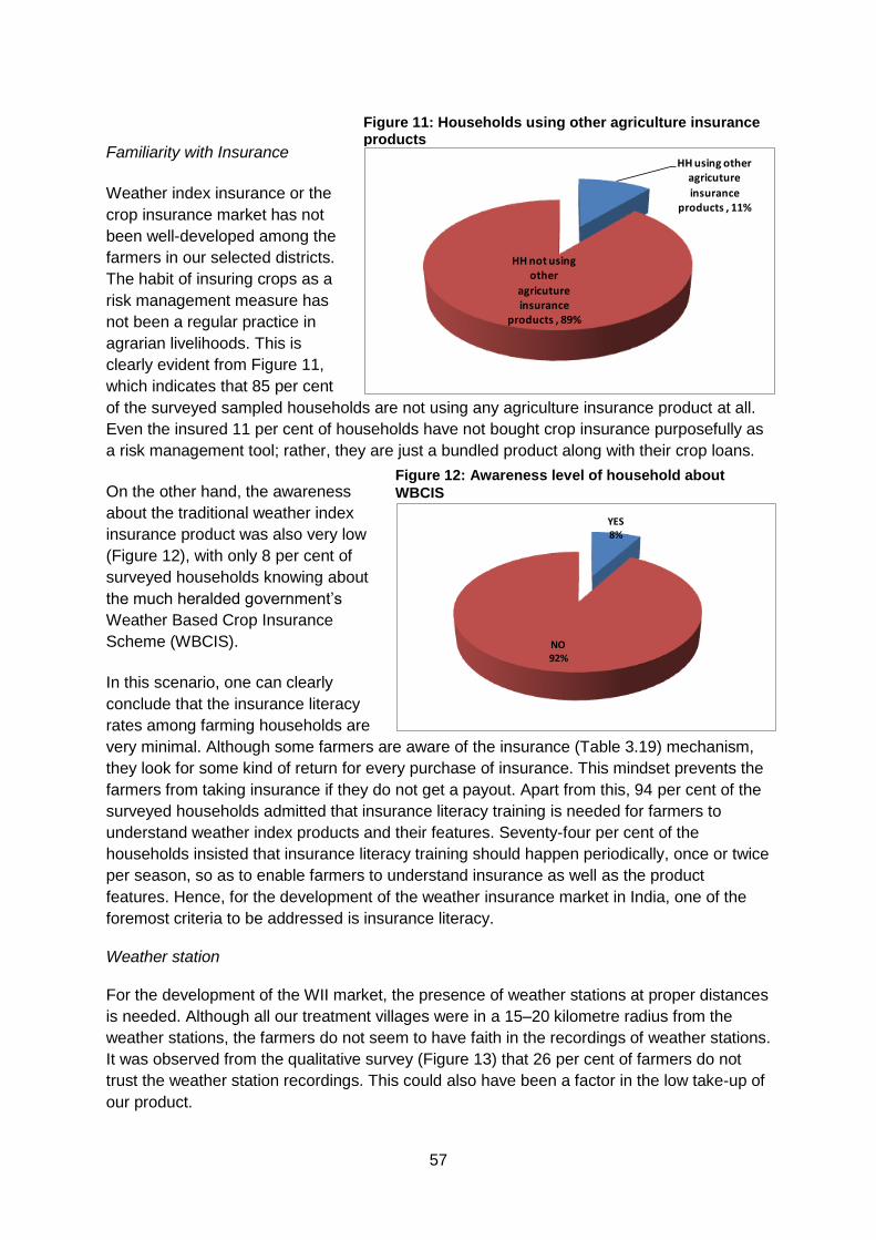
57

Familiarity with Insurance

Weather index insurance or the

crop insurance market has not

been well-developed among the

farmers in our selected districts.

The habit of insuring crops as a

risk management measure has

not been a regular practice in

agrarian livelihoods. This is

clearly evident from Figure 11,

which indicates that 85 per cent

of the surveyed sampled households are not using any agriculture insurance product at all.

Even the insured 11 per cent of households have not bought crop insurance purposefully as

a risk management tool; rather, they are just a bundled product along with their crop loans.

On the other hand, the awareness

about the traditional weather index

insurance product was also very low

(Figure 12), with only 8 per cent of

surveyed households knowing about

the much heralded government’s

Weather Based Crop Insurance

Scheme (WBCIS).

In this scenario, one can clearly

conclude that the insurance literacy

rates among farming households are

very minimal. Although some farmers are aware of the insurance (Table 3.19) mechanism,

they look for some kind of return for every purchase of insurance. This mindset prevents the

farmers from taking insurance if they do not get a payout. Apart from this, 94 per cent of the

surveyed households admitted that insurance literacy training is needed for farmers to

understand weather index products and their features. Seventy-four per cent of the

households insisted that insurance literacy training should happen periodically, once or twice

per season, so as to enable farmers to understand insurance as well as the product

features. Hence, for the development of the weather insurance market in India, one of the

foremost criteria to be addressed is insurance literacy.

Weather station

For the development of the WII market, the presence of weather stations at proper distances

is needed. Although all our treatment villages were in a 15–20 kilometre radius from the

weather stations, the farmers do not seem to have faith in the recordings of weather stations.

It was observed from the qualitative survey (Figure 13) that 26 per cent of farmers do not

trust the weather station recordings. This could also have been a factor in the low take-up of

our product.

YES8%

NO92%

Figure 11: Households using other agriculture insurance products

Figure 12: Awareness level of household about

WBCIS

HH using other agricuture

insurance products , 11%

HH not using other

agricuture insurance

products , 89%

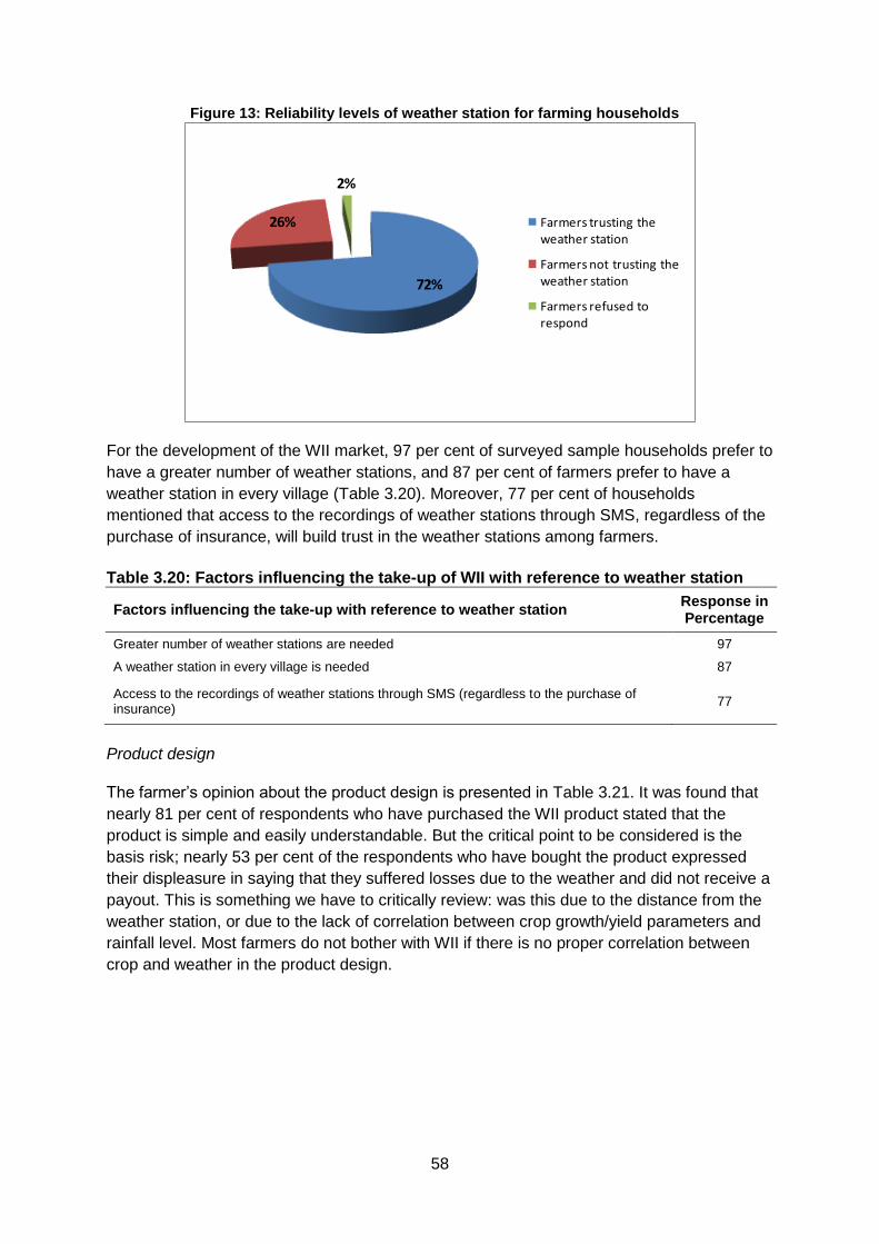
58

Figure 13: Reliability levels of weather station for farming households

For the development of the WII market, 97 per cent of surveyed sample households prefer to

have a greater number of weather stations, and 87 per cent of farmers prefer to have a

weather station in every village (Table 3.20). Moreover, 77 per cent of households

mentioned that access to the recordings of weather stations through SMS, regardless of the

purchase of insurance, will build trust in the weather stations among farmers.

Table 3.20: Factors influencing the take-up of WII with reference to weather station

Factors influencing the take-up with reference to weather station Response in Percentage

Greater number of weather stations are needed 97

A weather station in every village is needed 87

Access to the recordings of weather stations through SMS (regardless to the purchase of insurance)

77

Product design

The farmer’s opinion about the product design is presented in Table 3.21. It was found that

nearly 81 per cent of respondents who have purchased the WII product stated that the

product is simple and easily understandable. But the critical point to be considered is the

basis risk; nearly 53 per cent of the respondents who have bought the product expressed

their displeasure in saying that they suffered losses due to the weather and did not receive a

payout. This is something we have to critically review: was this due to the distance from the

weather station, or due to the lack of correlation between crop growth/yield parameters and

rainfall level. Most farmers do not bother with WII if there is no proper correlation between

crop and weather in the product design.

72%

26%

2%

Farmers trusting the weather station

Farmers not trusting the weather station

Farmers refused to respond

59

Table 3.21: Farmers’ opinion about the WII product design

Farmers’ opinion about the product Response in Percentage

Easily understandable product / simple product 81

Useful product 69

Covered all the expected weather risks 65

Experienced basis risk (suffered loss due to weather, but did not get a payout ) 53

On the other hand, through our FGDs we found that the farmers are expecting more risks to

be covered by a simple WII product like this one. This is also evident from Table 3.21, where

only 65 per cent of the respondents reported that the product covered all the expected

weather risks. This was mainly because of the lack of understanding about the weather

index insurance product.

Similarly, most farmers expressed the view that the payout level was very minimal, which

deterred many farmers from purchasing the insurance. Figure 14 projects the farmer’s view

about the payout level.

Only 11 per cent of the respondents opted for a realistic actual payout for one insurance

product of ₹3,000 to 4,000. A product of minimal cost (premium of ₹200 to 300) with huge

returns (payouts of ₹10,000 to ₹20,000) would definitely enhance take-up, but is of course

commercially unviable without large amounts of subsidies. These results perhaps point to a

failure in the training provided to farmers. As explained above, one of the key characteristics

in the design of the specific insurance products offered is to target heterogeneous farmers

by serving as a sort of building block towards a portfolio of insurance policies. Thus, farmers

expecting higher payouts, given unfavourable weather events, would have the possibility of

purchasing a greater number of insurance policies to cover any desired amount (within

certain limits imposed by the insurance company). Farmers expecting a payout for their total

operational costs by purchasing only one insurance policy are then showing a lack of

comprehensive understanding of the characteristics of the insurance product being offered

0

5

10

15

20

25

30

35

40

45

Rs.3000 to Rs.4000

Rs.5000 to Rs.10000

Rs.10001 to Rs.15000

Rs.20000 Refused to respond

Response in percentage

Figure 14: Farmers’ expectations for the product’s payout

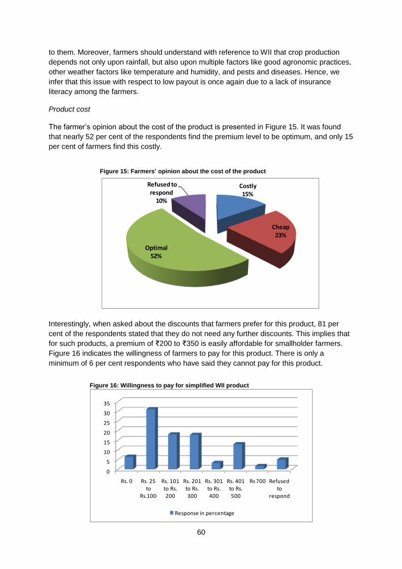
60

to them. Moreover, farmers should understand with reference to WII that crop production

depends not only upon rainfall, but also upon multiple factors like good agronomic practices,

other weather factors like temperature and humidity, and pests and diseases. Hence, we

infer that this issue with respect to low payout is once again due to a lack of insurance

literacy among the farmers.

Product cost

The farmer’s opinion about the cost of the product is presented in Figure 15. It was found

that nearly 52 per cent of the respondents find the premium level to be optimum, and only 15

per cent of farmers find this costly.

Interestingly, when asked about the discounts that farmers prefer for this product, 81 per

cent of the respondents stated that they do not need any further discounts. This implies that

for such products, a premium of ₹200 to ₹350 is easily affordable for smallholder farmers.

Figure 16 indicates the willingness of farmers to pay for this product. There is only a

minimum of 6 per cent respondents who have said they cannot pay for this product.

Costly15%

Cheap23%

Optimal52%

Refused to respond

10%

0

5

10

15

20

25

30

35

Rs. 0 Rs. 25 to

Rs.100

Rs. 101 to Rs. 200

Rs. 201 to Rs. 300

Rs. 301 to Rs. 400

Rs. 401 to Rs. 500

Rs 700 Refused to

respond

Response in percentage

Figure 16: Willingness to pay for simplified WII product

Figure 15: Farmers’ opinion about the cost of the product

61

Trust in the insurer

The level of farmers’ trust in the insurance company (HDFC ERGO) is presented in Table

3.22. It was found that 40 per cent of farmers who bought the WII and 30 per cent of farmers

who did not have trust in the insurance company. Another interesting observation that one

could infer from this is that, although trust influences take-up, trust alone is not a major

deciding factor in insurance take-up. It is clearly evident that 70 per cent of the respondents

in the no purchase group trusted the insurer, and 40 per cent of the respondents in the

purchase group did not trust the insurer. Moreover, one should also consider that private

insurance companies have started operating in India only recently, and they are just over 10

years old. Hence, it may take people some time to understand the credibility of private

insurers. If private insurers can gain the confidence of people in the case of motor insurance

or health insurance, then they can also fare well with farmers/WII insurance.

Table 3.22: Farmers’ trust in the insurer

Farmers who bought WII Farmers who did not buy WII

Trust the insurer 60% 70%

Do not trust the insurer 40% 30%

On the other hand, the reasons for not trusting the insurer are presented in Table 3.23. One

of the important reasons that require attention is that the insurer should have a good

permanent local presence in the area where the product is sold. At the moment, the product

is being sold by contractual agents who seldom visit the field after marketing. This was

stated by 29 per cent of the farmers who have bought the product, and 75 per cent of

farmers who have not bought the product. The insurers can overcome this by joining with

partners such as companies involved in contract farming or agricultural input supply, or with

community-based organisations in order to take advantage of their existing links with farmers

to market WII effectively.

Table 3.23: Reasons for not trusting the insurer

Reason for not trusting the insurer Farmers

who bought WII

Farmers who did not buy

WII

Did not get the payout 62% 0%

The insurance company people visit us only once for marketing, and after that they vanish. Insurance company doesn’t have a local office, permanent staff or contact address to share our grievances or ask our doubts

29% 75%

HDFC ERGO is a new and private company (will trust only government insurance company)

10% 25%

Peer experience

It was found during the qualitative assessment that almost all the take-ups have happened

because of peer influence among the farmers in the village. Most of the take-ups have been

among relatives, friends and people of the same caste. If one farmer has a good

understanding of the product, his presence influences others in the neighbourhood to adopt

62

the new product. However, the insurance literacy levels of these farmers taking up the

insurance product because of peer influence continues to be very low.

6.4.2 Influence of WII on the production and consumption behaviour of farmers

The impact of WII on production behaviours of farmers is presented in Table 3.24. It was

found that the impact of purchasing the WII product in 2011 or 2012, or both, was quite low.

Thirty-two per cent of the sampled surveyed farmers who have purchased WII said that WII

influenced them to purchase a higher quality or hybrid seeds, 11 per cent said that they

cultivated a larger area, 23 per cent said that they cultivated new or high-value crops, 17 per

cent said they saw some improvement in their yield or income through the adoption of

improved cultivation practices, and 3 per cent said that WII influenced them in getting

additional loans.

Table 3.24: Impact of WII on production behaviours of farmers

Impact of WII Response of farmers

who bought WII

Used hybrid seeds or high-yielding varieties because of WII 32%

Increased the area of cultivation because of WII 11%

Cultivated new crops or high-value crops because of WII 23%

Adopted improved cultivation practices because of WII 17%

Got additional loan because of WII 3%

On the other hand, although the responses were favourable in assessing the impact of the

product, it remains inconclusive on further qualitative probing. It seems that most of these

farmers had already planned to try using hybrid seeds or new crops or improved cultivation

practices, or to increase the area of cultivation. Since they had been planning this for a long

time and the introduction of our WII product occurred recently and in an unexpected manner,

there always remains the possibility that these farmers would have tried these production

practices even without WII. Moreover, we believe that a clear impact could be assessed only

when this risk management practice (of WII) becomes a regular part of the livelihood

practices of these farmers over a period of time. There were also some positive indicators,

e.g. a farmer who had taken WII said that they have intentionally bought the product just to

add strength to their being able getting a cattle loan to buy a buffalo.

The influences of WII payout on production and consumption behaviours are presented in

Table 3.25. It was found that 28 per cent of farmers who have received the payout have

mitigated the risk in crop production and managed a normal level of consumption. Although

these figures support the impact, on the other hand a larger proportion—72 per cent—of

farmers who have also received the payout mentioned that since the payout took place two

to three months later, they had to mitigate the risk through their savings or by local lending.

63

Table 3.25: Influence of WII payout on production and consumption behaviours

Impact of WII payout Response of farmers who received payout

Risk mitigated in crop production in time with the help of payout 28%

Managed normal level of consumption because of payout 28%

Nevertheless, it has to be understood that during both the years of our piloting (kharif 2011

and 2012), farmers experienced only moderate weather risk in their crop production. From a

research perspective, we feel that the impact of the WII product could have been measured

better had farmers experienced an extreme weather shock.

Benefits of Insurance would be realised better only in the situation of extreme events:

In a normal year, Fool Singh Lodi used to harvest a yield of around 5 quintals of soya bean per acre. The average cost of cultivation for him would be around ₹5,000 per acre, and he would approximately receive an income of around ₹10,000 to ₹12,000 per acre by selling his produce at the end of a normal season. Fool Singh’s crop suffered a moderate shock during kharif 2011 and kharif 2012 due to excessive rainfall, resulting in a yield of around 4 quintals per acre with an income of ₹8,000 to 9,000 per acre. He received a payout of ₹1,000 per acre during both seasons and managed to compensate his moderate yield loss to some extent through weather index insurance. According to Fool Singh, the weather shock experienced by his crop was moderated during kharif 2011 and 2012. He feels that he could have lost his entire crop if the rainfall had been extreme, and shared that the insured farmer would experience the full benefit of WII only during such extreme situations where he would receive a maximum payout of ₹4,000 per acre to be saved from total loss. Fool Singh Lodi’s uninsured neighbouring farmers also experienced a reduction in yield during kharif 2011 and 2012 due to excessive rainfall during the vegetative phase of the crop. Since the reduction in the yield of the crop did not bring a negative cash flow, they were not able to appreciate the benefit of weather index insurance to its full extent. Moreover, crop yield is determined by complex factors like the adoption of good agronomic practices, incidence of pests and diseases, and other environmental factors like light, temperature, humidity and rainfall. We cannot authentically justify that the moderated variation in yield was a result of a moderate variation in rainfall alone. Hence, the full benefit of a WII can be appreciated only in the case of severe yield loss scenarios due to the occurrence of any extreme event.

64

7. Triangulation of the results

In this section, we triangulate the results of the product take-up analysis, midline analysis

and the endline qualitative assessment on the impacts of the three types of interventions,

namely price discounts, insurance literacy training and weather station on the demand for

WII. Apart from this, it also triangulates the study results on the impact of the simplified

weather index on the smallholder farmer’s welfare by affecting their production and

consumption behaviours.

7.1 Price discounts

It was found from the take-up analysis that higher price discounts have led to an increase in

the take-up of WII. This is in accordance with the findings of Craig et al. (2013). Cole et al.

(2013) also reported a fall in the demand for WII as price increases. Furthermore, the results

of the midline analysis revealed that the provision of price discounts increases insurance

literacy as well, which we attribute to either an incentive effect of paying more attention to

training as the offered insurance products were now more appealing, or a learning-by-doing

effect of being more likely to purchase insurance once discounts were distributed. While we

hypothesised that a higher discount might provide a higher incentive to understand the

product since it is more attainable for the households; it is also possible that there is a

disincentive for the same reason. A higher discount sometimes makes households less likely

to increase their information about the product since they will not be as negatively impacted

by purchasing a poor product as those households that have to pay the full cost. Our midline

analysis did not find any definitive evidence to support either of these claims. On the other

hand, our qualitative endline assessment showed that a premium of ₹200 to ₹350 is easily

affordable for smallholder farmers and there is no need for any further discount in the

product price.

7.2 Insurance literacy training Insurance literacy training was provided before the first season (kharif 2011), but was not

repeated during the second season (kharif 2012). There were two levels of insurance literacy

training, with 50 per cent of the sampled households given a basic level of insurance literacy,

and the other 50 per cent given intensive training. It was found that the intensive literacy

training had influenced three times the take-up when compared to the basic level of training

during kharif 2011. But during kharif 2012, there does not seem to be any clear influence of

the levels of insurance literacy provided in 2011 on the take-up of the product. This seems to

imply that the impact of the differential level of insurance literacy training provided in 2011

did not carry through to kharif 2012.

On the other hand, our midline analysis revealed that the intensive training had no effect on

the comprehension of the insurance product, or on the other attitude-related questions that

households were asked. This suggests that, to the extent that intensive training had an

impact on demand, it did not come about as a result of a sustained increase in insurance

literacy. It could be that households had forgotten what they had learned by the time of the

survey (about six months later), or it could be that the additional training served more of a

marketing purpose than providing additional knowledge about the insurance itself. This is

confirmed by our qualitative endline assessment as well, where we observed that insurance

65

literacy among farming households was very minimal. We found from our qualitative

assessment that periodic insurance literacy training needs to be imparted to all farming

households on a regular basis, so as to enable them to understand the insurance and WII

product features. Hence, for the development of a weather insurance market in India, one of

the foremost criteria to be addressed is insurance literacy.

7.3 Weather station From the take-up analysis, it was found that more than two thirds of the contracts purchased

during both cropping seasons were by households located at a distance of less than 10

kilometres from the weather station, while the take-up rates fell considerably beyond this

distance from the weather station. This indicates the significant impact of the spatial basis

risk on index insurance take-up. Mobarak and Rosenzweig (2012) also find that the demand

for a WII product decreases with increase in distance to the weather station. We found

further evidence from our midline analysis that the households located closer to the newer

weather stations were significantly more satisfied with the weather station operations.

Furthermore, households located away from the weather stations had significantly lower

comprehension of insurance payouts and timing, and less trust in the insurance/insurer.

On the other hand, from our qualitative endline assessment we found that for the

development of a WII market, a weather station is needed in every village. It was also found

that access to the recordings of weather stations through SMS, regardless of the purchase

of insurance, will build trust in the weather stations among farmers.

7.4 Impact of the simplified WII on production and consumption behaviours

Our midline analysis during kharif 2011 showed that the offer of insurance (ITT) decreased

fertiliser expenditures in soya bean crop cultivation. Furthermore, the purchase of insurance

(ATE) resulted in a higher share of non-hybrid seeds to total input costs. The other

production impacts of WII observed during kharif 2011 are:

The offer of WII decreased the likelihood of farming households taking a loan;

however, when an agricultural loan was taken, it was significantly larger.

There was a positive impact in the number of smaller loans for households that

purchased insurance. However, we do not have a fully consistent explanation of our

ITT result, which shows a negative impact on the purchase of fertiliser and farmers

taking larger loans.

Households that purchased our WII were much less likely to take out government

loans with insurance, suggesting a substitution effect.

Households that were offered insurance received significantly more total transfers,

specifically in the form of gifts and donations in September and October and after the

end of the harvest, although it is not clear to us what might explain this.

Similarly, our qualitative endline study also gave us results like WII positively influencing

farmers to use hybrid seeds or high-yielding varieties, to cultivate an increased area, to

cultivate new crops, to adopt improved cultivation practices and to get additional loans.

Although these results were in line with the findings of other relevant studies such as Lybbert

et al. (2010) and Cole et al. (2011), we found that our results were very inconclusive.

66

Through further qualitative probing, we found that most of the farmers who have tried newer

or improved practices had already planned to implement them even before they came to

know about our WII. Since they had been planning this for a long time, and the introduction

of our WII product took place in an unexpected manner through our project, there remains

some doubt as to whether these farmers would have tried these production practices even

without our WII. Moreover, we believe that a very clear impact of WII could be assessed only

if this risk management practice of using WII becomes a regular part of the livelihood

practices of these farmers over a period of time.

On the other hand, that WII payouts influence the production and consumption behaviours of

farmers remains a bit inconclusive through our qualitative study. It was found that that since

the payout was done two to three months after the occurrence of risk, in a real time situation

the farmers had to mitigate their risk through their savings or by local lending. Nevertheless,

it has to be understood that during both years of our piloting (kharif 2011 and 2012), farmers

experienced only moderate weather shocks in their crop production. From a research

perspective, we feel that the impact of the WII product could have been measured more

accurately had farmers experienced extreme weather shocks.

8. Conclusions and policy implications

8.1 Conclusion

This report presents our impact evaluation study to assess the potential of our simplified WII

in satisfying the insurance demands of smallholder farmers in India. The study was carried

out for two cropping seasons with the original intention to evaluate the impact of our WII

product on the production and consumption behaviours of smallholder farmers cultivating

rainfed soya bean crop. Unfortunately, due to the low levels of take-up faced, we were not

able to carry out this intended analysis. Nevertheless, we were able to investigate the

barriers to the take-up of WII together with the responsiveness of WII demand to a set of

interventions, namely price discounts, proximity of weather stations (a proxy for basis risk)

and the intensity of training on insurance literacy. We find the following empirical evidence,

with different levels of statistical significance.

The main findings from our empirical work are:

After controlling for a large set of socio-economic covariates, the proportion of

households purchasing insurance in Bhopal district was higher than that in Dewas or

Ujjain districts. We have anecdotal information stating that it was precisely in Bhopal

that the insurance company was able to implement a better and on-time marketing

campaign, and therefore we speculate that this is a potential explanation. In this

project, we had little control over marketing activities as it was carried out by the

insurance company and as a learning experience we recommend: (i) incorporate in

the design of similar projects some degree of control over such activities, and (ii)

collect specific information to measure marketing activities when surveying

households.

67

We find that take-up is sensitive to price variations which were randomly introduced.

We estimate a price elasticity of 0.58, which is not substantially different from the

price elasticity estimated by others in other states in India.

As expected, distance to a weather station is a relevant factor in explaining the

demand for WII. As one can expect, the location of existing weather stations is not

random, and is probably correlated with where certain types of farms are located. In

this project, we installed new weather stations to properly estimate the impact of

distance on WII take-up. Our estimates indicate that distance significantly reduces

uptake, and that each kilometre from the weather station reduces take-up by 1

percentage point.

We found that households that were offered intensive training on insurance literacy

had significantly higher insurance uptake than those that were given basic training.

Take-up among those offered intensive training was about 5 per cent higher than

among those that were offered basic training only.

All random treatments (price variation, distance to weather station, training) appeared

to have the expected effect on take-up, although the effect on the amount of

insurance purchased (or number of acres insured) is much weaker in each case. Our

results are robust to including household-level covariates.

We studied the impact of a set of household characteristics on WII take-up and found

that only a few of them showed at least some evidence of such impact. We see that

loss-averse households are more likely (at a 5 per cent significance level) to

purchase HDFC’s product and insure more of their land. Weakly significant results

seem to point towards households having previously purchased weather insurance

(before project implementation) also being more likely to buy insurance and insuring

more of their land, and households previously able to access loans to cope with the

last drought being less likely to purchase insurance, indicating perhaps that credit

and insurance are seen as substitutes.

A simple computation (using our 2011 estimates) of a measure of cost-benefit

analysis of our three exogenous interventions shows that: (i) Increasing take-up rates

by 10 percentage points by insurance literacy training (which has a short-term lasting

effect) would cost $20.80 per person; (ii) Increasing take-up rates by 10 percentage

points by reducing the distance to a weather station (and installing new stations)

would cost $13.34 per person; and (iii) that to increase take-up rates by 10

percentage points by providing discounts, $2.30 per policy is needed. Therefore,

providing discounts seems to be the most cost-effective treatment to increase index

insurance take-up.

We studied the impact of offering and purchasing insurance on the basis of trust in

the insurance company and on knowledge about the product. The offer of insurance

has a significant effect on knowledge and trust, while the purchase of insurance

increased the comprehension of only certain aspects of our knowledge indicator. To

understand better the mechanisms of these effects, we analysed the impact of each

treatment arm on trust and knowledge. Our results show that reducing the distance to

68

a weather station has a positive impact on the comprehension of insurance payouts

and timing, greater satisfaction with the weather station and greater trust in the

private insurer. Also, a higher price discount has a positive impact on our overall

insurance knowledge score. We find some evidence to support two mechanisms for

this result: (i) the provision of a voucher created greater incentives to pay more

attention during the training session; and (ii) people who received vouchers were

more likely to purchase insurance and therefore were able to learn about insurance

through this process (learning-by-doing). On the contrary, intensive training has no

significant impact on our knowledge score, satisfaction with the weather station or

trust in the private insurer.

When we analyse the impact of offering insurance and purchasing insurance on

farmers’ production decisions (among them size and proportion of land cultivated

under cash crops, fertilised, irrigated and early sowed, and value and proportion of

inputs in total expenditures), we do not find conclusive evidence of such an impact,

and a non-significant impact on decisions such as the application of fertilisers, cash

crop cultivation and hybrid seed purchases do not support the evidence of other

studies. We claim that this lack of empirical evidence is in part explained by the low

take-up and therefore the low statistical power of our estimators. Likewise, we find no

detectable impact on the likelihood of taking a loan and the size of the largest loan

across all loans.

While analysing the impact on loans, we find that the offer of insurance does not

have a detectable impact on any of the following credit measures: taking a loan, the

number of loans, and some specifics about the largest loan such as size, interest rate

and purpose. However, we do find that the purchase of insurance resulted in the

taking of more loans, although we cannot provide evidence on why this happens. In

the particular case of government loans (which are linked to government insurance),

we find some evidence that households that purchase insurance are less likely to

take out government loans with government insurance. This indicates a certain

degree of substitutability between government loans and the HDFC product, as

expected.

We also consider the impact of insurance on household transfers and other sources

of income such as wage labour. We find that only households that were offered

insurance received a significantly greater number of total transfers, specifically in the

form of gifts and donations in September, October and November, and after the end

of the harvest. We also tested whether households in villages where payouts were

made were more likely to receive transfers, but did not find anything to support this

hypothesis.

When we looked at the second season of index insurance sales, we confirmed that

price variations and distance to the weather station were also strongly associated

with purchases (especially in the subsample of villages served by new stations).

Interestingly, the effect of training seems to fade over time: although receiving

intensive training significantly increased demand in the season immediately following

training (2011), it had no significant effect on demand in 2012.

69

Also there is no evidence that the discount received in 2011 had any impact on the

2012 demand, which is somehow surprising, given that we found that households

that had received a subsidy had a much better understanding of the insurance

product. In sum, the results suggest that insurance literacy training and subsidies

have an immediate, but not sustained, effect on demand.

Finally, we found evidence that purchasing insurance in 2011 and receiving a payout

is strongly positively correlated with the decision to purchase insurance in the

subsequent season. However, observing other households in the village receiving a

payout seems to have no impact on demand.

8.2 Policy implications and recommendations:

We derive some policy implications and recommendations from this project:

During the implementation of this project, we were able to validate that weather risk

is a big source of uncertainty and concern for farmers in the districts where we have

worked. Despite the low take-up for the specific product we have tested, the majority

of farmers expressed interest in having an instrument that helps them insure against

weather and production risks. Therefore, keeping an active policy for piloting, testing

and improving micro-insurance products for small farmers is advisable.

This project’s intention was to shed light on the specific characteristics that an

insurance product should have to make farmers move from simply showing an

interest in WII to taking more concrete action and purchasing it. We proposed a new

product which we claim is simple to understand and which gives farmers a range of

options to choose from according to their own risk profile. The evidence gathered

from purchasing behaviour apparently indicates that these two features were not

appealing enough to encourage a sizeable share of farmers to purchase the product.

However, as our qualitative assessment shows, there are other factors that can

potentially explain the low take-up among farmers (among them a better marketing

strategy). The farmers’ perception was that the product offered was not complex or

difficult to comprehend. Also, we observed that the most preferred product changed

from one season to the next, validating to some extent the importance of giving

farmers a menu of product options to choose from. Therefore, we propose that

having an explicit policy in favour of simple and flexible products is more beneficial

than detrimental.

Given the low take-up of the product and the small fraction of land insured among

those who actually purchased the product, it has not been possible to provide

evidence on the impact of insurance purchase on production and consumption

decisions, and ultimately on farmers’ welfare. In fact, only a few pilot programmes

have been able to provide some of this evidence, and additional and conclusive

evidence is needed. This is important from a policy perspective because only with

conclusive evidence can those government agencies in charge of promoting

agricultural micro-insurance markets have a greater chance to permanently prioritise

the topic within the government and find the fiscal resources to implement more

aggressive and ambitious rural micro-insurance programmes. Therefore, we suggest

70

policies that promote pilot programmes and ensure high take-up rates. This will

enable us to measure the impact on farmers’ welfare. This project has contributed

additional evidence to show that demand for WII is sensitive to prices, distance to

weather stations and an understanding of the product. Hence, these three

instruments can be used, at least in subsamples of the target population, to achieve

high take-up rates in pilot programmes. And the relevant government agency (i.e. the

Ministry of Agriculture) should invest resources in these three instruments while

piloting and gathering evidence. This implies the provision of important discounts, a

dense network of weather stations in piloting regions and periodic training and

information activities.

One important learning experience from this project is to give priority to marketing

activities, which should include proper delivery channels. Most agricultural micro-

insurance pilot programmes in India and elsewhere are usually designed and led by

economists, financial experts, impact evaluators or development consultants, and

less attention is probably given to marketing experts. One lesson from this project is

that a proper marketing strategy is a key element in piloting new insurance products

and can become a crucial constraint when marketing is the weak link. This requires

bringing in marketing experts from the time the project is being designed and during

pilot implementation. Our qualitative assessments clearly show that a large

proportion of farmers have no recollection of the product offered, that some farmers

were not able to purchase the product because the insurer had no presence in their

villages, and that those who purchased the product were expecting some return, no

matter what. Marketing should perhaps be conceptualised as a permanent process

rather than as a few specific activities that take place at specific points in time; again,

marketing experts should play a large role in the project design and in formulating a

comprehensive marketing strategy.

With respect to marketing activities, it might be the case that some activities are not

cost-effective from an individual business perspective, e.g. no insurance company in

India has the required manpower or resources to reach out to all farmers in every

village repeatedly to sell WII products. Therefore, it is important to explore alternative

delivery channels for marketing WII products and exploit economies of scale. For this

purpose, it is worth considering building partnerships among insurers and other

companies, such as those involved in contract farming or agricultural input supply, or

community-based organisations or microfinance institutions in order to take

advantage of their existing links with farmers to market WII effectively. When using

local institutions, this will also enhance the farmers’ trust in the insurer.

Timely provision of weather data to the insurers is important as it enables quick

indemnification. Although theoretically WII can trigger a payout immediately at the

end of the cover period, it takes longer, as has been the case in this project. It was

found that there has been a delay of approximately two to three months on the part of

the insurance company in making the final payout to the beneficiaries. This is mainly

because of the delay in receiving the weather data officially from the weather

stations. Such a delay in indemnity settlement has a great impact when the cover

period of WII is split into smaller phases during the crop cycle. In such a situation, the

weather-affected insured farmers will expect payouts immediately after the end of the

71

cover period for taking corrective action. A delay in the settlement of indemnity will

spoil one central advantage of WII contracts, which should be exploited to make

these products more appealing to farmers. Moreover, delays in indemnity settlement

create an adverse attitude among farmers vis-à-vis purchasing WII contracts for the

subsequent phases of crop growth. On the other hand, it was also observed from our

qualitative study that access to the recordings of weather stations through SMS,

regardless of the purchase of insurance, might be considered part of a

comprehensive marketing strategy as it helps build trust in the weather stations.

Hence, institutional arrangements have to be worked out between the weather

service providers and insurers so as to reduce the delay in officially providing

weather data for WII. The Insurance Regulatory and Development Authority (IRDA)

in India should be more active in enforcing regulatory measures so as to avoid these

administrative delays.

Our project shows that an insurance literacy training intervention has a short-term

impact on demand, but with no significant impact on understanding or demand after a

year of its implementation. Hence, it is worth exploring the implementation of a

strategy in which training and insurance literacy are part of a permanent process (at

least for some initial years), rather than a one-time activity. We propose to consider

insurance literacy trainings that are imparted through existing agriculture extension

programmes in India; the incremental costs should be minimal, and the potential

medium/long-term benefits could be important (although rigorous evidence of this is

lacking and would require a longer-term research project).

Our qualitative assessment study tells us that basis risk is a real factor that farmers

take into account when showing satisfaction or dissatisfaction with a WII product. We

found that nearly 53 per cent of the respondents who have bought the product

expressed their displeasure by saying that they suffered losses due to the weather

but did not receive a payout. This is something that needs to be critically reviewed;

was this due to the distance from the weather station or due to the lack of correlation

between crop growth/yield parameters and rainfall level? The bottom line is that high

quality WII products are a precondition for a sustained demand, as in any other

industry. And in this case, a high quality product is one with no or minimal basis risk.

We know that this depends on establishing an accurate correlation between

productivity levels (yields) and weather variations, as well as with other factors.

However, one key input to come up with improved, low basis risk and affordable

products is accurate information. So far, the proportion of yield loss due to weather

indices has not been quantified by any sound agricultural study in India. Here there is

scope for an active role for the government and research institutions in the country to

improve access to all relevant (current and historical) information and conduct

rigorous studies to establish the best indices that correlate with yield loss, ultimately

leading to the design of high-quality WII products.

Affordable premiums have been proven in this and other studies to impact take-up

rates for WII products In this project in particular, by offering products with low sums

insured, most farmers have found that premiums between ₹200 and ₹350 are

affordable, although some might not have had the full understanding that comes

precisely with a low sum insured. However, outside of this project is a perception that

72

premium rates for WII are high and largely unaffordable for small farmers. This is in

part explained by insurers’ administrative costs and re-insurance costs. The latter will

probably stay or become even more costly in the scenario of climate change and

global warming. To keep premiums affordable for small-scale farmers, there is need

for the micro-insurance industry, reinsurers and the government to look jointly at cost

structures and together find alternatives to keep premiums low, rather than simply

asking the government to provide subsidies.

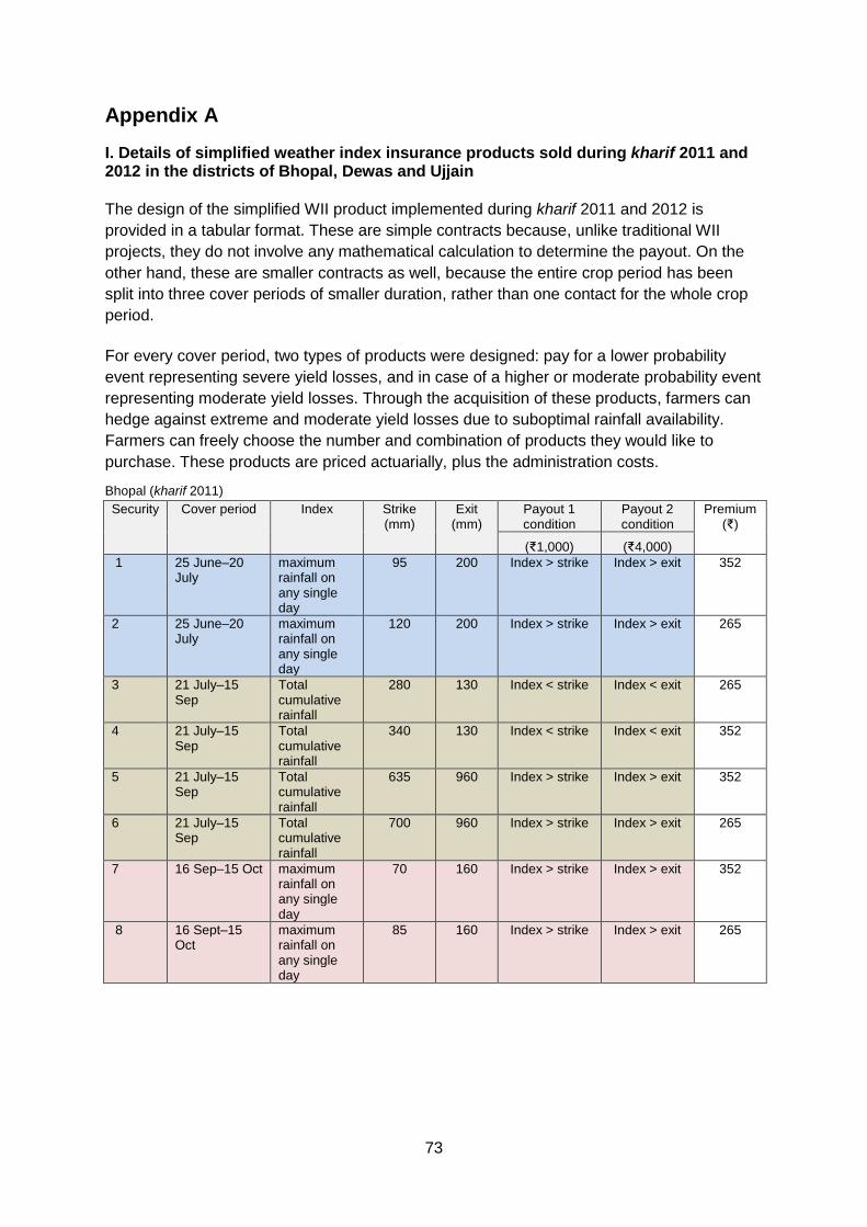
73

Appendix A

I. Details of simplified weather index insurance products sold during kharif 2011 and 2012 in the districts of Bhopal, Dewas and Ujjain

The design of the simplified WII product implemented during kharif 2011 and 2012 is

provided in a tabular format. These are simple contracts because, unlike traditional WII

projects, they do not involve any mathematical calculation to determine the payout. On the

other hand, these are smaller contracts as well, because the entire crop period has been

split into three cover periods of smaller duration, rather than one contact for the whole crop

period.

For every cover period, two types of products were designed: pay for a lower probability

event representing severe yield losses, and in case of a higher or moderate probability event

representing moderate yield losses. Through the acquisition of these products, farmers can

hedge against extreme and moderate yield losses due to suboptimal rainfall availability.

Farmers can freely choose the number and combination of products they would like to

purchase. These products are priced actuarially, plus the administration costs.

Bhopal (kharif 2011)

Security Cover period Index Strike (mm)

Exit (mm)

Payout 1 condition

Payout 2 condition

Premium (₹)

(₹1,000) (₹4,000)

1 25 June–20 July

maximum rainfall on any single day

95 200 Index > strike Index > exit 352

2 25 June–20 July

maximum rainfall on any single day

120 200 Index > strike Index > exit 265

3 21 July–15 Sep

Total cumulative rainfall

280 130 Index < strike Index < exit 265

4 21 July–15 Sep

Total cumulative rainfall

340 130 Index < strike Index < exit 352

5 21 July–15 Sep

Total cumulative rainfall

635 960 Index > strike Index > exit 352

6 21 July–15 Sep

Total cumulative rainfall

700 960 Index > strike Index > exit 265

7 16 Sep–15 Oct maximum rainfall on any single day

70 160 Index > strike Index > exit 352

8 16 Sept–15 Oct

maximum rainfall on any single day

85 160 Index > strike Index > exit 265

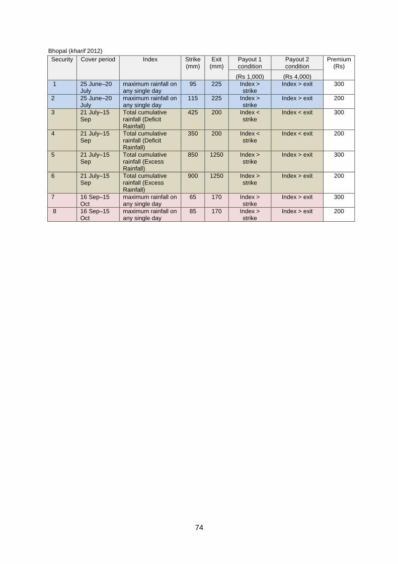
74

Bhopal (kharif 2012)

Security Cover period Index Strike (mm)

Exit (mm)

Payout 1 condition

Payout 2 condition

Premium (Rs)

(Rs 1,000) (Rs 4,000)

1 25 June–20 July

maximum rainfall on any single day

95 225 Index > strike

Index > exit 300

2 25 June–20 July

maximum rainfall on any single day

115 225 Index > strike

Index > exit 200

3 21 July–15 Sep

Total cumulative rainfall (Deficit Rainfall)

425 200 Index < strike

Index < exit 300

4 21 July–15 Sep

Total cumulative rainfall (Deficit Rainfall)

350 200 Index < strike

Index < exit 200

5 21 July–15 Sep

Total cumulative rainfall (Excess Rainfall)

850 1250 Index > strike

Index > exit 300

6 21 July–15 Sep

Total cumulative rainfall (Excess Rainfall)

900 1250 Index > strike

Index > exit 200

7 16 Sep–15 Oct

maximum rainfall on any single day

65 170 Index > strike

Index > exit 300

8 16 Sep–15 Oct

maximum rainfall on any single day

85 170 Index > strike

Index > exit 200

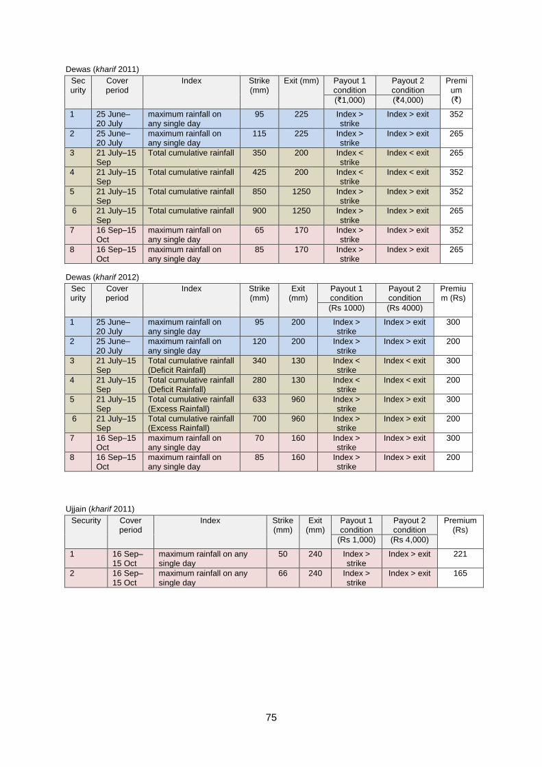
75

Dewas (kharif 2011)

Security

Cover period

Index Strike (mm)

Exit (mm) Payout 1 condition

Payout 2 condition

Premium (₹) (₹1,000) (₹4,000)

1 25 June–20 July

maximum rainfall on any single day

95 225 Index > strike

Index > exit 352

2 25 June–20 July

maximum rainfall on any single day

115 225 Index > strike

Index > exit 265

3 21 July–15 Sep

Total cumulative rainfall 350 200 Index < strike

Index < exit 265

4 21 July–15 Sep

Total cumulative rainfall 425 200 Index < strike

Index < exit 352

5 21 July–15 Sep

Total cumulative rainfall 850 1250 Index > strike

Index > exit 352

6 21 July–15 Sep

Total cumulative rainfall 900 1250 Index > strike

Index > exit 265

7 16 Sep–15 Oct

maximum rainfall on any single day

65 170 Index > strike

Index > exit 352

8 16 Sep–15 Oct

maximum rainfall on any single day

85 170 Index > strike

Index > exit 265

Dewas (kharif 2012)

Security

Cover period

Index Strike (mm)

Exit (mm)

Payout 1 condition

Payout 2 condition

Premium (Rs)

(Rs 1000) (Rs 4000)

1 25 June–20 July

maximum rainfall on any single day

95 200 Index > strike

Index > exit 300

2 25 June–20 July

maximum rainfall on any single day

120 200 Index > strike

Index > exit 200

3 21 July–15 Sep

Total cumulative rainfall (Deficit Rainfall)

340 130 Index < strike

Index < exit 300

4 21 July–15 Sep

Total cumulative rainfall (Deficit Rainfall)

280 130 Index < strike

Index < exit 200

5 21 July–15 Sep

Total cumulative rainfall (Excess Rainfall)

633 960 Index > strike

Index > exit 300

6 21 July–15 Sep

Total cumulative rainfall (Excess Rainfall)

700 960 Index > strike

Index > exit 200

7 16 Sep–15 Oct

maximum rainfall on any single day

70 160 Index > strike

Index > exit 300

8 16 Sep–15 Oct

maximum rainfall on any single day

85 160 Index > strike

Index > exit 200

Ujjain (kharif 2011)

Security Cover period

Index Strike (mm)

Exit (mm)

Payout 1 condition

Payout 2 condition

Premium (Rs)

(Rs 1,000) (Rs 4,000)

1 16 Sep–15 Oct

maximum rainfall on any single day

50 240 Index > strike

Index > exit 221

2 16 Sep– 15 Oct

maximum rainfall on any single day

66 240 Index > strike

Index > exit 165

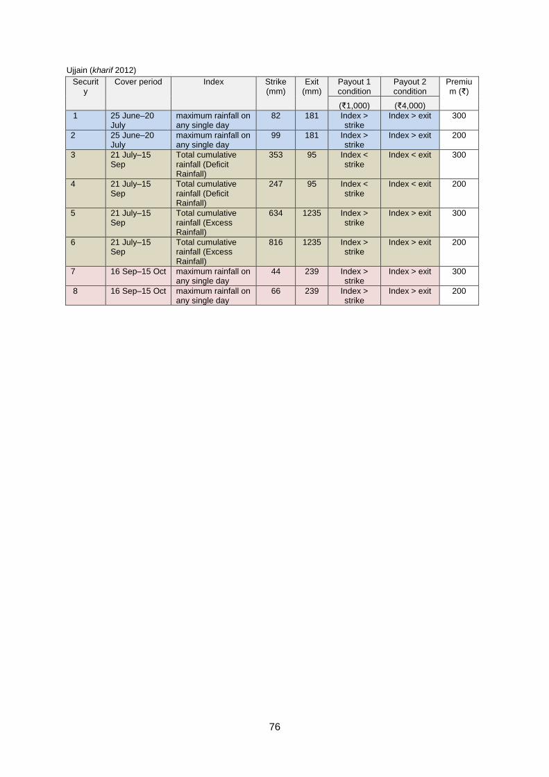
76

Ujjain (kharif 2012)

Security

Cover period Index Strike (mm)

Exit (mm)

Payout 1 condition

Payout 2 condition

Premium (₹)

(₹1,000) (₹4,000)

1 25 June–20 July

maximum rainfall on any single day

82 181 Index > strike

Index > exit 300

2 25 June–20 July

maximum rainfall on any single day

99 181 Index > strike

Index > exit 200

3 21 July–15 Sep

Total cumulative rainfall (Deficit Rainfall)

353 95 Index < strike

Index < exit 300

4 21 July–15 Sep

Total cumulative rainfall (Deficit Rainfall)

247 95 Index < strike

Index < exit 200

5 21 July–15 Sep

Total cumulative rainfall (Excess Rainfall)

634 1235 Index > strike

Index > exit 300

6 21 July–15 Sep

Total cumulative rainfall (Excess Rainfall)

816 1235 Index > strike

Index > exit 200

7 16 Sep–15 Oct maximum rainfall on any single day

44 239 Index > strike

Index > exit 300

8 16 Sep–15 Oct maximum rainfall on any single day

66 239 Index > strike

Index > exit 200

77

References Adesina, AA and J Baidu-Forson. 1995. Farmers’ perceptions and adoption of new

agricultural technology: evidence from analysis in Burkina Faso and Guinea, West Africa.

Agricultural Economics, 13(1), pp.1-9.

Bryan, G, 2010. Ambiguity and insurance, Mimeo. New Haven, CT: Yale University.

Badatya, KC, 2005. Managing of drought in Indian agriculture: role of credit institutions.

Agricultural Economics Research Review, 18, pp.19-34.

Cai, de Janvry and Sadoulet. 2013. Social networks and the decision to insure. Available at https://bepp.wharton.upenn.edu/bepp/assets/File/AE-S13-Cai.pdf

Clarke, DJ, 2010. A theory of rational hedging, Mimeo. Oxford: University of Oxford.

Clarke, DJ, 2011. A theory of rational demand for index insurance, Economics Series

Working Papers 572, Oxford: University of Oxford.

Clarke, D and Kalani, G, 2011. Microinsurance decisions: evidence from Ethiopia. Oxford:

University of Oxford.

Cole, S, Gine, X and Vickery, J, 2011. How does risk management influence production

decisions? Evidence from a field experiment, Working Paper. Northeast Universities

Development Consortium Conference 2011.

Cole, S, Giné, X, Tobacman, J, Townsend, RM, Topalova, PB and Vickery, VI, 2012.

Barriers to household risk management: evidence from India. SSRN Scholarly Paper ID

1374076. Rochester, NY: Social Science Research Network. Available at

http://papers.ssrn.com/abstract=1374076.

Cole, S, Giné, X, Tobacman, J, Topalova, PB, Townsend, RM and Vickery, JI, 2013. Barriers

to household risk management: evidence from India. American Economic Journal: Applied

Economics, 5(1), pp.104-35.

Cole, S, Stein, D and Tobacman, J, 2014. Dynamics of demand for index insurance: evidence from a long-run field experiment. American Economic Review, 104(5), pp. 284-90.

Ellis, F, 2000. Rural livelihoods and diversity in developing countries. Oxford: Oxford

University Press.

Fafchamps, M and Pender, J, 1997. Precautionary saving, credit constraints, and irreversible

investment: theory and evidence from semiarid India. Journal of Business and Economic

Statistics,15(2), pp.180-94.

Feder, G, Just, RE and Zilberman, D, 1985. Adoption of agricultural innovations in

developing countries: a survey. Economic Development and Cultural Change, 33(2), pp.

255-98.

78

Feder, G and O’Mara, G, 1982. On information and innovation diffusion: a Bayesian

approach. American Journal of Agricultural Economics, vol. 64, pp.141-45.

Gautam, MP, Hazell, P and Alderman, H, 1994. Rural demand for drought insurance. Policy

Research Working Paper No. 1383. Washington, DC: World Bank.

Gine, X, Townsend, R and Vickery, J, 2007. Statistical analysis of rainfall insurance payouts in southern India, American Journal of Agricultural Economics, vol. 89(5), pp. 1248-1254.

Gine, X, Townsend, R and Vickery, J, 2008. Patterns of rainfall insurance participation in

rural India. The World Bank Economic Review. Available at

http://siteresources.worldbank.org/DEC/Resources/Patterns_of_Rainfall_Insurance_India_S

ep_09.pdf.

Government of India (GOI), 2007. Report of the working group on risk management in

agriculture for the eleventh five year plan (2007-12). New Delhi: Planning Commission,

Government of India.

Hill, RV, Hoddinott, J and Kumar, N, 2011. Adoption of weather index insurance: learning

from willingness to pay among a panel of households in rural Ethiopia. International Food

Policy Research Institute Discussion Paper.

International Fund for Agriculture Development (IFAD) and World Food Programme (WFP),

2010. The potential for scale and sustainability in weather index insurance for agriculture

and rural livelihoods. Available at

http://documents.wfp.org/stellent/groups/public/documents/communications/wfp220176.pdf.

Karlan, D, Osei, R, Osei-Akoto, I, Udry, C, 2012. Agricultural decisions after relaxing credit and risk constraints, Working Paper, New Haven, CT: Yale University.

Karlan, D, Osei, R, Osei-Akoto, I, Udry, C, 2014. Agricultural decisions after relaxing credit and risk constraints. The Quarterly Journal of Economics, vol.129(2), pp.597-652

Lybbert, T, Galarza, FB, McPeak, J, Barrett, C, Boucher, SR, Carter, MR, Chantarat, S,

2010. Dynamic field experiments in development economics: risk valuation in Morocco,

Kenya and Peru. Paper presented at the I4 Scientific Meeting, Rome, 15-16 January.

McIntosh, C, Sarris, A and Papadopoulos, F, 2013. Productivity, credit, risk, and the demand

for weather index insurance in smallholder agriculture in Ethiopia. Agricultural Economics,

vol.44, pp.399-417.

McKenzie, D, 2011. Beyond baseline and follow-up: the case of more T in experiments.

Policy Research Working Paper No. 5639. Washington, DC: World Bank.

Mobarak, AM and Rosenzweig, M, 2012. Selling formal insurance to the informally insured.

Working Paper No. 97, Economic Growth Center Discussion Paper No. 1007. New Haven,

CT: Department of Economics, Yale University.

Morduch, J, 1991. Risk and welfare in developing countries. PhD Thesis. New Haven, CT:

Harvard University.

79

Nair, R, 2010. Crop insurance in India: changes and challenges. Economic and Political

Weekly, XLV(6).

O'Mara, GT, 1971. A decision theoretic view of the microeconomics of technique diffusion. Ph.D. thesis, Stanford University.

O’Mara, G, 1980. The Micro-economics of technique adoption by small-holding Mexican

farmers. Washington, DC: World Bank Development Research Center.

Rosenzweig, M and Binswanger, H, 1993. Wealth, weather risk and the composition and

profitability of agricultural investments. Economic Journal, 103, pp.56-78.

Schultz, TW, 1981. Investing in people: the economics of population quality. Berkeley and

Los Angeles, CA: University of California Press.

Singh, G, 2010. Crop insurance in India, IIM Ahmedabad, Research and Publications, W.P.

No. 2010-06-01. Available at http://www.iimahd.ernet.in/publications/data/2010-06-

01Singh.pdf.

Stein, D, 2011. Paying premium with the insurer’s money: How loss aversion drives

insurance decisions in a repeated interaction. Unpublished. cited from: Cole, S, Stein, D and

Tobacman, J. 2014. Dynamics of demand for index insurance: evidence from a long-run field

experiment. American Economic Review, vol.104(5), pp. 284-90.

World Bank and GFDRR, 2011. Enhancing crop insurance in India, Report no. 61491-IN.

Available at

http://openknowledge.worldbank.org/bitstream/handle/10986/2748/614910ESW0P1081Tech

nical0Report1FIN.pdf?sequence=1.

80

Publications in the 3ie Impact Evaluation Report Series

The following reports are available from http://www.3ieimpact.org/en/publications/3ie-impact-evaluation-reports/3ie-impact-evaluations/

The promise of preschool in Africa: A randomised impact evaluation of early childhood

development in rural Mozambique, 3ie Impact Evaluation Report 1. Martinez, S, Naudeau, S

and Pereira, V (2012)

A rapid assessment randomised-controlled trial of improved cookstoves in rural Ghana, 3ie

Impact Evaluation Report 2. Burwen, J and Levine, DI (2012)

The GoBifo project evaluation report: Assessing the impacts of community-driven

development in Sierra Leone, 3ie Impact Evaluation Report 3. Casey, K, Glennerster, R and

Miguel, E (2013)

Does marginal cost pricing of electricity affect groundwater pumping behaviour of farmers?

Evidence from India, 3ie Impact Evaluation Report 4. Meenakshi, JV, Banerji, A, Mukherji, A

and Gupta, A (2013)

Impact evaluation of the non-contributory social pension programme 70 y más in Mexico, 3ie

Impact Evaluation Report 5. Rodríguez, A, Espinoza, B, Tamayo, K, Pereda, P, Góngora, V,

Tagliaferro, G and Solís, M (2014)

The impact of daycare on maternal labour supply and child development in Mexico, 3ie

Impact Evaluation Report 6. Angeles, G, Gadsden, P, Galiani, S, Gertler, P, Herrera, A,

Kariger, P and Seira, E (2014)

Social and economic impacts of Tuungane: final report on the effects of a community-driven

reconstruction programme in the Democratic Republic of Congo, 3ie Impact Evaluation

Report 7. Humphreys, M, Sanchez de la Sierra, R and van der Windt, P (2013)

Paying for performance in China’s battle against anaemia, 3ie Impact Evaluation Report 8.

Zhang, L, Rozelle, S and Shi, Y (2013)

No margin, no mission? Evaluating the role of incentives in the distribution of public goods in

Zambia, 3ie Impact Evaluation Report 9. Ashraf, N, Bandiera, O and Jack, K (2013)

Truth-telling by third-party audits and the response of polluting firms: Experimental evidence

from India, 3ie Impact Evaluation Report 10. Duflo, E, Greenstone, M, Pande, R and Ryan,

N (2013)

An impact evaluation of information disclosure on elected representatives’ performance:

evidence from rural and urban India, 3ie Impact Evaluation Report 11. Banerjee, A, Duflo, E,

Imbert, C, Pande, R, Walton, M and Mahapatra, B (2014)

Targeting the poor: evidence from a field experiment in Indonesia, 3ie Impact Evaluation

Report 12. Atlas, V, Banerjee, A, Hanna, R, Olken, B, Wai-poi, M and Purnamasari, R (2014)

81

Scaling up male circumcision service provision: results from a randomised evaluation in

Malawi, 3ie Impact Evaluation Report 13. Thornton, R, Chinkhumba, J, Godlonton, S and

Pierotti, R (2014)

Providing collateral and improving product market access for smallholder farmers: a

randomised evaluation of inventory credit in Sierra Leone, 3ie Impact Evaluation Report 14.

Casaburi, L, Glennerster, R, Suri, T and Kamara, S (2014)

A youth wage subsidy experiment for South Africa, 3ie Impact Evaluation Report 15.

Levinsohn, J, Rankin, N, Roberts, G and Schöer, V (2014)

The impact of mother literacy and participation programmes on child learning: evidence from

a randomised evaluation in India, 3ie Impact Evaluation Report 16. Banerji, R, Berry, J and

Shortland, M (2014)

Assessing long-term impacts of conditional cash transfers on children and young adults in

rural Nicaragua, 3ie Impact Evaluation Report 17. Barham, T, Macours, K, Maluccio, JA,

Regalia, F, Aguilera, V and Moncada, ME (2014)

Impact of malaria control and enhanced literacy instruction on educational outcomes among

school children in Kenya: a multi-sectoral, prospective, randomised evaluation, 3ie Impact

Evaluation Report 18. Brooker, S and Halliday, K (2015)

A randomised evaluation of the effects of an agricultural insurance programme on rural

households’ behaviour: evidence from China, 3ie Impact Evaluation Report 19. Cai, J, de

Janvry, A and Sadoulet, E (2014)

Environmental and socioeconomic impacts of Mexico's payments for ecosystem services

programme, 3ie Impact Evaluation Report 20. Alix-Garcia, J, Aronson, G, Radeloff, V,

Ramirez-Reyes, C, Shapiro, E, Sims, K and Yañez-Pagans, P (2015)

Shelter from the storm: upgrading housing infrastructure in Latin American slums, 3ie Impact

Evaluation Report 21. Galiani, S, Gertler, P, Cooper, R, Martinez, S, Ross, A and

Undurraga, R (2015)

Assessing the impact of farmer field schools on fertilizer use in China, 3ie Impact Evaluation

Report 25. Burger, N, Fu, M, Gu, K, Jia, X, Kumar, KB and Mingliang, G (2015)

A wide angle view of learning: evaluation of the CCE and LEP programmes in Haryana, 3ie

Impact Evaluation Report 22. Duflo, E, Berry, J, Mukerji, S and Shotland, M (2015)

Enhancing food production and food security through improved inputs: an evaluation of

Tanzania’s National Agricultural Input Voucher Scheme with a focus on gender impacts, 3ie

Impact Evaluation Report 23. Gine, X, Patel, S, Cuellar-Martinez, C, McCoy, S and Lauren,

R (2015)

Assessing the impact of farmer field schools on fertilizer use in China, 3ie Impact Evaluation

Report 25. Burger, N, Fu, M, Gu, K, Jia, X, Kumar, KB and Mingliang, G (2015)

Validation of hearing screening procedures in Ecuadorian schools, 3ie Impact Evaluation Report 26. Muñoz, K, White, K, Callow-Heusser, C and Ortiz, E (2015)

Impact Evaluation Series

International Initiative for Impact Evaluation 202-203, Rectangle One D-4, Saket District Centre New Delhi – 110017 India

3ie@3ieimpact.org Tel: +91 11 4989 4444

Weather index insurance (WII) has had low demand and uptake among farmers despite a recent surge in interest among private companies and policymakers. One of the reasons for the low demand is the complexity of insurance schemes. This study evaluated the impact of a simple, transparent and flexible WII product among smallholder farmers cultivating rain-fed soybean crop in the state of Madhya Pradesh in India.

The study found that the overall demand for the simplified weather index insurance products was low. In fact, there was a fall in demand as price and distance to the weather station increased. Interestingly, intensive insurance literacy training sessions conducted in the first year seemed to have no significant impact on the understanding or demand during the second year.

While purchasing insurance did not have a substantial impact, receiving a payout had a positive impact on the decision to purchase insurance in the subsequent season. However, there was no impact on demand of observing other households in the village receiving payouts. This could also be explained by low levels of trust in the product or the insurance company.

www.3ieimpact.org