“small-scale dynamo: numerics vs. analytics“€¦ · “small-scale dynamo” 1. basics 1.1...
TRANSCRIPT

“Small-Scale Dynamo: Numerics vs. Analytics“
Jennifer Schober (Institut für Theoretische Astrophysik, Heidelberg)
Collaborators: Dominik Schleicher, Christoph Federrath, Ralf Klessen, Robi Banerjee, Simon Glover
Flash-Workshop

Content
1. Basics
1.1 Magnetic fields in the Universe 1.2 Small-Scale Dynamo: Stretch-Twist-Fold Model
2. Numerical Implementation in Flash
2.1 Critical Resolution 2.2 Growth Rate: Dependence on Forcing 2.3 Growth Rate: Dependence on Mach number
3. Comparison to Analytical Results
3.1 Kazantsev Theory 3.2 Critical Reynolds Number 3.3 Growth Rate
4. Conclusion
Jennifer Schober (ITA), February 2012 2/21
“Small-Scale Dynamo”
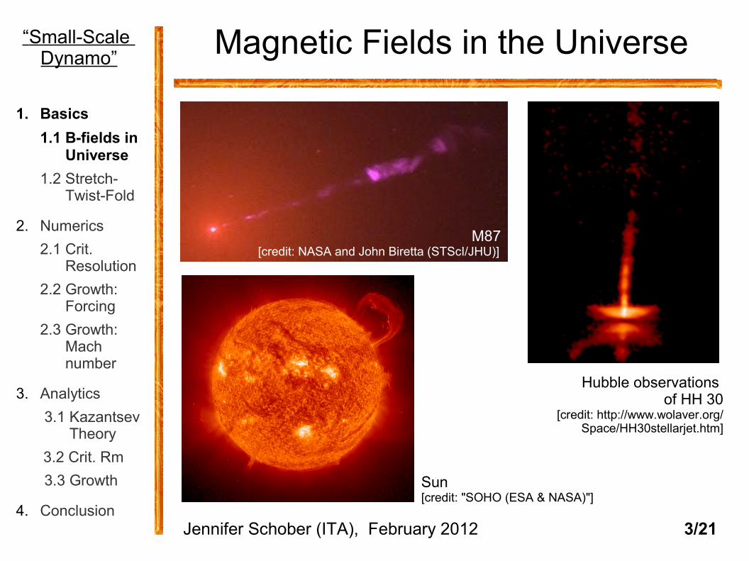
Magnetic Fields in the Universe“Small-Scale Dynamo”
Hubble observations of HH 30
[credit: http://www.wolaver.org/Space/HH30stellarjet.htm]
M87[credit: NASA and John Biretta (STScI/JHU)]
Sun[credit: "SOHO (ESA & NASA)"]
1. Basics
1.1 B-fields in Universe
1.2 Stretch- Twist-Fold
2. Numerics
2.1 Crit. Resolution
2.2 Growth: Forcing
2.3 Growth: Mach number
3. Analytics
3.1 Kazantsev Theory
3.2 Crit. Rm
3.3 Growth
4. ConclusionJennifer Schober (ITA), February 2012 3/21

Theory Observations/Upper Limits
Inflation: CMB:
QCD phase transition: reionisation:
Milky W ay:
[e.g. Turner&Widrow 1988] [e.g. Y amaz aki et al. 2006]
[e.g. Sigl et al. 1997] [e.g. Sc hleicher&Miniati 2011, in prep.]
Biermann-battery:[e.g. Xu et al. 2008] [e.g. Han. 2008]
How strong are the B-Fields?“The Small-Scale
Dynamo”
B≤4.7nG
B≤2−3nG
B≤3−4⋅103nG
B≈10−50−1nG
B≈10−3−1nG
B≈10−15 nG
=> Need mechanism that amplifies seed fields.
1. Basics
1.1 B-fields in Universe
1.2 Stretch- Twist-Fold
2. Numerics
2.1 Crit. Resolution
2.2 Growth: Forcing
2.3 Growth: Mach number
3. Analytics
3.1 Kazantsev Theory
3.2 Crit. Rm
3.3 Growth
4. ConclusionJennifer Schober (ITA), February 2012 4/21

Motivation
predicted seed B-fields << observed B-fields
=> need amplification processes small-scale dynamo
- amplifies magnetic seed field exponentially
- uses kinetic energy
from turbulence
M16[credit: NASA, ESA, STScI, J. Hester and P.
Scowen (Arizona State University)]
“Small-Scale Dynamo”
1. Basics
1.1 B-fields in Universe
1.2 Stretch- Twist-Fold
2. Numerics
2.1 Crit. Resolution
2.2 Growth: Forcing
2.3 Growth: Mach number
3. Analytics
3.1 Kazantsev Theory
3.2 Crit. Rm
3.3 Growth
4. ConclusionJennifer Schober (ITA), February 2012 5/21

Stretch-Twist-Fold Model
Source: Brandenburg&Subramanian 2005: “Astrophysical Magnetic Fields and Nonlinear Dynamo Theory“
“Small-Scale Dynamo”
1. Basics
1.1 B-fields in Universe
1.2 Stretch- Twist-Fold
2. Numerics
2.1 Crit. Resolution
2.2 Growth: Forcing
2.3 Growth: Mach number
3. Analytics
3.1 Kazantsev Theory
3.2 Crit. Rm
3.3 Growth
4. ConclusionJennifer Schober (ITA), February 2012 6/21

Numerical Results for the Small-Scale Dynamo with FLASH
“Small-Scale Dynamo”
1. Basics
1.1 B-fields in Universe
1.2 Stretch- Twist-Fold
2. Numerics
2.1 Crit. Resolution
2.2 Growth: Forcing
2.3 Growth: Mach number
3. Analytics
3.1 Kazantsev Theory
3.2 Crit. Rm
3.3 Growth
4. ConclusionJennifer Schober (ITA), February 2012 7/21

Turbulent Dynamo in FLASH
MHD in FLASH (v2.5/v4): - solution of the (non-ideal) MDH-equations - explicit viscosity and magnetic resistivity (magnetic Prandtl number )
sub- and supersonic dynamics: - 3rd order spatial reconstruction - HLL3R/HLLD Riemann solver
turbulent forcing: - forcing with stochastic Ornstein-Uhlenbeck process in momentum equation - forcing on the largest length scales => turbulence develops self-consistently on smaller scales - decomposition in solenoidal and compressive forcing possible
“Small-Scale Dynamo”
1. Basics
1.1 B-fields in Universe
1.2 Stretch- Twist-Fold
2. Numerics
2.1 Crit. Resolution
2.2 Growth: Forcing
2.3 Growth: Mach number
3. Analytics
3.1 Kazantsev Theory
3.2 Crit. Rm
3.3 Growth
4. ConclusionJennifer Schober (ITA), February 2012 8/21
Pm=/≈1

Resolution Criterion
Federrath et al., ApJ, 2011
=> small-scale dynamo works for resolution > 32 cells per Jeans length
“Small-Scale Dynamo”
1. Basics
1.1 B-fields in Universe
1.2 Stretch- Twist-Fold
2. Numerics
2.1 Crit. Resolution
2.2 Growth: Forcing
2.3 Growth: Mach number
3. Analytics
3.1 Kazantsev Theory
3.2 Crit. Rm
3.3 Growth
4. ConclusionJennifer Schober (ITA), February 2012 9/21

Different Forcing/Turbulence
Effect of different types of forcing on the structure of the field lines:
=> solenoidal forcing twists field lines more effectively
Federrath et al., PRL, 2011
“Small-Scale Dynamo”
1. Basics
1.1 B-fields in Universe
1.2 Stretch- Twist-Fold
2. Numerics
2.1 Crit. Resolution
2.2 Growth: Forcing
2.3 Growth: Mach number
3. Analytics
3.1 Kazantsev Theory
3.2 Crit. Rm
3.3 Growth
4. ConclusionJennifer Schober (ITA), February 2012 10/21

Different Forcing/Turbulence
Federrath et al., PRL, 2011
growth rate growth rate (solenodial forcing) (compressive forcing)
“Small-Scale Dynamo”
1. Basics
1.1 B-fields in Universe
1.2 Stretch- Twist-Fold
2. Numerics
2.1 Crit. Resolution
2.2 Growth: Forcing
2.3 Growth: Mach number
3. Analytics
3.1 Kazantsev Theory
3.2 Crit. Rm
3.3 Growth
4. ConclusionJennifer Schober (ITA), February 2012 11/21
=> >

Dependence on Mach Number
Federrath et al.,PRL, 2011
Emt ∝e⋅t
“Small-Scale Dynamo”
1. Basics
1.1 B-fields in Universe
1.2 Stretch- Twist-Fold
2. Numerics
2.1 Crit. Resolution
2.2 Growth: Forcing
2.3 Growth: Mach number
3. Analytics
3.1 Kazantsev Theory
3.2 Crit. Rm
3.3 Growth
4. ConclusionJennifer Schober (ITA), February 2012 12/21
( : growth rate)

Comparison to Analytical Results
“Small-Scale Dynamo”
1. Basics
1.1 B-fields in Universe
1.2 Stretch- Twist-Fold
2. Numerics
2.1 Crit. Resolution
2.2 Growth: Forcing
2.3 Growth: Mach number
3. Analytics
3.1 Kazantsev Theory
3.2 Crit. Rm
3.3 Growth
4. Conclusion Jennifer Schober (ITA), February 2012 13/21

MHD-Dynamos
idea: divide magnetic field into mean and turbulent component
put into induction equation:
=> evolution equations for mean and turbulent field (large-scale dynamo and small-scale dynamo)
B= B0 B
∂ B∂ t
=∇×v×B∇2 B
“Small-Scale Dynamo”
1. Basics
1.1 B-fields in Universe
1.2 Stretch- Twist-Fold
2. Numerics
2.1 Crit. Resolution
2.2 Growth: Forcing
2.3 Growth: Mach number
3. Analytics
3.1 Kazantsev Theory
3.2 Crit. Rm
3.3 Growth
4. Conclusion Jennifer Schober (ITA), February 2012 14/21

Kazantsev Theory
“Kazantsev Theory” [Kazantsev, 1968]: theory of the small-scale dynamo
correlation function of magnetic fluctuation:
with :
⟨ Bi x , t B j y , t ⟩=M ij r , t
M ij=ij− ri r j
r 2M N
r i r j
r2M L
∇⋅B=0
M N=12r
∂∂ r
r2M L
“Small-Scale Dynamo”
1. Basics
1.1 B-fields in Universe
1.2 Stretch- Twist-Fold
2. Numerics
2.1 Crit. Resolution
2.2 Growth:
Forcing
2.3 Growth: Mach number
3. Analytics
3.1 Kazantsev Theory
3.2 Crit. Rm
3.3 Growth
4. ConclusionJennifer Schober (ITA), February 2012 15/21

−T r ∂2r ∂2 r
U r r =−r
put magnetic correlation function into induction equation => Kazantsev equation:
“mass”
“potential”
can be solved with WKB-approximation for large magnetic Prandtl numbers ( )
U r =U ,
/
Kazantsev Theory
M L r , t ∝r e2 t
T r =T ,
“Magnetic Energy Density”
“turbulence”
“turbulence”
“Small-Scale Dynamo”
1. Basics
1.1 B-fields in Universe
1.2 Stretch- Twist-Fold
2. Numerics
2.1 Crit. Resolution
2.2 Growth:
Forcing
2.3 Growth: Mach number
3. Analytics
3.1 Kazantsev Theory
3.2 Crit. Rm
3.3 Growth
4. ConclusionJennifer Schober (ITA), February 2012 16/21

Critical Mag. Reynolds Number
Reynolds number for minimal growth rate: set in Kazantsev equation and solve for ( ), [Schober et al 2012]
result (Kolmogorov turbulence):
result (Burgers turbulence):
numerical diffusivity => depends on resolution in grid code
=> higher critical Rm/resolution for higher compressibility
=0Rm Rm=VL /
Rm110
Rm2700Rm=Rm
“Small-Scale Dynamo”
1. Basics
1.1 B-fields in Universe
1.2 Stretch- Twist-Fold
2. Numerics
2.1 Crit. Resolution
2.2 Growth:
Forcing
2.3 Growth: Mach number
3. Analytics
3.1 Kazantsev Theory
3.2 Crit. Rm
3.3 Growth
4. ConclusionJennifer Schober (ITA), February 2012 17/21

growth rate for large magnetic Prandtl numbers [Schober et al. 2012]:
(with slope of the turbulent velocity spectrum )
example 1: Kolmogorov turbulence ( )
example 2: Burgers turbulence ( )
=> faster growth at lower compressibility
Growth Rate
∝Re1−/1
∝Re1 /2
∝Re1/3
v l ∝l
=1 /3
=1 /2
“Small-Scale Dynamo”
1. Basics
1.1 B-fields in Universe
1.2 Stretch- Twist-Fold
2. Numerics
2.1 Crit. Resolution
2.2 Growth:
Forcing
2.3 Growth: Mach number
3. Analytics
3.1 Kazantsev Theory
3.2 Crit. Rm
3.3 Growth
4. ConclusionJennifer Schober (ITA), February 2012 18/21

Collapse of a Primordial Halo
Schober et al., in prep.
“Small-Scale Dynamo”
1. Basics
1.1 B-fields in Universe
1.2 Stretch- Twist-Fold
2. Numerics
2.1 Crit. Resolution
2.2 Growth:
Forcing
2.3 Growth: Mach number
3. Analytics
3.1 Kazantsev Theory
3.2 Crit. Rm
3.3 Growth
4. ConclusionJennifer Schober (ITA), February 2012 19/21

Collapse of a Primordial Halo
Schober et al., in prep.
“Small-Scale Dynamo”
1. Basics
1.1 B-fields in Universe
1.2 Stretch- Twist-Fold
2. Numerics
2.1 Crit. Resolution
2.2 Growth:
Forcing
2.3 Growth: Mach number
3. Analytics
3.1 Kazantsev Theory
3.2 Crit. Rm
3.3 Growth
4. ConclusionJennifer Schober (ITA), February 2012 20/21
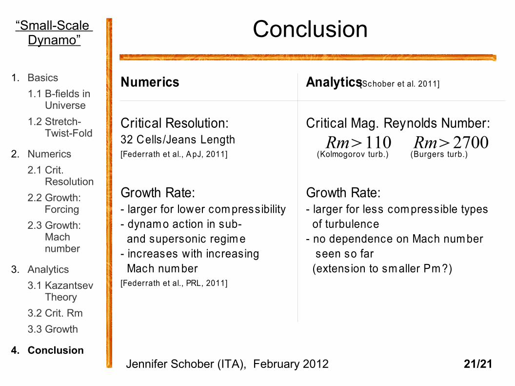
Numerics
Critical Resolution: 32 Cells/Jeans Length
Growth Rate: Growth Rate:- larger for lower com pressibility - larger for less com pressible types - dynam o action in sub- of turbulence and supersonic regim e - no dependence on Mach num ber- increases with increasing seen so far Mach num ber (extension to sm aller Pm ?)
Analytics [Schober et al. 2011]
Critical Mag. Reynolds Number:
[Federrath et al., A pJ, 2011] (Kolmogorov turb.) (Burgers turb.)
[Federrath et al., PRL, 2011]
Conclusion
Rm110 Rm2700
“Small-Scale Dynamo”
1. Basics
1.1 B-fields in Universe
1.2 Stretch- Twist-Fold
2. Numerics
2.1 Crit. Resolution
2.2 Growth:
Forcing
2.3 Growth: Mach number
3. Analytics
3.1 Kazantsev Theory
3.2 Crit. Rm
3.3 Growth
4. ConclusionJennifer Schober (ITA), February 2012 21/21

Thanks for your attention!
:-)