Submitted 7 October 2016Accepted 2 March 2017Published 28 March 2017

Corresponding authorTemesgen Hailemariam Dadi,temesgen.dadi@fu-berlin.de,temehi@gmail.com

Academic editorMauricio Rodriguez-Lanetty

Additional Information andDeclarations can be found onpage 13

DOI 10.7717/peerj.3138

Copyright2017 Dadi et al.

Distributed underCreative Commons CC-BY 4.0

OPEN ACCESS

SLIMM: species level identification ofmicroorganisms from metagenomesTemesgen Hailemariam Dadi1,2,3, Bernhard Y. Renard4, Lothar H. Wieler4,Torsten Semmler3,4 and Knut Reinert1,5

1Department of Mathematics and Computer Science, Freie Universität Berlin, Berlin, Germany2 International Max Planck Research School for Computational Biology and Scientific Computing(IMPRS-CBSC), Berlin, Germany

3Department of Veterinary Medicine, Freie Universität Berlin, Berlin, Germany4Robert Koch Institute, Berlin, Germany5Max Planck Institute for Molecular Genetics, Berlin, Germany

ABSTRACTIdentification and quantification of microorganisms is a significant step in studyingthe alpha and beta diversities within and between microbial communities respectively.Both identification and quantification of a given microbial community can be carriedout using whole genome shotgun sequences with less bias than when using 16S-rDNAsequences. However, shared regions of DNA among reference genomes and taxonomicunits pose a significant challenge in assigning reads correctly to their true origins. Theexisting microbial community profiling tools commonly deal with this problem byeither preparing signature-based unique references or assigning an ambiguous readto its least common ancestor in a taxonomic tree. The former method is limited tomaking use of the reads which can be mapped to the curated regions, while the lattersuffer from the lack of uniquelymapped reads at lower (more specific) taxonomic ranks.Moreover, even if the tools exhibited good performance in calling the organisms presentin a sample, there is still room for improvement in determining the correct relativeabundance of the organisms. We present a new method Species Level Identificationof Microorganisms from Metagenomes (SLIMM) which addresses the above issues byusing coverage information of reference genomes to remove unlikely genomes from theanalysis and subsequently gainmore uniquelymapped reads to assign at lower ranks of ataxonomic tree. SLIMM is based on a few, seemingly easy steps which when combinedcreate a tool that outperforms state-of-the-art tools in run-time and memory usagewhile being on par or better in computing quantitative and qualitative information atspecies-level.

Subjects Bioinformatics, Computational Biology, Genomics, Microbiology, TaxonomyKeywords Metagenomics, Microbial communities, Microorganisms, Taxonomic profiling, NGSdata, Microbiology

INTRODUCTIONIn the context of microbial communities, alpha diversity is the mean diversity of a singlemicrobial community and one way to represent diversity (richness) is using the number ofdifferent species in a given sample. Beta diversity on the other hand is the degree to whichthe species composition of the various microbial communities differ from another

How to cite this article Dadi et al. (2017), SLIMM: species level identification of microorganisms from metagenomes. PeerJ 5:e3138;DOI 10.7717/peerj.3138

(Whittaker, 1960). Determining the alpha and beta diversity of microbial communitiesin relevance to the host corresponding environment is ubiquitous in comparativemetagenomics. Due to this identification and quantification of microorganisms usingshotgun metagenomic reads obtained by Next Generation Sequencing (NGS) has becomea subject of growing interest in the field of microbiology. The publication of numeroustaxonomic profiling tools within the last decade only shows how appealing the subject trulyis. Lindgreen, Adair & Gardner (2016) considered 14 different sequence classification toolsbased on various approaches in a recent review of such methods.

Turning raw metagenomic reads into the relative abundance of multiple groups ofmicroorganisms (clades) residing on the sample from which the environmental DNAwas extracted and sequenced is a complicated task for several reasons. To mention a few:(1) shared (homologous) regions of genome sequences across multiple microorganismsmake an assignment of reads to their true exact difficult. (2) The range of variation in theabundance of individual groups of microbes in the sample can be high. In such cases, itis harder to detect the least abundant ones and not mistake them for noise. (3) The highdegree of variation in publicly available genome sequence lengths of different microbesmakes the quantification non-trivial (Brady & Salzberg, 2009).

In the past benchmarking of taxonomic profiling tools was done at the genus or higherlevel of the taxonomic tree. This is due to the shortcomings of many earlier tools to reportspecies-level taxonomic profiles with acceptable accuracy. However, species-level resolutionof microbial communities is desirable and more modern tools do address this (Lindgreen,Adair & Gardner, 2016; Piro, Lindner & Renard, 2016; Lindner & Renard, 2015; Francis etal., 2013). For this reason, all the benchmarks in this study were done at species-level.

In general, two distinct approaches have been widely used to tackle the challenge ofambiguous reads that originate from genomic locations shared among multiple groups oforganisms. The first approach is to prepare a signature-based database with sequences thatare unique to a clade. This method represents taxonomic clades uniquely by sequencesthat do not share common regions with other clades of the same taxonomic rank. Evenif this approach makes use of the fraction of metagenomic data from the sequencer, itcan guarantee to have only a single assignment of sequencing reads to a clade. Tools likeMetaPhlAn2 (Truong et al., 2015), GOTTCHA (Freitas et al., 2015) andmOTUs (Sunagawaet al., 2013) use this method. The second approach is based on using the full set of referencesequences available as a database and assigning ambiguous reads to their least commonancestor (LCA) in a taxonomic tree. Kraken (Wood & Salzberg, 2014), a k-mer basedread binning method, is an example of such an approach. Both approaches have certainadvantages and disadvantages. The former has an advantage in speed and precision butis limited to utilizing the reads that can be mapped uniquely to the curated regions. Thelatter approach, on the other hand, suffers from the lack of uniquely mapped reads at lower(more specific) taxonomic ranks.

Based on the final output of a method there are two categories of metagenomicclassification tools i.e., a read binning method and a taxonomic profiling method. Aread binning method assigns every single read to a node in a taxonomic tree, whereas ataxonomic profiling method tries to report which organisms or clades are present in the

Dadi et al. (2017), PeerJ, DOI 10.7717/peerj.3138 2/15

sample with or without having to assign every read to a corresponding taxon. There existsan overlap between the two categories making it possible for some read binning methodsto be used as a taxonomic profiling tool as well.

GOTTCHA uses a signature-based database specific to a given taxonomic rank, andit is highly optimized for low false discovery rate (FDR). Kraken instead uses a databasecomprising a hash table of k-mers and their corresponding node in a given taxonomictree. Then it assigns reads based on where the majority of its k-mers are located in the tree.Whenever no clear vote by the k-mers of the read exists, Kraken will assign that read to itsleast common ancestor. Kraken is a very fast read binning method, which is also often usedto do taxonomic profiling. mOTUs uses single copy universal marker genes to achieve aspecies-level abundance resolution of microbial communities. Even if the tools exhibitedgood performance in calling the organisms present in a sample, there is still room forimprovement in determining the correct relative abundance of the detected organisms.

In the following, we present a novel method called Species Level Identification ofMicroorganisms from Metagenomes (SLIMM), which addresses the limitations notedabove. During the preprocessing stage, we gather from a group of interests (e.g., Archaea,Bacteria, Viruses or any combination of these) as many reference sequences as possible anddownsize and compile taxonomic information of the gathered sequences. The taxonomicinformation is stored in the form of the SLIMM database (SLIMM_DB). We then use aread mapper to align metagenomic reads against the gathered reference sequences, whichwe consider as a preprocessing step that is often done for numerous other analyses as well(we will report the run time and memory requirement with and without preprocessing).SLIMM works on the resulting BAM/SAM alignment file. First, SLIMM uses coverageinformation both by the reads that mapped on different reference sequences and by readsuniquely mapped to a reference sequence to remove unlikely genomes from the analysissimilar to an approach taken by Lindner et al. (2013). This filtration, in turn, allows usto subsequently gain a larger number of uniquely mapped reads assigned to the reducedset of genomes which we can assign to lower ranks of a taxonomic tree. We will showthat this simple approach has indeed positive effects on the analysis. The second step isto assign the remaining non-uniquely mapped reads to the lowest common ancestor.Overall SLIMM is based on a few, seemingly easy steps resulting in a tool that outperformsstate-of-the-art tools in run-time and memory usage while being on par or better incomputing quantitative and qualitative information at the species-level which we show inthe results section. Following the recommendation in Piro, Lindner & Renard (2016) withcaution, we have carried out digital normalization on the raw reads (Brown et al., 2012)which discards low quality and redundant reads. This works by removing reads belongingto a region with high coverage depth. In our experience, the digital normalization showeda negligible improvement in calling the correct organisms.

METHODNonredundant Reference genomes databaseReference genomes from NCBI GenBank (ftp://ftp.ncbi.nlm.nih.gov/genomes/genbank/)and RefSeq (ftp://ftp.ncbi.nlm.nih.gov/genomes/refseq) archives, downloaded on

Dadi et al. (2017), PeerJ, DOI 10.7717/peerj.3138 3/15

21.05.2016, were used for the method described here. SLIMM is not limited to these publicdatabases when provided a proper mapping from sequence identifiers to a taxonomic idand a taxonomic tree that represents all the sequences in the database. For this study, weconsidered microbes under the super-kingdom of archaea and bacteria. However, one canalso easily integrate viruses into the database by using the provided SLIMM preprocessingtool. Before downloading all the genomes, we checked for redundancy by counting thenumber of available files for each species of interest. If multiple genomes were availablefor download, we then chose one in the order of (1) RefSeq (2) Complete Genome and(3) Draft Genome. This way, we received as many species as possible represented by theirbest reference genome so far available. After downloading the sequences, we checked ifevery genomic file contained only a single FASTA entry. If not, we take their concatenationseparated by a contiguous sequence of ten N’s so that reads will not accidentally map atthe joining point. The final result is a reference genome library of organisms from theinterest groups, which contains a single representative sequence per species. To cope withthe dynamically expanding reference genomes library, we implemented a feature for theSLIMM preprocessing tool that can seamlessly update the reference genome database. Inthis way, we received two databases that we named small_DB and large_DB. Small_DBcontains 2163 species with their corresponding complete genomes while large_DB contains13,192 species including those with only draft genomes available.

Read mapping against a database of interestSLIMM requires an alignment/mapping file in SAM or BAM format as an input (Fig. 1A).The alignment file can be obtained by aligning the short metagenome shotgun sequencingreads against a library of reference genomes of interest (Fig. 1B). To do so, one can usea read mapper of choice. Nevertheless, the pipeline could benefit from a faster but yetaccurate read mapper as this preprocessing step is relatively time-consuming. We make theread mapping program output secondary alignments because (1) it is very likely to havea sequencing read mapped to multiple targets, (2) a read might have multiple best hitsand (3) the best hit of a read might not be its true origin. SLIMM uses coverage landscapeinformation as shown in Fig. 1C to resolve this. We used bowtie2 (Langmead & Salzberg,2012) and Yara (Siragusa, 2013) in our preliminary experiments because they are known tobe fast read mappers with multi-threading options. Since Yara is several times faster, doesnot employ heuristics and its resulting alignments produced better profiles in some of thecases, we used it as the default mapper for this study.

Collecting coverage information of each reference genomeWe first identify which reads are mapped to which reference genomes. Then we separatethe reads uniquely assigned to a single reference sequence from those assigned to multiplereference sequences. Reads that are mapped to multiple places within a reference are alsoconsidered uniquely mapped. During this stage, SLIMM collects information like thenumber of reference genomes with mapping reads, the total number of reads and theaverage read length, which will later be used for discarding reference genomes. We thenmap reads into bins of specific width across each reference genome based on the location of

Dadi et al. (2017), PeerJ, DOI 10.7717/peerj.3138 4/15

A B

C

!✗

✗

!

""""

Figure 1 Overview of the SLIMMmethodology: (A) The SLIMM algorithm: SLIMM takes two inputs,i.e., the SLIMMDB and an alignment file in either SAM or BAM format and calculates statistical datafor each reference sequences in the database. SLIMM uses coverage information to leave out referencesequences from consideration and recalculate the statistics again. We use this, in turn, to receive readcounts that are uniquely mapped to a clade at a given taxonomic rank. (B) SLIMMPipeline: the pre-processing module of SLIMM downloads/updates all available genomes of a certain interest group(e.g., Archaea, Bacteria, Viruses or any combination of them) and tags the sequences with their corre-sponding taxonomic information. A readmapper is then used to map theWGS reads to these referencesequences. Then SLIMM algorithm uses the mapping results to produces taxonomic profile reports. (C)Reference filtering based on coverage information: an illustration of how SLIMM uses reference filter-ing based on coverage information: G2 and G3 could not pass the filtering steps because they did notcontain enough coverage by uniquely mapped reads and all reads respectively.

their mapping. The binning is done twice, once for mapped reads in general and once onlyfor uniquely mapped reads. The default width for the bins is set to the average length ofsequencing reads with an option to set it to a different value. Higher bin width means fewerbins and faster runtime, but it could lead to underrepresentation of coverage informationwhich in turn is based on whether a bin is empty or not. The bin number correspondingto a read mapped to a reference is defined by the centeral position of its mapping locationdivided by the width of the bins (integral part only). The bin number of a read mapped to

Dadi et al. (2017), PeerJ, DOI 10.7717/peerj.3138 5/15

a reference starting from locstart all the way to locend is given by:

binNumber =⌊locstart + locend

2×w

⌋(1)

where w is the width of bins a reference is partitioned into.After binning is done, coverages based on mapping reads and uniquely mapped reads

are calculated based on the corresponding bin sets. Coverage information of each referencesequence is represented by coverage percentage (%Cov) and coverage depth (CovDepth) asshown in Eqs. (2) and (3) respectively.

%Cov =|nonzeroBins||bins|

×100 (2)

CovDepth=

∑|bins|i=1

∑Nbinj=1 readLength

|bins|(3)

Where |nonzeroBins| is the number of non-zero bins, |bins| is the total number of bins inthe reference, Nbin is the number of reads in a bin and readLength is the number of basesin a read.

Discarding unlikely genomes based on coverage landscapeWe discard reference sequences with coverage percentages below a specific threshold.The threshold is calculated based on a given percentile (default 0.001) of all coveragepercentages of the genomes. In other words, after sorting the reference sequences basedon their coverage percentages in descending order we take the top N sequences that cover99.999% of the sum of all coverage percentages. This step is done for both coveragepercentage by reads that mapped on multiple references and uniquely mapped reads. Thisprocess eliminates many genomes even if they have a lot of reads mapping to them as longas they do not have a good enough coverage. Furthermore, this method was also proven toeliminate reference sequences that acquire a stack of reads only in one or two bins acrosstheir genomes which could be a result of either a sequencing artifact or a conserved regionin the genome among distant relatives.

Recalculating reads uniqueness after discarding unlikely genomesAfter discarding reference sequences, SLIMM recalculates the uniqueness of the readsagain. This recalculation can increase the number of uniquely mapped reads assignedto lower-level clades in a taxonomic tree. The recalculation of uniquely mapped reads isshown to improve the abundance estimation of a clade.

Assigning reads to their LCA and calculating abundances at a givenrankAfter recalculating the uniqueness of reads, we assign non-uniquely mapped reads totheir LCA taxon based on the NCBI taxonomic tree downloaded from ftp://ftp.ncbi.nih.gov/pub/taxonomy. Instead of using the whole NCBI taxonomic tree we use a reducedsubtree produced by the SLIMM preprocessing tool. Since we only report for a given majortaxonomic ranks namely superkingdom (domain), phylum, class, order, family, genusand species, the reduced tree contains only these taxonomic ranks. We also discarded the

Dadi et al. (2017), PeerJ, DOI 10.7717/peerj.3138 6/15

branches of the tree which are outside of the interest groups i.e., Archaea and Bacteria forthis study. This reduction saves a significant amount of computational time as assigning aread to its LCA is computationally expensive. We also propagate the number of uniquelymapped reads at a node to any of its ancestors. Then we calculate the relative abundanceof each taxonomic unit at a given rank as the uniquely mapped reads that are assigned to itdivided by the total number of uniquely mapped reads at the rank Eq. (4). We also reportan aggregated coverage depth of each clade defined as in Eq. (5).

RelABclade =Nclade

Nmapped(4)

CovDepthclade =∑Nclade

i=1 readLength∑Nchildi=1 refLength

(5)

where RelABclade is the relative abundance of a clade, Nclade is the number of reads thatare assigned to a clade, Nmapped is the total number of reads that are mapped to any clade,CovDepthclade is coverage depth of a clade, readLength is the number of bases in a read,and

∑Nchildi=1 refLength is the sum of reference lengths of children of a clade that contribute

at least one read.

RESULTS AND DISCUSSIONDatasetsFor this study, we assembled 18 different metagenomic datasets of various origins andsimulation strategies. The datasets contain (1) mock community metagenomes fromtwo different studies which were are sequenced using Illumina Genome Analyzer II(2) simulated metagenomes that resemble community profile of a real metagenomeas identified by MetaPhlAn2 (Truong et al., 2015) (3) simulation of randomly createdmicrobial communities with a varying number of organisms and range of relativeabundances. We used NeSSM (Jia et al., 2013) to do the simulations. (4) Mediumcomplexity CAMI (The Critical Assessment of Metagenome Interpretation) challengetoy datasets that are publicly available at https://data.cami-challenge.org/participate. Webelieve that this collection of datasets can represent most of the metagenomic communitiesthat a taxonomic identifier will have to handle.

We used three mock community datasets, two from the Human Microbiome Project(HMP) (HMP, 2012) containing genomes of 22 microorganisms and one from the study(Shakya et al., 2013) containing genomes of 64 microorganisms. The two datasets fromHMP are similar in the species they contain. They only differ in the abundance distribution.One contains an even abundance distribution of the microorganisms whereas the othercontains a differing abundance distribution of the 22 microorganisms.

For simulated datasets resembling an existing community we chose: (1) a metagenomeobtained from the human gut sample during theHMP (2012) (2) a freshwater metagenomedataset from Lake Lanier (Oh et al., 2011). We used MetaPhlAn2 (Truong et al., 2015)—apopular metagenomic profiling tool based on use clade-specific marker genes. Next weused the reported profile as a basis for the simulation.

Dadi et al. (2017), PeerJ, DOI 10.7717/peerj.3138 7/15

Table 1 Runtime andmemory comparison of SLIMM against existing methods.

Alignment+ SLIMM Kraken GOTTCHA mOTUs

Avg. Runtime (Seconds) 422.1+ 61.0 157.4 1727.1 1526.6Peak Memory (GB) 33.67 + 5.2 102 4 1.6

For randomly created microbiomes, we considered three communities with randomlyselected member organisms. The number of organisms in these communities is 50, 200and 500. We then chose three different ranges of relative abundances i.e., even, [1–100]and [1–1,000]. This provided us with a total of 9 randomly created metagenomes withvarying complexity both regarding diversity and in abundance differences. The differentsettings of metagenomic datasets are important to make sure that the tested methods workwith a broad range of input datasets. To resemble an actual metagenome and to make thetaxonomic profiling more difficult, we contaminated all the simulated datasets with realworld metagenomic reads sequenced by Illumina MiSeq, after removing the reads thatcould be mapped to any of the prokaryotic genomes available. Details of all the datasetsused for evaluation can be found in the Supplemental Information.

Performance comparisonWe compared the runtime and accuracy of SLIMMwith other existing taxonomic profilingtools. For this we considered GOTTCHA, mOTUs, and Kraken as recent and frequentlyused reference-based shotgunmetagenome classification tools for comparison. For Kraken,we created a Kraken database corresponding to both small_DB and large_DB. We usedlarge_DB only for the CAMI datasets as these datasets contain species for which only draftgenomes were available. GOTTCHA and mOTUs use their own special curated database.Table 1 shows the average runtime and the average peak memory usage of the tools acrossruns on the 14 different datasets, excluding the CAMI datasets, used in this study.We used amachine with 32 (Intel(R) Xeon(R) CPU 3.30 GHz) processors and 378GB of memory. TheCAMI datasets are not included in the runtime and memory comparison. That is becausewe could not ran Kraken with large_DB on the same machine since it required 500GB ofmemory. Instead, we run Kraken on a cluster for these particular datasets. Without thetime needed for the preprocessing SLIMM is proven to be faster than any of the other toolsconsidered while using a fair amount of memory footprint. With the preprocessing, Krakenis faster but uses much more memory. SLIMM is faster than GOTTCHA and mOTUs.More information regarding runtime can be found in the supplement.

We used different accuracy measures namely precision(specificity), recall (sensitivity)and F1-Score to compare the accuracy of each tool with SLIMM. The definition of theaccuracy measures is given below.

precision=TP

TP+FP(6)

recall =TP

TP+FN(7)

F1= 2×precision× recallprecision+ recall

(8)

Dadi et al. (2017), PeerJ, DOI 10.7717/peerj.3138 8/15

A

B

C

D

0.5

0.6

0.7

0.8

0.9

1.0

0.0 0.1 0.2 0.3 0.4 0.5 0.6 0.7 0.8 0.9 1.0TPR

(Recall)Precision

MethodSLIMMkrakenGOTTCHAmOTUs 0.5

0.6

0.7

0.8

0.9

1.0

0.0 0.1 0.2 0.3 0.4 0.5 0.6 0.7 0.8 0.9 1.0TPR

(Recall)

Precision

MethodSLIMMkraken

0.5

0.6

0.7

0.8

0.9

1.0

0.0 0.1 0.2 0.3 0.4 0.5 0.6 0.7 0.8 0.9 1.0TPR

(Recall)

Precision

MethodSLIMMSLIMM−DGSLIMM−NFSLIMM−DG−NFSLIMM−BOWTIE2 0.5

0.6

0.7

0.8

0.9

1.0

0.0 0.1 0.2 0.3 0.4 0.5 0.6 0.7 0.8 0.9 1.0TPR

(Recall)

Precision

MethodSLIMMSLIMM−DGSLIMM−NFSLIMM−DG−NFSLIMM−BOWTIE2

Figure 2 PR Curves: comparison of SLIMM against existing methods (A) and (B): true PositiveRate(TPR)/recall drawn against precision. SLIMM showed the highest performance. GOTTCHA didnot discover any false positives but is low in recall. PR curves different variants of SLIMM (C) and (D):SLIMM i.e., SLIMM-DG (with digital normalization), SLIMM-NF (without filtration step based oncoverage landscape), SLIMM-NF-DG (without filtration but with digital normalization) and SLIMMusing alignment produced by the read mapper Bowtie2.

where TP = true positives (species which are in the samples and called by the tools); TN =true negatives (species which are not in the samples and not called by the tools); FP = falsepositives (species which are not in the samples and yet called by the tools) and FN = falsenegatives (species which are in the samples but not called by the tools)

Table 2 shows the results of the performance comparison among SLIMM and existingmetagenomic classifiers using 18 different datasets described above. SLIMM outperformsall of the tools in 13 of the 18 cases in precision. SLIMM and Kraken showed good resultsin recall. SLIMM came in second place exceeding Kraken occasionally. However, Krakenproduced a higher number of false positives to attain this recall, hence the lower numbersin precision. GOTTCHA performed well with the HMP datasets while it underperformedin the rest of the datasets in general. mOTUs does not perform well in all of the datasets.We provided F1-Score in the table as a measure of the right balance between precision andrecall. SLIMM outperforms all the other tools both in precision and F1-Score in 17 of the18 cases while Kraken is slightly better in recall for the majority of the cases.

We did a PR curve analysis for the HMP mock community dataset with unevendistribution of relative abundances of member organisms and one of the CAMI challengedatasets. We sorted the predicted species by predicted abundance in decreasing order todraw the PR curves. The PR curves in Fig. 2 show that SLIMM has a better recall rate thanthe other tools while staying precise.

SLIMM’s ability to predict the correct abundances of organisms better than the existingmethods is visualized by the scatterplots in Figs. 3A and 3B by plotting the true abundance

Dadi et al. (2017), PeerJ, DOI 10.7717/peerj.3138 9/15

Table 2 Comparison of SLIMM against different tools regarding precision and recall on species-level: The highest values in each row are marked bold for both preci-sion and recall.

Precision Recall F1

Type Dataset SLIMM Kraken GOTTCHA mOTUs SLIMM Kraken GOTTCHA mOTUs SLIMM Kraken GOTTCHA mOTUs

MG01 0.8923 0.6264 0.9808 1.0000 0.9355 0.9194 0.8226 0.8065 0.9134 0.7451 0.8947 0.8929MG02 0.9545 0.8400 1.0000 1.0000 1.0000 1.0000 0.9524 0.8571 0.9767 0.9130 0.9756 0.9231MockMG03 0.9524 0.6897 1.0000 1.0000 0.9524 0.9524 0.8571 0.4286 0.9524 0.8000 0.9231 0.6000MG04 1.0000 0.4250 0.6000 0.9474 1.0000 1.0000 0.6176 0.5294 1.0000 0.5965 0.6087 0.6792

Mimic.SimMG05 1.0000 0.6650 0.8714 0.9630 1.0000 1.0000 0.4656 0.1985 1.0000 0.7988 0.6070 0.3291MG06 0.9783 0.4352 0.6897 0.8718 0.9375 0.9792 0.8333 0.7083 0.9574 0.6026 0.7547 0.7816MG07 0.9783 0.4352 0.6964 0.9091 0.9375 0.9792 0.8125 0.6250 0.9574 0.6026 0.7500 0.7407MG08 0.9783 0.4299 0.7143 0.8824 0.9375 0.9583 0.8333 0.6250 0.9574 0.5935 0.7692 0.7317MG09 0.9929 0.7220 0.8396 0.9286 0.9211 0.9737 0.5855 0.3421 0.9556 0.8291 0.6899 0.5000MG10 0.9930 0.7178 0.7949 0.9574 0.9276 0.9539 0.4079 0.2961 0.9592 0.8192 0.5391 0.4523MG11 0.9928 0.7164 0.8058 0.9464 0.9079 0.9474 0.5461 0.3487 0.9485 0.8159 0.6510 0.5096MG12 0.9855 0.8284 0.7333 0.9773 0.9315 0.9589 0.0377 0.1473 0.9577 0.8889 0.0717 0.2560MG13 0.9855 0.8237 0.8095 0.9811 0.9315 0.9281 0.0582 0.1781 0.9577 0.8728 0.1086 0.3014

Rand.Sim

MG14 0.9851 0.9857 0.8000 0.9811 0.9041 0.9452 0.0548 0.1781 0.9429 0.9650 0.1026 0.3014MG15 0.9261 0.7644 0.7397 0.8000 0.8191 0.7990 0.2714* 0.1206* 0.8693 0.7813 0.3971* 0.2096*

MG16 0.8377 0.7027 0.6883 0.8462 0.8040 0.7839 0.2663* 0.1106* 0.8205 0.7411 0.3841* 0.1956*

MG17 0.9302 0.7608 0.4531 0.7368 0.8040 0.7990 0.1457* 0.1407* 0.8625 0.7794 0.2205* 0.2363*CAMI

MG18 0.8223 0.6996 0.4839 0.7778 0.8141 0.7839 0.1508* 0.1407* 0.8182 0.7393 0.2299* 0.2383*

Notes.*GOTTCHA and mOTUs have unfairly lower recall and F1 values due to their database which does not contain the complete set of references for the corresponding datasets.

Dadietal.(2017),PeerJ,D

OI10.7717/peerj.3138

10/15

A

B

C

D

●

●

●

●

●

●

●

●

●●

●

●

●

●

●

●

●

●

●●

●

● ●

●

●●

●

●

●●

●

●

●

●

●

●

●

●

●

●

●

●

●

●

●

●

●

●

●

●

●

●

●●

●●

●

●

●

●

●

●

●

●

●

●

●

●

●

●

●

●

●

●●

●

●

●

●

●●

●●

●

●●●

●

●

●

●

●●

●

●

●

●

●

●

●

●

●●

●

●

●

●

●

●

●

●

●

●

●

●

●

●

●

●

●

●

●

●●

●

●

●

●

●

●

●

●

●

●

●

●

●

●

●

●

●

●

●

●

●

●

●●

●

●

●

●

●

●

●

●●

●

●●

●

●

●

●

●

●

●

●

●

●

●

●

●

●

●

●

●

●●

●

●

●

●

●

●

●

●

●

●

●

●

●

●

●●

●

●

●

●

●

●

●●

●

●

●

●

●

●

●

●

●

●

●

●

●

●

●

●●

●

●

●

●●

●

●

●

●

●

●

●

●

●●

●

● ●

●

●

●

●

●

●

●

●

●

●

0.0000

0.0025

0.0050

0.0075

0.0100

0.0000 0.0025 0.0050 0.0075 0.0100Real Abundances

Pred

icte

d Ab

unda

nces

Method● SLIMM

krakenGOTTCHAmOTUs●●●●●●●●●●●●●●●●●●●●●●●●●●●●●●●●●●●●●●●●●●●●●●●●●●●●●●●●●●●●●●●●●●●●●●●●●●●●●●●●●●●●●●●●●●●●●●●●●●●●●●●●●●●●●●●●●●●●●●●●●

●●●●●●●●●●●●●●●●●●●●●●●●●●●●●●●●●●●●●●●●●●●●●●●●●●●●●●●●●●●●●●●●●●●●●●●●●●●●●●●●●●●●●●●●●●●●●●●●●●●●●●●●●●●●●●●●●●●●●●●●●●●●●●●●●●●●●●●●●●●●●●●0.00

0.25

0.50

0.75

1.00

0.00 0.25 0.50 0.75 1.00

Method● SLIMM

krakenGOTTCHAmOTUs

●●

●●

●●

●

●●●●●●●

●

●

●●●

●●

●

●●●●

●

●

●

●

●

●●

●

●

●

●

●

●

●● ●●

●

●

●

●

●●

●

●

●

●●●●●●●●

●

●

●●

●

●●

●

●

●●●

●●●●

●

●

●●●●●●

●●

●●●

●

●

●

●●●

●

● ●

●

●

●

●

●

●●●

●

●●

●

●●

●

●

●●●

●●

●

●

●

●

●

●● ●●

●

●●●

●

●

●

●●●●

●

●

●● ●●●●

●

●

●

●

●

●●●

●

●

●●●

●

●●●

●

●●●●●

●

●

●

●●

●

●

●

●●

●●

0.00

0.02

0.04

0.06

0.00 0.02 0.04 0.06Real Abundances

Pred

icte

d Ab

unda

nces

Method● SLIMM

kraken

●●●●●●●●●●●●●●●●●●●●●●●●●●●●●●●●●●●●

●●●●●●●●●●●●●●●●●●●●●●●●●●●●●

●●●

●●●●●●●●●●●●●●●●●●●●●●●●●●●●●●●●●●●

●●●●

●●●●●●●●●●●●●●●●●

●●●●●●●●●●●●●●●●●

●●●●●●●●●●●●●●●●

●

●●●●

●

●●●●●●●●●●●●●●● ●●●●●●0.00

0.25

0.50

0.75

1.00

0.00 0.25 0.50 0.75 1.00

Method● SLIMM

kraken

0.00

0.01

0.02

0.03

SLIMM

SLIMM−NF

kraken

GOTTCHAmOTUs

Methods

Abun

danc

e D

iffer

ence

(Prid

icte

d −

Rea

l)

0.00

0.01

0.02

0.03

0.04

SLIMM

SLIMM−NF

kraken

Methods

Abun

danc

e D

iffer

ence

(Prid

icte

d −

Rea

l)

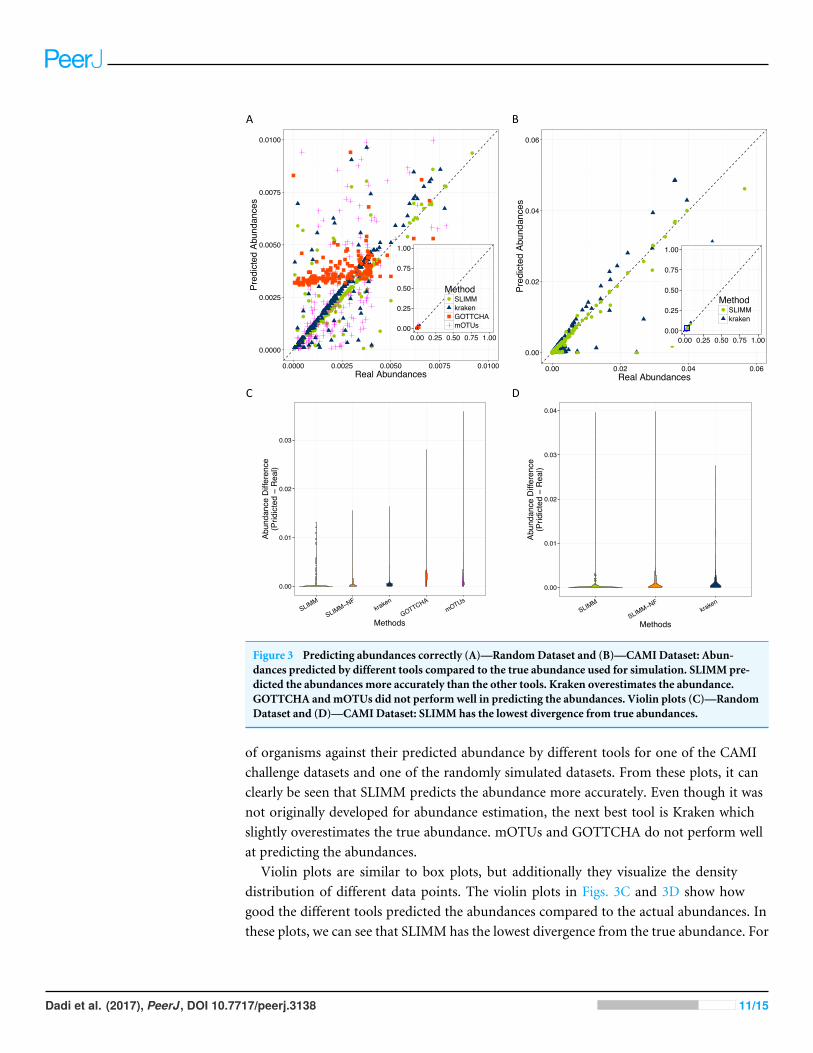
Figure 3 Predicting abundances correctly (A)—RandomDataset and (B)—CAMI Dataset: Abun-dances predicted by different tools compared to the true abundance used for simulation. SLIMM pre-dicted the abundances more accurately than the other tools. Kraken overestimates the abundance.GOTTCHA andmOTUs did not perform well in predicting the abundances. Violin plots (C)—RandomDataset and (D)—CAMI Dataset: SLIMM has the lowest divergence from true abundances.

of organisms against their predicted abundance by different tools for one of the CAMIchallenge datasets and one of the randomly simulated datasets. From these plots, it canclearly be seen that SLIMM predicts the abundance more accurately. Even though it wasnot originally developed for abundance estimation, the next best tool is Kraken whichslightly overestimates the true abundance. mOTUs and GOTTCHA do not perform wellat predicting the abundances.

Violin plots are similar to box plots, but additionally they visualize the densitydistribution of different data points. The violin plots in Figs. 3C and 3D show howgood the different tools predicted the abundances compared to the actual abundances. Inthese plots, we can see that SLIMM has the lowest divergence from the true abundance. For

Dadi et al. (2017), PeerJ, DOI 10.7717/peerj.3138 11/15

the randomly simulated dataset, SLIMM has an average absolute difference of 0.00073 andKraken has an average absolute difference of 0.00116 which is 159% higher compared toSLIMM. For the same dataset, GOTTCHA andmOTUs have an average absolute differenceof 0.00206 and 0.00273 respectively. SLIMM also received the most correct (closer)abundances with absolute differences of first quartile (Q1)= 0.00002 and third quartile(Q3)= 0.00016. Kraken is the second-best tool in this regard with values Q1= 0.00018,Q3= 0.00065.

We have also investigated the positive effects of the filtering step in SLIMM. We ranSLIMM with the filter turned off and compared the results with a standard run of SLIMM.Figures 2C and 2D show that the filtration step overall leads to better results. It is alsointeresting to note that SLIMM’s filtration step effectively reduces the divergence fromthe true abundance. Figures 3C and 3D show that SLIMM’s filtration step producedabundances closer to the real one. The quartiles of absolute differences between real andpredicted abundances are (Q1= 0.00002, Q2= 0.00004, Q3= 0.00016) with filtrationcompared to (Q1= 0.00002, Q2= 0.00006, Q3= 0.00082) without filtration. See thesupplement for more plots on the other datasets.

In conclusion, we described a method that results in a simple, fast and scalable toolfor taxonomic profiling and abundance estimation which utilizes coverage information ofindividual genomes to filter out those that are unlikely to be in the sample. This is doneby discarding genomes with relatively low coverage percentage by uniquely mapped readsand mapping reads in general. These simple yet important filtration steps allow SLIMMto be capable of identifying organisms with high recall rate while remaining precise. Weshowed that SLIMMmethodology resulted in more accurate taxonomic profiling as well aspredicting the individual abundance of member organisms more accurately than the othertools. We evaluated the accuracy of SLIMM against Kraken, GOTTCHA andmOTUs using18 different datasets from multiple sources. The results show that SLIMM is superior indetecting the correct member organisms of a microbial community. SLIMM exhibited thehighest F1-Score in 17 out of the 18 cases. The average F1-score across the datasets is 0.93 forSLIMM, 0.77 for Kraken, 0.54 for GOTTCHA and 0.49 for mOTUs.We have also evaluatedthe correctness of individual abundances using average absolute difference of predictedabundance from the true abundance. SLIMM has the lowest average absolute difference(0.00073) of all the othermethods and the next best tool in this regard is Krakenwith averageabsolute difference of 0.00116. Regarding runtime and memory consumption, SLIMM isthe fastest tool, without the preprocessing step, while using significantly less memory. Theseadvances on taxonomic profiling of microbial communities will help determine the alpha(community level) diversity and beta diversity acrossmultiplemicrobial communitiesmorereliably. This in-turn better facilitate follow-up studies such as the impacts of antibioticusage on microbial communities and consequently on the host’s health.

ACKNOWLEDGEMENTSWe would like to thank Martin Lindner for his helpful discussions and ideas on the subjectmatter. We also thank the reviewers for their constructive comments.

Dadi et al. (2017), PeerJ, DOI 10.7717/peerj.3138 12/15

ADDITIONAL INFORMATION AND DECLARATIONS

FundingThis work is supported by the InternationalMax PlanckResearch School for ComputationalBiology and Scientific Computing and by the InfectControl 2020 Project (TFP-TV4). Thefunders had no role in study design, data collection and analysis, decision to publish, orpreparation of the manuscript.

Grant DisclosuresThe following grant information was disclosed by the authors:International Max Planck Research School for Computational Biology and ScientificComputing and by the InfectControl 2020 Project: TFP-TV4.

Competing InterestsThe authors declare there are no competing interests.

Author Contributions• Temesgen Hailemariam Dadi conceived and designed the experiments, performed theexperiments, analyzed the data, wrote the paper, prepared figures and/or tables, revieweddrafts of the paper.• Bernhard Y. Renard, Lothar H. Wieler and Torsten Semmler wrote the paper, revieweddrafts of the paper.• Knut Reinert wrote the paper, prepared figures and/or tables, reviewed drafts of thepaper.

Data AvailabilityThe following information was supplied regarding data availability:

SLIMM was developed in C++ with SeqAn Library (Döring et al., 2008). The program isavailable for free at https://github.com/seqan/slimm.

Supplemental InformationSupplemental information for this article can be found online at http://dx.doi.org/10.7717/peerj.3138#supplemental-information.

REFERENCESBrady A, Salzberg SL. 2009. Phymm and PhymmBL: metagenomic phylogenetic

classification with interpolated Markov models. Nature Methods 6(9):673–676DOI 10.1038/nmeth.1358.

Brown CT, Howe A, Zhang Q, Pyrkosz AB, Brom TH. 2012. A reference-free algorithmfor computational normalization of shotgun sequencing data. ArXiv preprint.arXiv:1203.4802.

Döring A,Weese D, Rausch T, Reinert K. 2008. SeqAn an efficient, generic C++ libraryfor sequence analysis. BMC Bioinformatics 9:11 DOI 10.1186/1471-2105-9-11.

Dadi et al. (2017), PeerJ, DOI 10.7717/peerj.3138 13/15

Francis OE, Bendall M, Manimaran S, Hong C, Clement NL, Castro-Nallar E, Snell Q,Schaalje GB, Clement MJ, Crandall KA, JohnsonWE. 2013. Pathoscope: speciesidentification and strain attribution with unassembled sequencing data. GenomeResearch 23(10):1721–1729 DOI 10.1101/gr.150151.112.

Freitas TA, Li PE, Scholz MB, Chain PS. 2015. Accurate read-based metagenomecharacterization using a hierarchical suite of unique signatures. Nucleic AcidsResearch 43(10):e69 DOI 10.1093/nar/gkv180.

HMPC. 2012. A framework for human microbiome research. Nature 486(7402):215–221DOI 10.1038/nature11209.

Jia B, Xuan L, Cai K, Hu Z, Ma L,Wei C. 2013. NeSSM: a next-generation sequencingsimulator for metagenomics. PLOS ONE 8(10):e75448DOI 10.1371/journal.pone.0075448.

Langmead B, Salzberg SL. 2012. Fast gapped-read alignment with Bowtie 2. NatureMethods 9(4):357–359 DOI 10.1038/nmeth.1923.

Lindgreen S, Adair KL, Gardner PP. 2016. An evaluation of the accuracy and speed ofmetagenome analysis tools. Scientific Reports 6:19233 DOI 10.1038/srep19233.

Lindner MS, KollockM, Zickmann F, Renard BY. 2013. Analyzing genome coverageprofiles with applications to quality control in metagenomics. Bioinformatics29(10):1260–1267 DOI 10.1093/bioinformatics/btt147.

Lindner MS, Renard BY. 2015.Metagenomic profiling of known unknown microbeswith MicrobeGPS. PLOS ONE 10(2): e0117711.

Oh S, Caro-Quintero A, Tsementzi D, DeLeon-Rodriguez N, Luo C, Poretsky R,Konstantinidis KT. 2011.Metagenomic insights into the evolution, function, andcomplexity of the planktonic microbial community of Lake Lanier, a temperatefreshwater ecosystem. Applied and Environmental Microbiology 77(17):6000–6011DOI 10.1128/AEM.00107-11.

Piro VC, Lindner MS, Renard BY. 2016. DUDes: a top-down taxonomic profiler formetagenomics. Bioinformatics 32(15):2272–2280DOI 10.1093/bioinformatics/btw150.

ShakyaM, Quince C, Campbell JH, Yang ZK, Schadt CW, Podar M. 2013. Comparativemetagenomic and rRNA microbial diversity characterization using archaeal andbacterial synthetic communities. Environmental Microbiology 15(6):1882–1899DOI 10.1111/1462-2920.12086.

Siragusa E. 2013. Approximate string matching for high-throughput sequencing. PhDThesis, Freien Universität Berlin.

Sunagawa S, Mende DR, Zeller G, Izquierdo-Carrasco F, Berger SA, Kultima JR,Coelho LP, ArumugamM, Tap J, Nielsen HB, Rasmussen S, Brunak S, PedersenO, Guarner F, De VosWM,Wang J, Li J, Dore J, Ehrlich SD, Stamatakis A, BorkP. 2013.Metagenomic species profiling using universal phylogenetic marker genes.Nature Methods 10(12):1196–1199 DOI 10.1038/nmeth.2693.

Truong DT, Franzosa EA, Tickle TL, Scholz M,Weingart G, Pasolli E, Tett A, Hut-tenhower C, Segata N. 2015.MetaPhlAn2 for enhanced metagenomic taxonomicprofiling. Nature Methods 12(10):902–903 DOI 10.1038/nmeth.3589.

Dadi et al. (2017), PeerJ, DOI 10.7717/peerj.3138 14/15

Whittaker RH. 1960. Vegetation of the Sisiyou Mountains, Orgeon and California.Ecological Monographs 30:279–338 DOI 10.2307/1943563.

WoodDE, Salzberg SL. 2014. Kraken: ultrafast metagenomic sequence classificationusing exact alignments. Genome Biology 15(3): R46 DOI 10.1186/gb-2014-15-3-r46.

Dadi et al. (2017), PeerJ, DOI 10.7717/peerj.3138 15/15