Sliding mode control of a servo system inLabVIEW: Comparing different control methods

J�anos M�at�e Kiss1, P�eter Tam�as Szemes1p and Petra Aradi2

1 Department of Mechatronics, Faculty of Engineering, University of Debrecen, Debrecen, Hungary2 Department of Mechatronics, Optics, and Mechanical Engineering Informatics, Faculty ofMechanical Engineering, Budapest University of Technology and Economics, Budapest, Hungary

Received: January 24, 2021 • Accepted: March 26, 2021Published online: May 15, 2021

ABSTRACT

The main contribution of this paper is to present the efficiency of LabVIEW in simulating and con-trolling a servo system with conventional methods (PI and PID control), as well as sliding mode control(SMC). The control of an actual system with LabVIEW and NI hardware provides an efficientimplementation platform, using both LabVIEW’s graphical programming and the text-based m-filelanguage MathScript RT. Both programming environments and the connection to NI hardware arerelatively easy to use, therefore, ideal for education. The graphical “coding” can help novice users to seethrough their algorithms. However, the mathematical background of sliding mode control is difficultcompared to conventional PID control; the SMC implementation for practical uses can be quite simple,as the presented example demonstrates. The first didactic step is a simulation with the Control Designand Simulation, as well as MathScript RT Modules. Then a myRIO Student Embedded Device is used tocontrol a real servo system. LabVIEW code can be compiled to run on computers, (soft) real-timetargets, and FPGAs (hard real-time targets), so students can easily and quickly step up to real industrialmeasurement and control problems without the need to learn new programming environments.

KEYWORDS

DC servo motor, PI and PID control, sliding mode control, simulation, real-world system, measurement, LabVIEW,education

1. INTRODUCTION

Simulating control systems helps students understand control methods better than writtentextbook examples. The ability to experiment with the effects of different control strategies onreal-world processes is even more helpful. Conventional PID control is part of the controlengineering curriculum for bachelor-level courses. However, the more robust but mathe-matically far more challenging sliding mode control is usually introduced later in graduatestudies.

Permanent-magnet brushed DC motors, and servo drives are widespread in industry andDIY home projects, ranging from low-power versions to vehicle drive systems. Both speedand position control are possible with a wide range of controllers, with the most commoncontrol method being PI or PID [1, 2]. PI and PID control usually satisfies the most commonrequirements. However, when the system has a variable load, rather than nominal ones, usinga PI or PID controller does not result in a fast and stable output voltage response.

Another possible method is sliding mode control (SMC). Because of the switchingbehaviour of sliding mode control, it is commonly used in power electronics [3–5].

SMC is usually referred to as an interesting theory, as the mathematical model itself worksvery well on a theoretical level, but implementation can be a significant challenge. In theliterature, some hybrid solutions are reported to overcome this problem [3, 6].

The project aims to implement PI, PID, and SMC control of a DC servo system, both as asimulation and real-world measurement. This simple system can be used as a teaching tool.

International Review ofApplied Sciences andEngineering

12 (2021) 2, 201–210

DOI:10.1556/1848.2021.00250© 2021 The Author(s)

ORIGINAL RESEARCHPAPER

pCorresponding author.E-mail: szemespeter@eng.unideb.hu

Unauthenticated | Downloaded 01/16/22 08:31 PM UTC

The chosen programming environment is National In-struments (NI) LabVIEW, a graphical programming envi-ronment with excellent hardware connections to real-worldprocesses. LabVIEW programming is similar to drawing thealgorithm’s block diagram with user interface elementsrepresented as nodes, programming structures such as loops,and built-in functions and procedures. The Control Designand Simulation Module consists of many VIs (Virtual In-struments, the name of LabVIEW subroutines) for controltheory applications, both in time- and frequency domain.Simulation loops provide a graphical model definition,similar to the one in Simulink, and are used to the timestepby timestep simulation of various dynamical systems. TheMathScript RT Module is a text-based m-file programmingenvironment incorporated into LabVIEW. MathScript canbe used as an individual application that functions similarlyto MATLAB. MathScript text-based codes can also be usedwithin a graphical LabVIEW program when inserted into aso-called MathScript Node that acts as a VI.

LabVIEW can interface with measurement and auto-mation products from various manufacturers, besides de-vices from LabVIEW’s developer National Instruments. NIhas specific hardware products for students, such as themyRIO Student Embedded Device that was chosen for themeasurement and control of the real-world DC servo sys-tem. The servo system was first simulated in LabVIEW. PI,PID, and SMC control methods were programmed in Lab-VIEW/MathScript, and various experiments were performedto evaluate the control strategies. Implementing the simu-lation and measurement setup is relatively simple; the pro-gramming environment is clear-cut and self-explaining.LabVIEW does not require long to learn; therefore, it isexcellent for demonstrational purposes in higher-level edu-cation. There are even versions of LEGO robots, e.g. Ro-botics Invention System that shipped with a specialLabVIEW version. Further gain by using LabVIEW is thatthe developed controller code can be compiled to run notjust on computers but (soft) real-time targets and FPGAs(hard real-time targets). That way, students can easily andquickly step up from computer simulation to real industrialmeasurement and control problems without the need tolearn new programming environments.

The presented example of the sliding mode control is farfrom the complex industrial applications; however, themeasurement setup provides an excellent possibility tointroduce the basics of this control method with an existingphysical system even for bachelor-level students. The DC-motor system can further be used to test other controlstrategies both with the simulated and the actual process.

2. PI AND PID CONTROLLERS

The PI or PID controller is the most used solution for con-trolling the speed of motors. Their operation is based on errorsignal compensation. They consist of a total of two or threeparallelly connected terms whose initials give their name. Pstands for proportional, I for integrating, and D for derivative.

The output of the proportional term is proportional to theerror signal, the integrating term is proportional to the integralof the error signal, and the derivative term is proportional tothe derivative of the error signal. As the gain of the propor-tional member increases, the value of the control signal andwith it the error increase proportionally. The controller will tryto respond faster to the error signal, but at the same time, theovershoot will also increase. With the help of the integratingmember, not only the rise time but also the steady-state errorcan be reduced. The disadvantage is that it can slow down thesystem and cause oscillations when the sign of the error signalchanges because it may take some time to follow it. The outputof the PI controller is described by Eq. (1).

uðtÞ ¼ Kp$eðtÞ þ Ki$

Z t

0eðτÞdτ (1)

Kp is the gain of the proportional term, e is the error signalgiven by the difference between the setpoint (referencesignal) and the process variable, Ki is the gain of the inte-grating term, and τ is the integration time.

By adding a derivative term, the controller can predict theerror in advance. It can be used to amplify the control signalwhile keeping the amplitude of the error relatively small. Thiswill dampen the system and reduce overshoot while notaffecting the steady-state error. The output of a complete PIDcontroller supplemented with a derivative term is describedby Eq. (2), where Kd is the gain of the derivative term.

uðtÞ ¼ Kp$eðtÞ þ Ki$

Z t

0eðτÞdτ þ Kd$

deðtÞdt

(2)

There are other mathematical representations of the PID-controller’s transfer function; in LabVIEW the transferfunction version of Eq. (2) is called Parallel, with thefollowing parameters:

Kc þ 1Tis

þ Tds (3)

The other two formats are Academic:

Kc

�1þ 1

Tisþ Tds

�(4)

and Series:

Kc

�1þ 1

Tis

�ð1þ TdsÞ (5)

The low-pass filter of the derivative term can be specifiedwith the a parameter, in each representation, when appro-priate:

1aTdsþ 1

(6)

3. SLIDING MODE CONTROL

Sliding mode control was developed in the Soviet Union pri-marily for aerospace and missile applications in the 1970s [7,8]. The mathematical basis of SMC design can be found in [9].

202 International Review of Applied Sciences and Engineering 12 (2021) 2, 201–210

Unauthenticated | Downloaded 01/16/22 08:31 PM UTC

Although understanding the exact mathematicaldescription behind the method can be challenging, in manycases, it is relatively easy to apply SMC without a deeperknowledge of its complex mathematical background.Because of this and its robustness, it is widespread, forexample, in robotics, power electronics, and servo drivecontrol, where variable system structures are common [3–5,10].

SMC’s aim is to bring the system into a state in whichits dynamics can be described by a differential equationwith a lower degree of freedom, in which case, in theory,the system is completely independent of changes in certaintypes of parameters and certain types of external distur-bances. This condition is called sliding mode. Although,according to the theory, sliding mode control appears to bea well-functioning and robust control method, unfortu-nately, there are severe limitations to its practical imple-mentation. The main problem is the so-called chattering[11], which means a high-frequency oscillation around thesliding surface that significantly reduces the efficiency androbustness of the controller. While, in theory, SMC pro-vides superior performance of the closed-loop system insliding mode, the practical limitations discourage someresearchers. The need for higher sampling frequency thanother control strategies to reduce the high-frequencyoscillation phenomenon (chattering) is the limiting factor.There are approaches to overcome this problem, such asan observer-based, discrete-time, sliding mode controldesign that prevents the system from entering the criticaldomain [12, 13].

The first step in designing a sliding mode controller is todefine the sliding surface. The sliding surface is as follows:

s ¼�deðtÞdt

þ C$eðtÞ�n−1

(7)

s is the sliding surface, C is a strictly positive constant thatdetermines the bandwidth of the system (also mentioned asλ in some literature), n is the degree of the system, and e isthe error signal. The transfer function of the brushed DCmotor is second degree, so by substituting the speed, thesliding surface is obtained as follows:

s ¼ dueðtÞdt

þ C$ue (8)

Rotational speed ue is the error signal defined as thedifference between the reference signal and the processvariable. Once the sliding surface has been determined, thenext step is to create a control signal with which the slidingsurface can be reached and maintained. This is subject to:

s$ _s>0 (9)

In order to satisfy this condition, the principle of thediscontinuous controller output signal is obtained with thesign function, where the variable is the instantaneous valueof the sliding surface and K is a positive constant:

u ¼ K$sgnðsÞ (10)

The sign (sgn) function in (6) is defined as

s ¼�

−1; s<0þ1; s≥ 0

(11)

The use of the sign function may lead to chattering, whichcan have a harmful effect on the motor, so avoiding thisphenomenon is very important for SMC. One method toprevent chattering is to replace the sign function with thepseudo function:

u ¼ K$s

jsj þ d(12)

where d is a small positive constant called a tuning param-eter to reduce the chattering [14]. The choice of d is a crucialconsideration because if it is too small, the chattering maystill be present, but if it is too large, reaching the referencevalue may cause a problem to the controller [15].

Figure 1 shows the MathScript implementation of thesliding mode controller as a LabVIEW MathScript Nodewith inputs on the left side and the controller output on theright side of the frame.

4. LABVIEW MOTOR MODEL

The transfer functions of the DC motor’s electrical andmechanical characteristics can be created using the built-infunction block of the Construct Transfer Function ModelVI. The numerator of the transfer function is given by theconstant value of 1, and the denominator consists of anindexed array, the elements of which are read from thecluster containing the motor parameters in SI units(Table 1). The symbols are as follows: armature resistanceand inductance are denoted by Ra and La, respectively. J isthe moment of inertia, and B represents the friction coeffi-cient. Kv is the back-EMF constant, and Kt is the torqueconstant. The transfer function elements are listed indescending order of degree. In the next step, the generatedtransfer function is converted by the Convert ControlDesign to Simulation VI function block to a form that can beused in the simulation loop (Fig. 2).

The block diagram of Fig. 2 represents the transferfunction between the motor’s voltage input and rotationalspeed output (the integrator labelled Position calculates the

Fig. 1. Calculation of the control signal of the sliding modecontroller

International Review of Applied Sciences and Engineering 12 (2021) 2, 201–210 203

Unauthenticated | Downloaded 01/16/22 08:31 PM UTC

integral of rotational speed and is not included in thefollowing transfer function):

GðsÞ ¼ Kt

ðLsþ RÞðJsþ BÞ þ KtKv(13)

Each parameter can be saved or loaded in XML format forthe repeatability of the simulations. The XML file’s path canbe input via the program’s user interface or hard-coded intothe program. The parameters can be validated by pressingthe apply button.

The model’s correct behaviour can be tested with severaltest functions available in LabVIEW, or the user can create anown test VI. A function generator has been placed in theprogram, which can be freely configured in the user interfaceto create several general test signals. Configurable parametersare duty cycle, period, amplitude, and offset. An Express VI isalso included in the program to save the simulation data to anxlsx spreadsheet file. The current time of the simulation, the

current value of the test signal, the motor speed, the current,and the position is stored in the file after each iteration.

The simulation results obtained with each parameter areshown in Fig. 3.

5. SIMULATION RESULTS

The controller parameters were determined with LabVIEW’sControl Design and Simulation Module’s built-in tuningblocks for the PI and PID controllers with the use of variousavailable tuning methods (ZN: Ziegler-Nichols, CC: Cohen-Coon, CHR: Chien-Hrones-Reswick, IMC: Internal ModelControl). The details of these tuning methods are availablein the official user manual and help.

The controller parameters determined by Internal ModelControl are used, as this method gave the fastest operation,according to the simulation results. The parameters of the PIand PID controllers are shown in Table 2.

The parameter values of the sliding mode controller areC 5 10, K 5 40 and d 5 0.05.

5.1. Step function

The first test for each controller was a step function test inwhich the speed setpoint jumped from 0 to 10 rad/s in thefirst second of the simulation. The speed responses obtainedfor this are summarized in Fig. 4.

Table 1. Parameters of motors for the transfer function

Parameter Test1 Test2 Test3

Ra 2 0.6 1La 0.5 0.8 0.2Kt 0.1 0.2 0.2Kv 0.1 0.2 0.8J 0.2 0.9 0.4B 0.02 0.7 0.5

Fig. 2. Block diagram of the model

204 International Review of Applied Sciences and Engineering 12 (2021) 2, 201–210

Unauthenticated | Downloaded 01/16/22 08:31 PM UTC

The simulation results in Table 3 show that the theoreticaldifferences between controllers are significant. As expected,the PI controller is the slowest and has the most extensiveovershoot. The PID, which has an additional derivativemember, produced a slightly smaller overshoot, and both therise and settling times are shorter. Of the three controllers, thesliding mode controller performed outstandingly well. Boththe rise and settling times are quicker than the PI and PIDcontrollers, and there is no overshoot.

The phase margin value was nearly identical for the PIand PID controller: 53.368 for PI and 53.738 for PID.

Figure 5 shows the control signal for different controllerswith the characteristic alternating in the sliding mode con-troller’s control signal and the PID controller’s relativelylarge initial value.

Figure 6 shows the error and error derivative plots of thedifferent controllers with the two distinctive parts for thesliding mode controller.

5.2. Tracking

In this case, the initial value of the speed reference signal is10 rad/s, and after the steady-state is reached, it is changedabruptly to 5 rad/s in the fifth second. The comparison isshown in Fig. 7. The results again reflect the differencedescribed in theory as in the previous case of the stepfunction. The sliding mode control was spectacularly betterin this study as well, as it was able to follow the change of thereference signal the fastest and to reach the new steady-stateasymptotically. The tracking results show similar perfor-mance to step response results. Sliding mode control per-formed best; the undershoot and settling time of the loopwith the PID controller were smaller than those of the onewith the PI controller.

5.3. Speed function

In the case of the speed function, the result is similar to theprevious ones; the sliding mode controller performed best,as it was able to follow the signal almost perfectly in the caseof the ideal motor model. The difference between PI andPID controllers is as expected from the theory. The response

Fig. 3. Results of motor model testing with different parameters

Table 2. Parameters of controllers

Parameter Controller ZN CC CHR IMC

Kc PI 2.120 2.228 1.413 2.356PID 2.635 3.466 2.238 6.011

Ti (min) PI 0.012 0.006 0.014 0.006PID 0.007 0.007 0.008 0.008

Td (min) PI – – – –PID 0.002 0.001 0.001 0.001

Fig. 4. Comparison of controllers with step function

Table 3. Simulation results

ControllerRise time

(s)Settlingtime (s)

Overshoot(%)

Undershoot(%)

PI 0.395 1.977 13.56 4.97PID 0.326 1.687 11.61 5.17SMC 0.281 0.591 – –

Fig. 5. The control signal of different controllers

International Review of Applied Sciences and Engineering 12 (2021) 2, 201–210 205

Unauthenticated | Downloaded 01/16/22 08:31 PM UTC

of the controllers is shown in Fig. 8. For the comparison, theresults of the best performers were used, so in the case of thePI controller, the curves obtained with the smallest averageerror are Cohen-Coon, while in the case of the PIDcontroller, the curves were obtained with the parameters ofthe Internal Model Control method.

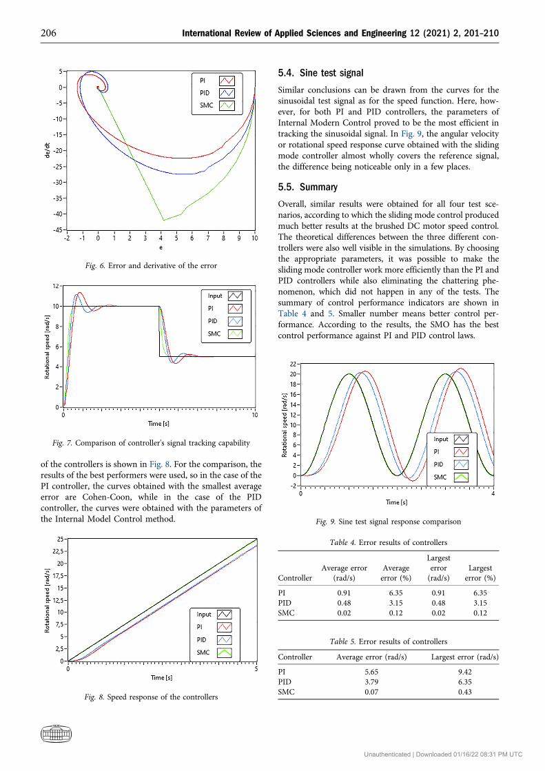
5.4. Sine test signal

Similar conclusions can be drawn from the curves for thesinusoidal test signal as for the speed function. Here, how-ever, for both PI and PID controllers, the parameters ofInternal Modern Control proved to be the most efficient intracking the sinusoidal signal. In Fig. 9, the angular velocityor rotational speed response curve obtained with the slidingmode controller almost wholly covers the reference signal,the difference being noticeable only in a few places.

5.5. Summary

Overall, similar results were obtained for all four test sce-narios, according to which the sliding mode control producedmuch better results at the brushed DC motor speed control.The theoretical differences between the three different con-trollers were also well visible in the simulations. By choosingthe appropriate parameters, it was possible to make thesliding mode controller work more efficiently than the PI andPID controllers while also eliminating the chattering phe-nomenon, which did not happen in any of the tests. Thesummary of control performance indicators are shown inTable 4 and 5. Smaller number means better control per-formance. According to the results, the SMO has the bestcontrol performance against PI and PID control laws.

Fig. 6. Error and derivative of the error

Fig. 7. Comparison of controller's signal tracking capability

Fig. 8. Speed response of the controllers

Table 5. Error results of controllers

Controller Average error (rad/s) Largest error (rad/s)

PI 5.65 9.42PID 3.79 6.35SMC 0.07 0.43

Fig. 9. Sine test signal response comparison

Table 4. Error results of controllers

ControllerAverage error

(rad/s)Averageerror (%)

Largesterror(rad/s)

Largesterror (%)

PI 0.91 6.35 0.91 6.35PID 0.48 3.15 0.48 3.15SMC 0.02 0.12 0.02 0.12

206 International Review of Applied Sciences and Engineering 12 (2021) 2, 201–210

Unauthenticated | Downloaded 01/16/22 08:31 PM UTC

6. MEASUREMENT AND CONTROL SYSTEMWITH A REAL MOTOR

The main components of the physical system are the powersupply, the NI myRIO Student Embedded Device, thatserves as the interface between the real-world system and thecomputer running the LabVIEW code, the motor drivecircuit, the permanent magnetic brush DC electric motor,and the speed feedback encoder. The assembly is illustratedin Fig. 10. The myRIO has dedicated inputs correspondingto terminals A and B of the quadratic encoder, which aredigital inputs DIO18 and DIO22. It also contains dedicatedoutputs for the PWM signal, for which the digital outputDIO27/PWM0 has been used. A 5V high signal is requiredon the motor drive circuit to turn on the motor, which isspecified at output DIO13.

The main parameters of the motor are summarized inTable 6.

Figure 11 shows part of the LabVIEW program used inthe experimental setup. The encoder’s signal represents theprocess value. The reference signal and process value are theinputs of the PID controller block, together with the PIDparameters, that come from the tuning process. The PIDblock’s output is the control signal connected to the DC-motor’s input via the PWM block. This typical LabVIEW“program code” illustrates the ease of use and transparencyof LabVIEW applications with connected hardware com-ponents via a connecting device, in this example, a myRIOStudent Embedded Device.

7. RESULTS WITH THE REAL MOTOR

Real-world measurements differ from the simulation inmotor parameters that result in different timescales, test

signals, and instead of rotational speed in rad/s, RPM in1/min is used. It is somewhat intentional because studentsare required to analyse results and implement the simula-tion with the experiments’ parameters, not just checkwhether the simulated results look like the real-worldmeasurements.

In the real DC-motor system PI and PID controllers areimplemented with the built-in VIs, like in the case of theideal motor model. It is important to note that the step sizeof the simulation and the step size of the PID VI must beconsistent so that the instantaneous speed is calculatedcorrectly from the encoder signal. The definition of theparameters and the operation of the program are the same asthose used for the ideal model. The parameters determinedfor each controller with the use of various tuning methodsare summarized in Table 7.

The sliding mode control parameters this time are C5 2,K 5 1 and d 5 0.9. The value of K determines the range ofthe output and since the duty cycle can take a value between0 and 1 according to the Express VI used, it also determinesthe value of the parameter. The value of C was determinedempirically, in the case of further increase, the control wasnot functional, and the value of d still had to be chosen to be0.9.

Responses to various test scenarios are shown inFigs 12–15. It is important to note that the results seem toshow the effect of saturation that was not present in thesimulation.

Fig. 10. The measuring system

Table 6. Parameters of the real motor

Resistance [Ω] 2.32Inductance [mH] 0.238Speed constant [(1/min)/V] 408Torque constant [m Nm/A] 23.4Rotor inertia [g cm2] 10.8

International Review of Applied Sciences and Engineering 12 (2021) 2, 201–210 207

Unauthenticated | Downloaded 01/16/22 08:31 PM UTC

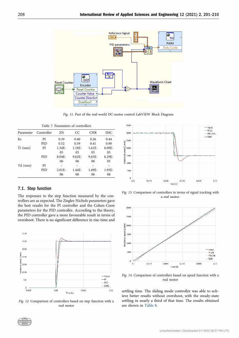
7.1. Step function

The responses to the step function measured by the con-trollers are as expected. The Ziegler-Nichols parameters gavethe best results for the PI controller and the Cohen-Coonparameters for the PID controller. According to the theory,the PID controller gave a more favourable result in terms ofovershoot. There is no significant difference in rise-time and

settling time. The sliding mode controller was able to ach-ieve better results without overshoot, with the steady-statesettling in nearly a third of that time. The results obtainedare shown in Table 8.

Table 7. Parameters of controllers

Parameter Controller ZN CC CHR IMC

Kc PI 0.39 0.40 0.26 0.44PID 0.52 0.59 0.41 0.90

Ti (min) PI 1.34E-05

1.18E-05

1.61E-05

6.09E-05

PID 8.04E-06

9.62E-06

9.65E-06

6.29E-05

Td (min) PI – – – –PID 2.01E-

061.44E-06

1.69E-06

1.95E-06

Fig. 11. Part of the real-world DC-motor control LabVIEW Block Diagram

Fig. 12. Comparison of controllers based on step function with areal motor

Fig. 13. Comparison of controllers in terms of signal tracking witha real motor.

Fig. 14. Comparison of controllers based on speed function with areal motor

208 International Review of Applied Sciences and Engineering 12 (2021) 2, 201–210

Unauthenticated | Downloaded 01/16/22 08:31 PM UTC

7.2. Tracking

In tracking the abrupt change of the reference signal. thePID controller performed surprisingly well with the pa-rameters of the Internal Model Control method compared tothe other results.

The sliding mode controller performed best, followed bythe PID and then the PI in the last place. Table 9 shows thecharacteristics of the responses.

7.3. Speed function

For the speed function test signal. the Ziegler-Nichols pa-rameters gave the best results for the PI and PID controllers.

After the start. the error is roughly constant with the PIand PID controllers. while SMC’s error increases more andmore with the increase of the input signal. The properties ofthe response signals are shown in Table 10.

7.4. Sine signal

In the case of the sinusoidal test signal, a better measure-ment result was obtained with the Cohen-Coon parametersat least, however, this difference may also be due to themeasurement error mentioned earlier.

Barely noticeable differences can be seen in Fig. 15; de-tails are presented in Table 11.

8. SUMMARY

When comparing the results of the performed experiments,the sliding mode control worked excellently in the case of theideal theoretical model. For all experiments, SMC was able tofollow the reference signal extremely well for both abruptchanges and continuously changing signals. In the case of PIand PID controllers, there was a significant difference in theparameters determined by different controller tuningmethods, although not all test signals gave the best results.

With the real motor, the sliding mode controller nolonger had a clear advantage. Although in cases where therewas an abrupt change in the reference signal value it hasperformed much better, in the case of continuously changingsignals such as the speed function or the sine signal it hasalready lagged behind the other two controllers.

Simulation is a very useful tool as students can checkvarious controller parameter settings, comparing the results,and, therefore, understand the role of the PID-controller’sparts and their interaction. Experimenting with the tuning ofa simulated control system often provides deeper knowledgethan the use of controller tuning methods from textbookswithout understanding the underlying principles.

The problems of saturation and integral windup usuallyoccur in real-world physical systems. There is an educationalvalue of showing these problems with relatively small-scalereal-world systems without the risk of serious damage, aswell as including the appropriate simulated versions beyondthe idealistic simulated system without considering satura-tion and integral windup. The detailed discussion of satu-ration and integral windup is going to be included in thelaboratory experiments’ handouts soon.

The whole process of modelling the DC servo system,designing controllers and simulating the closed-loop controlsystem, and later performing experiments in a real-worldsystem based on the simulation results has a significanteducational value. Control engineering is considered a rather

Table 8. Results of step input tests

ControllerRise time

(s)Settlingtime(s)

Overshoot(%)

Undershoot(%)

PI 0.0005 0.0017 7.17 –PID 0.0018 4.01 – –SMC 0.0004 0.0006 – –

Table 9. Results of tracking tests

Controller Settling time (s) Undershoot (%) Overshoot (%)

PI 0.0017 24.30 0.78PID 0.0009 4.40 –SMC 0.0001 – –

Table 10. Results of speed function tests

ControllerAverage

error (rad/s)Averageerror (%)

Largesterror (rad/

s)Largesterror (%)

PI 16.50 1.12 71.39 47.56PID 12.37 0.83 63.38 52.72SMC 40.00 2.67 88.80 3.03

Table 11. Results of sine signal tests

Controller Average error (rad/s) Largest error (rad/s)

PI 16.60 26.66PID 11.42 18.47Sliding mode 89.81 149.15

Fig. 15. Comparison of controllers with sinusoidal test signal withreal motor

International Review of Applied Sciences and Engineering 12 (2021) 2, 201–210 209

Unauthenticated | Downloaded 01/16/22 08:31 PM UTC

difficult subject all over the world [16, 17]; therefore, it is wellworth introducing the applications of the theory with exper-iments like the one presented above. As the pandemic situa-tion enforces distant education worldwide, the value andimportance of simulation increases. Students are not allowedto participate in laboratory experiments, so the chance of usingreal-world devices is reduced. Educational devices, such as thepresented NI myRIO, offer the possibility of self-paced ex-periments. especially when students can gain access to them byborrowing or use via the Internet. The expansion of the pre-sented system to Internet access is currently being investigated.

ACKNOWLEDGEMENT

This research was funded by TKS2020-NKA-04. Project no.TKP2020-NKA-04 has been implemented with the supportprovided from the National Research, Development andInnovation Fund of Hungary, financed under the 2020-4.1.1-TKP2020 funding scheme.

REFERENCES

[1] T. Wildi, Electrical Machines. Drives and Power Systems. Upper

Saddle River. NJ. USA: Pearson Prentice Hall, 2006.

[2] G. Sziebig, B. Takarics, and P. Korondi, “Control of an embedded

system via Internet,” IEEE Trans. Ind. Electron., vol. 57, no. 10, pp.

3324–33, Oct. 2010, https://doi.org/10.1109/TIE.2010.2041132.

[3] K. Al-Hosani, A. Malinin, and V. I. Utkin, “Sliding mode PID

control of buck converters,” in 2009 European Control Conference

(ECC), Budapest, 2009, pp. 2740–4, https://doi.org/10.23919/ECC.

2009.7074821.

[4] P. Korondi and H. Hashimoto, “Park vector based sliding mode

control of UPS with unbalanced and nonlinear load,” in Variable

Structure Systems. Sliding Mode and Nonlinear Control, K D. Young

and €U. €Ozg€uner, Eds., London. UK: Springer, 1999, pp. 193–209.

[5] P. Korondi, S. H. Yang, H. Hashimoto, and F. Harashima, “Sliding

mode controller for Parallel resonant dual converters,” J. Circuits.

Syst. Comput., vol. 5, no. 4, pp. 735–46, 1995. https://doi.org/10.

1142/S0218126695000424.

[6] R. E. Precup, S. Preitl, and P. Korondi, “Fuzzy controllers with

maximum sensitivity for servosystems,” IEEE Trans. Ind.

Electron., vol. 54, no. 3, pp. 1298–310, 2007. https://www.doi.org/

10.1109/TIE.2007.893053.

[7] V. I. Utkin and K. D. Yang, “Methods for construction of

discontinuity planes in multidimensional variable structure sys-

tems,” Autom. Remote Control, vol. 39, no. 10, pp. 1466–70, 1979.

[8] K. D. Young, “Controller design for a manipulator using theory of

variable structure systems,” IEEE Trans. Syst. Man. Cybernetics,

vol. 8, no. 2, pp. 101–9, Feb. 1978, https://doi.org/10.1109/TSMC.

1978.4309907.

[9] K. Sz�ell and P. Korondi, “Mathematical basis of sliding mode

control of an uninterruptible power supply,” Acta Polytech.

Hungarica., vol. 11, no. 3. 2014. https://doi.org/10.12700/aph.11.

03.2014.03.6.

[10] P. Korondi and H. Hashimoto, “Sliding mode design for motion

control,” in Applied Electromagnetics and Computational Tech-

nology II : Proceedings of the 5th Japan-Hungary Joint Seminar on

Applied Electromagnetics in Materials and Computational Tech-

nology. IOS Press, 2000, pp. 221–32.

[11] V. Utkin and H. Lee, “Chattering problem in sliding mode control

systems,” IFAC Proc. Volumes, vol. 39, no. 5, p. 1, 2006. https://

doi.org/10.3182/20060607-3-IT-3902.00003.

[12] P. Korondi, H. Hashimoto, and V. Utkin, “Discrete sliding mode

control of two mass system,” in 1995 Proceedings of the IEEE

International Symposium on Industrial Electronics, Athens,

Greece, vol. 1, 1995, pp. 338–43, https://doi.org/10.1109/ISIE.

1995.497019.

[13] P. Korondi, H. Hashimoto, and V. Utkin, “Direct torsion control

of flexible shaft in an observer-based discrete-time sliding mode,”

IEEE Trans. Ind. Electron., vol. 45, no. 2, pp. 291–6, April 1998,

https://doi.org/10.1109/41.681228.

[14] H. Maghfiroh, A. Sujono, M. Ahmad, A. Brillianto, and H.

Chico, “Basic tutorial on sliding mode control in speed control

of DC-motor,” J. Electr. Electron. Inf. Commun. Technol., vol. 2,

no. 1, pp. 1–4, 2020. https://www.doi.org/10.20961/jeeict.2.1.

41354.

[15] E. H. Dursu and A. Durdu, “Speed control of a DC motor with

variable load using sliding mode control,” Int. J. Comput. Electr.

Eng., vol. 8, no. 3, pp. 219–26, 2016. https://www.doi.org/10.

17706/IJCEE.2016.8.3.219-226.

[16] P. Albertos and I. Mareels, Feedback and Control for Everyone.

Berlin, Heidelberg, Germany: Springer, 2010.

[17] K. Zenger, “Control engineering. system theory and mathematics:

the teacher’s challenge,” Eur. J. Eng. Edu., vol. 32, no. 6, pp. 687–94,

2007. https://doi.org/10.1080/03043790701520719.

Open Access. This is an open-access article distributed under the terms of the Creative Commons Attribution 4.0 International License (https://creativecommons.org/licenses/by/4.0/), which permits unrestricted use, distribution, and reproduction in any medium, provided the original author and source are credited, a link to the CCLicense is provided, and changes – if any – are indicated. (SID_1)

210 International Review of Applied Sciences and Engineering 12 (2021) 2, 201–210

Unauthenticated | Downloaded 01/16/22 08:31 PM UTC