slides transmissão de calor

1

Mecanismos FMecanismos Fíísicos esicos eEquaEquaçções de Taxas de ões de Taxas de Transmissão de CalorTransmissão de Calor

• O que éa transferência/transmissão de calor?

A transferência/transmissão de caloré o trânsito de energia térmicadevido a uma diferença de temperaturas num meio ou entre meios.

• O que é aenergia térmica?

A energia térmicaestá associada àtranslação, rotação, vibração e aosestados electrónicosdos átomose moléculasque constituem a matéria.

Transferência de Calor e Energia TTransferência de Calor e Energia Téérmicarmica

A energia térmicarepresenta o efeito cumulativodas actividades microscópicase está relacionada com a temperatura da matéria.

2

UnidadesSímboloSignificado físicoQuantidade

Transporte de energia térmica devido a gradientes de temperatura

Transferência de

Calor

NÃO confundir ou trocar os significados físicos deEnergia Térmica,Temperatura e Transferência de Calor

Energia associada ao comportamento microscópico da matéria

Energia

Térmica+ J/kgJouuU ou

Modo indirecto de determinar a quantidade de energia térmica armazenada na matéria

Temperatura KCº ouT

Quantidade de energia térmica transferida num intervalo de tempo � t > 0

Calor Q J

+ U �� Energia Térmica u �� Energia Térmica específica

Energia térmica transferida por unidade de tempo

Taxa de transferência de calor

q W

Energia térmica transferida por unidade de tempo e por unidade de área

Fluxo de calor 'q' 2/ mW

Condução: Transferência de calor num sólido ou fluido estático (gás ou líquido) devida ao movimento aleatóriodos seus átomos, moléculas e/ou electrões constituintes.

Convecção: Transferência de calor devida ao efeito combinado do movimento aleatório (microscópico)e do movimento macroscópico (advecção)do fluido sobre uma superfície.

Radiação: Energia que éemitida pela matéria devido a mudanças das configurações electrónicas dos seus átomos ou moléculas e que é transportada por ondas electromagnéticas (ou por fotões).

• A condução e a convecção exigem a presença de matéria e de variações de temperatura nesse meio material.

• Embora a radiação tenha origem na matéria, o seu transporte não exige a presença de um meio material. Aliás, o transporte radiativo é mais eficiente no vácuo.

Modos de Transferência de Calor

3

AplicaçõesIdentificaIdentificaçção de mecanismosão de mecanismos

Problema 1.73(a):Identificação de mecanismos de transferência de calor para janelas de vidro simples e duplo

Condução através do vidro que tem superfície interior em contacto com ar exterior na janela de vidro duplo, 2c o n dq

Convecção entre a superfície interior da janela e o ar interior,1co n vqFluxo radiativo útil trocado entre as paredes do quarto e a superfície interior da janela,1ra dq

Condução através do vidro que tem superfície interior em contacto com ar interior,1c o n dq

Radiação solar incidente durante o dia: a fracção transmitida pelo vidro duplo é menor que a transmitida pelo vidro simples. sq

Convecção entre a superfície exterior da janela e o ar exterior,2convq

Fluxo radiativo útil trocado entre a envolvente e a superfície exterior da janela,2radq

Convecção no espaço entre vidros (janela de vidro duplo),conv sq

Fluxo radiativo útil entre as superfícies dos vidros que limitam o espaço entre vidros,rad sq

2 1x

T TdTq k k

dx L

−′′ = − = −

1 2x

T Tq k

L

−′′ =

Taxa de transferência de calor(W): x xq q A′′= ⋅

Aplicação ao caso de condução unidimensional, estacionáriaatravés de umaplaca planacomcondutibilidade térmica constante:

Condução

Forma geral (vectorial) daLei de Fourier:

Taxas de Transferência de Calor

Fluxo de calor(W/m2):

Fluxo de calor2W/m

Condutibilidade térmica

KW/m⋅

Gradiente de temperatura

K/mouC/mº

4

Convecção

Relação entre convecção e o escoamento sobre uma superfície e o desenvolvimentodascamadas limite hidrodinâmica e térmica:

Lei do arrefecimento de Newton:

( )h sq T T∞′′ = −


h [W/m 2.ºC] ou [W/m2.K] : Coeficiente de transferência de calor por convecção


2500 - 100000Ebulição ou condensação

50 - 20000Convecção forçada - líquidos

25 - 250Convecção forçada - gases

50 - 1000Convecção natural - líquidos

2 - 25Convecção natural - gases

Gama de valores típicos do coeficiente de convecção [W m-2 K-1]

• Advecção, difusão, convecção

• Convecção forçada, convecção natural

• Calor sensível e calor latente

• Ebulição e condensação

5

Radiação

Fluxo de energiaque saidevido àemissão:4

b sE E Tε εσ= =

Energiaabsorvidadevida àirradiação: absG Gα=

A transferência de calor por radiaçãonuma interface gás/sólidoenvolve a emissão de radiaçãoa partir da superfície e pode também envolver a absorção da radiação incidenteda envolvente (irradiação, G ), bem como da convecção (se Ts ≠ T∞)


Gabs [W/m2]: Radiação incidente absorvida

αααα (0 ≤≤≤≤ αααα ≤≤≤≤ 1): Absorsividade da superfície

G [W/m 2]: Irradiação

E [W/m2]: Poder emissivo da superfícieεεεε (0 ≤≤≤≤ εεεε ≤≤≤≤1): Emissividade da superfícieEb [W/m2]: Poder emissivo de um corpo negro (emissor perfeito)σσσσ = 5,67××××10-8 [W m -2 K -4] (constante de Stefan-Boltzmann)

Irradiação : Caso especialde uma superfície exposta a uma envolvente de grandes dimensões com temperatura uniforme,surT

4sur surG G Tσ= =


Se αααα = εεεε, o fluxo radiativo útil a partir da superfície

devido às trocas de calor por radiação com a envolvente é:

( ) ( )4sur

4sSb

''rad TTσεGαTEεq −=−=

6

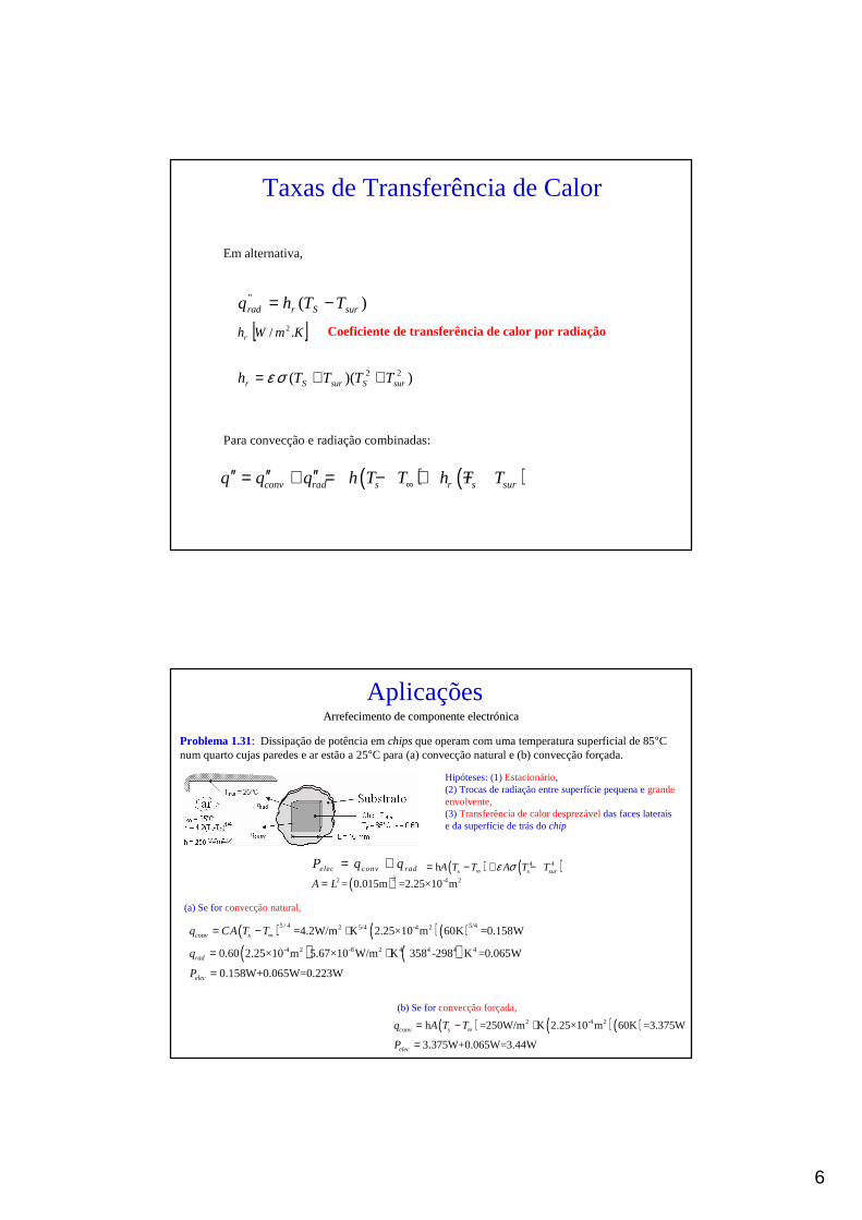
Em alternativa,

Para convecção e radiação combinadas:

( ) ( )conv rad s r s surq q q h T T h T T∞′′ ′′ ′′= + = − + − (1.10)


))(( 22surSsurSr TTTTh ++= σε

)(''surSrrad TThq −=

[ ]KmWhr ./ 2 Coeficiente de transferência de calor por radiação

AplicaçõesArrefecimento de componente electrArrefecimento de componente electróónicanica

Problema 1.31: Dissipação de potência em chipsque operam com uma temperatura superficial de 85°C num quarto cujas paredes e ar estão a 25°C para (a) convecção natural e (b) convecção forçada.

Hipóteses: (1)Estacionário, (2) Trocas de radiação entre superfície pequena e grande envolvente, (3) Transferência de calor desprezável das faces laterais e da superfície de trás do chip

( ) ( )4 4h s s surA T T A T Tε σ∞= − + −elec conv radP q q= +( )22 -4 2= 0.015m =2.25×10 mA L=

(a) Se forconvecção natural,

( ) ( )( )( ) ( )

5 / 4 5/42 5/4 -4 2

-4 2 -8 2 4 4 4 4

=4.2W/m K 2.25×10 m 60K =0.158W

0.60 2.25×10 m 5.67×10 W/m K 358 -298 K =0.065W

0.158W+0.065W=0.223W

conv s

rad

elec

q CA T T

q

P

∞= − ⋅

= ⋅

=

(b) Se forconvecção forçada,

( ) ( )( )2 -4 2h =250W/m K 2.25×10 m 60K =3.375W

3.375W+0.065W=3.44W

conv s

elec

q A T T

P

∞= − ⋅

=

7

ConservaConservaçção de Energiaão de Energia

•Formulações Alternativas

Base temporal:

Num instanteouNum intervalo de tempo

Tipo de Sistema:

Volume de controloSuperfície de controlo

• Uma ferramenta importante na análise do fenómeno de transferência de calor, constituindo geralmente a base para determinar a temperaturado sistema em estudo.

CONSERVAÇÃO DE ENERGIA(Primeira Lei da Termodinâmica)

8

•• Num instante de tempo:Num instante de tempo:

Notar a representação do sistema através de umasuperfície de controlo (linha a tracejado)nas fronteiras.

Fenómenos superficiais

Fenómenos volumétricos

APLICAÇÃO A UM VOLUME DE CONTROLO

Taxa de transferência de energia térmica e/ou mecânica através da superfície de controlo, devido à transferência de calor, escoamento de um fluido ou transferência de trabalho

Taxa de geração de energia térmicadevido à conversão de outra forma de energia (e.g. eléctrica, nuclear, química); conversão essa de energia que ocorre no interior do sistema

Taxa de variação de energia armazenada no sistema

•• Num instante de tempo:Num instante de tempo:

Notar a representação do sistema através de umasuperfície de controlo (linha a tracejado line)nas fronteiras.

Conservação de energia

APLICAÇÃO A UM VOLUME DE CONTROLO

• Num intervalo de tempo:

( )bEEEE stoutgin 11.1∆=−+ Cada termo tem unidades [J].

Cada termo tem unidades [J/s] ou [W].

9

Há um caso especial para o qual não existe massa ou volume contidos na superfície de controlo

Conservação de Energia (num instante):

• Aplica-se em condições estacionárias e transientes

Considere a superfície de uma parede com transferência de calor (condução, convecção e radiação).

0cond conv radq q q′′ ′′ ′′− − =

( ) ( )4 41 22 2 2 0sur

T Tk T T T T

Lε σ∞

− − − − − =h

• Sem massa nem volume, não faz sentido falar em energia armazenada ou em geração no balanço de energia, mesmo que estes fenómenos ocorram no meio de que a superfície faz parte.

O BALANÇO DE ENERGIA SUPERFICIAL

0=− outin EE &&

EXEMPLOS DE APLICAÇÃO

Exemplo 1.3: Aplicação à resposta térmica de um fio condutor com aquecimento por efeitode Joule (geração de calor à passagem da corrente eléctrica).

0=inE& ( ) ( ) ( )[ ]44surout TTTThLDE −+−= ∞ σεπ&

2IRE electg =& ( )TVctd

dEst ρ=&

stgoutin EEEE &&&& =+−

10


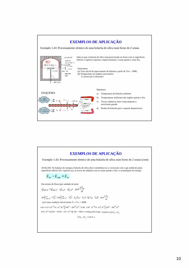
Exemplo 1.43: Processamento térmico de uma bolacha de sílica num forno de 2 zonas.

Sabe-se que a bolacha de sílica está posicionada no forno com as superfícies inferior e superior expostas, respectivamente, à zona quente e zona fria.

Determinar (a) Taxa inicial de aquecimento da bolacha a partir de Twi = 300K, (b) Temperatura em regime estacionário.

A convecção é relevante?

ESQUEMAHipóteses:

a) Temperatura da bolacha uniforme

b) Temperaturas uniformes das regiões quente e fria

c) Trocas radiativas entre corpo pequeno e envolvente grande

d) Perdas da bolacha para o suporte desprezáveis


Exemplo 1.43: Processamento térmico de uma bolacha de sílica num forno de 2 zonas (cont)

ANÁLISE: No balanço de energia à bolacha de sílica deve contabilizar-se a convecção com o gás ambiente pelas superfícies inferior (l) e superior (u), as trocas de radiação com as zonas quente e fria e a acumulação de energia.

, , , ,w

rad h rad c cv u cv ld T

q q q q cddt

ρ′′ ′′ ′′ ′′+ − − =

Em termos de fluxo (por unidade de área)

( ) ( ) ( ) ( )4 4 4 4,,

ww sur c w u w l wsur h

d TT T T T h T T h T T cd

dtεσ εσ ρ∞ ∞− + − − − − − =

(a) Como condição inicial temos Tw =Twi = 300K

( )w idT / dt 104 K / s=

3

( ) ( )8 2 4 4 4 8 2 4 4 4 440.65 5.67 10 W / m K 1500 300 K 0.65 5.67 10 W / m K 330 300 K− −× × ⋅ − + × × ⋅ −

( ) ( )2 28W / m K 300 700 K 4 W / m K 300 700 K− ⋅ − − ⋅ − = ( )w i0.00078 m d T / dt×2700kg/m875J/kgK×⋅

stoutin EEE &&& =−

11


Exemplo 1.43: Processamento térmico de uma bolacha de sílica num forno de 2 zonas (cont)

Em regime estacionário o armazenamento de energia énulo. O balanço de energia é efectuado com a temperatura da bolacha em regime estacionário, Tw,ss

( ) ( )4 4 4 4 4 4w,ss w,ss0.65 1500 T K 0.65 330 T Kσ σ− + − ( ) ( )2 2

w,ss w,ss8W / m K T 700 K 4 W / m K T 700 K 0− ⋅ − − ⋅ − =

w,ssT 1251 K=

Para determinar a importância relativa da convecção, resolver o balanço de energia sem convecção. Obtém-se (dTw/dt)i = 101 K/s e Tw,ss= 1262 K. Logo, a radiação controla a taxa de aquecimento inicial e o regime estacionário.

FourierFourier ’’ s Laws Lawand theand the

Heat EquationHeat Equation

12

• A rate equationthat allows determination of theconduction heat fluxfrom knowledge of thetemperature distributionin a medium.

Fourier’s Law

• Its most general (vector) form for multidimensional conduction is:

Implications:

– Heat transfer is in the direction of decreasing temperature

(basis for minus sign).

– Direction of heat transfer is perpendicular to lines of constant

temperature (isotherms).

– Heat flux vector may be resolved into orthogonal components.

– Fourier’s Law serves to define the thermal conductivityof the

medium

Tkq ∇−=′′r

xT

qk x

x ∂∂′′

−=

• Cartesian Coordinates: ( ), ,T x y z

T T Tq k i k j k k

x y z

→ → → →∂ ∂ ∂′′ = − − −∂ ∂ ∂

xq′′ yq′′ zq′′

zq′′

T T Tq k i k j k k

r r zφ

→ → → →∂ ∂ ∂′′ = − − −∂ ∂ ∂rq′′ qφ′′

• Cylindrical Coordinates: ( ), ,T r zφ

qφ′′sin

T T Tq k i k j k k

r r rθ θ φ

→ → → →∂ ∂ ∂′′ = − − −∂ ∂ ∂

rq′′ qθ′′

• Spherical Coordinates: ( ), ,T r φ θ

13

• In angular coordinates , the temperature gradient is stillbased on temperature change over a length scale and hence hasunits of °C/m and not °C/deg.

( ) or ,φ φ θ

• Heat ratefor one-dimensional, radial conductionin a cylinder or sphere:

– Cylinder

2r r r rq A q rLqπ′′ ′′= =

or,

2r r r rq A q rqπ′ ′ ′′ ′′= =

– Sphere24r r r rq A q r qπ′′ ′′= =

The Heat Equation• A differential equation whose solution provides the temperature distribution in a

stationary medium.

• Based on applying conservation of energy to a differential control volume through which energy transfer is exclusively by conduction.

• Cartesian Coordinates:

Net transfer of thermal energy into the control volume (inflow-outflow)

Thermal energygeneration

Change in thermalenergy storage

pT T T T

k k k q cx x y y z z t

ρ ∂ ∂ ∂ ∂ ∂ ∂ ∂ + + + = ∂ ∂ ∂ ∂ ∂ ∂ ∂

•

14

• Spherical Coordinates:

• Cylindrical Coordinates:

2

1 1p

T T T Tkr k k q c

r r r z z trρ

φ φ ∂ ∂ ∂ ∂ ∂ ∂ ∂ + + + = ∂ ∂ ∂ ∂ ∂ ∂ ∂

•

22 2 2 2

1 1 1sin

sin sinp

T T T Tkr k k q c

r r tr r rθ ρ

φ φ θ θθ θ ∂ ∂ ∂ ∂ ∂ ∂ ∂ + + + = ∂ ∂ ∂ ∂ ∂ ∂ ∂

•

• One-Dimensional Conductionin a Planar Mediumwith Constant PropertiesandNo Generation

2

2

1T T

tx α∂ ∂=

∂∂

thermal diffu osivit f the medy iump

k

cα

ρ≡ →

15

Boundary and Initial Conditions• For transient conduction, heat equation is first order in time, requiring

specification of aninitial temperature distribution: ( ) ( )0, ,0

tT x t T x= =

• Since heat equation is second order in space, two boundary conditionsmust be specified. Some common cases:

Constant Surface Temperature:

( )0, sT t T=

Constant Heat Flux:

0|x sT

k qx =

∂ ′′− =∂

Applied Flux Insulated Surface

0| 0xT

x =∂ =∂

Convection

( )0| 0,xT

k h T T tx = ∞

∂− = − ∂

Thermophysical PropertiesThermal Conductivity:A measure of a material’s ability to transfer thermal energy by conduction.

Thermal Diffusivity: A measure of a material’s ability to respond to changesin its thermal environment.

Property Tables:Solids: Tables A.1 – A.3Gases: Table A.4Liquids: Tables A.5 – A.7

16

Methodology of a Conduction Analysis• Solve appropriate form of heat equation to obtain the temperature

distribution.

• Knowing the temperature distribution, apply Fourier’s Law to obtain theheat flux at any time, location and direction of interest.

• Applications:

Chapter 3: One-Dimensional, Steady-State ConductionChapter 4: Two-Dimensional, Steady-State ConductionChapter 5: Transient Conduction

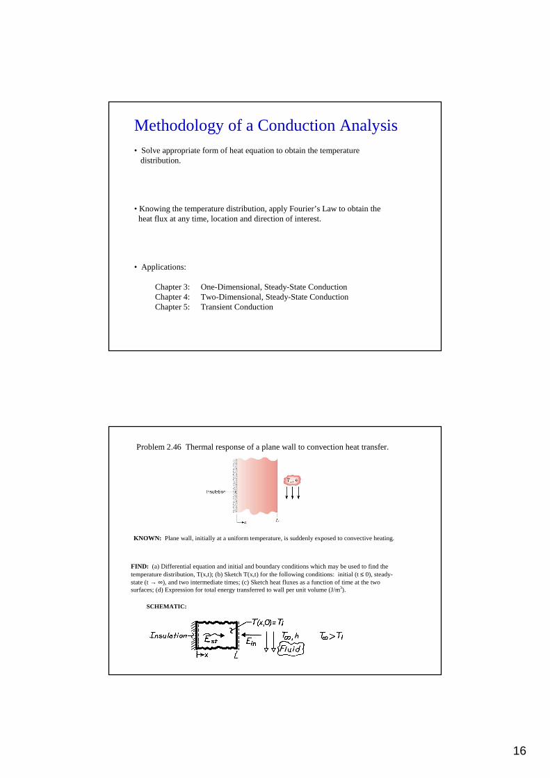
Problem 2.46 Thermal response of a plane wall to convection heat transfer.

KNOWN: Plane wall, initially at a uniform temperature, is suddenly exposed to convective heating.

FIND: (a) Differential equation and initial and boundary conditions which may be used to find the temperature distribution, T(x,t); (b) Sketch T(x,t) for the following conditions: initial (t ≤ 0), steady-state (t → ∞), and two intermediate times; (c) Sketch heat fluxes as a function of time at the two surfaces; (d) Expression for total energy transferred to wall per unit volume (J/m3).

SCHEMATIC:

17

ASSUMPTIONS: (1) One-dimensional conduction, (2) Constant properties, (3) No internal heat generation.

ANALYSIS: (a) For one-dimensional conduction with constant properties, the heat equation has the form,

2

2

T 1 T t x

∂ ∂α ∂∂

=

( ) i

0

L

Initial, t 0 : T x,0 T uniform temperature

Boundaries: x=0 T/ x) 0 adiabatic surface

x=L k T/ x) = h T

∂ ∂∂ ∂

≤ ==

− ( )L,t T surface convection∞

−

and the conditions are:

(b) The temperature distributions are shown on the sketch.

Note that the gradient at x = 0 is always zero, since this boundary is adiabatic. Note also that the gradient at x = L decreases with time.

Dividing both sides by AsL, the energy transferred per unit volume is

c) The heat flux, as a function of time, is shown on the sketch for the surfaces x = 0 and

x = L.

( )txqx ,′′

( )( )in s 0E hA T T L,t dt

∞∞= −∫

d) The total energy transferred to the wall may be expressed asd) The total energy transferred to the wall may be expressed as

in conv s0E q A dt

∞′′= ∫

( ) 3in0

E hT T L,t dt J/m

V L

∞∞ = − ∫

18

Problem 2.28 Surface heat fluxes, heat generation and total rate of radiationabsorption in an irradiated semi-transparent material with a prescribed temperature distribution.

KNOWN: Temperature distribution in a semi-transparent medium subjected to radiative flux

Problem: NonProblem: Non--uniform Generation due uniform Generation due to Radiation Absorptionto Radiation Absorption

SCHEMATIC :

FIND: (a) Expressions for the heat flux at the front and rear surfaces, (b) The heat generation rate ( )q x ,& and (c) Expression for absorbed radiation per unit surface area.

Problem : NonProblem : Non--uniform uniform Generation (Cont.)Generation (Cont.)

ASSUMPTIONS: (1) Steady-state conditions, (2) One-dimensional conduction in medium, (3) Constant properties, (4) All laser irradiation is absorbed and can be characterized by an internal

volumetric heat generation term ( )q x .&

ANALYSIS: (a) Knowing the temperature distribution, the surface heat fluxes are found using Fourier’s law,

( ) -axx 2

dT Aq k k - a e B

dx ka

′′ = − = − − +

Front Surface, x=0: ( )xA A

q 0 k + 1 B kBka a

′′ = − ⋅ + = − + <

Rear Surface, x=L: ( ) -aL -aLx

A Aq L k + e B e kB .

ka a ′′ = − + = − +

<

(b) The heat diffusion equation for the medium is

d dT q d dT

0 or q=-kdx dx k dx dx

+ =

&&

( ) -ax -axd Aq x k e B Ae .

dx ka = − + + =

&

( c ) Performing an energy balance on the medium, in out gE E E 0− + =& & &

19

Problem : NonProblem : Non--uniform uniform Generation (Cont.)Generation (Cont.)

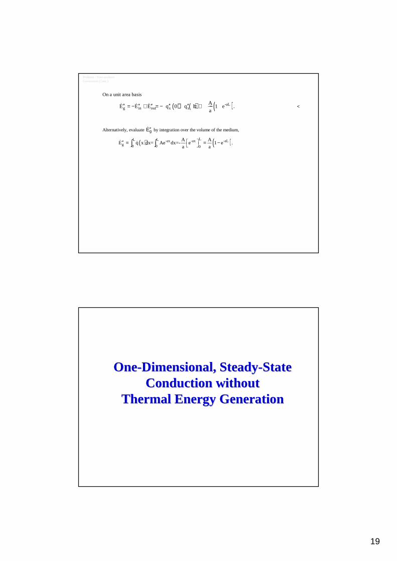
Alternatively, evaluate gE′′& by integration over the volume of the medium,

( ) ( )LL L -ax -ax -aLg 0 0 0

A AE q x dx= Ae dx=- e 1 e .

a a ′′ = = − ∫ ∫& &

On a unit area basis

( ) ( ) ( )-aLg in out x x

AE E E q 0 q L 1 e .

a′′ ′′ ′′ ′′ ′′= − + = − + = + −& & & <

OneOne--Dimensional, SteadyDimensional, Steady--StateStateConduction withoutConduction without

Thermal Energy GenerationThermal Energy Generation

20

•• Specify appropriate form of the Specify appropriate form of the heat equation.heat equation.

•• Solve for theSolve for thetemperature distributiontemperature distribution..

•• Apply Apply FourierFourier’’ s Laws Lawto determine theto determine theheat flux.heat flux.

Simplest Case:Simplest Case:OneOne--Dimensional, SteadyDimensional, Steady--StateStateConduction withConduction withNoNo Thermal EnergyThermal EnergyGenerationGeneration

•• Alternative conduction analysisAlternative conduction analysis

•• Common Geometries:Common Geometries:

–– The The Plane Wall:Plane Wall:Described in rectangular (Described in rectangular (xx) coordinate. Area ) coordinate. Area

perpendicular to direction of heat transfer is constant (inperpendicular to direction of heat transfer is constant (independent of dependent of xx).).

–– The The Tube WallTube Wall: Radial conduction through tube wall.: Radial conduction through tube wall.

–– The The Spherical Shell:Spherical Shell:Radial conduction through shell wall.Radial conduction through shell wall.

Methodology of a Conduction Analysis

•• Consider a plane wall between two fluids of different temperaturConsider a plane wall between two fluids of different temperature:e:

The Plane Wall

• Implications:

0d dT

kdx dx =

• Heat Equation:

( )Heat flux is independent of .xq x′′

( )Heat rate is independent of .xq x

• Boundary Conditions: ( ) ( ),1 ,20 , s sT T T L T= =

• Temperature Distributionfor Constant :

( ) ( ),1 ,2 ,1s s sx

T x T T TL

= + −

k

21

•• Heat Flux and Heat Rate:Heat Flux and Heat Rate:

( ),1 ,2x s sdT k

q k T Tdx L

′′ = − = −

( ),1 ,2x s sdT kA

q kA T Tdx L

= − = −

• Thermal Resistances and Thermal Circuits:tT

Rq

∆=

Conduction in a plane wall: ,t condL

RkA

=

Convection: ,1

t convRhA

=

Thermal circuit for plane wall with adjoining fluids:

1 2

1 1tot

LR

h A kA h A= + +

,1 ,2x

tot

T Tq

R∞ ∞−

=

•• Thermal Resistance for Thermal Resistance for Unit Surface Area:Unit Surface Area:

,t condL

Rk

′′ = ,1

t convRh

′′ =

Units: W/KtR ↔ 2m K/WtR′′ ↔ ⋅

• Radiation Resistance:

,1

t radr

Rh A

= ,1

t radr

Rh

′′ =

( )( )2 2r s sur s surh T T T Tεσ= + +

• Contact Resistance:

,A B

tcx

T TR

q

−′′ =′′

′′= t c

t cc

RR

A

,,

Values depend on: Materials A and B, surface finishes, interstitial conditions, and contact pressure (Tables 3.1 and 3.2)

22

•• Composite WallComposite Wallwithwith Negligible Contact Resistance:Negligible Contact Resistance:

,1 ,4x

tot

T Tq

R∞ ∞−

=

1 4

1 1 1C totA Btot

A B C

L RL LR

A h k k k h A

′′= + + + + =

• Overall Heat Transfer Coefficient (U) :

A modified form of Newton’s Law of Cooling to encompass multiple resistances to heat transfer.

x overallq UA T= ∆

1totR

UA=

•• Series Series –– Parallel Composite Wall:Parallel Composite Wall:

• Note departure from one-dimensional conditions for .F Gk k≠

• Circuits based on assumption of isothermal surfaces normal to x direction or adiabatic surfaces parallel tox direction provide approximations for .xq

23

ALTERNATIVE CONDUCTION ANALYSIS:

• STEADY STATE

• NO HEAT GENERATION

• NO HEAT LOSS FROM THE SIDES

• A(x) and k(T)

dxxx qq +=IS TEMPERATURE DISTRIBUTION ONE-DIMENSIONAL?

IS IT REASONABLE TO ASSUME ONE-DIMENSIONAL TEMPERATURE DISTRIBUTION IN x?

FROM THE FOURIER’S LAW:

dx

dTTkxAqx )()(−=

∫∫ −=T

T

x

x dTTkxA

dxq

00

)()(

Tube WallTube Wall

•• Heat Equation:Heat Equation:

The Tube Wall

10

d dTkr

r dr dr =

Is the foregoing conclusion consistent with the energy conservation requirement?

How does vary with ?rq′′ r

What does the form of the heat equation tell us about the variation of with

in the wall? rq

r

• Temperature Distributionfor Constant :k

( ) ( ),1 ,2

,21 2 2

lnln /s s

sT T r

T r Tr r r

−= +

24

•• Heat Flux Heat Flux andandHeat Rate:Heat Rate:

( ) ( )

( ) ( )

( ) ( )

,1 ,22 1

,1 ,22 1

,1 ,22 1

ln /

22

ln /

22

ln /

r s s

r r s s

r r s s

dT kq k T T

dr r r r

kq rq T T

r r

Lkq rLq T T

r r

ππ

ππ=

′′ = − = −

′ ′′= = −

′′ = − (3.27)

• Conduction Resistance:( )

( )

2 1,

2 1,

ln /Units K/W

2ln /

Units m K/W2

t cond

t cond

r rR

Lkr r

Rk

π

π

= ↔

′ = ↔ ⋅

Why is it inappropriate to base the thermal resistance on a unit surface area?

•• Composite Wall with Composite Wall with Negligible Contact Negligible Contact ResistanceResistance

( ),1 ,4,1 ,4r

tot

T Tq UA T T

R∞ ∞

∞ ∞−

= = −

1

Note that

is a constant independent of radius.totUA R −=

But, U itself is tied to specification of an interface.

( ) 1i i totU A R

−=

25

•• Heat EquationHeat Equation

Spherical Shell

22

10

d dTr

dr drr

=

What does the form of the heat equation tell us about the variation ofwith ? Is this result consistent with conservation of energy?rq r

How does vary with ? rq′′ r

• Temperature Distribution for Constant :k

( ) ( ) ( )( )

1/,1 ,1 ,2

1 2

1

1 /s s s

r rT r T T T

r r

−= − −

−

•• Heat flux, Heat Rate Heat flux, Heat Rate andandThermal Resistance:Thermal Resistance:

( ) ( ) ( ),1 ,221 21/ 1/

r s sdT k

q k T Tdr r r r

′′ = − = − −

( ) ( ) ( )2,1 ,2

1 2

44

1/ 1/r r s sk

q r q T Tr r

ππ ′′= = −−

• Composite Shell:

overallr overall

tot

Tq UA T

R

∆= = ∆

1 ConstanttotUA R −= ↔

( ) 1 Depends on i i tot iU A R A

−= ↔

( ) ( )1 2,

1/ 1/

4t condr r

Rkπ

−=

26

Critical radius (cylindrical geometry)Critical radius (cylindrical geometry)Isolamento

r1 r

T ,h¥,1 1

T ,h¥

r2

h1Lr1p2

1

T¥

T¥,1

hLrp2

1

Lk

rr 2

p2

/ln ( )

Lk1

r2

p2

/ln ( )r1

(a)

(b)

( )hLrπLkπ

rr

hLrπ

TTq revestsemr

21

12

11

1,.,

2

1

2

ln

2

1 ++

−= ∞∞

( ) ( )hLrπLkπ

rr

Lkπ

rr

hLrπ

TTq revestcomr

2

1

2

ln

2

ln

2

1 2

1

12

11

1,.,

+++

−= ∞∞

2

1

2

11

2

1

rhLrLkrd

Rd tot

ππ−=

⇒

h

krcrit =0=

rd

Rd tot ⇒ 02

2

11

2

1322

2

>

+

−=

== hkrhkr

tot

rhLrLkrd

Rd

ππ

Problem 3.23: Assessment of thermal barrier coating (TBC) for protectionof turbine blades. Determine maximum blade temperaturewith and without TBC.

Schematic:

ASSUMPTIONS: (1) One-dimensional, steady-state conduction in a composite plane wall, (2) Constant properties, (3) Negligible radiation

27

ANALYSIS: For a unit area, the total thermal resistance with the TBC is

( ) ( )1 1tot,w o t,c iZr InR h L k R L k h− −′′ ′′= + + + +

( )3 4 4 4 3 2 3 2tot,wR 10 3.85 10 10 2 10 2 10 m K W 3.69 10 m K W− − − − − −′′ = + × + + × + × ⋅ = × ⋅

With a heat flux of

,o ,i 5 2w 3 2tot,w

T T 1300Kq 3.52 10 W m

R 3.69 10 m K W

∞ ∞−

−′′ = = = ×

′′ × ⋅

the inner and outer surface temperatures of the Inconel are

( )s,i(w) ,i w iT T q h∞ ′′= + ( )5 2 2400K 3.52 10 W m 500 W m K 1104K= + × ⋅ =

( ) ( )3 4 2 5 2400 K 2 10 2 10 m K W 3.52 10 W m 1174 K− −= + × + × ⋅ × =( ) ( )s,o(w) ,i i wInT T 1 h L k q∞ ′′= + +

Without the TBC,

( )1 1 3 2tot, wo o iInR h L k h 3.20 10 m K W

− − −′′ = + + = × ⋅

( )wo ,o ,i tot,woq T T R∞ ∞′′ ′′= − = 4.06×105 W/m2 ( )wo ,o ,i tot,woq T T R∞ ∞′′ ′′= − = 4.06×105 W/m2

The inner and outer surface temperatures of the Inconel are then

( )s,i(wo) ,i wo iT T q h 1212 K∞ ′′= + =

( ) ( )[ ]s,o(wo) , i i woInT T 1 h L k q 1293 K∞ ′′= + + =

Use of the TBC facilitates operation of the Inconel below Tmax = 1250 K.

COMMENTS: Since the durability of the TBC decreases with increasing temperature, which increases with increasing thickness, limits to its thickness are associated with reliability considerations.

28

Problem 3.62: Suitability of a composite spherical shell for storingradioactive wastes in oceanic waters.

SCHEMATIC:

ASSUMPTIONS: (1) One-dimensional conduction, (2) Steady-state conditions, (3) Constant properties at 300K, (4) Negligible contact resistance.

PROPERTIES: Table A-1, Lead: k = 35.3 W/m⋅K, MP = 601K; St.St.: 15.1 W/m⋅K.

ANALYSIS: From the thermal circuit, it follows that

311

tot

T T 4q= q r

R 3∞− =

& π

The thermal resistances are:

( )Pb1 1

R 1/ 4 35.3 W/m K 0.00150 K/W0.25m 0.30m

= × ⋅ − = π

( )St.St.1 1

R 1/ 4 15.1 W/m K 0.000567 K/W0.30m 0.31m

= × ⋅ − = π

( )2 2 2convR 1/ 4 0.31 m 500 W/m K 0.00166 K/W = × × ⋅ =

π

totR 0.00372 K/W.=

The heat rate is then

( ) ( )35 3q=5 10 W/m 4 / 3 0.25m 32,725 W× =π

and the inner surface temperature is ( )1 totT T R q=283K+0.00372K/W 32,725 W∞= + 405 K < MP = 601K.=

Hence, from the thermal standpoint, the proposal is adequate.

COMMENTS: In fabrication, attention should be given to maintaining a good thermal contact. A protective outer coating should be applied to prevent long term corrosion of the stainless steel.

29

OneOne--Dimensional, SteadyDimensional, Steady--State State Conduction with Conduction with

Thermal Energy GenerationThermal Energy Generation

Implications of Energy Generation

• Involves a local (volumetric) sourceof thermal energy due to conversionfrom another form of energy in a conducting medium.

• The source may be uniformly distributed, as in the conversion fromelectrical to thermal energy(Ohmic heating):

or it may benon-uniformly distributed, as in theabsorption of radiationpassing through a semi-transparent medium.

• Generation affects the temperature distribution in the medium and causesthe heat rate to vary with location, thereby precluding inclusion of the medium in a thermal circuit.

For a plane wall,

V

RI

V

Eq

g2

==&

&

( )xq α−∝ exp&

30

The Plane Wall

• Consider one-dimensional, steady-stateconductionin aplane wallof constant k, uniform generation,and asymmetric surface conditions:

• Heat Equation:

Is the heat flux independent of x? q′′

• General Solution:

What is the form of the temperature distribution for

0?q =•

> 0?q•

< 0?q•

How does the temperature distribution change with increasing ? q•

2

20 0

d dT d T qk q

dx dx dx k + = → + =

•

•

(3.39)2

20 0

d dT d T qk q

dx dx dx k + = → + =

•

•

(3.39)

( ) 2

1 2/ 2T x q k x C x C = − + +

•

Symmetric Surface Conditions or One Surface Insulated:

• What is the temperature gradientat the centerline or the insulatedsurface?

• Why does the magnitude of the temperaturegradient increase with increasing x?

• Temperature Distribution:

Overall energy balanceon the wall →

• How do we determine the heat rate at x = L?

• How do we determine ?sT

( )2 2

21

2 s

q L xT x T

k L

= − +

•

(3.42)( )2 2

21

2 s

q L xT x T

k L

= − +

•

(3.42)

0out gE E− + =• •

( ) 0s s s

s

hA T T q A L

q LT T

h

∞

∞

− − + =

= +

•

•

(3.46)

( ) 0s s s

s

hA T T q A L

q LT T

h

∞

∞

− − + =

= +

•

•

(3.46)

31

Radial SystemsCylindrical (Tube) Wall Spherical Wall (Shell)

Solid Cylinder (Circular Rod) Solid Sphere

• Heat Equations:Cylindrical

10

d dTkr q

r dr dr

• + =

Spherical

2

2

10

d dTkr q

r dr dr

• + =

• Heat Equations:Cylindrical

10

d dTkr q

r dr dr

• + =

Spherical

2

2

10

d dTkr q

r dr dr

• + =

Temperature Distribution Surface Temperature

Overall energy balance:

Or from asurface energy balance:

• Solution forUniform Generationin a Solid Sphere of Constant kwith Convection Cooling:

• A summary of temperature distributions is provided in Appendix Cfor plane, cylindrical and spherical walls, as well as for solidcylinders and spheres. Note how boundary conditions are specifiedand how they are used to obtain surface temperatures.

32

13

dT q rkr C

dr= − +

•

2

126

Cq rT C

k r= − − +

•

0 10 0rdT

Cdr = = → =|

( )2

2 6o

o s s

q rT r T C T

k= → = +

•

( )2 2

21

6o

s

o

q r rT r T

k r

= − +

•

0out gE E− + =• •

3o

s

q rT T

h∞→ = +•

0 in outE E− =• • ( )cond o convq r q→ =

3o

s

q rT T

h∞→ = +•

32

Problem 3.91 Thermal conditions in a gas-cooled nuclear reactorwith a tubular thorium fuel rod and a concentric graphite sheath: (a) Assessment of thermal integrityfor a generation rate of . (b) Evaluation oftemperature distributions in the thorium and graphitefor generation rates in the range .

8 310 W/mq =�

8 810 5x10q≤ ≤•

Problem 3.91 Thermal conditions in a gas-cooled nuclear reactorwith a tubular thorium fuel rod and a concentric graphite sheath: (a) Assessment of thermal integrityfor a generation rate of . (b) Evaluation oftemperature distributions in the thorium and graphitefor generation rates in the range .

8 310 W/mq =�

8 810 5x10q≤ ≤•

Schematic:Schematic:

Assumptions: (1) Steady-state conditions, (2) One-dimensional conduction, (3) Constant properties, (4) Negligible contact resistance, (5) Negligible radiation, (6) Adiabatic surface at r1.

Properties: Table A.1, Thorium: 2000 ; Table A.2, Graphite: 2300 .mp mpT K T K≈ ≈Properties: Table A.1, Thorium: 2000 ; Table A.2, Graphite: 2300 .mp mpT K T K≈ ≈

Analysis: (a) The outer surface temperature of the fuel, T2 , may be determined from the rate equation

2

tot

T Tq

R∞−′ =

′

where( )3 2

3

1n / 10.0185 m K/W

2 2totg

r rR

k r hπ π′ = + = ⋅

The heat rate may be determined by applying an energy balance to a control surface about the fuel element,

out gE E=• •

or, per unit length,out gE E′ ′=

• •

Since the interior surface of the element is essentially adiabatic, it follows that

Hence,

With zero heat flux at the inner surface of the fuel element, Eq. C.14 yields

( )2 2

2 1 17,907 W/mq q r rπ′ = − =•

( )2 17,907 W/m 0.0185 m K/W 600 931totT q R T K K∞′ ′= + = + =�

2

2 2 2

2 1 11 2 2

2 1

1 1n 931 25 18 938 <4 2t t

rq r r q rT T K K K K

k r k r

= + − − = + − =

• •

33

Since T1 and T2 are well below the melting points of thorium and graphite, the prescribedoperating condition is acceptable.

(b) The solution for the temperature distribution in a cylindrical wall with generation is

( )2 2

22 2

2

14t

t

q r rT r T

k r

= + −

•

( ) ( )( )

2

2 1

2 21n /2 1

2 12 1n /2

14

r r

r rt

q r rT T

k r

− − + −

•

(C.2)( ) ( )( )

2

2 1

2 21n /2 1

2 12 1n /2

14

r r

r rt

q r rT T

k r

− − + −

•

(C.2)

Boundary conditions at r1 and r2 are used to determine T1 and T 2 .

( )

( )

2 2

2 12 12

21

1 1

1 2 1

14

: 02 1n /

t

q r rk T T

k rqrr r q

r r r

− + − ′′= = = −

•

•(C.14)( )

( )

2 2

2 12 12

21

1 1

1 2 1

14

: 02 1n /

t

q r rk T T

k rqrr r q

r r r

− + − ′′= = = −

•

•(C.14)

( )( )

( )

2 2

2 12 12

22

2 2 2

2 2 1

14

:2 1n /

t

qr rk T T

k rq rr r U T T

r r r∞

− + − = − = −

•

•

(C.17)

( )( )

( )

2 2

2 12 12

22

2 2 2

2 2 1

14

:2 1n /

t

qr rk T T

k rq rr r U T T

r r r∞

− + − = − = −

•

•

(C.17)

( ) ( )1 12 2 22tot totU A R r Rπ− −′ ′ ′= = (3.32)( ) ( )1 12 2 22tot totU A R r Rπ− −′ ′ ′= = (3.32)

0.008 0.009 0.01 0.011

Radial location in fuel, r(m)

500

900

1300

1700

2100

2500

Tem

pera

ture

, T(K

)

qdot = 5E8qdot = 3E8qdot = 1E8

The following results are obtained for temperature distributions in the graphite.

Operation at is clearly unacceptable since the melting point of

thorium would be exceeded. To prevent softening of the material, which would occur

below the melting point, the reactor should not be operated much above .

The small radial temperature gradients are attributable to the large value of .

8 35x10 W/mq =•

tk

8 33x10 W/mq =•

Operation at is clearly unacceptable since the melting point of

thorium would be exceeded. To prevent softening of the material, which would occur

below the melting point, the reactor should not be operated much above .

The small radial temperature gradients are attributable to the large value of .

8 35x10 W/mq =•

tk

8 33x10 W/mq =•

34

0.011 0.012 0.013 0.014

Radial location in graphite, r(m)

500

900

1300

1700

2100

2500

Tem

pera

ture

, T(K

)

qdot = 5E8qdot = 3E8qdot = 1E8

the temperature distribution in the graphite is

Using the value of T2 from the foregoing solution and computing T3 from the surface condition,

( )( )

2 3

3 2

2

1n /gk T T

qr r

π −′ = (3.27)

( )( )

2 3

3 2

2

1n /gk T T

qr r

π −′ = (3.27)

( ) ( )2 3

32 3 3

1n1n /g

T T rT r T

r r r

−= +

(3.26)( ) ( )2 3

32 3 3

1n1n /g

T T rT r T

r r r

−= +

(3.26)

Operation at is problematic for the graphite. Larger temperature gradientsare due to the small value of .

8 35x10 W/mq =•

gkOperation at is problematic for the graphite. Larger temperature gradientsare due to the small value of .

8 35x10 W/mq =•

gk

Comments: (i) What effect would a contact resistance at the thorium/graphite interface have on

temperatures in the fuel element and on the maximum allowable value of ? q•

What would be the influence of such

effect on temperatures in the fuel element and the maximum allowable value of ?q•

(ii) Referring

to the schematic, where might radiation effects be significant?









(ii) Referring

to the schematic, where might radiation effects be significant?

35

Extended SurfacesExtended Surfaces

36

Nature and Rationale of Extended Surfaces• An extended surface (also know as a combined conduction-convection system

or afin) is a solid within whichheat transfer by conductionis assumedto be one dimensional, while heat is also transferred byconvection(and/orradiation) from the surface in a direction transverse to that of conduction.

– Why is heat transfer by conduction in the x-direction not, in fact, one-dimensional?

– If heat is transferred from the surface to the fluid by convection, what surface condition is dictated by the conservation of energy requirement?

– What is the actual functional dependence of the temperature distribution inthe solid?

– If the temperature distribution is assumed to be one-dimensional, that is,T=T(x) , how should the value of T be interpreted for any x location?

– How does vary with x ?,cond xq

– When may the assumption of one-dimensional conduction be viewed as anexcellent approximation? Thethin-fin approximation.

as for a gas and natural convection.

• Extended surfaces may exist in many situations but are commonly used asfins to enhance heat transfer by increasing the surface areaavailable forconvection (and/or radiation). They are particularly beneficial when is small,h

• Some typical fin configurations:

Straight finsof (a) uniform and (b) non-uniform cross sections; (c) annularfin, and (d)pin fin of non-uniform cross section.

37

(a) (b) (c)

(d) (e) (f)

(g) (h) (i)

TYPICAL FIN CONFIGURATIONS

z

x

y

dx

x

Ac (x)

dqconv

qx

dAs

qx+dx

convdxxx qdqq += +

xd

TdAkq cx −=

( )∞−= TTdAhqd sconv

dxxd

TdA

xd

dk

xd

TdAkdx

xd

qdqq cc

xxdxx

−−=+=+

( ) 0=−+

− ∞TT

xd

Adh

xd

TdA

xd

dk s

c

( ) 011

2

2

=−

−

+ ∞TT

xd

Ad

k

h

Axd

Td

xd

Ad

Axd

Td s

c

c

c

The Fin Equation

38

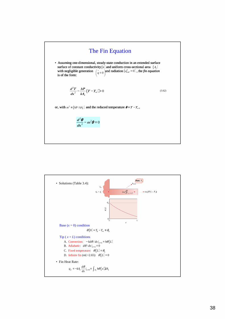
The Fin Equation

22

20− =d

mdx

θθθθ θθθθ

( )2

20∞− − =

c

d T hPT T

kAdx(3.62)( )

2

20∞− − =

c

d T hPT T

kAdx(3.62)

• Assuming one-dimensional, steady-state conduction in an extended surfacesurface of constant conductivity and uniform cross-sectional area , with negligible generation and radiation , the fin equationis of the form:

( )k ( )cA

0q =

• ( )0radq′′ =

• Assuming one-dimensional, steady-state conduction in an extended surfacesurface of constant conductivity and uniform cross-sectional area , with negligible generation and radiation , the fin equationis of the form:

( )k ( )cA

0q =

• ( )0radq′′ =

or, with and the reduced temperature ,( )2 / cm hP kA≡ ∞≡ −T Tθθθθor, with and the reduced temperature ,( )2 / cm hP kA≡ ∞≡ −T Tθθθθ

• Solutions (Table 3.4):

Base (x = 0) condition

( )0 b bT Tθ θ∞= − ≡

Tip ( x = L) conditions

( )A. : Conv ect /i n |o x Lkd dx h Lθ θ=− =B. : / |Adiabati 0c x Ld dxθ = =

( )Fixed temperC. : atu re LLθ θ=( )D. (Infinite fin >2.65 ): 0mL Lθ =

• Fin Heat Rate:

( )0|ff c x A s

dq kA h x dA

dx

θ θ== − = ∫

39

Caso Condição de

fronteira em x = L Distribuição de temperaturas

θ / θ b Taxa de transmissão de

calor

(i) ( )Lθhxd

θdk

Lx

=

−

=

( )[ ] ( )[ ]

( ) ( )Lmkm

hLm

xLmkm

hxLm

sinhcosh

sinhcosh

+

−+−

( ) ( )

( ) ( )Lmkm

hLm

Lmkm

hLm

Msinhcosh

coshsinh

+

+

(ii) 0=

=Lxxd

θd ( )[ ]( )Lm

xLm

cosh

cosh − ( )LmM tanh

(iii) ( ) LθLθ = ( ) ( ) ( )[ ]

( )Lm

xLmxmbL

sinh

sinhsinh −+θθ ( )( )Lm

LmM bL

sinh

/cosh θθ−

(iv) ( ) 0=Lθ xme− M

cAk

Phm =2

bc θAkPhM =

Fin Performance Parameters• Fin Efficiency:

,max

f ff

f f b

q q

q hAη

θ≡ =

How is the efficiency affected by the thermal conductivity of the fin?Expressions for are provided in Table 3.5 for common geometries.fη

( )1/ 2222 / 2fA w L t = +

( )/ 2pA t L=( )( )

1

0

21

2f

I mL

mL I mLη =

• Fin Effectiveness:

Consider a triangular fin:

,

ff

c b b

q

hAε

θ≡

• Fin Resistance: with , and /f ch k A Pε ↑ ↓ ↑ ↓

,

1bt f

f f f

Rq hA

θη

≡ =

40

Correction of fin length to account for heat loss from the tip

extremidadeisolada

Transmissão de calorna extremidade

( ) ( ) ( )LLLPhLAhq cctipf θθ −≈=,

P

ALL c

c +=

Fin of rectangular cross section with t << w:

Lc = L + t / 2

Fin of circular cross section :

Lc = L + D / 4

Approximation error negligible if ht / k or hD / 2k ≤ 0.0625

Fins efficiency

0.0 1.0 2.0 3.0 4.0 5.00.0

0.2

0.4

0.6

0.8

1.0

1.82

4

31.6

1.4

ri

L

ro

t

1=

i

o

r

rhf

0.0 1.0 2.0 3.0 4.0 5.0

1.0

0.9

0.8

0.7

0.6

0.5

0.4

0.3

0.2

0.1

0.0

(a)

(b)

(c)

(d)

(e)

hf

t

x

y (x)

41

Fin Arrays• Representative arrays of

(a) rectangular and(b) annular fins.

– Total surface area:t f bA NA A= +

Number of fins Area of exposed base (primesurface)

– Total heat rate:

,

bt f f b b b o t b

t o

q N hA hA hAR

θη θ θ η θ= + ≡ =

– Overall surface efficiencyandresistance:

,

1bt o

t o t

Rq hA

θη

= =

( )1 1fo f

t

NA

Aη η= − −

• Equivalent Thermal Circuit :

• Effect of Surface Contact Resistance:

( )( ),

bt t bo c

t o c

q hAR

θη θ= =

( )1

1 1f fo c

t

NA

A C

ηη

= − −

( )1 , ,1 /f f t c c bC hA R Aη ′′= +

( )( )

,

1t o c

to c

RhAη

=

42

Problem 3.116: Assessment of cooling scheme for gas turbine blade.Determination of whether blade temperatures are lessthan the maximum allowable value (1050 °C) for prescribed operating conditions and evaluation of bladecooling rate.

Schematic:

Assumptions: (1) One-dimensional, steady-state conduction in blade, (2) Constant k, (3)Adiabatic blade tip, (4) Negligible radiation.

Analysis: Conditions in the blade are determined by Case B of Table 3.4.

(a) With the maximum temperature existing at x=L, Eq. 3.75 yields

( )b

T L T 1

T T cosh mL∞

∞

−=

−

( ) ( )1/ 21/ 2 2 4 2cm hP/kA 250W/m K 0.11m/20W/m K 6 10 m−= = ⋅ × ⋅ × × = 47.87 m-1 ( ) ( )1/ 21/ 2 2 4 2cm hP/kA 250W/m K 0.11m/20W/m K 6 10 m−= = ⋅ × ⋅ × × = 47.87 m-1

mL = 47.87 m-1 × 0.05 m = 2.39

From Table B.1, . Hence,coshmL=5.51From Table B.1, . Hence,coshmL=5.51

( ) 1200 300 1200 5 51 1037= + − =o o oT L C ( ) C/ . C

and, subject to the assumption of an adiabatic tip, the operating conditions are acceptable.

(b) With ( ) ( ) ( )1/ 22 4 21/ 2c bM hPkA 250W/m K 0.11m 20W/m K 6 10 m 900 C 517W−= Θ = ⋅ × × ⋅ × × − = −o ,

Eq. 3.76 and Table B.1 yield

( )fq M tanh mL 517W 0.983 508W= = − = −

Hence, b fq q 508W= − =

Comments: Radiation losses from the blade surface contribute to reducing the blade temperatures, but what is the effect of assuming an adiabatic tip condition? Calculatethe tip temperature allowing for convection from the gas.

43

Problem 3.132: Determination of maximum allowable power for a 20mm x 20mm electronic chip whose temperature is not to exceed

when the chip is attached to an air-cooled heat sink with N=11 fins of prescribed dimensions.

cq

85 C,cT = o

Problem 3.132: Determination of maximum allowable power for a 20mm x 20mm electronic chip whose temperature is not to exceed

when the chip is attached to an air-cooled heat sink with N=11 fins of prescribed dimensions.

cq

85 C,cT = o

Schematic:

Assumptions: (1) Steady-state, (2) One-dimensional heat transfer, (3) Isothermal chip, (4)Negligible heat transfer from top surface of chip, (5) Negligible temperature rise for air flow,(6) Uniform convection coefficient associated with air flow through channels and over outersurface of heat sink, (7) Negligible radiation.

Analysis: (a) From the thermal circuit,

c cc

tot t,c t,b t,o

T T T Tq

R R R R∞ ∞− −

= =+ +

( )2 6 2 2t,c t,cR R / W 2 10 m K / W / 0.02m 0.005 K / W−′′= = × ⋅ =

( )2t,b bR L / k W= ( )W / m K

20.003m /180 0.02m 0.042 K / W⋅= =

From Eqs. (3.103), (3.102), and (3.99) ( )ft,o o f t f b

o t t

N A1R , 1 1 , A N A A

h A A= = − − = +η η

η

Af = 2WLf = 2 × 0.02m × 0.015m = 6 × 10-4 m2

Ab = W2 – N(tW) = (0.02m)2 – 11(0.182 × 10-3 m × 0.02m) = 3.6 × 10-4 m2

At = 6.96 × 10-3 m2

With mLf = (2h/kt)1/2 Lf = (200 W/m2⋅K/180 W/m⋅K × 0.182 × 10-3m)1/2 (0.015m) =

1.17, tanh mLf = 0.824 and Eq. (3.87) yields

ff

f

tanh mL 0.8240.704

mL 1.17= = =η

ηo = 0.719,

Rt,o = 2.00 K/W, and

( )( )c

85 20 Cq 31.8 W

0.005 0.042 2.00 K / W

− °= =

+ +

44

Comments: The heat sink significantly increases the allowable heat dissipation. If it were not used and heat was simply transferred by convection from the surface of the chip with

from Part (a) would be replaced by 2100 W/m , 2.05 K/Wtoth K R= =�21/hW 25 K/W, yielding 2.60 W.cnv cR q= = =

Transient Conduction:Transient Conduction:The Lumped Capacitance The Lumped Capacitance

MethodMethod

45

Transient Conduction• A heat transfer process for which thetemperature varies with time, as well

as location within a solid.

• It is initiated whenever a system experiences a change in operating conditionsand proceeds until a new steady state (thermal equilibrium) is achieved.

• It can be induced by changes in:– surface convection conditions ( ),,h T∞

• Solution Techniques

– The Lumped Capacitance Method– Exact Solutions– The Finite-Difference Method (not to be studied)

– surface radiation conditions ( ),,r surh T

– a surface temperature or heat flux, and/or

– internal energy generation.

The Lumped Capacitance Method

• Based on the assumptionof aspatially uniform temperature distributionthroughout the transient process.

• Why is the assumption never fully realized in practice?

• General Lumped Capacitance Analysis:

� Consider a general case, which includes convection,radiation and/or an appliedheat flux at specified surfacesas well as internal energy generation

( ), , ,, , ,s c s r s hA A A

)t(T)t,r(T ≈r

46

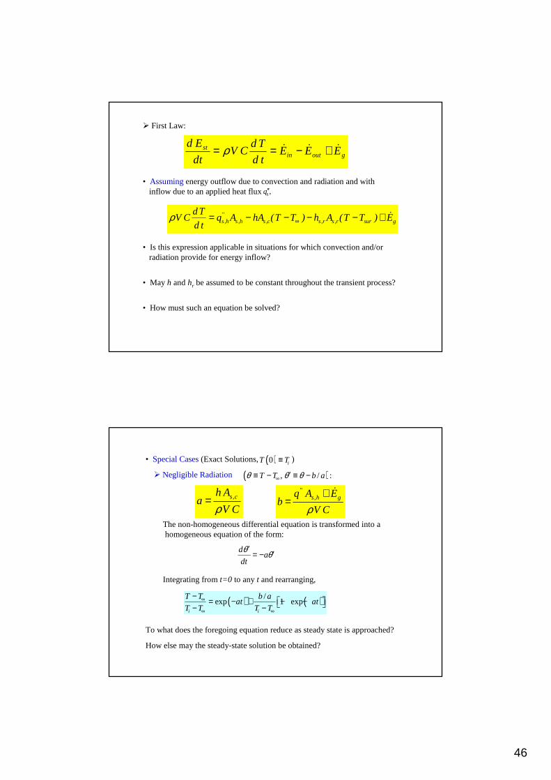
� First Law:

• Assumingenergy outflow due to convection and radiation and withinflow due to an applied heat flux ,sq′′

• Is this expression applicable in situations for which convection and/orradiation provide for energy inflow?

• May h and hr be assumed to be constant throughout the transient process?

• How must such an equation be solved?

gsurr,sr,sc,sh,s''h,s E)TT(Ah)TT(hAAq

td

TdCV &+−−−−= ∞ρ

goutin

st EEEtd

TdCV

dt

Ed &&& +−== ρ

• Special Cases(Exact Solutions, ) ( )0 iT T≡

� Negligible Radiation ( ), / :T T b aθ θ θ∞ ′≡ − ≡ −

The non-homogeneous differential equation is transformed into a homogeneous equation of the form:

da

dt

θ θ′

′= −

Integrating from t=0 to anyt and rearranging,

( ) ( )/exp 1 exp

i i

T T b aat at

T T T T∞

∞ ∞

− = − + − − − −

To what does the foregoing equation reduce as steady state is approached?

How else may the steady-state solution be obtained?

CV

Aha cs

ρ,=

CV

EAqb ghs

ρ

&+= ,

''

47

� Negligible Radiation and Source Terms , 0, 0 :gr sh h E q ′′>> = =

�

( ),s c

dTc hA T T

dtρ ∞∀ = − −

, is c

t

o

c d

hAdt

θ

θ

ρ θθ

∀ = −∫∫

,s c

i i

hAT Texp t

T T c

θθ ρ

∞

∞

−= = − − ∀ t

t

τ

= −

exp

Thethermal time constant is defined as

( ),

1t

s c

chA

τ ρ

≡ ∀

ThermalResistance, Rt

Lumped ThermalCapacitance, Ct

Thechange in thermal energy storagedue to the transient process ist

outsto

E Q E dt∆ ≡ − = −∫�

,

t

s co

hA dtθ= − ∫ ( ) 1 expit

tcρ θ

τ

= − ∀ − −

(5.8)

� Negligible Convection and Source Terms , 0, 0 :gr sh h E q ′′>> = =

�

Assuming radiation exchange with large surroundings,

( )4 4,s r sur

dTc A T T

dtρ ε σ∀ = − −

,

4 4i

s r T

surTo

tA

c

dTT T

dtε σ

ρ=

∀ −∫∫

3,

1n 1n4

sur sur i

s r sur sur sur i

T T T Tct

A T T T T T

ρε σ

+ +∀ = − − −

Result necessitates implicit evaluation of T(t).

1 12 tan tan i

sur sur

TT

T T− −

+ −

48

The Biot Number and Validity ofThe Lumped Capacitance Method

• The Biot Number: The first of manydimensionless parametersto beconsidered.

� Definition:chL

Bik

≡

convection or radiation coefficienth →

thermal conductivity of t so e dh lik →

of the solid ( / or coordinate

associated with maximum spa

char

tial temperature differe

acteristic lengt

e

h

nc )c sL A→ ∀

� Physical Interpretation:

� Criterion for Applicability of Lumped Capacitance Method:

1Bi <<

/

/

1/c s cond solid

s conv solid fluid

L kA R TBi

hA R T

∆=∆

� �= =

Problem 5.11: Charging a thermal energy storagesystem consistingof a packed bedof aluminum spheres.

KNOWN: Diameter, density, specific heat and thermal conductivity of aluminum spheres used in packed bed thermal energy storage system. Convection coefficient and inlet gas temperature.

FIND: Time required for sphere at inlet to acquire 90% of maximum possible thermal energy and the corresponding center temperature.

Schematic:Schematic:

49

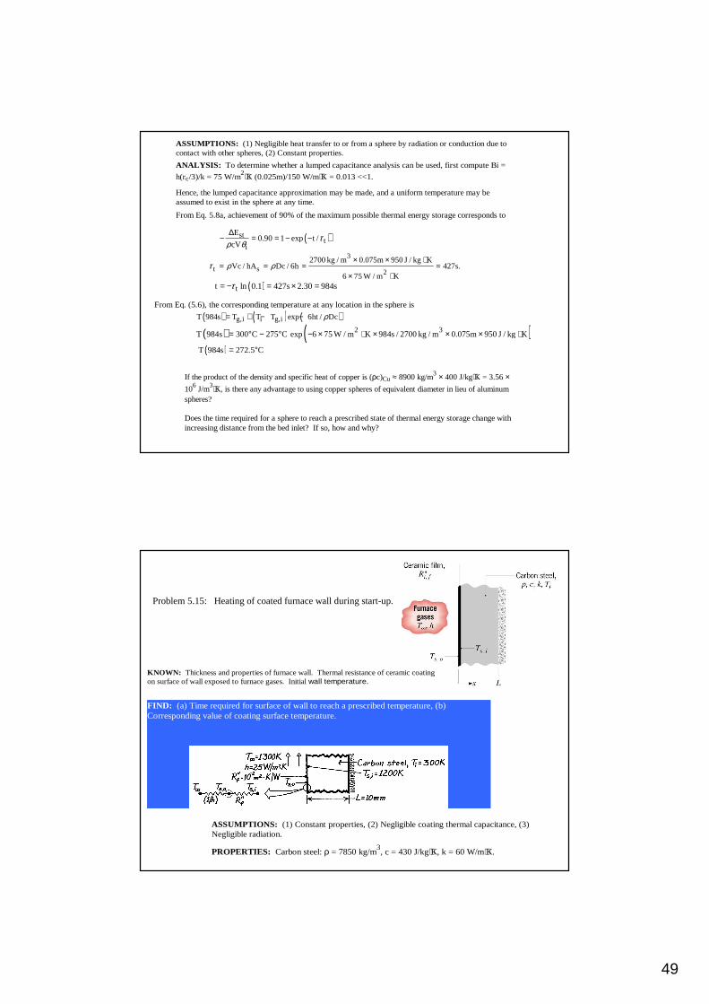
ASSUMPTIONS: (1) Negligible heat transfer to or from a sphere by radiation or conduction due to contact with other spheres, (2) Constant properties.

ANALYSIS: To determine whether a lumped capacitance analysis can be used, first compute Bi =

h(ro/3)/k = 75 W/m2⋅K (0.025m)/150 W/m⋅K = 0.013 <<1.

Hence, the lumped capacitance approximation may be made, and a uniform temperature may be assumed to exist in the sphere at any time.

From Eq. 5.8a, achievement of 90% of the maximum possible thermal energy storage corresponds to

( )stt

i

E0.90 1 exp t /

cVτ

ρ θ∆

− = = − −

( )tt ln 0.1 427s 2.30 984sτ= − = × =

3

t s 2

2700 kg / m 0.075m 950 J / kg KVc / hA Dc / 6h 427s.

6 75 W / m Kτ ρ ρ

× × ⋅= = = =

× ⋅

From Eq. (5.6), the corresponding temperature at any location in the sphere is

( ) ( ) ( )g,i i g,iT 984s T T T exp 6ht / Dcρ= + − −

( ) ( )2 3T 984s 300 C 275 C exp 6 75 W / m K 984s / 2700 kg / m 0.075m 950 J / kg K= ° − ° − × ⋅ × × × ⋅

( )T 984s 272.5 C= °

If the product of the density and specific heat of copper is (ρc)Cu ≈ 8900 kg/m3 × 400 J/kg⋅K = 3.56 ×

106 J/m3⋅K, is there any advantage to using copper spheres of equivalent diameter in lieu of aluminum spheres?

Does the time required for a sphere to reach a prescribed state of thermal energy storage change with increasing distance from the bed inlet? If so, how and why?

Problem 5.15: Heating of coated furnace wall during start-up.

KNOWN: Thickness and properties of furnace wall. Thermal resistance of ceramic coating on surface of wall exposed to furnace gases. Initial wall temperature.

FIND: (a) Time required for surface of wall to reach a prescribed temperature, (b) Corresponding value of coating surface temperature.

ASSUMPTIONS: (1) Constant properties, (2) Negligible coating thermal capacitance, (3) Negligible radiation.

PROPERTIES: Carbon steel: ρ = 7850 kg/m3, c = 430 J/kg⋅K, k = 60 W/m⋅K.

50

ANALYSIS: Heat transfer to the wall is determined by the total resistance to heat transfer from the gas to the surface of the steel, and not simply by the convection resistance.

Hence, with ( )11

1 2 2 2tot f 2

1 1U R R 10 m K/W 20 W/m K.

h 25 W/m K

−−− − ′′ ′′= = + = + ⋅ = ⋅

⋅

2UL 20 W/m K 0.01 mBi 0.0033 1

k 60 W/m K

⋅ ×= = = <<⋅

and the lumped capacitance method can be used. (a) From Eqs. (5.6) and (5.7),

( ) ( ) ( )t t ti

T Texp t/ exp t/R C exp Ut/ Lc

T Tτ ρ∞

∞

−= − = − = −

−

( )3

2i

7850 kg/m 0.01 m 430 J/kg KT TLc 1200 1300t ln ln

U T T 300 130020 W/m K

ρ ∞∞

⋅− −= − = −− −⋅

t 3886s 1.08h.= =

(b) Performing an energy balance at the outer surface (s,o),

( ) ( )s,o s,o s,i fh T T T T / R∞ ′′− = −

( ) ( )

2 -2 2s,i fs,o 2f

hT T / R 25 W/m K 1300 K 1200 K/10 m K/WT

h 1/ R 25 100 W/m K

∞ ′′+ ⋅ × + ⋅= =′′+ + ⋅

s,oT 1220 K.=

How does the coating affect the thermal time constant?

Transient Conduction:Transient Conduction:Spatial Effects and the Role ofSpatial Effects and the Role of

Analytical SolutionsAnalytical Solutions

51

Solution to the Heat Equation for a Plane Wall withSymmetrical Convection Conditions

• If the lumped capacitance approximation can not be made, consideration mustbe given to spatial, as well as temporal, variations in temperature during thetransient process.

• For a plane wall with symmetrical convectionconditions and constant properties, theheatequationandinitial/boundaryconditions are:

2

2

1T T

x tα∂ ∂=∂ ∂

( ),0 iT x T=

0

0x

T

x =

∂ =∂

( ),x L

Tk h T L t T

x ∞=

∂ − = − ∂

• Existence of seven independent variables:

( ), , , , , ,iT T x t T T k hα∞=

How may the functional dependence be simplified?

• Non-dimensionalizationof Heat Equation and Initial/Boundary Conditions:

Dimensionless temperature difference: *

i i

T T

T T

θθθ

∞

∞

−≡ =−

*x

xL

≡Dimensionless coordinate:

The Biot Number:solid

hLBi

k≡

( )* * , ,f x Fo Biθ =• Exact Solution:

( ) ( )* 2 *

1exp cosn n n

nC Fo xθ ζ ζ

∞

== −∑

( )4sin

tan2 sin 2

nn n n

n n

C Biζ ζ ζ

ζ ζ= =

+

See Appendix B.3 for first four roots (eigenvalues ) of Eq. (5.39c)1 4,...,ζ ζ

Dimensionless time:*2

tt Fo

L

α≡ ≡

Fourierthe NumberFo →

52

• TheOne-Term Approximation :( )0.2Fo >

� Variation of midplane temperature (x*= 0) with time : ( )Fo

( )( ) ( )* 2

1 1expoo

i

T TC Fo

T Tθ ζ∞

∞

−≡ ≈ −

−

1 1Table 5.1 and as a function of C Biζ→

( )Fo� Variation of temperature with location (x*) and time :

( )* * *1coso xθ θ ζ=

� Change in thermal energy storage with time:

stE Q∆ = −

1 *

1

sin1o oQ Q

ζ θζ

= −

( )o iQ c T Tρ ∞= ∀ −

Can the foregoing results be used for a plane wall that is well insulated on oneside and convectively heated or cooled on the other?

Can the foregoing results be used if an isothermal condition is instantaneously imposed on both surfaces of a plane wall or on one surface ofa wall whose other surface is well insulated?

( )s iT T≠

-------------------------------------------------

1.130301.111181.103810.897831.064190.624440.45

1.116351.052791.093140.851581.058040.593240.40

1.102260.989661.082260.801401.051660.559220.35

1.088020.920791.071160.746461.045050.521790.30

1.073650.844731.059840.685591.038190.480090.25

1.059150.759311.048300.616971.031090.432840.20

1.044530.660861.036550.537611.023720.377880.15

1.029800.542281.024580.441681.016090.311050.10

1.026840.514971.022160.419541.014540.295570.09

1.023870.486001.019730.396031.012970.279130.08

1.020900.455061.017290.370921.011380.261530.07

1.017930.421731.014850.343831.009790.242530.06

1.014950.385371.012400.314261.008190.221760.05

1.011970.345031.009930.281431.006570.198680.04

1.008980.299101.007460.244031.004950.172340.03

1.005990.244461.004980.199501.003310.140950.02

1.003000.173031.002500.141241.001660.099830.01

c1ζ1c1ζ1c1ζ1

EsferaCilindro longoPlaca plana

Bi

53

Graphical Representation of the One-Term ApproximationThe Heisler Charts – Plane wall

• Midplane Temperature:


• Change in Thermal Energy Storage:

54

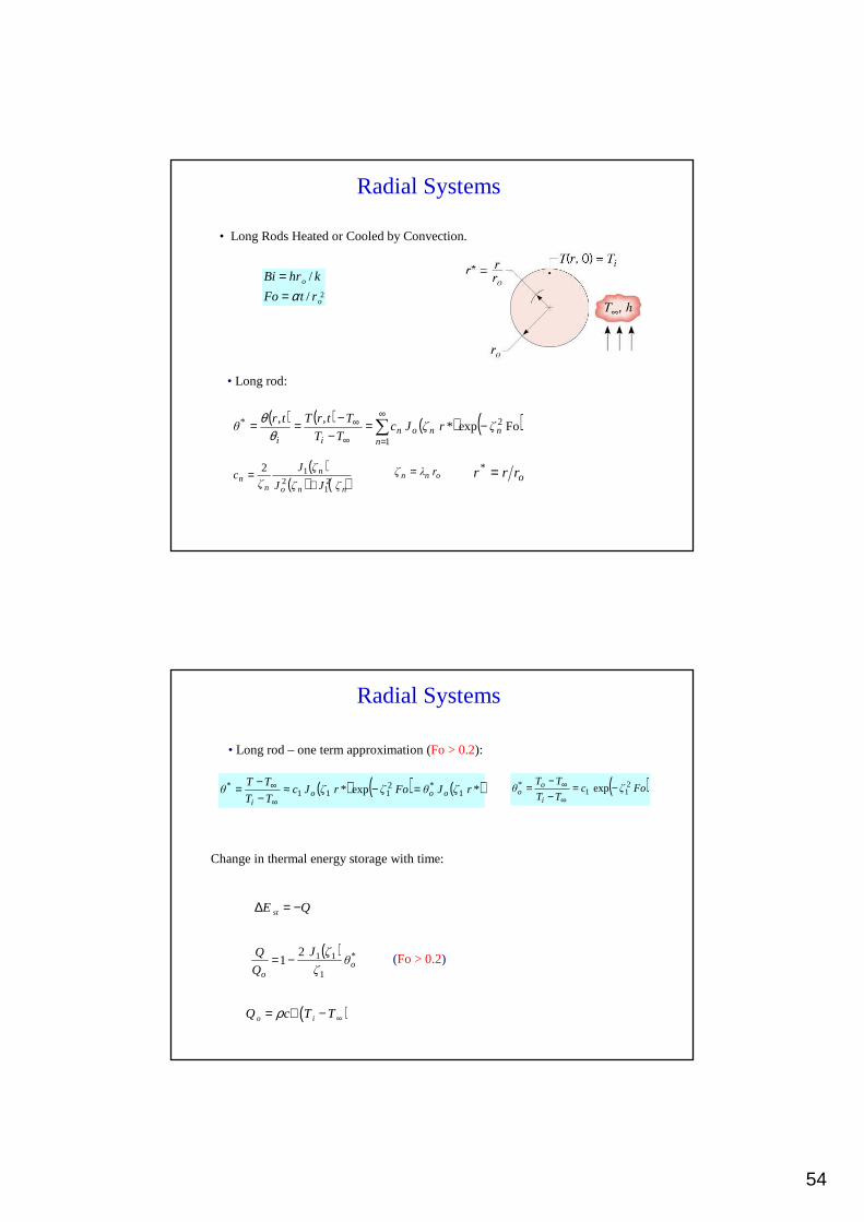
Radial Systems

• Long Rods Heated or Cooled by Convection.

2

/

/o

o

Bi hr k

Fo t rα==

( ) ( ) ( ) ( )∑∞

=∞

∞ −=−

−==1

2 Foexp*,,

nnnon

ii

* ζrζJcTT

TtrTtrθ

θθ

( )( ) ( )nno

n

nn

ζJζJ

ζJ

ζc

21

212

+=

(5.184a)

onn rλζ =

• Long rod:

orrr =*

Radial Systems

(5.184a)

( ) *o

o

θζ

ζJ

Q

Q

1

1121−=

Change in thermal energy storage with time:

stE Q∆ = −

( )o iQ c T Tρ ∞= ∀ −

(Fo > 0.2)

( ) ( ) ( )*exp* 12111 rζJθFoζrζJc

TT

TTθ o

*oo

i

* =−≈−−=

∞

∞ ( )FoζcTT

TTθ

i

o*o

211 exp−=

−−

=∞

∞

• Long rod – one term approximation (Fo > 0.2):

55

Graphical Representation of the One-Term ApproximationThe Heisler Charts – Infinite cylinder

• Centerline Temperature:



56

Spherical Systems• Spheres Heated or Cooled by Convection.

2

/

/o

o

Bi hr k

Fo t rα==

(5.184a)• Sphere:

orrr =*

( ) ( ) ( ) ( )∑∞

=∞

∞ −=−

−==

1

2 *sin*

1Foexp

,,

nn

nnn

ii

* rζrζ

ζcTT

TtrTtrθ

θθ

( )( )nn

nnnn

ζζ

ζζζc

2sin2

cossin4

−−

=

Bitanco1 =− nn ζζ

Spherical Systems

(5.184a)

Change in thermal energy storage with time:

stE Q∆ = −

( )o iQ c T Tρ ∞= ∀ −

(Fo > 0.2)

( )FoζcTT

TTθ

i

o*o

211 exp−=

−−

=∞

∞

• Sphere – one term approximation (Fo > 0.2):

( ) ( ) ( )*

*sinFoexp

*

*sin

1

121

1

11 rζ

rζθζ

rζ

rζc

TT

TTθ *

oi

* =−≈−−=

∞

∞

( )11131

cossin3

1 ζζζζ

θ

Q

Q *o

o

−−=

57

Graphical Representation of the One-Term ApproximationThe Heisler Charts – Sphere

• Center Temperature:



58

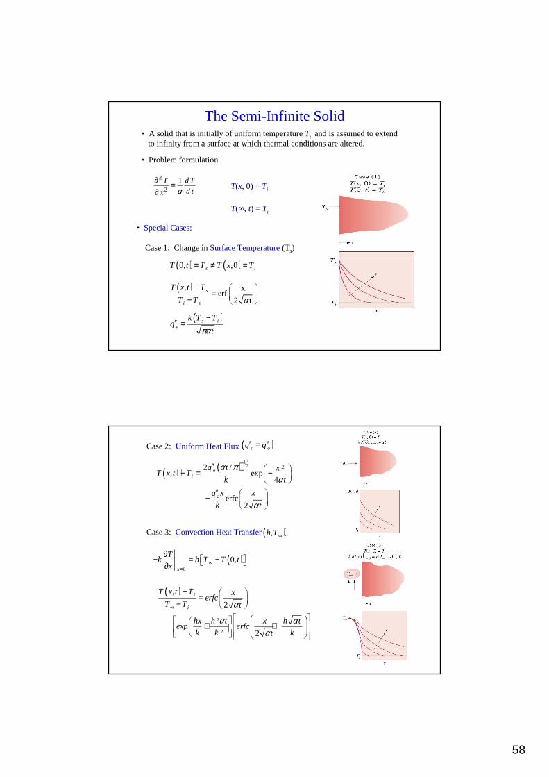
The Semi-Infinite Solid• A solid that is initially of uniform temperature Ti and is assumed to extend

to infinity from a surface at which thermal conditions are altered.

• Special Cases:

Case 1: Change inSurface Temperature(Ts)

( ) ( )0, ,0s iT t T T x T= ≠ =

( ), xerf

2 ts

i s

T x t T

T T α− = −

( )s is

k T Tq

tπα−

′′ =

• Problem formulation

td

Td

x

T

α1

2

2

=∂∂

T(x, 0) = Ti

T(∞, t) = Ti

( ) ( ) 12 22 /

, exp4

erfc2

oi

o

q t xT x t T

k t

q x x

k t

α πα

α

′′ − = −

′′ − (5.59)

Case 2:Uniform Heat Flux( )s oq q′′ ′′=

( )0

0,x

Tk h T T t

x ∞=

∂ − = − ∂

( )

2

2

,

2

2

i

i

T x t T xerfc

T T t

hx h t x h texp erfc

k k kt

α

α αα

∞

− = −

− + + (5.60)

Case 3:Convection Heat Transfer ( ),h T∞

59

Contact between two semiContact between two semi--infinite bodiesinfinite bodies

( ) ( )t

TTk

t

TTk

B

iBsB

A

iAsA

απαπ,, −

=−

−

BpBBApAA

iBBpBBiAApAAs

cρkcρk

TcρkTcρkT

,,

,,,,

+

+=

• Two bodies initially at uniform temperatures, TA and TB, are placed in contact at their free surfaces

• If the contact resistance is neglibible, then the temperature and the heat flux must be equal at the contact point

Multidimensional Effects• Solutions for multidimensional transient conduction can often be expressed

as a product of related one-dimensional solutions for a plane wall, P(x,t),an infinite cylinder, C(r,t), and/or a semi-infinite solid, S(x,t). See Equations (5.64) to (5.66) and Fig. 5.11.

• Consider superposition of solutions fortwo-dimensional conduction in ashort cylinder:

( ) ( ) ( )

( ) ( )

, ,, ,

,

i

Plane Infinitei iWall Cylinder

T r x t TP x t x C r t

T T

T x t T T r,t Tx

T T T T

∞

∞

∞ ∞

∞ ∞

−=

−

− −=

− −

60

( )

( )

( ) ( )

( )( )

( ) ( )( )

( )

bi

o

oa

i

o

o

bi

ai

bai

TT

TtT

TtT

Ty,tT

TT

TtT

TtT

Tx,tT

TT

Ty,tT

TT

Tx,tT

TT

Tx,y,tT

2espessuradeinfinitaplaca




22rrectangulasecçãodebarra

−−

−−

×

−−

−−

=

−−

×

−−

=

−−

∞

∞

∞

∞

∞

∞

∞

∞

∞

∞

∞

∞

×∞

∞

( ) ( )∞

∞−

−=

TT

TtxTtxS

i

,, ( ) ( )

∞

∞−

−=

TT

TtxTtxP

i

,, ( ) ( )

∞

∞−

−=

TT

TtrTtrC

i

,,

bespessuradeplanaplacao

aespessuradeplanaplacao

bespessuradeplanaplacao

aespessuradeplanaplacao

barrectangulaçãodebarrao

Q

Q

Q

Q

Q

Q

Q

Q

Q

Q

22

2222sec

×

−

+

=

×

61

Problem 5.66: Charging a thermal energy storage system consisting ofa packed bed of Pyrex spheres.

KNOWN: Diameter, density, specific heat and thermal conductivity of Pyrex spheres in packed bed thermal energy storage system. Convection coefficient and inlet gas temperature.

FIND: Time required for sphere to acquire 90% of maximum possible thermal energy and the corresponding center and surface temperatures.

SCHEMATIC:

62

ASSUMPTIONS: (1) One-dimensional radial conduction in sphere, (2) Negligible heat transfer to or from a sphere by radiation or conduction due to contact with adjoining spheres, (3) Constant properties.

ANALYSIS: With Bi ≡ h(ro/3)/k = 75 W/m2⋅K (0.0125m)/1.4 W/m⋅K = 0.67, the lumped capacitance method is inappropriate and the approximate (one-term) solution for one-dimensional transient conduction in a sphere is used to obtain the desired results.

To obtain the required time, the specified charging requirement ( )/ 0.9oQ Q = must first be used to obtain the dimensionless center temperature,

* .oθ

From Eq. (5.52),

( ) ( )31

oo1 1 1

Q1

Q3 sin cos

ζθζ ζ ζ

∗ = − −

With Bi ≡ hro/k = 2.01, 1 2.03ζ ≈ and C1 ≈ 1.48 from Table 5.1. Hence,

( )

( )

3

o0.1 2.03 0.837

0.1555.3863 0.896 2.03 0.443

θ ∗ = = =− −

From Eq. (5.50c), the corresponding time is

2o o

211

rt ln

C

θαζ

∗ = −

( )3 7 2k / c 1.4 W / m K / 2225 kg / m 835J / kg K 7.54 10 m / s,α ρ −= = ⋅ × ⋅ = ×

( ) ( )

( )

2

27 2

0.0375m ln 0.155/1.48t 1,020s

7.54 10 m /s 2.03−= − =

×

From the definition of * ,oθ the center temperature is ( )o g,i i g,iT T 0.155 T T 300 C 42.7 C 257.3 C= + − = ° − ° = °

The surface temperature at the time of interest may be obtained from Eq. (5.50b) with r 1,∗ =

( ) ( )o 1s g,i i g,i

1

sin 0.155 0.896T T T T 300 C 275 C 280.9 C

2.03

θ ζζ

∗ × = + − = ° − ° = °

Is use of the one-term approximation appropriate?

63

Problem: 5.82: Use of radiation heat transfer from high intensity lampsfor a prescribed duration (t=30 min) to assess

ability of firewall to meet safety standards corresponding tomaximum allowable temperatures at the heated (front) andunheated (back) surfaces.

( )4 210 W/msq′′ =

KNOWN: Thickness, initial temperature and thermophysical properties of concrete firewall. Incident radiant flux and duration of radiant heating. Maximum allowable surface temperatures at the end of heating.

FIND: If maximum allowable temperatures are exceeded.

SCHEMATIC:

ASSUMPTIONS: (1) One-dimensional conduction in wall, (2) Validity of semi-infinite medium approximation, (3) Negligible convection and radiative exchange with the surroundings at the irradiated surface, (4) Negligible heat transfer from the back surface, (5) Constant properties.

ANALYSIS: The thermal response of the wall is described by Eq. (5.59)

( ) ( )1/ 2 2o o

i2 q t / q xx x

T x, t T exp erfck 4 t k 2 t

α πα α

′′ ′′− = + −

where, 7 2pk / c 6.92 10 m / sα ρ −= = × and for

( )1/ 2ot 30 min 1800s, 2q t / / k 284.5 K.α π′′= = = Hence, at x = 0,

( )T 0,30 min 25 C 284.5 C 309.5 C 325 C= ° + ° = ° < °

At ( ) ( )1/ 22ox 0.25m, x / 4 t 12.54, q x / k 1, 786K, and x / 2 t 3.54.α α′′= − = − = =

Hence,

( ) ( ) ( )6T 0.25m, 30min 25 C 284.5 C 3.58 10 1786 C ~ 0 25 C−= ° + ° × − ° × ≈ °

64

Both requirements are met.

Is the assumption of a semi-infinite solid for a plane wall of finite thickness appropriate under the foregoing conditions?

COMMENTS: The foregoing analysis may or may not be conservative, since heat transfer at the irradiated surface due to convection and net radiation exchange with the environment has been neglected. If the emissivity of the surface and the temperature of the surroundings are assumed to be ε = 1 and Tsur = 298K, radiation exchange at Ts = 309.5°C would be

( )4 4 2rad s surq T T 6,080 W / m K,εσ′′ = − = ⋅

which is significant (~ 60% of the prescribed radiation). However, under actual conditions, the wall would likely be exposed to combustion gases and adjoining walls at elevated temperatures.

5.89

Um cilindro de cobre, com 100 mm de comprimento e 50 mm de diâmetro encontra-se inicialmente à temperatura uniforme de 20ºC. As duas bases são aquecidas muito rapidamente, a partir de um determinadoinstante, ficando à temperatura de 500 ºC, enquanto a superfície lateral docilindro é aquecida por uma corrente de gás a 500 ºC e com um coeficiente deconvecção de 100 W/m2K.

a) Determinar a temperatura do centro do cilindro ao fim de 8 segundos.b) Atendendo aos parâmetros adimensionais que determinam a distribuição de

temperaturas nos problemas de difusão transiente do calor, é possível admitir hipóteses simplificativas na análise deste problema? Apresente uma explicação resumida.

Propriedades do cobre

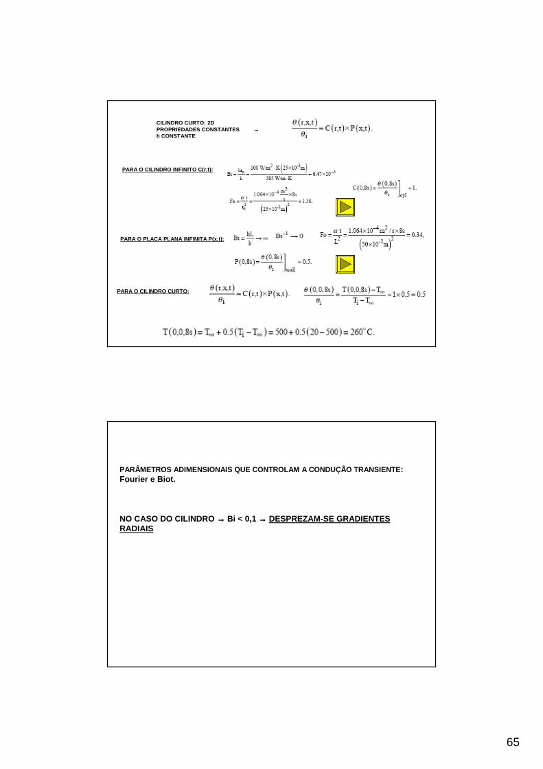
65

CILINDRO CURTO: 2D PROPRIEDADES CONSTANTES →→→→h CONSTANTE

PARA O CILINDRO INFINITO C(r,t):

PARA O PLACA PLANA INFINITA P(x,t):

PARA O CILINDRO CURTO:

PARÂMETROS ADIMENSIONAIS QUE CONTROLAM A CONDUÇÃO T RANSIENTE: Fourier e Biot.

NO CASO DO CILINDRO →→→→ Bi < 0,1 →→→→ DESPREZAM-SE GRADIENTES RADIAIS

66

5.90

Considerando que a carne fica cozida quando atinge uma temperatura de 80ºC,calcule o tempo necessário para assar uma peça de carne com 2,25 kg. Admitir que a peça de carne é um cilindro com diâmetro igual ao comprimento eque as suas propriedades são equivalentes às de água líquida. Considere que a carne se encontra inicialmente à temperatura de 6ºC e que atemperatura do forno é 175ºC e o coeficiente de convecção é de 15 W/m2K.

Propriedades da água :

CÁLCULO DAS DIMENSÕES DO CILINDRO:

CÁLCULO DA TEMPERATURA NO CENTRO DO CILINDRO:

67

SOLUÇÃO TENTATIVA-ERRO:

Introduction to Convection:Introduction to Convection:Flow and Thermal ConsiderationsFlow and Thermal Considerations

68

Boundary Layers: Physical Features• Velocity Boundary Layer

– A consequence of viscous effectsassociated with relative motionbetween a fluid and a surface.

– A region of the flow characterized byshear stresses and velocity gradients.

– A region between the surfaceand the free stream whosethickness increases in the flow direction.

δ( )

0.99u y

uδ

∞

→ =

– Why does increase in the flow direction?δ

– Manifested by asurface shearstress that provides a drag force, .

sτDF

0s y

u

yτ µ =

∂=∂

sD s s

A

F dAτ= ∫

– How does vary in the flowdirection? Why?

sτ

2

2

1∞

=u

C sf

ρ

τ

• Thermal Boundary Layer

– A consequence of heat transfer between the surface and fluid.

– A region of the flow characterizedby temperature gradients and heatfluxes.

– A region between the surface andthe free stream whosethicknessincreases in the flow direction.

tδ

– Why does increase in theflow direction?

tδ

– Manifested by asurface heatflux and a convection heattransfer coefficient h .

sq′′

( )0.99s

ts

T T y

T Tδ

∞

−→ =

−

0s f y

Tq k

y =∂′′ = −∂

0/f y

s

k T yh

T T

=

∞

− ∂ ∂≡

−– If is constant, how do and

h vary in the flow direction? ( )sT T∞−

sq′′

69

Distinction between LocalandAverageHeat Transfer Coefficients

• Local Heat Flux and Coefficient:

( )sq h T T∞′′ = −

• Average Heat Flux and Coefficient for a Uniform Surface Temperature:

( )s sq hA T T∞= −

s sAq q dA′′= ∫ ( )ss sAT T hdA∞= − ∫

1s sA

s

h hdAA

= ∫

• For aflat plate in parallel flow:

1 Loh hdx

L= ∫

Governing equationsGoverning equations

•• EquaEquaçção da continuidadeão da continuidade ( ) ( ) ( )0=

∂∂+

∂∂+

∂∂+

∂∂

z

w

y

v

x

u

t

ρρρρ

Equação de balanço da quantidade de movimento

( ) ( )i

j

ij

ij

iji gxx

p

x

uu

t

u ρτρρ

+∂∂

+∂∂−=

∂∂

+∂

∂

ijk

k

i

j

j

iij x

u

x

u

x

u δµµτ∂∂

−

∂∂

+∂∂

=3

2

Equação de conservação da energia

( ) ( ) qx

u

x

up

x

Tk

xeu

xe

t j

iij

j

j

jjj

j

′′′+∂∂

+∂∂

−

∂∂

∂∂=

∂∂+

∂∂

&τρρ• Energia interna

2

222222

2

3

2

2

3

2

∂∂

+∂∂

+∂∂

−

∂∂+

∂∂+

∂∂+

∂∂+

∂∂+

∂∂+

∂∂+

∂∂+

∂∂=

=

∂∂

−∂∂

∂∂

+∂∂

=∂∂

=Φ

z

w

y

v

x

u

y

w

z

v

x

w

z

u

x

v

y

u

z

w

y

v

x

u

x

u

x

u

x

u

x

u

x

u

k

k

j

i

i

j

j

i

j

iij

µ

µµ

µµτµDissipaçãoviscosa de energia

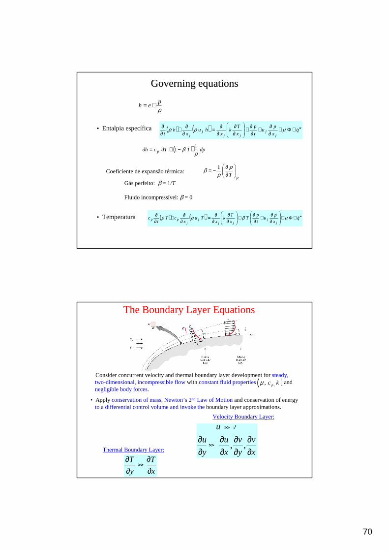
70

Governing equationsGoverning equations

( ) ( ) qx

pu

t

p

x

Tk

xhu

xh

t jj

jjj

j

′′′+Φ+∂∂+

∂∂+

∂∂

∂∂=

∂∂+

∂∂

&µρρ• Entalpia específica

( ) ( ) qx

pu

t

pT

x

Tk

xTu

xcT

tc

jj

jjj

jpp ′′′+Φ+

∂∂+

∂∂+

∂∂

∂∂=

∂∂+

∂∂

&µβρρ• Temperatura

ρp

eh +=

Coeficiente de expansão térmica:pT

∂∂−= ρ

ρβ 1

Gás perfeito: β = 1/T

Fluido incompressível: β = 0

( ) dpTdTcdh p ρβ 1

1−+=

The Boundary Layer Equations

• Consider concurrent velocity and thermal boundary layer development forsteady, two-dimensional, incompressible flowwith constant fluid properties and negligible body forces.

( ),, pc kµ

• Apply conservation of mass, Newton’s 2nd Law of Motionand conservation of energyto a differential control volume and invoke theboundary layer approximations.

Velocity Boundary Layer:

Thermal Boundary Layer:

T T

y x

∂ ∂∂ ∂

�>>

, ,

u v

u u v v

y x y x

∂ ∂ ∂ ∂∂ ∂ ∂ ∂

�

�

>>

>>

71

• Conservation of Mass:

0u v

x y

∂ ∂+ =∂ ∂

In the context of flow through a differential control volume, what is the physicalsignificance of the foregoing terms, if each is multiplied by the mass density of the fluid?

• Newton’s Second Law of Motion:

2

2

x-direction :

u u dp uu v

x u dx yρ µ∂ ∂ ∂ + = − + ∂ ∂ ∂

What is the physical significance of each term in the foregoing equation?

Why can we express the pressure gradient as dp/dx instead of / ?p x∂ ∂

y-direction :

0p

y

∂ =∂

What is the physical significance of each term in the foregoing equation?

What is the second term on the right-hand side called and under what conditionsmay it be neglected?

• Conservation of Energy:

22

2p

T T T uc u v k

x y y yρ µ ∂ ∂ ∂ ∂+ = + ∂ ∂ ∂ ∂

72

Boundary Layer Similarity• As applied to the boundary layers, the principle of similitudeis based on

determiningsimilarity parametersthat facilitate application of results obtainedfor a surface experiencing one set of conditions to geometrically similar surfacesexperiencing different conditions. (Recall how introduction of the similarityparameters Bi and Fo permitted generalization of results for transient, one-dimensional condition).

• Dependent boundary layer variablesof interest are:

and or s q hτ ′′

• For a prescribed geometry, the correspondingindependent variablesare:

Geometrical:Size (L), Location (x,y)Hydrodynamic:Velocity (V)Fluid Properties:

Hydrodynamic: ,

Thermal : ,pc k

ρ µ

( )( )

Hence,

, , , , ,

, , , ,s

u f x y L V

f x L V

ρ µτ ρ µ

=

=

( )( )

and

, , , , , , ,

, , , , , ,

p

p

T f x y L V c k

h f x L V c k

ρ µ

ρ µ

=

=

• Key similarity parameters may be inferred by non-dimensionalizing the momentumand energy equations.

• Recast the boundary layer equations by introducing dimensionless forms of theindependent and dependent variables.

* *

* *

* s

s

x yx y

L Lu v

u vV V

T TT

T T∞

≡ ≡

≡ ≡

−≡

−

• Neglecting viscous dissipation, the following normalizedforms of the x-momentum and energy equations are obtained: * * * 2 *

* ** * * *2

* * 2 ** *

* * *2

1

Re

1

Re Pr

L

L

u u dp uu v

x y dx y

T T Tu v

x y y

∂ ∂ ∂+ = − +∂ ∂ ∂

∂ ∂ ∂+ =∂ ∂ ∂

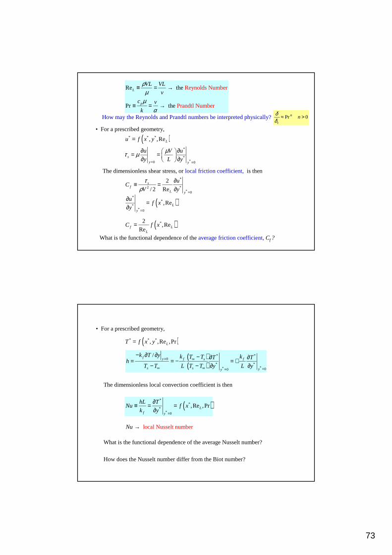
73

Reynolds NumbeRe the

Pr

r

Prandtl Number the

L

p

VL VL

v

c v

k

ρµ

µα

≡ = →

≡ = →

• For a prescribed geometry,

( )* * *, ,ReLu f x y=

*

*

*0 0

s

y y

u V u

y L y

µτ µ= =

∂ ∂ = = ∂ ∂

The dimensionless shear stress, orlocal friction coefficient, is then

*

*

2 *0

2

/ 2 Res

fL y

uC

V y

τρ

=

∂≡ =

∂

( )*

**

*0

,ReL

y

uf x

y=

∂=

∂

( )*2,Re

Ref LL

C f x=

What is the functional dependence of theaverage friction coefficient,Cf ?

How may the Reynolds and Prandtl numbers be interpreted physically? 0Pr >≈ nn

tδδ

• For a prescribed geometry,

( )* * *, ,Re ,PrLT f x y=

( )( ) **

* *0

* *

00

/f y f fs

s s yy

k T y k kT T T Th

T T L T T y L y= ∞

∞ ∞ ==

− ∂ ∂ − ∂ ∂= = − = +− − ∂ ∂

The dimensionless local convection coefficient is then

( )*

**

*

0

,Re ,PrLf y

hL TNu f x

k y=

∂≡ = =

∂

local Nusselt nu mberNu →

What is the functional dependence of the average Nusselt number?

How does the Nusselt number differ from the Biot number?

74

Boundary Layer Transition

• How would you characterize conditions in the laminar regionof boundary layerdevelopment?In the turbulent region?

• What conditions are associated withtransitionfrom laminar to turbulent flow?

• Why is the Reynolds number an appropriate parameter for quantifying transitionfrom laminar to turbulent flow?

• Transition criterionfor a flat plate in parallel flow:

, critical Rey nolds numberRe cx c

u xρµ∞≡ →

location at which transition to turbulence beginscx →5 6

,~ ~

10 Re 3 x 10x c< <

Why does it increase significantly with transition to turbulence, despite the increase in the boundary layerthickness?

What may be said about transition if ReL < Rex,c? If ReL > Rex,c?

• Effect of transition on boundary layer thickness and local convection coefficient:

Why does transition provide a significant increase in the boundary layer thickness?

Why does the convection coefficient decay in the laminar region?

Why does the convection coefficient decay in the turbulent region?

75

The Reynolds Analogy• Equivalence of dimensionless momentum and energy equations for

negligible pressure gradient (dp*/dx*~0) and Pr~1:

Advection terms Diffusion

* * 2 ** *

* * *2

1

Re

T T Tu v

x y y

∂ ∂ ∂+ =∂ ∂ ∂

* * 2 ** *

* * *2

1

Re

u u uu v

x y y

∂ ∂ ∂+ =∂ ∂ ∂

• Hence, for equivalent boundary conditions, the solutions are of the same form:

* *

* *

* *

* *0 0

Re

2

y y

f

u T

u T

y y

C Nu

= =

=

∂ ∂=∂ ∂

=

With Pr = 1, the Reynolds analogy, which relates important parameters of the velocityand thermal boundary layers, is

2fC

St=

or, with the defined asStanton number ,

p

h NuSt

Vc Re Prρ≡ =

• Modified Reynolds (Chilton-Colburn) Analogy:

– An empirical result that extends applicability of the Reynolds analogy:

23Pr 0.6 Pr 60

2f

H

CSt j= ≡ < <

Colburn j factor for heat transfer

– Applicable to laminar flow if dp*/dx* ~ 0.

– Generally applicable to turbulent flow without restriction on dp*/dx*.

76

Problem 6.28: Determination of heat transfer rate for prescribed turbine blade operating conditions from wind tunnel data obtained for a geometrically similar but smaller blade. The blade surface area may be assumed to be directly proportional to its characteristic length . ( )sA L∝

SCHEMATIC:

ASSUMPTIONS: (1) Steady-state conditions, (2) Constant properties, (3) Surface area A is directly proportional to characteristic length L, (4) Negligible radiation, (5) Blade shapes are geometrically similar.

ANALYSIS: For a prescribed geometry,

( )LhL

Nu f Re ,Pr .k

= =

The Reynolds numbers for the blades are

( ) ( )2 2L,1 1 1 1 1 L,2 2 2 2 2Re V L / 15m / s Re V L / 15m / s .ν ν ν ν= = = =

Hence, with constant properties ( )1 2v v= , L,1 L,2Re Re .= Also, 1 2Pr Pr=

Therefore, 2 1Nu Nu=

( ) ( )2 2 2 1 1 1h L / k h L / k=

( )1 1 1

2 12 2 1 s,1

L L qh h

L L A T T∞= =

−

The heat rate for the second blade is then

( ) ( )( )

s,21 22 2 2 s,2 1

2 1 s,1

T TL Aq h A T T q

L A T T

∞∞

∞

−= − =

−

( )( ) ( )s,2

2 1s,1

T T 400 35q q 1500 W

T T 300 35∞

∞

− −= =

− −2q 2066 W.=

COMMENTS: (i) The variation in ν from Case 1 to Case 2 would cause ReL,2 to differ from

ReL,1. However, for air and the prescribed temperatures, this non-constant property effect is small. (ii) If the Reynolds numbers were not equal ( ),1 2Re Re ,L L≠ knowledge of the specific form of

( ),Re PrLf would be needed to determine h2.

77

Problem 6.35: Use of a local Nusselt number correlation to estimate thesurface temperature of a chip on a circuit board.

KNOWN: Expression for the local heat transfer coefficient of air at prescribed velocity and temperature flowing over electronic elements on a circuit board and heat dissipation rate for a 4 × 4 mm chip located 120mm from the leading edge.

FIND: Surface temperature of the chip surface, Ts.

SCHEMATIC:

ASSUMPTIONS: (1) Steady-state conditions, (2) Power dissipated within chip is lost by convection across the upper surface only, (3) Chip surface is isothermal, (4) The average heat transfer coefficient for the chip surface is equivalent to the local value at x = L.

PROPERTIES: Table A-4, Air (Evaluate properties at the average temperature of air in the boundary

layer. Assuming Ts = 45°C, Tave = (45 + 25)/2 = 35°C = 308K. Also, p = 1atm): ν = 16.69 ×

10-6

m2/s, k = 26.9 × 10

-3 W/m⋅K, Pr = 0.703.

ANALYSIS: From an energy balance on the chip,

conv gq E 30mW.= =&

Newton’s law of cooling for the upper chip surface can be written as

s conv chipT T q / h A∞= + (2)

where 2chipA .= l

Assuming that the average heat transfer coefficient ( )h over the chip surface is equivalent to the local

coefficient evaluated at x = L, that is, ( )chip xh h L≈ , the local coefficient can be evaluated by

applying the prescribed correlation at x = L.

0.85

1/ 3xx

h x VxNu 0.04 Pr

k ν = =

0.85

1/ 3L

k VLh 0.04 Pr

L ν =

78

( )0.85

1/ 3 2L -6 2

0.0269 W/m K 10 m/s 0.120 mh 0.04 0.703 107 W/m K.

0.120 m 16.69 10 m / s

⋅ × = = ⋅ ×

From Eq. (2), the surface temperature of the chip is

( )2-3 2sT 25 C 30 10 W/107 W/m K 0.004m 42.5 C.= + × ⋅ × =o o

COMMENTS: (1) The estimated value of Tave used to evaluate the air properties is reasonable.

(2) How else could chiph have been evaluated? Is the assumption of Lh h= reasonable?

External Flow:External Flow:The Flat Plate in Parallel FlowThe Flat Plate in Parallel Flow

79

Physical Features

• As with all external flows, the boundary layers develop freely without constraint.

• Boundary layer conditions may be entirely laminar, laminar and turbulent,or entirely turbulent.

• To determine the conditions, compute

and compare with thecritical Reynolds numberfor transition to turbulence,

ReL

u L u Lρµ ν

∞ ∞= =

,Re .x c

, laminar flow tRe Re hroughout L x c< →

, ,transition to turbulent flowRe Re at / Re R e /L x c c x c Lx L> → ≡

sT sq′′• Surface thermal conditionsare commonly idealized as being ofuniform

temperature or uniform heat flux .Is it possible for a surface to be concurrently characterized by uniform temperature and uniform heat flux?

,Rex c• Value of depends on free stream turbulence and surface roughness. Nominally,

5

, 5 10Re .x c ×≈

• If boundary layer istrippedat the leading edge

and theflow is turbulent throughout.

,Re 0x c =

• Thermal boundary layer development may be delayed by anunheatedstarting length.

Equivalent surface and free stream temperatures for and uniform (or ) for .

x ξ< sT

sq′′ .x ξ>

80

Similarity Solution for Laminar, Constant-Property Flow over an Isothermal Plate

• Based on premise that the dimensionless x-velocity component, ,and temperature, , can be represented exclusively interms of adimensionless similarity parameter

/u u∞( ) ( )* /s sT T T T T∞ ≡ − −

( )1/ 2/y u xη ν∞≡

• Similarity permits transformation of the partial differential equations associatedwith the transfer of x-momentum and thermal energy to ordinary differentialequations of the form

3 2

3 22 0d f d f

fd dη η

+ =

( )where / / , ∞ ≡u u df dη and

2 * *

2

Pr0

2+ =d T dT

fd dη η

Similarity Solution for Laminar, Constant-Property Flow over an Isothermal Plate

81

• Subject to prescribed boundary conditions, numerical solutions to the momentumand energy equations yield the following results for importantlocal boundary layerparameters:

( )1/ 2

- with / 0.99 at 5

5.0 5

R

. ,

e/

0

x

x

u

u

vx

u η

δ∞

∞

= =

= =

2

20 0

- with /s

y

u d fu u vx

y d η

τ µ µη∞ ∞

= =

∂= =

∂

2 2

0and / 0.332,d f d

ηη

==

, 1/ 2, 2 0.664Re

/ 2 x

s xf xC

u

τρ

−

∞

≡ =

( ) ( )1/ 2* *

0 0- with / / / /x s s y

h q T T k T y k u vx dT dη

η∞ ∞= =′′= − = ∂ ∂ =

* 1/ 3

0and / 0.332 Pr for Pr 0.6,dT d

ηη

== >

1/ 3

r

and

Pt

δδ

=

1/ 2 1/ 30.332 Re Prxx x

h xNu

k= =

• How would you characterize relative laminar velocity and thermal boundary layergrowth for a gas? An oil? A liquid metal?

• How do the local shear stress and convection coefficient vary with distance fromthe leading edge?

• Average Boundary Layer Parameters:

, 0

1 xs x sdx

xτ τ≡ ∫

1/ 2, 1.328 Re

xf xC −=

0

1 xx xh

xh dx= ∫

1/ 2 1/ 30.664 Re Prx xNu =• The effect of variable properties may be considered by evaluating all properties

at thefilm temperature.

2s

f

T TT ∞+=

82

( )4 / 5 1/ 30.037 Re 871 PrL LNu = −

Turbulent Flow• Local Parameters:

1/ 5,

4 / 5 1/ 3

0.0592 Re

0.0296 Re Pr

f x x

x x

C

Nu

−=

=Empirical

Correlations

How do variations of the local shear stress and convection coefficient withdistance from the leading edge for turbulent flow differ from those for laminar flow?

• Average Parameters:

( )10

1c

c

x LL am turbxh h dx h dx

L= +∫ ∫

Substituting expressions for the local coefficients andassuming 5

x,cRe 5 10,= ×

, 1/ 5

0.074 1742

Re Ref LL L

C = −

( ), ,

1/ 5,

4 / 5 1/ 3

For Re 0 or Re Re ,

0.074 Re

0.037 Re Pr

x c c L x c

f L L

L L

L x

C

Nu

−

=

=

=

� �»»

Special Cases: Unheated Starting Length (USL)and/or Uniform Heat Flux

For both uniform surface temperature (UST) and uniform surface heat flux (USF),the effect of the USL on thelocalNusselt number may be represented as follows:

( )0

1/ 30

1 /

Re Pr

x

x ba

mx x

NuNu

x

Nu C

ξ

ξ

ξ

=

=

= −

=4/54/54/54/51/21/21/21/2mm

0.03080.03080.02960.02960.4530.4530.3320.332CC

1/91/91/91/91/31/31/31/3bb

9/109/109/109/103/43/43/43/4aa

USFUSFUSTUSTUSFUSFUSTUST

TurbulentTurbulentLaminarLaminar

Sketch the variation of hx versus for two conditions: What effect does an USL have on the local convection coefficient?

( )x ξ− 0 and 0.ξ ξ> =

83

• UST:

( )s x sq h T T∞′′ = −

( ) ( )( ) ( ) ( )2 / 2 12 1 / 2 2

0

lamina

1 /

1 for throughout

= 4 for througho

r flow

turbulent

w uflo t

p pp pL L

LNu Nu L

L

p

p

ξξ

ξ

++ +

= = − −

=

1

laminar/turbulent flow numerical integration f

1

or

c

c

L

x LL am turbx

h

h h dx h dxL ξ

→

= +∫ ∫

• USF:s

sx

qT T

h∞′′

= +s sq q A′′=

• Treatment of Non-Constant Property Effects:

Evaluate properties at thefilm temperature.

2s

f

T TT ∞+=

( )∞= −L s sq h A T T

Problem 7.21: Preferred orientation (corresponding to lower heat loss) and the corresponding heat rate for a surface with adjoining smooth and roughened sections.

SCHEMATIC:

ASSUMPTIONS: (1) Surface B is sufficiently rough to trip the boundary layer when in the upstream position

(Configuration 2); (2) 55 10,Re for flow over A in Configuration 1.×≈x c

84

PROPERTIES: Table A-4, Air (Tf = 333K, 1 atm): ν = 19.2 × 10-6

m2/s, k = 28.7 × 10

-3

W/m⋅K, Pr = 0.7.

ANALYSIS: Since Configuration (2) results in a turbulent boundary layer over the entire surface, the lowest heat transfer is associated with Configuration (1).

Find

6L -6 2

u L 20 m/s 1mRe 1.04 10 .

19.2 10 m / sν∞ ×= = = ×

×

Hence in Configuration (1), transition will occur just before the rough surface (xc = 0.48m).

( )L,1

4 / 56 1/3Nu 0.037 1.04 10 871 0.7 1366

= × − =

For Configuration (1): L,1L,1h L

Nu 6k

.136= =

Hence

( )3 2L,1h 1366 28.7 10 W/m K /1m 39.2 W/m K−= × ⋅ = ⋅

1568 W= < ( ) ( )( )21 L,1 sq h A T T 39.2 W/m K 0.5m 1m 100 20 K∞= − = ⋅ × −

Comment: Note that ( ) ( )L,2 L,1

4 / 5 1/ 36Nu 0.037 1.04 10 0.7 2139 Nu .= × = >

External Flow:External Flow:Flow over Bluff ObjectsFlow over Bluff Objects

(Cylinders, Sphere)(Cylinders, Sphere)

85

The Cylinder in Cross Flow• Conditions depend on special features of boundary layer development, including

onset at astagnation pointand separation, as well astransition to turbulence.

– Stagnation point:Location ofzero velocity andmaximum pressure.( )0u∞ =

– Followed by boundary layer development under afavorable pressure gradientand hence acceleration of the free stream flow .( )/ 0dp dx< ( )/ 0du dx∞ >

– As the rear of the cylinder is approached, the pressure must begin to increase. Hence, there is a minimum in the pressure distribution, p(x), after which boundarylayer development occurs under the influence of anadverse pressure gradient( )/ 0, / 0 .dp dx du dx∞> <

– Separationoccurs when the velocity gradient reduces to zero.0/ ydu dy =

and is accompanied byflow reversaland a downstreamwake.

– Location of separation depends onboundary layer transition.

ReD

VD VDρµ ν

≡ =

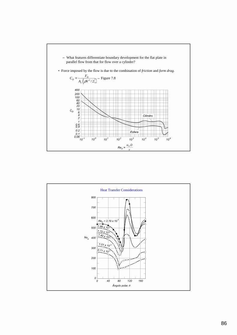
86

– What features differentiate boundary development for the flat plate inparallel flow from that for flow over a cylinder?

• Force imposed by the flow is due to the combination of friction and form drag.

The dimensionless form of the drag force is

( )2Figure 7.8

/ 2D

D

f

FC

A Vρ= →

• Heat Transfer Considerations

87

• Heat Transfer Considerations

θ 5Re 2 10D < x

– How does the local Nusselt vary with 5 for Re 2 10 ?θ >D

x

– TheLocal Nusselt Number:

– How does the local Nusselt number vary with for ?What conditions are associated with maxima and minima in the variation?

What conditions are associated with maxima and minima in the variation?

– TheAverage Nusselt Number( )/ :DNu hD k≡

– Churchill and Bernstein Correlation:

( )

4 / 55 / 81/ 2 1/ 3

1/ 42 / 3

0.62Re Pr Re0.3 1

282,0001 0.4 / Pr

D DDNu

= + + +

– Cylinders of Noncircular Cross Section:

1/ 3Re PrmD DNu C=

, Table 7.3C m→

0.8050.0274×104 – 4×105

0.6180.1934×103 – 4×104

0.4660.68340 – 4×103

0.3850.9114 – 40

0.3300.9890.4 – 4

mCReD

Flow Across Tube Banks

• A common geometry fortwo-fluid heat exchangers.

maxSTV V

S DT=

−

• Aligned and Staggered Arrays:

Aligned:

Staggered: ( ) ( )if 2maxSTV V S D S DD TS DT

= − ≥ −−

( ) ( ) ( )if 2max 2

STV V S D S DD TS DD= − ≤ −

−or,

88

• Flow Conditions:

How do convection coefficients vary from row-to-row in an array?

How do flow conditions differ between the two configurations?

Why should an aligned array not be use for ST/SL < 0.7?

• Average Nusselt Number for an Isothermal Array:

( )1/ 40.362 ,maxRe Pr Pr/ Prm

D D sNu C C =

2

, Table 7.7

Table 7.8

C m

C

→→

All properties are evaluated at except for Prs.( ) / 2i oT T+

0.840.0222×105 - 2×106

0.600.40103 - 2×105 (ST / SL > 2)

0.600.35 (ST / SL)1/5103 - 2×105 (ST / SL < 2)

Aproximado por um tubo isolado

102 – 103

0.400.9010 - 102

Tubos desfasados

0.840.0212×105 - 2×106

0.630.27103 - 2×105 (ST /SL <

0.7)*

Aproximado por um tubo isolado

102 – 103

0.400.8010 - 102

Tubos alinhados

mCReD,maxGeometria

0.990.980.970.950.920.890.840.760.64Desfasados

0.990.980.970.950.920.900.860.800.70Alinhados

161310754321NL

89

• Fluid Outlet Temperature (To) :

s o

s i T T p

T T DNhexp

T T VN S c

− π= − − ρ

T LN N N= x

What may be said about To as ?N → ∞

• Total Heat Rate:

s mq hA T= ∆ l

( )sA N DLπ=( ) ( )s i s o

m

s i

s o

T T T TT

T Tn

T T

− − −∆ =

− −

l

l

• Pressure Drop:2

max

2L

Vp N f

ρχ

∆ =

, Figures 7.13 and 7.14fχ →

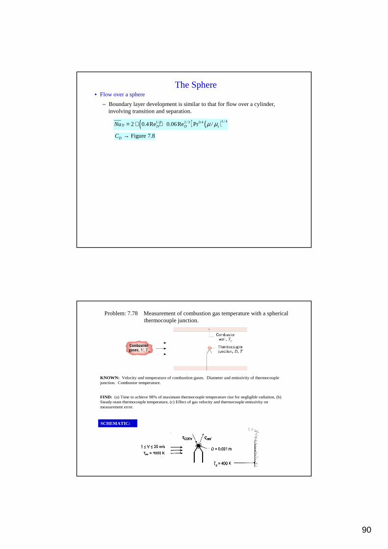
90

The Sphere• Flow over a sphere

– Boundary layer development is similar to that for flow over a cylinder, involving transition and separation.

( ) ( )1/ 41/ 2 2 / 3 0.42 0.4Re 0.06Re Pr /D D D sNu µ µ= + +

Figure 7.8DC →

Problem: 7.78 Measurement of combustion gas temperature with a sphericalthermocouple junction.

KNOWN: Velocity and temperature of combustion gases. Diameter and emissivity of thermocouple junction. Combustor temperature.

FIND: (a) Time to achieve 98% of maximum thermocouple temperature rise for negligible radiation, (b) Steady-state thermocouple temperature, (c) Effect of gas velocity and thermocouple emissivity on measurement error.

SCHEMATIC:

91

ASSUMPTIONS: (1) Validity of lumped capacitance analysis, (2) Constant properties, (3) Negligible conduction through lead wires, (4) Radiation exchange between small surface and a large enclosure (parts b and c).

PROPERTIES: Thermocouple: 0.1 ≤ ε ≤ 1.0, k = 100 W/m⋅K, c = 385 J/kg⋅K, ρ = 8920 kg/m3; Gases: k = 0.05 W/m⋅K, ν = 50 × 10-6 m2/s, Pr = 0.69.

ANALYSIS: (a) If the lumped capacitance analysis may be used, it follows from Equation 5.5 that

( )i

s

T TVc D ct ln ln 50

T ThA 6h

ρ ρ∞∞

−= =

−.

Neglecting the viscosity ratio correlation for variable property effects, use of V = 5 m/s with the Whitaker correlation yields

( ) ( )1/ 2 2 / 3 0.4D D DNu hD k 2 0.4 Re 0.06 Re Pr= = + +

( ) ( )( )( )1/ 2 2 / 3 0.4 20.05W m Kh 2 0.4 100 0.06 100 0.69 328W m K

0.001m

⋅ = + + = ⋅

Since Bi = ( )oh r 3 k = 5.5 × 10-4, the lumped capacitance method may be used.

( )( )

3

2

0.001m 8920kg m 385J kg Kt ln 50 6.83s

6 328W m K

⋅= =

× ⋅

(b) Performing an energy balance on the junction, qconv = qrad.

Hence, evaluating radiation exchange from Equation 1.7 and with ε = 0.5,

( ) ( )4 4s s chA T T A T Tε σ∞ − = −

( ) ( )8 2 4

44 42

0.5 5.67 10 W m K1000 T K T 400 K

328W m K

−× × ⋅ − = − ⋅

T = 936 K

Parametric calculations to determine the effects of V and ε yield the following results:

0 5 10 15 20 25

Velocity, V(m/s)

900

950

1000

Tem

pera

ture

, T(K

)

Emissivity, epsilon = 0.5

0.1 0.2 0.3 0.4 0.5 0.6 0.7 0.8 0.9 1

Emissivity

890

910

930

950

970

990

Tem

pera

ture

, T

(K)

Velocity, V = 5 m/s

92

Since the temperature recorded by the thermocouple junction increases with increasing V and decreasing ε, the measurement error, T∞ - T, decreases with increasing V and decreasing ε. The error is due to net

radiative transfer from the junction (which depresses T) and hence should decrease with decreasing ε.

For a prescribed heat loss, the temperature difference (T∞ - T) decreases with decreasing convection

resistance, and hence with increasing h(V).

COMMENTS: To infer the actual gas temperature (1000 K) from the measured result (936 K), correction would have to be made for radiation exchange with the cold surroundings.

What measures may be taken to reduce the error associated with radiation effects?

Internal Flow:Internal Flow:General ConsiderationsGeneral Considerations

93

Entrance Conditions• Must distinguish betweenentrance andfully developed regions.

• Hydrodynamic Effects: Assume laminar flow with uniform velocity profile atinlet of a circular tube.

– Velocity boundary layerdevelops on surface of tube and thickens with increasing x.

– Inviscid region of uniform velocity shrinks as boundary layer grows.

� Does the centerline velocity change with increasingx? If so, how does it change?

– Subsequent to boundary layer merger at the centerline, the velocity profilebecomesparabolicand invariant with x. The flow is then said to behydrodynamically fully developed.

� How would the fully developed velocity profile differ for turbulent flow?

• Thermal Effects:Assume laminar flow with uniform temperature, , atinlet of circular tube withuniform surface temperature, , orheat flux, .

( ),0 iT r T=s iT T≠ sq′′

– Thermal boundary layerdevelops on surface of tube and thickens with increasing x.

– Isothermal core shrinks as boundary layer grows.

– Subsequent to boundary layer merger,dimensionlessforms of the temperatureprofile become independent of x.( )for and s sT q′′

� Is the temperature profile invariant with x in the fully developed region?

94

� For uniform surface temperature, what may be said about the changein the temperature profile with increasing x?

� For uniform surface heat flux, what may be said about the change in thetemperature profile with increasing x?

� How do temperature profiles differ for laminar and turbulent flow?

The Mean Velocity and Temperature• Absence of well-defined free stream conditions, as in external flow, and hence a

reference velocity or temperature , dictates the use of a cross-sectional mean velocity and temperature for internal flow.

( )u∞ ( )T∞

( )mu ( )mT

( )or,

,cA cm u r x dAρ= ∫

�

( )Hence,

,cA c

mc

u r x dAu

A

ρρ

∫=

( )2

2,

or

m o

o

u u r x r drr

= ∫

• Linkage ofmean velocityto mass flow rate:

m cm u Aρ=�

For incompressible flowin a circular tubeof radius , or

95

• Linkage ofmean temperatureto thermal energy transportassociated with flow through a cross section:

ct A c mE uc T dA mc Tυ υρ= ∫ ≡

� �

Hence,

cA cm

uc T dAT

mc

υ

υ

ρ∫=

�

• For incompressible, constant-property flow in a circular tube,

( ) ( )02

2, ,

or

m

m o

T u x r T x r r dru r

= ∫

• Newton’s Law of Cooling for the Local Heat Flux:

( )s s mq h T T′′ = −

What is the essential difference between use of for internal flow andfor external flow?

mT T∞

Hydrodynamic and Thermal Entry Lengths

• Entry lengths depend on whether the flow is laminar or turbulent, which, in turn,depend on Reynolds number.

Re m hD

u Dρµ

≡

The hydraulic diameteris defined as

4 ch

AD

P≡

in which case,

4Re m h

D

u D m

P

ρµ µ

≡ =�

For a circular tube,

4Re m

D

u D m

D

ρµ π µ

= =�

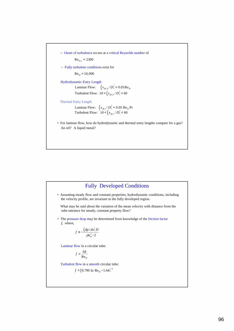
96

– Onset of turbulenceoccurs at acritical Reynolds numberof

,Re 2300D c ≈

– Fully turbulent conditionsexist for

Re 10,000D ≈

• Hydrodynamic Entry Length

( ),Laminar Flow: / 0.05Refd h Dx D ≈

( ),Turbulent Flow: 10 / 60fd hx D< <

• For laminar flow, how do hydrodynamic and thermal entry lengths compare for a gas?An oil? A liquid metal?

( ),Laminar Flow: / 0.05 Re Prfd t Dx D ≈• Thermal Entry Length

( ),Turbulent Flow: 10 / 60fd tx D< <

Fully Developed Conditions

• Assuming steady flow and constant properties, hydrodynamic conditions, includingthe velocity profile, are invariant in the fully developed region.

What may be said about the variation of the mean velocity with distance from thetube entrance for steady, constant property flow?

• The pressure dropmay be determined from knowledge of thefriction factorf, where,

( )2

/

/ 2m

dp dx Df

uρ≡ −

Laminar flowin a circular tube:

64

ReD

f =

Turbulent flowin asmoothcircular tube:

( ) 20.790 1n Re 1.64Df

−= −

97

Turbulent flowin a roughened circular tube:

Pressure dropfor fully developed flow from x1 to x2:

( )2

1 2 2 12mu

p p p f x xD

ρ∆ = − = −

andpower requirement

pmP p

ρ∆

= ∆ ∀ =�

�

• Requirement for fully developed thermal conditions:

( ) ( )( ) ( )

,

,0s

s m fd t

T x T r x

x T x T x

−∂ = ∂ −

• Effect on the local convection coefficient:

( )/

o

o

r rs

s m s mr r

T rT Tf x

r T T T T=

=

−∂ ∂ −∂ = ≠ ∂ − −

Hence, assuming constant properties,

( )/s

s m

q k hf x

T T k

′′= ≠

−

( )h f x≠

Variation of h in entrance and fully developed regions:

98

Determination of the Mean Temperature

• Determination of is an essential feature of an internal flow analysis.( )mT x

Determination begins with an energy balance for a differential control volume.

( )conv m p mdq md c T p mc dTυ υ= + ≈� �

Why is the second equality in the foregoing expression considered to be approximate?

Integrating from the tube inlet to outlet,

( ), , (1)conv p m o m iq mc T T= −�

A differential equation from which may be determined is obtained bysubstituting for

( )mT x( ) ( ) .

conv s s mdq q Pdx h T T Pdx′′= = −

( ) ( )2m ss m

p p

dT q P Ph T T

dx mc mc

′′= = −

� �

• Special Case: Uniform Surface Heat Flux

( )m s

p

dT q Pf x

dx mc

′′= ≠

�

( ) ,s

m m i

p

q PT x T x

mc

′′= +

�

Why does the surface temperature vary with x as shown in the figure?

In principle, what value does Ts assume atx=0?

Total heat rate:

conv sq q PL′′=

99

• Special Case: Uniform Surface Temperature

( )From Eq. (2), with s m

m

p

T T T

d Td T Ph T

dx dx mc

∆ ≡ −∆

= − = ∆�

Integrating from x=0 to any downstream location,

( ),

exps mx

s m ip

T T x Pxh

T T mc

− = − −

�

1x x

xoh h dx

x= ∫

Overall Conditions:

,

,

exp exps m oo s

i s m ip p

T TT h APLh

T T T mc mc

−∆ = = − = − ∆ −

� �

conv s mq h A T= ∆ l

( ) ( )31n /

o im

o i

T TT

T T

∆ − ∆∆ =∆ ∆l

• Special Case:Uniform ExternalFluid Temperature

,

,

1exp expm oo s

i m ip p tot

T TT U A

T T T mc mc R

∞

∞

−∆ = = − = − ∆ −

��

ms m

tot

Tq UA T

R

∆= ∆ = l

l

Eq. (3) with replaced by .m sT T T∞∆ →l

Note: Replacement of by Ts,o if outer surface temperature is uniform.T∞

100

Problem 8.17: Estimate temperature of water emerging from a thin-walledtube heated by walls and air of a furnace. Inner and outerconvection coefficients are known.

KNOWN: Water at prescribed temperature and flow rate enters a 0.25 m diameter, black thin-walled tube of 8-m length, which passes through a large furnace whose walls and air are at a temperature of Tfur = T∞ = 700 K. The convection coefficients for the internal water flow and external furnace air are 300 W/m2⋅K and 50 W/m2⋅K, respectively.

FIND: The outlet temperature of the water, Tm,o.

SCHEMATIC :

ASSUMPTIONS: (1) Steady-state conditions; (2) Tube is small object with large, isothermal surroundings; (3) Furnace air and walls are at the same temperature; and (3) Tube is thin-walled with black surface.

PROPERTIES: Table A-6, Water: cp ≈ 4180 J/kg⋅K.

ANALYSIS: The linearized radiation coefficient may be estimated from Eq. 1.9 with ε = 1,

( )( )2 2rad t fur t furh T T T Tσ≈ + +

where tT represents the average tube wall surface temperature, which can be estimated from an energy balance

on the tube.

As represented by the thermal circuit, the energy balance may be expressed as m t t fur

cv,i cv,o rad

T T T T

R 1/ R 1/ R

− −=

+

The thermal resistances, with As = PL = πDL, are

cv,i i s cv,o o s rad radR 1/ h A R 1/ h A R 1/ h= = =

101

and the mean temperature of the water is approximated as

( )m m,i m,oT T T / 2= +

The outlet temperature can be calculated from Eq. 8.46b, with Tfur = T∞,

T T 1expT T

m c R

m,o

m,ip tot

− = −

−

∞∞ �

where

tot cv,icv,o rad

1R R

1/ R 1/ R= +

+

with 5 4 4

cv,i cv,o radR 6.631 10 K / W R 3.978 10 K / W R 4.724 10 K / W− − −= × = × = ×

it follows that

m tT 331 K T 418 K= = m,oT 362 K=

Internal Flow:Internal Flow:Heat Transfer CorrelationsHeat Transfer Correlations

102

Fully Developed Flow• Laminar Flow in a Circular Tube:

Thelocal Nusselt numberis aconstantthroughout the fully developedregion, but its value depends on the surface thermal condition.

( )sq′′– Uniform Surface Heat Flux :

4.36DhDNuk

= =

( )sT– Uniform Surface Temperature :

3.66DhDNuk

= =

( )( )( ) ( )1/ 2 2 / 3

/8 Re 1000 Pr

1 12.7 /8 Pr 1D

D

fNu

f

−=

+ −

– The effects ofwall roughnessand transitional flowconditions may be considered by using theGnielinski correlation:

( )Re 3000D >

( )Re 10,000D >• Turbulent Flowin aCircular Tube:

– For asmooth surfaceand fully turbulent conditions , theDittus – Boelter equationmay be used as a first approximation:

4 / 50.023Re PrnD DNu = ( )( )

0.30.4

s m

s m

n T Tn T T

= <= >

Smooth surface:

( ) 20.790 1n Re 1.64Df

−= −

Surface of roughness :0e>

Figure 8.3f →

• Noncircular Tubes:– Use ofhydraulic diameteras characteristic length:

4 ch

AD

P≡

– Since the local convection coefficient varies around the periphery of a tube,approaching zero at its corners, correlations for the fully developed regionare associated with convection coefficients averaged over the peripheryof the tube.

– Laminar Flow:

The local Nusselt number is a constant whose value(Table 8.1)depends onthe surface thermal condition and the duct aspect ratio.( ) s sT or q′′

– Turbulent Flow:

As a first approximation, the Dittus-Boelter or Gnielinski correlation may be used with the hydraulic diameter, irrespective of the surface thermal condition.

103

Effect of the Entry Region• The manner in which the Nusselt decays from inlet to fully developed conditions

for laminar flow depends on the nature of thermal and velocity boundary layerdevelopment in the entry region, as well as the surface thermal condition.

Laminar flow in acircular tube.

– Combined Entry Length:

Thermal and velocity boundary layers develop concurrently from uniformprofiles at the inlet.

– Thermal Entry Length:

Velocity profile is fully developed at the inlet, and boundary layer development in the entry region is restricted to thermal effects. Such a condition may alsobe assumed to be a good approximation for a uniform inlet velocity profile if Pr 1.>> Why?

• Average Nusselt Number for Laminar Flow in a Circular Tube with UniformSurface Temperature:– Combined Entry Length:

( ) ( )1/ 3 0.14Re Pr/ / / 2 :D sL D µ µ >

0.141/ 3Re Pr

1.86/D

D

s

NuL D

µµ =

( ) ( )1/ 3 0.14Re Pr/ / / 2 :D sL D µ µ <

3.66DNu =– Thermal Entry Length:

( )( ) 2 / 3

0.0668 / Re Pr3.66

1 0.04 / Re PrD

D

D

D LNu

D L= +

+

104

• Average Nusselt Number for Turbulent Flow in a Circular Tube :

– Effects of entry and surface thermal conditions are less pronounced forturbulent flow and can be neglected.

– For long tubes :( )/ 60L D >

,D D fdNu Nu≈

– For short tubes : ( )/ 60L D <

( ),

1/

Dm

D fd

Nu CNu L D

≈ +

12/3

Cm

≈≈

• Noncircular Tubes:

– Laminar Flow:

depends strongly on aspect ratio, as well as entry region and surfacethermal conditions.

hDNu

• When determining for any tube geometry or flow condition, all properties are to be evaluated at

DNu

( ), , / 2m m i m oT T T≡ +

Why do solutions to internal flow problems often require iteration?

– Turbulent Flow:

As a first approximation, correlations for a circular tube may be usedwith D replaced by .hD

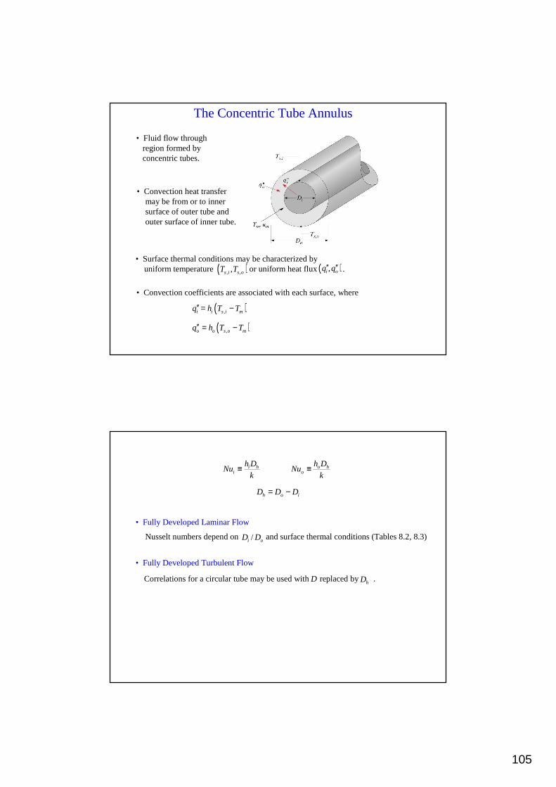
105

The Concentric Tube Annulus

• Fluid flow throughregion formed by concentric tubes.

• Convection heat transfermay be from or to innersurface of outer tube andouter surface of inner tube.

• Surface thermal conditions may be characterized byuniform temperature or uniform heat flux .( ), ,,s i s oT T ( ),i oq q′′ ′′

• Convection coefficients are associated with each surface, where

( ),i i s i mq h T T′′ = −

( ),o o s o mq h T T′′ = −

i h o hi o

h D h DNu Nu

k k≡ ≡

• Fully Developed Laminar Flow

Nusselt numbers depend on and surface thermal conditions (Tables 8.2, 8.3)/i oD D

• Fully Developed Turbulent Flow

Correlations for a circular tube may be used with replaced by .D hD

h o iD D D= −

106

ConvecConvecççãoão NaturalNatural

Considerações Gerais• A convecção natural tem lugar quando há movimento de um fluido

resultante de forças de impulsão.

• A impulsão tem lugar num fluido onde hágradientes de densidadee uma força mássica(por exemplo, força gravítica) proporcional àdensidade.

• Em transmissão de calor, os gradientes de densidadesão devidos a gradientes de temperaturae a força mássicaé a força gravítica.

• Gradientes de temperatura estáveis e instáveis

107

• Escoamentos sem superfície adjacente (esteira, jacto, camada de mistura)

� Ocorre num meio (em princípio, infinito), em repouso (velocidadenula longe da origem do escoamento).

� Plumas e jactos com impulsão:

• Escoamentos com superfície adjacente (camada limite)

� Escoamento de camada limite numa superfície quente ou friainduzido por forças de impulsão.

( )sT T∞≠

Placas verticais• Desenvolvimento da camada limite numa placa vertical aquecida

� Escoamento ascendentecom velocidade máxima dentro da camada limite evelocidade nula na superfície da placa e na extremidade (y = δ).

� Quais as diferenças relativamente a convecção forçada?

� Quais as diferenças relativamente a uma placa arrefecida(Ts < T∞) ?

108

• Equação de balanço de quantidade de movimentona direcção x (escoamento laminar)

2

21

y

ug

x

p

y

uv

x

uu

∂∂+−

∂∂−=

∂∂+

∂∂ ν

ρ

limitecamadadaforalimitecamadadadentrox

p

x

p

∂∂=

∂∂

gx

p∞−=

∂∂ ρ

( )2

2

y

ug

y

uv

x

uu

∂∂+−=

∂∂+

∂∂

∞ νρρρ

TTTp

−−−≈

∂∂−=

∞

∞ ρρρ

ρρ

β 11

( )2

2

y

uTTg

y

uv

x

uu

∂∂+−=

∂∂+

∂∂

∞ νβ

• Equação de balanço de quantidade de movimentona direcção x (escoamento laminar)

( )2

2u u uu g T Tx y y

υ β ν∞∂ ∂ ∂+ = − +∂ ∂ ∂

Forças de inércia Força de impulsãoForça viscosa

� Dado queu (x,y) depende de T (x,y), a solução desta equação tem de ser obtida juntamente com a solução para a equação de camadalimite daenergiaT (x,y).

2

2T T Tux y y

υ α∂ ∂ ∂+ =∂ ∂ ∂

– As soluções estãoacopladas.

109

• Adimensionalização das equações

L

xx =*

L

yy =*

ou

uu =*

ou

vv =*

∞

∞

−−=

TT

TTT

s

*

( )2

2

2 *

*

Re

1*

*

**

*

**

y

uT

u

LTTg

y

uv

x

uu

Lo

s

∂∂+−=

∂∂+

∂∂ ∞β

2

2

*

*

PrRe

1

*

**

*

**

y

T

y

Tv

x

Tu

L ∂∂=

∂∂+

∂∂

( ) ( )2

3

Re

2

2

2

νβ

νβ LTTgLu

u

LTTgGr so

o

sL

∞∞ −=

×−=43421

2

2

2 *

*

Re

1*

Re*

**

*

**

y

uT

Gr

y

uv

x

uu

L

L

∂∂+=

∂∂+

∂∂

( )viscosasForças

impulsãodeForçasLTTgGr s

L ~2

3

νβ ∞−=

• Parâmetros adimensionaisrelevantes

� Número deGrashof:

� Rayleigh Number

( ) 3

Pr sL L

g T T LRa Gr

βνα

∞−= =

• Gás perfeito: β = 1/T (K)

• Líquidos: β � Tabelas A.5, A.6 de Incropera e de Witt

Coeficiente de expansão térmica da superfície (propriedade termodinâmica do fluido

1pT

ρβρ

∂ = ∂

L: dimensão característica da superfície

110

MMéétodo integraltodo integral

•• EquaEquaçção de balanão de balançço integral de quantidade de movimento:o integral de quantidade de movimento:

( )0

0

2

0=

∞

∂∂−−=

∫∫

yy

udyTTgdyu

xd

d µβρρδδ

• Equação de balanço integral de energia:

( )00 =

∞

∂∂=−∫

yy

TdyuTT

xd

d αδ

• Exemplo de aplicação: placa vertical isotérmica

Vamos assumir um perfil de velocidades cúbico

0)0,( =xu ( ) 0, =δxu

0=

∂∂

=δyy

u( )∞

=

−−=

∂∂

TTgy

us

y

βρµ0

2

2

( ) ( )22

2 114

−=

−−= ∞

δδδδδ

µβρ yy

xuyyTTg

u os

e um perfil de temperaturas quadrático

T(x,0)=Ts

T(x,δ)=T∞

0=

∂∂

=δyy

T

Perfis de velocidades e de temperatura

2

1

−=−−

∞

∞

δy

TT

TT

s

Substituindo nas equações de balanço integral e integrando resulta

( ) ( )δ

νδβδ oso

uTTgu

xd

d −−= ∞3

1

105

1 2

( )δαδ 2

30

1 =ouxd

d

111

Vamos assumir que uo e δ são funções do tipo

( ) mo xCxu 1= ( ) nxCx 2=δ

( ) nmns

nm xC

CxTTg

CxCC

nm −∞

−+ −−=+ νβ2

12122

21 3105

2

nnm xC

xCCnm −−+ =+

2

121

2

30

α

daqui resulta

Para as equações estarem dimensionalmente correctas, o expoente de x tem deser o mesmo em todos os termos de cada equação, de onde resulta

nmnnm −==−+ 12

nnm −=−+ 1⇒ m=1/2, n=1/4

Logo ( ) 21

2

21

1 Pr21

2017.5

−

+= ∞−

νβν TTg

C s

( ) 2141

2

41

2 PrPr21

2093.3 −

−∞

−

+=ν

βν TTgC s

( ) 2121 GrPr952.017.5 xo

x

u −+= ν

( ) 414121 GrPr952.0Pr93.3 −− += xx

δ

Obtém-se então

pelo que

( ) 4141210 GrPr952.0Pr508.02

Nu xs

yx

x

k

x

TT

y

Tk

k

xh −

∞

= +==−

∂∂−

==δ

ou, de modo equivalente,41

41

Pr952.0

PrRa508.0Nu

+= xx

Por sua vez,41

41

Pr952.0

PrRa68.0Nu

+== LL

k

Lh

• Esta solução está em bom acordo com a solução exacta e com dados experimentais

112

• Solução de semelhança

� Usando a seguintevariável de semelhança, η a equação de balançode quantidade de movimento na direcção x pode ser transformada de uma equação com derivadas parciais (emx e y) numa equaçãodiferencial ordinária expressa exclusivamente em termos de η.

1/ 4

4xGry

xη ≡

� Equações de balanço de quantidade de movimento e energia

( )23 2 0f ff f T∗′′′ ′′ ′+ − + =

3Pr 0T fT′′ ′∗ ∗+ =

( ) ( )1/ 2

2 xs

T Tdf xf Gr u Td T T

ηη ν

− ∗ ∞

∞

−′ ≡ = ≡−

� A integração numérica das equações conduz aos seguintes resultadosparaf ’ (η) e T*:

� Espessura da camada limite hidrodinâmica( ) 5 for Pr 0.6δ η→ ≈ >

�( )

1/ 41/ 4

1/ 4Pr 0.6 : 5 7.074

x

x

Gr xx xGr

δ−

> = = ∝

113

� Números deNusselt ( ) and :LxNu Nu

( )1/ 4 1/ 4

0

Pr4 4

x xx

Gr Grhx dTNu gk d

ηη

∗

=

= = − =

( )( )

( )1/ 2

1/ 41/ 2

0.75 PrPr 0 Pr

0.609 1.221 Pr 1.238 Prg = < < ∞

+ +

1 43

LL Loh hdx Nu Nu

L= → =∫

• Transiçãopara regime turbulento

� A ampliação de perturbaçõesdepende do valor relativo das forçasde impulsão e das forças viscosas

� A transição ocorre para o seguintenúmero de Rayleigh crítico:

( ) 39

, , Pr 10sx c x c

g T T xRa Gr

βνα

∞−= = ≈

• Correlações empíricas(Churchill e Chu)

� Escoamento laminar ( )910 :LRa <

( )

1/ 4

4 / 99 /16

0.6700.68

1 0.492/ Pr

LL

RaNu = +

+

� Todas as condições

( )

2

1/ 6

4 / 99 /16

0.3870.825

1 0.492/ Pr

LL

RaNu

= +

+

114

Placas inclinadas

• Componente da aceleração gravítica paralela à placa: g cosθ

Ts < T∝ Ts > T∝

• Quando o fluido se mantém junto à parede, as correlações de Churchill e Chu podem ser usadas, desde que 0≤ θ ≤ 60º e substituindo g por g cosθ

• Quando o fluido tem tendência a afastar-se da parede, o coeficiente de convecção aumenta e as correlações apresentadas não são válidas

Placas Horizontais• A força de impulsão é normal às placas

• O escoamento e a transmissão de calor dependem de a placa estaraquecida ou arrefecidae de a troca de calor se dar naface superior ouinferior.

• Face superior de placa aquecidaouFace inferior de placa arrefecida

sT T∞> sT T∞<

( )1/ 4 4 70.54 10 10L L LNu Ra Ra= < <

( )1/ 3 7 110.15 10 10L L LNu Ra Ra= < <

• Como é que varia com L quandoh 31LL RaNu ∝

115

• Face inferior aquecidaou face superior arrefecida

sT T∞> sT T∞<

( )1/ 4 5 100.27 10 10L L LNu Ra Ra= < <

� Por que razão estas condições conduzem a uma menor taxa de transmissão de calor do que as do slideanterior?

Problem 9.31: Convection and radiation losses from the surface of a central solar receiver.

KNOWN: Dimensions and emissivity of cylindrical solar receiver. Incident solar flux. Temperature of ambient air.

FIND: (a) Heat loss and collection efficiency for a prescribed receiver temperature, (b) Effect of receiver temperature on heat losses and collector efficiency.

ASSUMPTIONS: (1) Steady-state, (2) Ambient air is quiescent, (3) Incident solar flux is uniformly distributed over receiver surface, (4) All of the incident solar flux is absorbed by the receiver, (5) Negligible irradiation from the surroundings, (6) Uniform receiver surface temperature, (7) Curvature of cylinder has a negligible effect on boundary layer development, (8) Constant properties

116

PROPERTIES: Table A-4, air (Tf = 550 K): k = 0.0439 W/m⋅K, ν = 45.6 × 10-6 m2/s, α = 66.7 × 10-6 m2/s, Pr = 0.683, β = 1.82 × 10-3 K-1.

ANALYSIS: (a) The total heat loss is

( )4rad conv s s s sq q q A T hA T Tεσ ∞= + = + −

With RaL = gβ (Ts - T∞)L3/να = 9.8 m/s2 (1.82 × 10-3 K-1) 500K (12m)3/(45.6 × 66.7 × 10-12 m4/s2) = 5.07 × 1012, the Churchill and Chu correlation yields

( ){ }

2

1/ 62 2L

8 / 279 /16

0.387 Ra 0.0439 W / m Kkh 0.825 0.825 42.4 6.83W / m K

L 12m1 0.492 / Pr

⋅= + = + = ⋅

+

Hence, with As = πDL = 264 m2

( ) ( )42 8 2 4 2 2q 264m 0.2 5.67 10 W / m K 800K 264m 6.83W / m K 500K−= × × × ⋅ + × ⋅

6 5 6rad convq q q 1.23 10 W 9.01 10 W 2.13 10 W= + = × + × = ×

With 7s sA q 2.64 10 W,′′ = × the collector efficiency is

( )( )

7 6s s

7s s

2.64 10 2.13 10 WA q q100 100 91.9%

A q 2.64 10 Wη

× − ×′′ −= = = ′′ ×

(b) As shown below, because of its dependence on temperature to the fourth power, qrad increases more significantly with increasing Ts than does qconv, and the effect on the efficiency is pronounced

600 700 800 900 1000

Receiver temperature, K

0

1E6

2E6

3E6

4E6

5E6

Hea

t rat

e, W

ConvectionRadiationTotal

600 700 800 900 1000

Receiver temperature, K

75

80

85

90

95

100

Co

llect

or

effi

cie

ncy

, %

COMMENTS: The collector efficiency is also reduced by the inability to have a perfectly absorbing receiver. Partial reflection of the incident solar flux will reduce the efficiency by at least several percent.

117

Cilindro horizontal• Desenvolvimento da camada limite e variação do número de Nusselt

local para um cilindro aquecido:

• Número de Nusselt médio:

( )

2

1/ 612

8 / 279 /16

0.3870.60 10

1 0.559 / Pr

DD D

RaNu Ra

= + <

+

• Como variam as condições para um cilindro arrefecido?

Esferas

• Número de Nusselt médio:

( )

1/ 4

4 / 99 /16

0.5892

1 0.469 / Pr

DD

RaNu = +

+

� O que sucede quandoRaD → 0 ?

118

Convecção entre placas paralelas

• L/S pequeno: camadas limites não chegam a coalescer e cada placa comporta-se como se estivesse isolada

• L/S elevado: há interacção entre camadas limites


• Correlações de Elenbaas

a) Placas isotérmicas à mesma temperatura, Ts

43

Ra

35exp1Ra

24

1Nu

−−=

LSL

S

sss

k

S

TT

Aq

s

s

∞−=Nu ( )

ναβ 3STTg

Ra ss

∞−=

No limite de escoamento completamente desenvolvido, S/L � 0:

L

Ssfds Ra

24

1Nu , =

b) Uma placa isotérmica à temperatura Ts,1 e a outra isolada; para a placa isotérmica tem-se

L

Ssfds Ra

12

1Nu , =

119


c) Placas com fluxo constante e igual nas superfícies:

21*s,, Ra144.0Nu

=L

SfdLs

k

S

TT

q

Ls

sLs

∞−′′

=,

,Nuνα

βk

Sqg s4

*sRa

′′=

d) Uma placa com fluxo fluxo constante e a outra isolada:

21*s,, Ra204.0Nu

=L

SfdLs


• Correlações de Bar.Cohen e Rohsenow:

(iv)

(iii)

(ii)

(i)

Caso

4.772.5124Uma placa com fluxo constante e uma isolada

1.712.87144Uma placa isotérmica e uma isolada

4.772.5148Placas com fluxo constante

1.712.87576Placas simétricas isotérmicas, Ts,1=Ts,2

Smax/SoptSoptC2C1Condições de fronteira

( ) 51451.2−

LSRas

( ) 41371.2−

LSRas

( ) 514*12.2−

LSRas

( ) 41315.2−

LSRas

2,1, ss qq ′′=′′

( ) ( )

21

212

21

RaRaNu

−

+=

LS

C

LS

C

ss

s

( )

21

522

*s

1

RaRaNu

−

+=

LS

C

LS

C

s

s

(a) Condições isotérmicasCasos (i) e (iii)

(b) Condições isotérmicasCasos (ii) e (iv)

2∞+= TT

T s

2, ∞+

=TT

T Ls

120

• Placas isotérmicas

• S diminui ⇒ diminui, mas nº placas pode aumentar Logo, existe Sopt que maximiza a taxa de transmissão de calor

• Smaxé a distância entre placas que maximiza o calor trocado emcada placa

sNu

• Placas com fluxo constante

• S diminui ⇒ diminui a taxa de t.c. por unidade de volume; Ts aumenta Como Ts não pode aumentar indefinidamente, existe Sopt que maximiza a taxa de t.c. por unidade de diferença de temperatura Ts(L) - T∞

• Smaxé a distância entre placas que, para um dado fluxo, minimiza a temperatura da superfície

Cavidades

• Cavidades Rectangulares

� Paredes opostas a temperaturas diferentes e restantes paredesperfeitamente isoladas

( ) 31 2

L

g T T LRa

βαν

−≡�

( )1 2q h T T′′ = −

� Cavidade horizontal 0, 180degτ→ =

� Cavidade vertical 90 degτ→ =

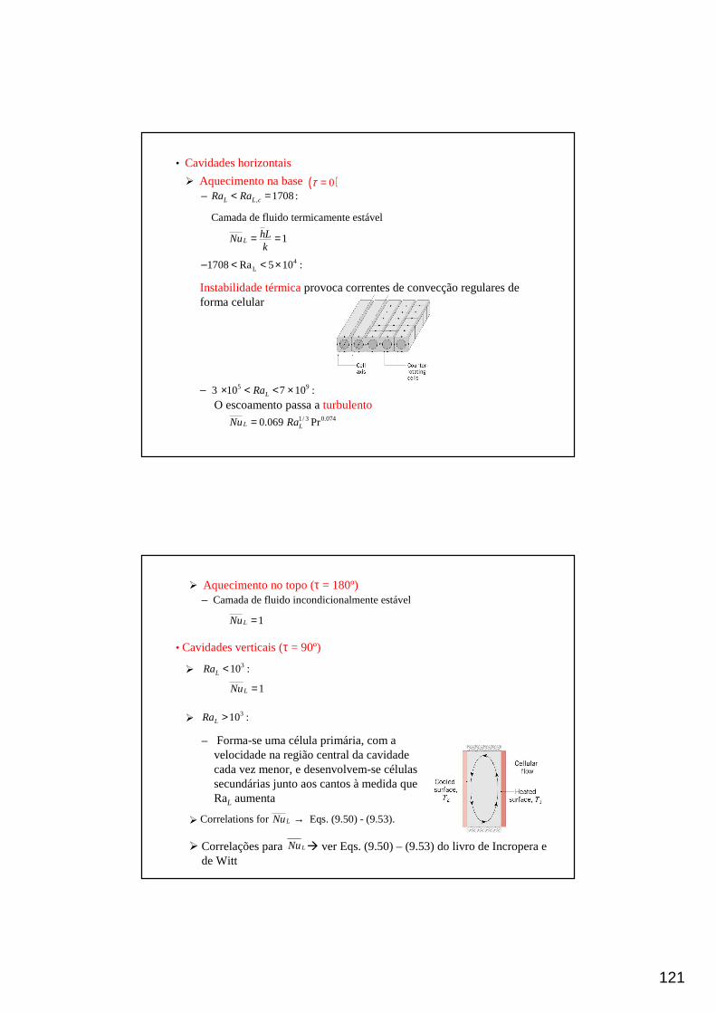
121

• Cavidades horizontais

� Aquecimento na base( )0τ =– , 1708 :L L cRa Ra< =

Camada de fluido termicamente estável

1LhLNuk

= =

– 4L1708 Ra 5 10 :< < ×

Instabilidade térmicaprovoca correntes de convecção regulares de forma celular

– 5 93 10 7 10 :LRa× < < ×O escoamento passa aturbulento

1/ 3 0.0740.069 PrL LNu Ra=

� Aquecimento no topo (τ = 180º)– Camada de fluido incondicionalmente estável

1LNu =

• Cavidades verticais (τ = 90º)

�310 :LRa <

�310 :LRa >

– Forma-se uma célula primária, com a velocidade na região central da cavidadecada vez menor, e desenvolvem-se célulassecundárias junto aos cantos à medida queRaL aumenta

� Correlations for Eqs. (9.50) - (9.53).LNu →

1LNu =

� Correlações para � ver Eqs. (9.50) – (9.53) do livro de Incropera e de Witt

LNu

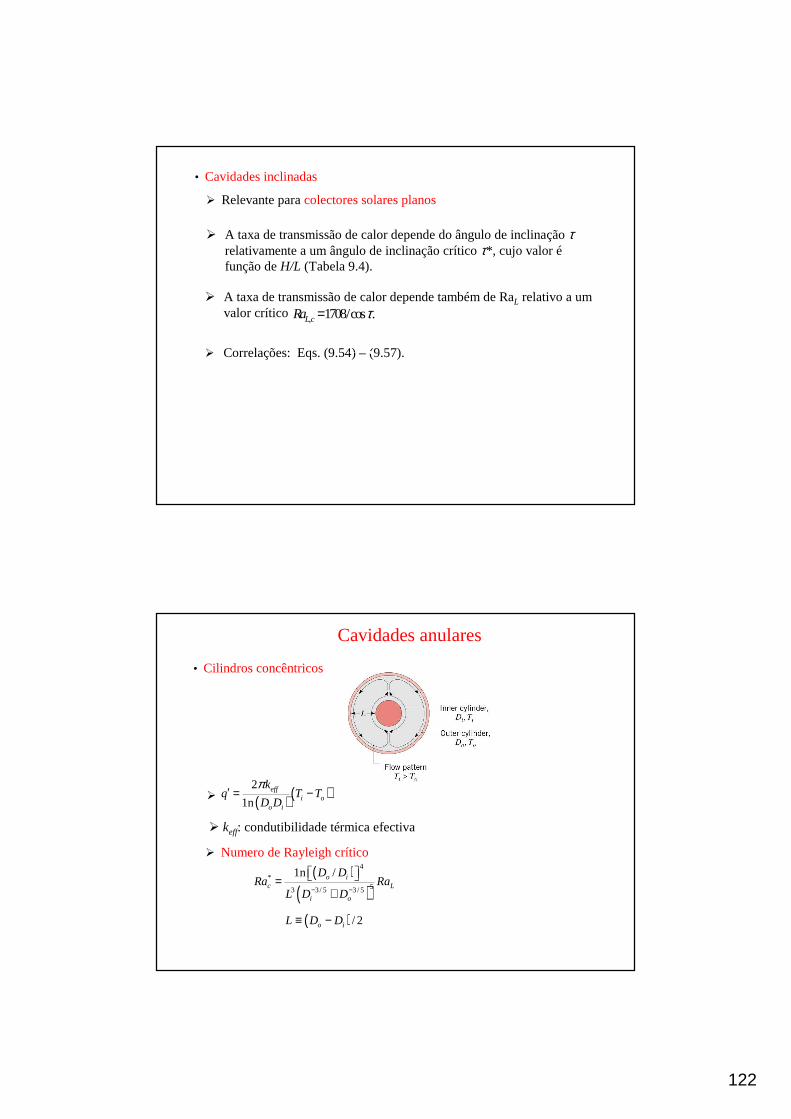
122

• Cavidades inclinadas

� Relevante paracolectores solares planos

� A taxa de transmissão de calor depende do ângulo de inclinaçãoτrelativamente a um ângulo de inclinação críticoτ*, cujo valor éfunção de H/L (Tabela 9.4).

� A taxa de transmissão de calor depende também de RaL relativo a um valor crítico

, 1708/cos .LcRa τ=

� Correlações: Eqs. (9.54) – (9.57).

Cavidades anulares

• Cilindros concêntricos

� ( ) ( )2

1neff

i oo i

kq T T

D D

π′ = −

� Numero de Rayleigh crítico:

( )( )

4

*53 3/ 5 3 / 5

1n /o ic L

i o

D DRa Ra

L D D− −

=+

( ) / 2o iL D D≡ −

� keff: condutibilidade térmica efectiva

123

�* 100 :

/ 1

c

eff

Ra

k k

<

=

�

( ) ( )

* 7

1/ 41/ 4*

100 10 :

Pr0.3860.861

c

effc

Ra

kRa

k Pr

< <

=+

• Esferas concêntricas

� ( )i oeff i o

D Dq k T T

Lπ = −

� Número de Rayleigh crítico:

( ) ( )*

4 57 / 5 7 / 5/L

s

o i i o

RaLRaD D D D− −

= +

�* 100 : / 1s effRa k k< =

�

( ) ( )

* 4

1/ 41/ 4*

100 10 :

Pr0.740.861 Pr

s

effs

Ra

kRa

k

< <

=+

• Regime misto convecção forçada – convecção natural

� Os efeitos de convecção forçada e natural são ambos importantes se

� Correlações para transmissão de calor por convecção em regime misto

n n nFC NCNu Nu Nu≈ ±

3n ≈

( ) ( )1ORe2 >>LLGr

( ) ( )1O~Re2LLGr

� O efeito de convecção natural é dominante se

� O efeito de convecção forçada é dominante se( ) ( )1ORe2 <<LLGr

+ : Força de impulsão actua no mesmo sentido ou perpendicularmente ao escoamento

- : Força de impulsão actua no sentido oposto ao do escoamento

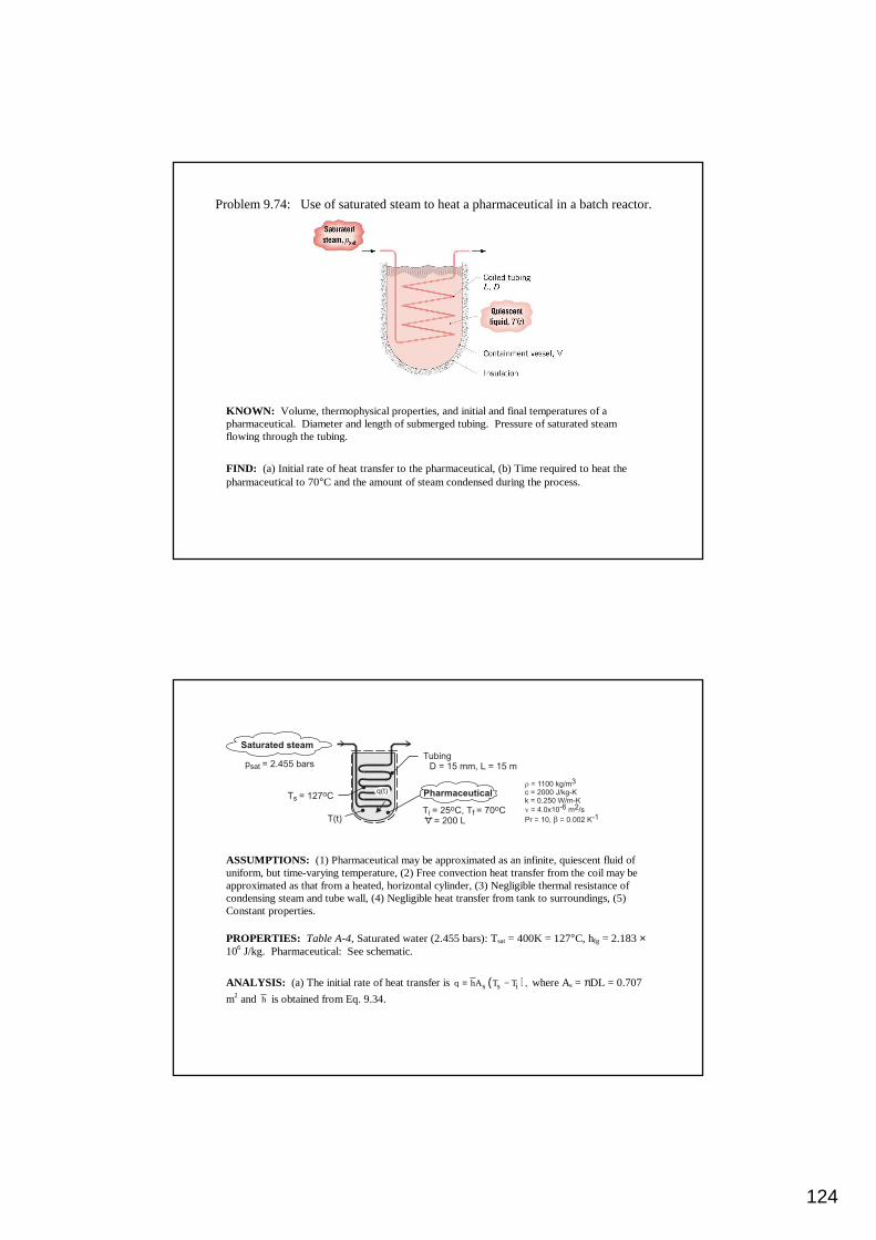
124

Problem 9.74: Use of saturated steam to heat a pharmaceutical in a batch reactor.

KNOWN: Volume, thermophysical properties, and initial and final temperatures of a pharmaceutical. Diameter and length of submerged tubing. Pressure of saturated steam flowing through the tubing.

FIND: (a) Initial rate of heat transfer to the pharmaceutical, (b) Time required to heat the pharmaceutical to 70°C and the amount of steam condensed during the process.

SCHEMATIC:

ASSUMPTIONS: (1) Pharmaceutical may be approximated as an infinite, quiescent fluid of uniform, but time-varying temperature, (2) Free convection heat transfer from the coil may be approximated as that from a heated, horizontal cylinder, (3) Negligible thermal resistance of condensing steam and tube wall, (4) Negligible heat transfer from tank to surroundings, (5) Constant properties.

PROPERTIES: Table A-4, Saturated water (2.455 bars): Tsat = 400K = 127°C, hfg = 2.183 × 106 J/kg. Pharmaceutical: See schematic.

ANALYSIS: (a) The initial rate of heat transfer is ( )s s iq hA T T ,= − where As = πDL = 0.707

m2 and h is obtained from Eq. 9.34.

125

With α = ν/Pr = 4.0 × 10-7 m2/s and RaD = gβ (Ts – Ti) D3/αν = 9.8 m/s2 (0.002 K-1) (102K)

(0.015m)3/16 × 10-13 m4/s2 = 4.22 × 106,

( )

( )( )

D

2 21/ 661/ 6

D8 / 27 8 / 279 /16 9 /16

0.387 4.22 100.387 RaNu 0.60 0.60 27.7

1 0.559 / Pr 1 0.559 /10

×

= + = + = + +

Hence, 2Dh Nu k / D 27.7 0.250 W / m K / 0.015m 462 W / m K= = × ⋅ = ⋅

and ( ) ( )2 2s s iq hA T T 462W / m K 0.707 m 102 C 33,300 W= − = ⋅ × ° =

(b) Performing an energy balance at an instant of time for a control surface about the liquid,

( ) ( ) ( ) ( )( )s s

d cTq t h t A T T t

dt

ρ∀= = −

where the Rayleigh number, and hence h, changes with time due to the change in the temperature of the liquid.

Integrating the foregoing equation numerically, the following results are obtained for the variation of T and h with t.

0 100 200 300 400 500 600 700 800 900

Time, t(s)

25

35

45

55

65

75

Tem

pera

ture

, (C

)

0 100 200 300 400 500 600 700 800 900

Time, t(s)

370

390

410

430

450

470

Con

vect

ion

coef

ficie

nt, h

bar

(W/m

^2.K

)

The time at which the liquid reaches 70°C is ft 855s≈ <

The rate at which T increases decreases with increasing time due to the corresponding reduction in (Ts – T), and hence reductions in DRa , h and q.

The Rayleigh number decreases from 4.22 × 106 to 2.16 × 106, while the heat rate decreases from 33,300 to 14,000 W.

The convection coefficient decreases approximately as (Ts – T)1/3, while q ~ (Ts – T)4/3.

126

The latent energy released by the condensed steam corresponds to the increase in thermal energy of the pharmaceutical. Hence, c fgm h = ( )f ic T T ,ρ∀ −

and

( ) 3 3

f ic 6fg

c T T 1100 kg / m 0.2m 2000 J / kg K 45 Cm 9.07 kg

h 2.183 10 J / kg

ρ∀ − × × ⋅ × °= = =×

<

COMMENTS: (1) Over such a large temperature range, the fluid properties are likely to vary significantly, particularly ν and Pr. A more accurate solution could therefore be performed if the temperature dependence of the properties were known. (2) Condensation of the steam is a significant process expense, which is linked to the equipment (capital) and energy (operating) costs associated with steam production.

Heat Exchangers:Heat Exchangers:Design ConsiderationsDesign Considerations

127

Heat Exchanger Types

Heat exchangers are ubiquitous to energy conversion and utilization. They involve heat exchange between two fluids separated by a solid and encompass a wide range of flow configurations.

• Concentric-Tube Heat Exchangers

Parallel Flow Counterflow

� Simplest configuration.

� Superior performance associated with counter flow.

• Cross-flow Heat Exchangers

Finned-Both FluidsUnmixed

Unfinned-One Fluid Mixedthe Other Unmixed

� For cross-flow over the tubes, fluid motion, and hence mixing, in the transversedirection (y) is prevented for the finned tubes, but occurs for the unfinned condition.

� Heat exchanger performance is influenced by mixing.

128

• Shell-and-Tube Heat Exchangers

One Shell Pass and One Tube Pass

� Bafflesare used to establish a cross-flow and to induce turbulent mixing of theshell-side fluid, both of which enhance convection.

� The number of tube and shell passes may be varied, e.g.:

One Shell Pass,Two Tube Passes

Two Shell Passes,Four Tube Passes

• Compact Heat Exchangers

� Widely used to achievelarge heat rates per unit volume, particularly when one or both fluids is a gas.

� Characterized bylarge heat transfer surface areas per unit volume, small flow passages, and laminar flow.

(a) Fin-tube (flat tubes, continuous plate fins)(b) Fin-tube (circular tubes, continuous plate fins)(c) Fin-tube (circular tubes, circular fins)(d) Plate-fin (single pass)(e) Plate-fin (multipass)

129

Overall Heat Transfer Coefficient• An essential requirement for heat exchanger design or performance calculations.

• Contributing factors includeconvectionandconductionassociated with thetwo fluids and the intermediate solid, as well as the potential use offins on bothsides and the effects of time-dependent surfacefouling.

• With subscriptsc andh used to designate thehot andcold fluids, respectively,the most general expression for the overall coefficient is:

( ) ( )

( ) ( ) ( ) ( ), ,

1 1 1

1 1

c h

f c f hw

o o o oc c h h

UA UA UA

R RR

hA A A hAη η η η

= =

′′ ′′= + + + +

�

( )o,

Overall surface efficiency of fin array (Section 3.6.5)

1 1

o

fc or h f

c or h

A

A

η

η η

→ = − −

total surface area (fins and exposed base) surface area of fins only

t

f

A AA

= →→

Assuming an adiabatic tip, thefin efficiencyis

( ),

tanhf c or h

c or h

mL

mLη =

( )2 /c or h p w c or hm U k t=

, partial overall coe1

fficientp c or hf c or h

hUhR

= → ′′+

�2 for a unit surFouling fa face area (ctor m K/W)fR′′ → ⋅

Table 11.1→

conduction resistan Wall (K/Wce ) wR →�

130

A Methodology for Heat ExchangerDesign Calculations

- The Log Mean Temperature Difference (LMTD) Method -• A form of Newton’s Law of Cooling may be applied to heat exchangers by

using a log-mean value of the temperature difference between the two fluids:

1mq U A T∆=

( )1 2

11 21n /m

T TT

T T∆ ∆∆

∆ ∆−=

Evaluation of depends on the heat exchanger type.1 2 and T T∆ ∆

• Counter-Flow Heat Exchanger:

1 ,1 ,1

, ,

h c

h i c o

T T TT T

∆ ≡ −= −

2 ,2 ,2

, ,

h c

h o c i

T T TT T

∆ ≡ −= −

• Parallel-Flow Heat Exchanger:

1 ,1 ,1

, ,

h c

h i c i

T T TT T

∆ ≡ −= −

2 ,2 ,2

, ,

h c

h o c o

T T TT T

∆ ≡ −= −

� Note that Tc,o can not exceed Th,o for a PF HX, but can do so for a CF HX.

� For equivalent values of UA and inlet temperatures,

1 , 1 ,m CF m PFT T∆ ∆>

• Shell-and-Tube and Cross-Flow Heat Exchangers:

1 1 ,m m CFT F T∆ ∆=

Figures 11.10 - 11.13F →

132

Overall Energy Balance

• Assume negligible heat transfer between the exchanger and its surroundingsand negligible potential and kinetic energy changes for each fluid.

( ), ,h i h ohq m i i⋅= −

( ), ,c c o c iq m i i⋅= − fluid enthalpyi →

• Assuming no l/v phase change and constant specific heats,

( ), , ,p h h i h ohq m c T T⋅= − ( ), ,h h i h oC T T= −

( ), , ,c p c c o c iq m c T T⋅

= − ( ), ,c c o c iC T T= −

, Heat capacity r s ateh cC C →

• Application to the hot (h)and cold (c)fluids:

Special Operating Conditions

� Case (a): Ch>>C c or h is a condensing vapor( ).hC → ∞

– Negligible or no change in ( ), , .h h o h iT T T=

� Case (b): Cc>>C h or c is an evaporating liquid( ).cC → ∞

– Negligible or no change in ( ), , .c c o c iT T T=

� Case (c): Ch=Cc.

1 2 1mT T T∆ ∆ ∆= =–

133

Heat Exchangers:Heat Exchangers:The Effectiveness The Effectiveness –– NTU MethodNTU Method

General Considerations

• Computational Features/Limitations of the LMTD Method:

� The LMTD method may be applied todesign problemsfor which the fluid flow rates and inlet temperatures, as well as a desired outlet temperature, are prescribed.For a specifiedHX type, the required size (surface area), as well as the other outlet temperature, are readily determined.

� If the LMTD method is used inperformance calculationsfor whichboth outlet temperatures must be determined from knowledge of theinlet temperatures, the solution procedure is iterative.

� For both design and performance calculations, the effectiveness-NTUmethod may be used without iteration.

134

DefinitionsDefinitions

Definitions• Heat exchangereffectiveness, : ε

max

qq

ε =

0 1ε≤ ≤

• Maximumpossibleheat rate:

( )max min , ,h i c iq C T T= −

min

if or

h h cC C CC

<= if c c hC C C<

� Will the fluid characterized by Cmin or Cmaxexperience the largest possibletemperature change in transit through the HX?

� Why is Cmin and not Cmaxused in the definition of qmax?

• Number of Transfer Units, NTU

min

UANTUC

≡

� A dimensionless parameter whose magnitude influences HX performance:

with q NTU↑ ↑

135

Heat Exchanger Relations

( )( )

, ,

, ,

h i h oh

h h i h o

q m i ior

q C T T

⋅ = − = −

•

•( )( )

, ,

, ,

c c o c i

c c o c i

q m i ior

q C T T

⋅ = − = −

• ( )min , ,h i c iq C T Tε= −

• Performance Calculations:� ( )min max, /f NTU C Cε =

Cr

� Relations Table 11.3 or Figs. 11.14 - 11.19→

ε-NTU Expressions (Table 2.2 of the book, more detail in book)

1 to 2 shell-and-tube HEX

Cross flow, Cmaxmixed and Cminunmixed

Cross flow, Cminmixed and Cmaxunmixed

Parallel Flow

Counterflow

NTU(ε,C*)ε(NTU,C*)Type of HEX

1 to 2 shell-and-tube HEX

Cross flow, Cmaxmixed and Cminunmixed

Cross flow, Cminmixed and Cmaxunmixed

Parallel Flow

Counterflow

NTU(ε,C*)ε(NTU,C*)Type of HEX

( )[ ]( )[ ]NTU1exp1

NTU1exp1

∗−−

∗−

∗−−−

=CC

Cε

−

∗−

∗−

=ε

ε

1

1ln

1

1NTU

C

C

( )[ ][ ]NTU1exp11

1 ∗+−−∗

+= C

Cε

( )

∗

∗−−

−=C

C NTUexp1exp1ε

( )[ ]{ }[ ]NTUexp1exp11

−−∗

−−∗= CC

ε

( )

∗+−−

∗+−+∗

++∗

+

=

2/121NTUexp1

2/121NTUexp1

2/1211

2

C

C

CC

ε

( )[ ]∗++∗

+−= C

C11ln

1

1NTU ε

( )[ ]ε−∗

+∗−= 1ln1ln1

NTU CC

( )

∗−∗+= C

Cε1ln

11-lnNTU

( )

∗++∗+−

∗+−∗+−

∗+

=2/1

2112

2/12112

ln2/12

1

1NTU

CC

CC

C ε

ε

137

• Design Calculations:

� ( )min max, /NTU f C Cε=

� Relations Table 11.4 or Figs. 11.14 - 11.19→

• For all heat exchangers,

with rCε ↑ ↓

( )1 exp NTUε = − −

( )

or

1n 1NTU ε= − −

• For Cr = 0, to all HX types.a single relation appliesNTUε −

Radiação: Considerações gerais

• Estuda-se radiação térmica, cujas origens estão ligadas àemissãoda matéria a uma temperatura absoluta T>0

• A emissão édevida oscilações e transições electrónicas dosmuitoselectrõesqueconstituem a matéria que, por sua vez, são mantidos pela energia térmica da matéria

• A emissão correspondeà energia transferida da matéria (calor) e, portanto, correspondeà redução de energia térmica armazenada na matéria.

• A radiação também pode serintersectada e absorvidapela matéria.

• A absorção resulta emtransferência de calor para a matéria e, portanto, corresponde a um amento de energia térmica armazenada na matéria.

• Considere um sólido à temperatura Tsnum recinto fechado com vácuo, cujas paredes estão à temperatura Tsur

� Que fenómeno ocorre se Ts > Tsur? Porquê

� Que fenómeno ocorre se Ts < Tsur? Porquê

138

• A emissão de gases ou sólidos semi-transparentes ou líquidos é um fenómeno volumétrico. •A emissão de sólidos ou líquidos opacos é um fenómeno superficial (com a emissão originária em átomos ou moléculas a 1 µm da superfície).

• A natureza dual da radiação:– Nalguns casos, as manifestações físicas da radiação podem ser explicadas

olhando-as como partículas(akafotõesou quanta).

– Noutros casos, a radiação comporta-se como umaonda electromagnética.


cλν

=

8 2 998 10 m/soc c= = . x

Em qualquer dos casos, a radiação é caracterizada por um comprimento de onda λe frequência υ que estão relacionados pela velocidade de propagação da radiação no meio em causa, c:

No vácuo:

O espectro electromagnético


139

A quantidade de radiação emitida por uma superfície opaca varia com o comprimento de onda, podendo falar-se em distribuição espectral em todos os comprimentos de onda ou de componentes monocromáticas/espectraisassociadas a comprimentos de onda específicos.


Efeitos direccionais

A radiação emitida por uma superfície sê-lo-á em todas as direcções do hemisfério e segundo uma distribuição direccional

A direcção pode ser representada em coordenadas esféricas peloângulo polar ou zenital θ e pelo ângulo azimutal ϕ.


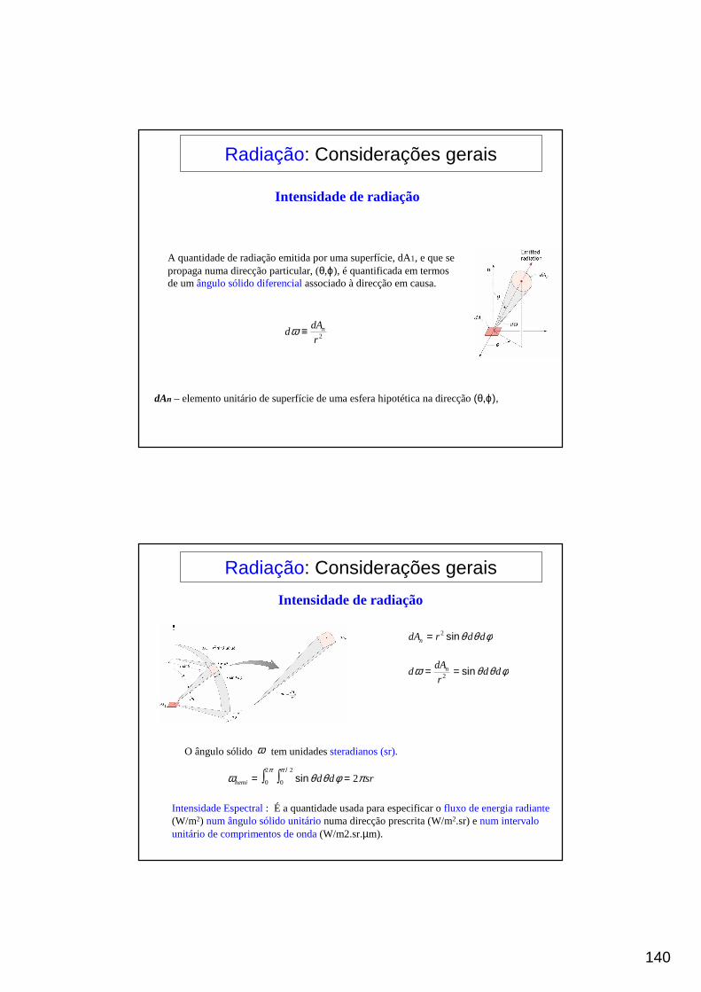
140

Intensidade de radiação

A quantidade de radiação emitida por uma superfície, dA1, e que sepropaga numa direcção particular, (θ,ϕ), é quantificada em termosde um ângulo sólido diferencialassociado à direcção em causa.

2ndA

dr

ω ≡

dAn – elemento unitário de superfície de uma esfera hipotética na direcção (θ,ϕ),




2ndA r d dθ θ φ= sin

2ndA

d d dr

ω θ θ φ= = sin

O ângulo sólido tem unidades steradianos (sr).ω

2 2

0 0 2hemi d d srπ π

ω θ θ φ π= =∫ ∫/

sin

Intensidade Espectral: É a quantidade usada para especificar o fluxo de energia radiante(W/m2) num ângulo sólido unitárionuma direcção prescrita (W/m2.sr) e num intervalounitário de comprimentos de onda(W/m2.sr.µm).

141



( ) ( )1e

dqI

dA d dλ λ θ φθ ω λ

≡⋅ ⋅, , ,

cos

A intensidade espectral, , associada à emissão de um elemento de área unitário, ,num ângulo sólido, (em torno de θ e φ),e num intervalo de comprimento de onda, , (em torno de ), é:

eI λ , 1dAdω dλ

λ

eI λ ,

O argumento para definir o fluxo radiativo em termos da área projectada da superfícieemerge do facto de haver superfícies para as quais, com boa aproximação,

é independente da direcção: superfícies difusas,e a radiação éisotrópica.( )1dA θcos

A área projectada é como apareceriaSe observada segundo os ângulos

1dAθ φ,

– Quanto vale a área projectada para ?0θ =

– Quanto vale a área projectada para ?2θ π= /



( ) 1edq

dq I dA ddλ λ λ θ φ θ ω

λ≡ = , , , cos

A taxa de calor espectral e o fluxo de calor espectral associados à emissão a partir de são, respectivamente,

1dA

( ) ( )e edq I d I d dλ λ λλ θ φ θ ω λ θ φ θ θ θ φ′′ = =, ,, , cos , , cos sin

142

Relação da intensidade com poder emissivo, irradiação e radiosidade

( ) ( )2 2

0 0 eE I d dπ π

λ λλ λ θ φ θ θ θ φ= ∫ ∫/

, , , cos sin

( )0E E dλ λ λ∞

= ∫

( ) ( )eE Iλ λλ π λ= ,

O poder emissivo espectral(W/m2.µm) corresponde à emissão espectral em todas as direcções possíveis:

eE Iπ=

O poder emissivo total(W/m2) corresponde à emissão espectral em todas as direcções e comprimentos de onda possíveis:

Para superfícies difusas, a emissão é isotrópicae:

A intensidade espectral da radiação incidente numa superfície, é definida em termos do ângulo sólido unitário em torno dadirecção de incidência, do intervalo de comprimento de onda, em torno de, , e da área projectada do receptor,

iIλ ,

dλλ 1dA θcos .


( ) ( )2 2

0 0 iG I d dπ π

λ λλ λ θ φ θ θ θ φ= ∫ ∫/

, , , cos sin

( )0G G dλ λ λ∞

= ∫

A irradiação espectral vale:( )2W/m mµ⋅

e a irradiação totalé : ( )2W/m

� Quantos e G são expressos se a radiação for difusa?Gλ

A radiosidadede uma superfície opaca contabilizatoda a radiação que abandona a superfície em todasas direcções e pode incluir as contribuições dareflexão e emissão.

143


( ) ( )2 2

0 0 e rJ I d dπ π

λ λλ λ θ φ θ θ θ φ+= ∫ ∫/

, , , cos sin

( )0J J dλ λ λ∞

= ∫

Com a designar a intensidade espectral associada à radiação emitida pela superfície e a reflexão da radiação incidente, a radiosidade espectral é :

e rIλ +,

( )2W/m mµ⋅

E a radiosidade totalé :( )2W/m

� Quantos e J podem ser expressos se a superfície emitir e reflectir de forma difusa?Jλ

Radiação de CORPO NEGRO

• O Corpo Negro

� Umaidealizaçãoque fornece oslimites daradiação emitida e absorvidapela matéria.

– Para uma dada temperatura e um dado comprimento de onda, nenhuma superfície é capaz de emitir mais que um corpo negro: emissorideal.

– Um corpo negro é um emissor difuso.

– Um corpo negro absorve toda a radiação incidente: absorvedor ideal.

144

Radiação de CORPO NEGRO• A Cavidade Isotérmica(Hohlraum):parede interior a temperatura uniforme.

(a) Depois de múltiplas reflexões, toda a radiação entrada na cavidade évirtualmenteabsorvida⇒ corpo negro.

(b) A emissãoa partir da abertura é a máximaque se pode atingir, para atemperaturaassociada àcavidade,e édifusa (independente da direcção) ⇒⇒ corpo negro.

(c) O campo radiativo no interior da cavidade (efeito acumulado da radiação emitidae da reflectida pelaparede da cavidade) tem por efeito assegurar uma irradiaçãodifusa (correspondente à emissão de um corpo negro numa forma igual à radiação emergentepela abertura). O campo radiativo no interior da cavidade é de corpo negro. Qualquer superfície no interior da cavidade é irradiada de forma difusa: ( )bG Eλ λ= ,

– Esta condição depende da superfície da cavidade ser acentuadamentereflectora ou absorvedora?

Lei da distribuição de Plank

3 2898 m KT Cλ µ= = ⋅max

( ) ( ) ( )1

52 1b b

CE T I T

C Tλ λλ π λλ λ

= =−

, ,, ,exp /

• A distribuição espectral do poder emissivo de um corpo negro(determinado teoricamentee confirmado experimentalmente) é (Plank):

Primeira constante: 8 4 2

1 3 742 10 W m mC µ= ⋅. x /

Segunda constante: 42 1 439 10 m KC µ= ⋅. x

� varia continuamente com e aumenta com T. bEλ , λ

� A distribuição é caracterizada por um máximo para o qual édado pelalei deslocamento de Wien:

λmax

� A quantidade fraccionalda emissão total de corpo negroque aparece a baixoscomprimentos de onda aumenta com o aumento de T.

145

Lei de Stefan-Boltzmann

( ) ( ) ( )

2 1

1 2 2 1

00 0 4

b o bE d E dF F F

T

λ λλ λ

λ λ λ λλ λσ− − −

∫ − ∫= − = , ,

( ) ( )00

bE dF f T

T

λλ

λλ

λσ−

∫= =,

• O poder emissivo totalde um corpo negro é obtido integrando a distribuição de Planck em todos os comprimentos de onda possíveis.

40b b bE I E d Tλπ λ σ∞

= = =∫ ,

a lei de Stefan-Boltzmann, em que:

Kσ −

σ é a constante se Stefan-Boltzmann,σ = 5,670 × 10-8 W/m2.K4

• A fracção total daemissãode um corpo negro que está contidanum intervalo de comprimentode onda prescritoou banda é:( )1 2λ λ λ< <

Lei de Stefan-Boltzmann – fracção de energia

Kσ −

( ) ( ) ( )1

52 1b b

CE T I T

C Tλ λλ π λλ λ

= =−

, ,, ,exp /

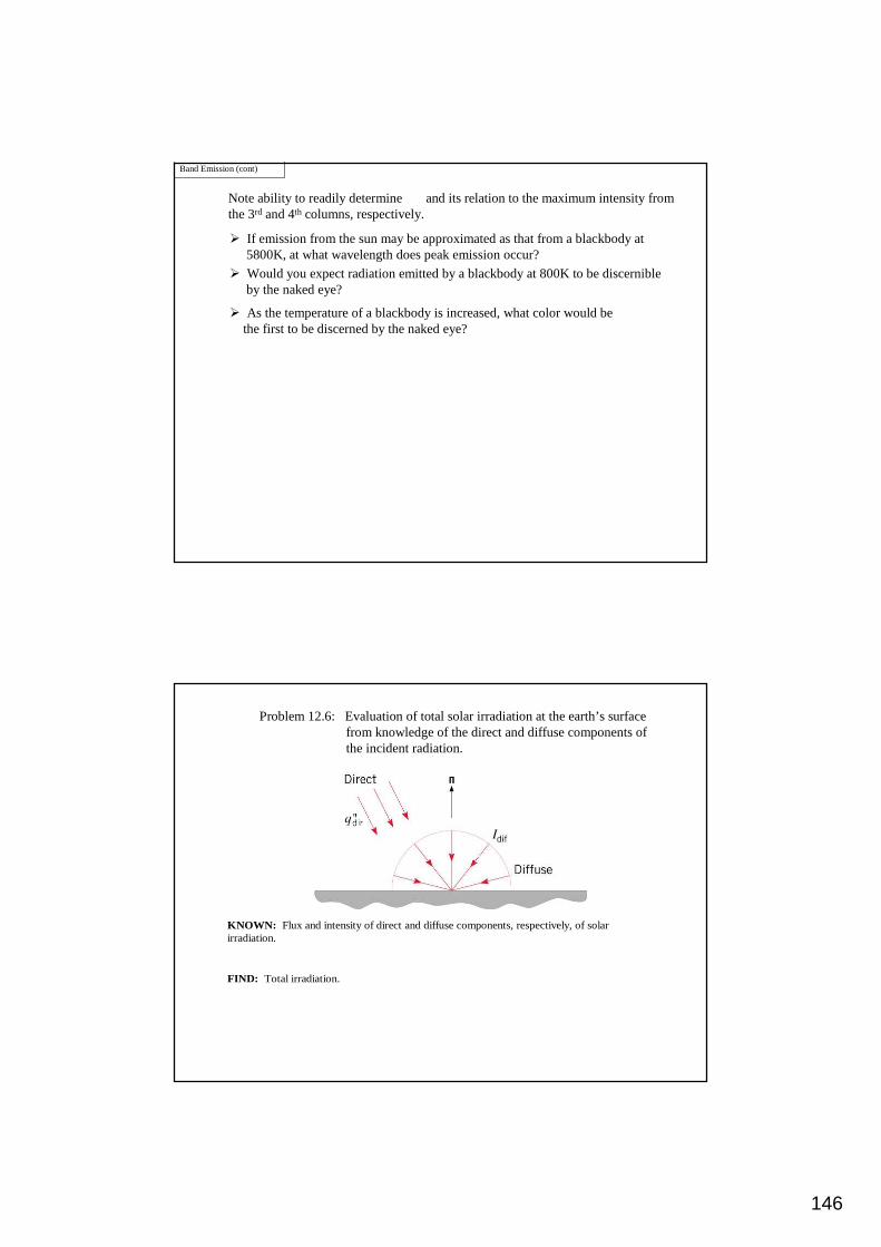
146

Band Emission (cont)

Note ability to readily determine and its relation to the maximum intensity fromthe 3rd and 4th columns, respectively.

bI λ ,

� If emission from the sun may be approximated as that from a blackbody at5800K, at what wavelength does peak emission occur?

� Would you expect radiation emitted by a blackbody at 800K to be discernibleby the naked eye?

� As the temperature of a blackbody is increased, what color would bethe first to be discerned by the naked eye?

Problem 12.6: Evaluation of total solar irradiation at the earth’s surfacefrom knowledge of the direct and diffuse components of the incident radiation.

KNOWN: Flux and intensity of direct and diffuse components, respectively, of solar irradiation.

FIND: Total irradiation.

147

SCHEMATIC:

ANALYSIS: Since the irradiation is based on the actual surface area, the contribution due to the direct solar radiation is dir dirG q cos .θ′′= ⋅

For the contribution due to the diffuse radiation dif difG I .π=

Hence dir dif dir difG G G q cos Iθ π′′= + = ⋅ +

or

2 2G 1000 W / m 0.866 sr 70W / m srπ= × + × ⋅

( ) 2G 866 220 W / m= +

2G 1086 W / m .=

COMMENTS: Although a diffuse approximation is often made for the non-direct component of solar radiation, the actual directional distribution deviates from this condition, providing larger intensities at angles close to the direct beam.

148

Problem 12.18: Determination of the sun’s emissive power, temperatureand wavelength of maximum emission, as well as theearth’s temperature, from knowledge of the sun/earthgeometry and the solar flux at the outer edge of the earth’satmosphere.

KNOWN: Solar flux at outer edge of earth’s atmosphere, 1353 W/m2.

FIND: (a) Emissive power of sun, (b) Surface temperature of sun, (c) Wavelength of maximum solar emission, (d) Earth equilibrium temperature.

SCHEMATIC:

ASSUMPTIONS: (1) Sun and earth emit as blackbodies, (2) No attenuation of solar radiation enroute to earth, (3) Earth atmosphere has no effect on earth energy balance.

ANALYSIS: (a) Applying conservation of energy to the solar energy crossing two concentric spheres, one having the radius of the sun and the other having the radial distance from the edge of the earth’s atmosphere to the center of the sun, it follows that

( ) s

22 e

s s s eD

E D 4 R q .2

π π − ′′= −

Hence

( )

( )

211 7 27 2

s 29

4 1.5 10 m 0.65 10 m 1353 W / mE 6.302 10 W / m .

1.39 10 m

× − × ×= = ×

×

(b) From the Stefan-Boltzmann law, the temperature of the sun is

1/ 41/ 4 7 2s

s 8 2 4

E 6.302 10 W / mT 5774 K.

5.67 10 W / m Kσ −

× = = = × ⋅

(c) From Wien’s law, the wavelength of maximum emission is

3max

C 2897.6 m K0.50 m.

T 5774 K

µλ µ⋅= = =

149

Hence, from the Stefan-Boltzmann law,

S1/ 41/ 4 2

e 8 2 4

q 1353 W / mT 278 K.

4 4 5.67 10 W / m Kσ −

′′ = = = × × ⋅

COMMENTS: The average earth temperature is higher than 278 K due to the shielding effect of the earth’s atmosphere (transparent to solar radiation but not to longer wavelength earth emission).

(d) From an energy balance on the earth’s surface

( ) ( )2 2e e S eE D q D / 4 .π π′′=

Processos e propriedades radiativas. Propriedades radiativas de superfícies

( ) ( )( )

e

b

I TT

I Tλ

λ θλ

λ θ φε λ θ φ

λ≡ ,

,,

, , ,, , ,

,

( ) ( )( )

( )( )

2 20 0

2 20 0

e

b b

I T d dE TT

E T I T d d

π πλλ

λ π πλ λ

λ θ φ θ θ θ φλε λλ λ θ θ θ φ

∫ ∫≡ =

∫ ∫

/,

/, ,

, , , cos sin,,

, , cos sin

Emissividade de uma SuperfícieIntroduzindo uma propriedade específica, (a emissividade), a radiação emitida por uma superfície pode ser determinada, o que contrasta com o seu comportamento ideal como corpo negro à mesma temperatura.A definição de emissividadedepende de estarmos interessados em calcular o carácter direccional e/ou espectralda radiação emitida, em contraste com médias em todas as direcções (radiação hemisférica)e/ou em todos os comprimentos de onda (total).

• A emissividade espectral directional:

• A emissividade espectral hemisférica(uma média direccional):

150


( ) ( )( )

( ) ( )( )

0 b

b b

T E T dE TT

E T E Tλ λε λ λ λ

ε∞∫

≡ = ,, , ,

• A emissividade total hemisférica(uma média direccional e espectral):

Valores típicos da emissividade total normal :

Notas:� Baixas emissividades dos metais polidos e crescente emissividade de metais não polidose superfícies oxidadas.

� Emissividades comparativamente elevadasdos não condutores.

Com um boa de aproximação, a emissividade hemisférica é igual à emissividade normal:nε ε=


• Variações espectrais típicas

Notar decréscimo de com o aumento de para metaise comportamento diferente dos não metais

nλε ,

λ

• Variações de temperatura típicas:

Porque é que aumenta com o aumento de para o tungsténio e não aumenta para o óxido de alumínio?

nε λ

151

ref abs trG G G Gλ λ λ λ= + +, , ,

Absorção, reflexão e transmissão: resposta à radiação incidente

ref abs trG G G Gλ λ λ λ= + +, , ,

• Pode haver 3 respostas de um meio semi transparenteà irradiação:

� Reflexãopelo meio( )refGλ , .

� Absorçãopelo meio ( )absGλ , .

� Transmissãoatravés do meio( )trGλ , .

Balanço de Radiação

O comprimento de ondadaradiação incidentee a natureza do materialdeterminam se o material ésemitransparenteouopaco.

� O vidro e a águasãosemitransparentesou opacos?

• Contrastando com o que se disse para meios semitransparentes, efeitos volumétricos, a resposta de um material opacoà irradiação é governado porfenómenos superficiaise 0trGλ =, .

Absorção, reflexão e transmissão: resposta à radiação incidente

• A menos que um material opaco esteja a uma temperatura suficientemente alta para emitirradiação visível, a suacor é determinada pela dependência espectral da reflexão em respostaà irradiação visível.

� O que se pode dizer sobre a reflexão de uma superfíciebranca?� E sobre umanegra?

� Porque é que as folhas sãoverdes?

152

Absorsividade de uma superfície opaca

( ) ( )( )

i abs

i

I

Iλ

λ θλ

λ θ φα λ θ φ

λ θ φ≡ , ,

,,

, ,, ,

, ,

( ) ( )( )

( ) ( )( )

2 20 0

2 20 0

abs i

i

G I d d

G I d d

π πλ λ θ λ

λ π πλ λ

λ α λ θ φ λ θ φ θ θ θ φα λ

λ λ θ φ θ θ θ φ∫ ∫

≡ =∫ ∫

/, , ,

/,

, , , , cos sin

, , cos sin

• A absorsividade espectral hemisférica:

� Se a radiação for difusa, em que é que se simplifica o resultado anterior?

E se a superfície for difusa?

• A absorsividade total hemisférica:

� Se a irradiação for de corpo negro, como se escrevem as equações anteriores?

• A absorsividade espectral direccional, desprezando dependência de T:

� A absorsividade é aproximadamente independente da temperatura da superfície, mas se a irradiação for de corpo negro, porque é que depende da temperaturado corpo negro?

α

( ) ( )( )0

oabs G dG

G G dλ λ

λ

α λ λ λαλ λ

∞

∞∫

≡ =∫

Reflectividade de uma superfície opaca

( ) ( )( )

i ref

i

I

Iλ

λ θλ

λ θ φρ λ θ φ

λ θ φ≡ , ,

,

,

, ,, ,

, ,

( )( )

( ) ( )( )

220 0ref i

i

G I d d

G I

ππλ λ θ λ

λλ λ

λ ρ λ θ φ λ θ φ θ θ θ φρλ λ θ φ

∫ ∫≡ =

/

, , ,

,

, , , , cos sin

, ,

( ) ( )( )

0

0

abs G dG

G G dλ λ

λ

ρ λ λ λρλ λ

∞

∞∫

≡ =∫

• A absorsividade espectral hemisférica:

� Se a radiação for difusa, em que é que se simplifica o resultado anterior?

E se a superfície for difusa?

• A reflectividade total hemisférica:

• A reflectividade espectral direccional, desprezando dependência de T:

• Condições limitativas de reflexão difusa eespectral. Superfícies polidas e rugosas.

153

� Notar forte dependência de ρλ (e αλ = 1- ρλ) emλ

Reflectividade de uma superfície opaca

� A neve é uma substância muito reflectora?E a tinta branca?

Transmissividade

( )trG

Gλ

λλ

λτ

λ≡ ,

( )( )

0

0

trtr G dG

G G dλ

λ

λ λτ

λ λ

∞

∞∫

≡ =∫

,• A reflectividade total hemisférica:

• A transmissividade espectral hemisférica ,desprezando dependência de T:

Notar que a pequenos e elevados comprimentos de onda há mudança de condições de semitransparente para opaco

• Para um meio semitransparente,

1

1

=++=++

ταρταρ λλλ • Para um meio opaco,

1

1

=+=+

αραρ λλ

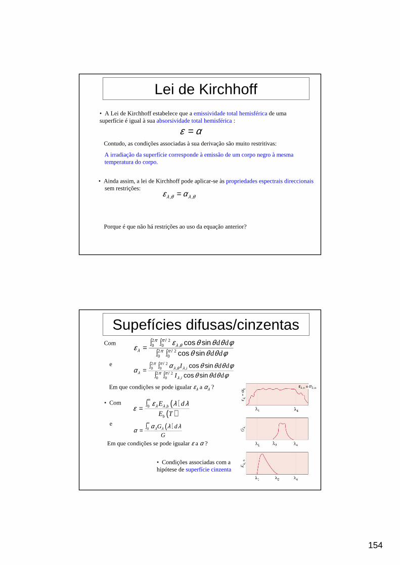
154

Lei de Kirchhoff

ε α=

• A Lei de Kirchhoff estabelece que a emissividade total hemisféricade umasuperfície é igual à suaabsorsividade total hemisférica:

Contudo, as condições associadas à sua derivação são muito restritivas:

A irradiação da superfície corresponde à emissão de um corpo negro à mesmatemperatura do corpo.

• Ainda assim, a lei de Kirchhoff pode aplicar-se àspropriedades espectrais direccionaissem restrições:

Porque é que não há restrições ao uso da equação anterior?

λ θ λ θε α=, ,

Supefícies difusas/cinzentasCom 2 2

0 02 20 0

d d

d d

π πλ θ

λ π πε θ θ θ φ

εθ θ θ φ

∫ ∫=

∫ ∫

/,

/

cos sin

cos sine 2 2

0 02 20 0

i

i

I d d

I d d

π πλ θ λ

λ π πλ

α θ θ θ φα

θ θ θ φ∫ ∫

=∫ ∫

/, ,

/,

cos sin

cos sin

Em que condições se pode igualarελ a αλ ?

• Com ( )( )

0 b

b

E d

E Tλ λε λ λ

ε∞∫

= ,

e ( )0 G d

Gλ λα λ λα

∞∫

=

Em que condições se pode igualarε a α ?

• Condições associadas com ahipótese de superfície cinzenta

155

Problem 12.49: Determination of the solar absorptivity and total emissivityof a diffuse surface from knowledge of the spectraldistribution of and the surface temperature.( )λα λ

KNOWN: Spectral, hemispherical absorptivity of an opaque surface.

FIND: (a) Solar absorptivity, (b) Total, hemispherical emissivity for Ts = 340K.

SCHEMATIC:

ASSUMPTIONS: (1) Surface is opaque, (2) ελ = αλ, (3) Solar spectrum has Gλ = Gλ,S proportional to Eλ,b (λ, 5800K).

ANALYSIS: (a) The solar absorptivity may be expressed as

( ) ( ) ( )S ,b ,b0 0E ,5800K d / E ,5800K d .λ λ λα α λ λ λ λ λ∞ ∞

= ∫ ∫

The integral can be written in three parts using F(0 → λ) terms.

( ) ( ) ( ) ( )S 1 2 30 0.3 0 1.5 0 0.3 0 1.5F F F 1 F .α α α α→ → → → = + − + −

From Table 12.1, λT = 0.3 × 5800 = 1740 µm⋅K F(0 → 0.3 µm) = 0.0335 λT = 1.5 × 5800 = 8700 µm⋅K F(0 → 1.5 µm) = 0.8805.

156

Hence, [ ] [ ]S 0 0.0355 0.9 0.8805 0.0335 0.1 1 0.8805 0.774.α = × + − + − =

(b) The total, hemispherical emissivity for the surface at 340K may be expressed as

( ) ( ) ( ),b b0E ,340K d / E 340K .λ λε ε λ λ λ∞

= ∫

With ελ = αλ, the integral can be written in terms of the F(0 → λ) function. However, it is readily recognized that since ( )0 1.5 m,340KF 0.000 at T 1.5 340 510 m Kµ λ µ→ ≈ = × = ⋅ there is negligible emission below 1.5 µm.

It follows that 0.1λ λε ε α= = =

COMMENTS: The assumption ελ = αλ is satisfied if the surface is irradiated diffusely or if the surface itself is diffuse. Note that for this surface under the specified conditions of solar irradiation and surface temperature, αS ≠ ε. Such a surface is spectrally selective.

Problem 12.90: Determination of the emissivity and absorptivity of a coatedvertical plate exposed to solar-simulation lamps and the magnitudeof the irradiation required to maintain a prescribed plate temperature.

KNOWN: Vertical plate of height L = 2 m suspended in quiescent air. Exposed surface with diffuse coating of prescribed spectral absorptivity distribution subjected to simulated solar irradiation, GS,λ. Plate steady-state temperature Ts = 400 K.

157

FIND: Plate emissivity, ε, plate absorptivity, α, and plate irradiation, G.

ASSUMPTIONS: (1) Steady-state conditions, (2) Ambient air is extensive, quiescent, (3) Spectral distribution of the simulated solar irradiation, GS,λ , proportional to that of a blackbody at 5800 K, (4) Coating is opaque, diffuse, and (5) Plate is perfectly insulated on the edges and the back side, and (6) Plate is isothermal.

PROPERTIES: Table A.4, Air (T f = 350 K, 1 atm): ν = 20.92 × 10-6 m2/s, k = 0.030 W/m⋅K, α = 29.90 × 10-6 m2/s, Pr = 0.700.

SCHEMATIC:

ANALYSIS: (a) Perform an energy balance on the plate as shown in the schematic on a per unit plate width basis,

in outE E 0− =&

( )4s sG T h T T L 0α εσ ∞− − − =

where α and ε are determined from knowledge of αλ and h is estimated from an appropriate correlation.

Plate total emissivity: Expressing the emissivity in terms of the band emission factor, F(0 - λT),

( ) ( )1 s 1 s1 20 T 0 TF 1 Fλ λε α α− −= + −

[ ]0.9 0 0.1 1 0 0.1ε = × + − = < where, from Table 12.1, with λ,Ts = 1µm × 400 K = 400 µm⋅K, F(0-λT) = 0.000.

158

Plate absorptivity: With the spectral distribution of simulated solar irradiation proportional to emission from a blackbody at 5800 K,

( ) ( )1 s 1 s1 20 T 0 TF 1 Fλ λα α α− −= + −

[ ]0.9 0.7202 0.1 1 0.7202 0.676α = × + − = < where, from Table 12.1, with λ1Ts = 5800 µm⋅K, F(0 -λT) = 0.7202.

Estimating the free convection coefficient, h : Using the Churchill-Chu correlation with properties evaluated at Tf = (Ts + T∞ )/2 = 350 K,

( ) 3

sL

g T T LRa

βνα

∞−=

( )

2

1/ 6L

L 8 279 16

0.387RaNu 0.825

1 0.492 Pr

= +

+

=377.6

2LLh Nu k L 377.6 0.030 W m K 2 m 5.66 W m K= = × ⋅ = ⋅ <

( ) ( )3210

L 6 2 6 2

9.8m s 1 350K 100K 2mRa 3.581 10

20.92 10 m s 29.90 10 m s− −×

= = ×× × ×

Irradiation on the Plate: Substituting numerical values into Eq. (1),

( )4 48 20.676G 0.1 5.67 10 W m K 400K−− × × ⋅ ( )25.66 W m K 400 300 K 0− ⋅ − =

2G 1052 W m=

159

Solar Radiation

• The sun is a nearly spherical source of radiationwhose outer diameter is 1.39 x 109 m and whose emissive power approximates that of a blackbody at 5800K.

• The distance from the center of the sun to the center of the earth varies with timeof year from a minimum of 1.471 x 1011 m to a maximum of 1.521 x 1011 m, withan annual average of 1.496 x 1011 m.

• Due to the large sun-to-earth distance, the sun’s raysare nearly parallel at the outer edge of the earth’s atmosphere, and the corresponding radiation flux is

xS cq f S′′ =

( )2 the or heat flux 1353 W/mwhen the earth is at its mean dist

solar consance from

th

tae

nt sun.

cS →

( )correction factor accounting for eccentricityof the earth's orbit 0.97 < <1.03

ff

→

• Extraterrestrial irradiationof a surface whose normal is at a zenith anglerelative to the sun’s rays is

θ

, x x cosS o cG f S θ=

• Interaction of solar radiation with earth’s atmosphere:

� Absorption by aerosolsover the entire spectrum.

� Absorption by gases(CO2, H2O ( ), O3) in discrete wavelength bands.v

� Scattering by gas molecules and aerosols.

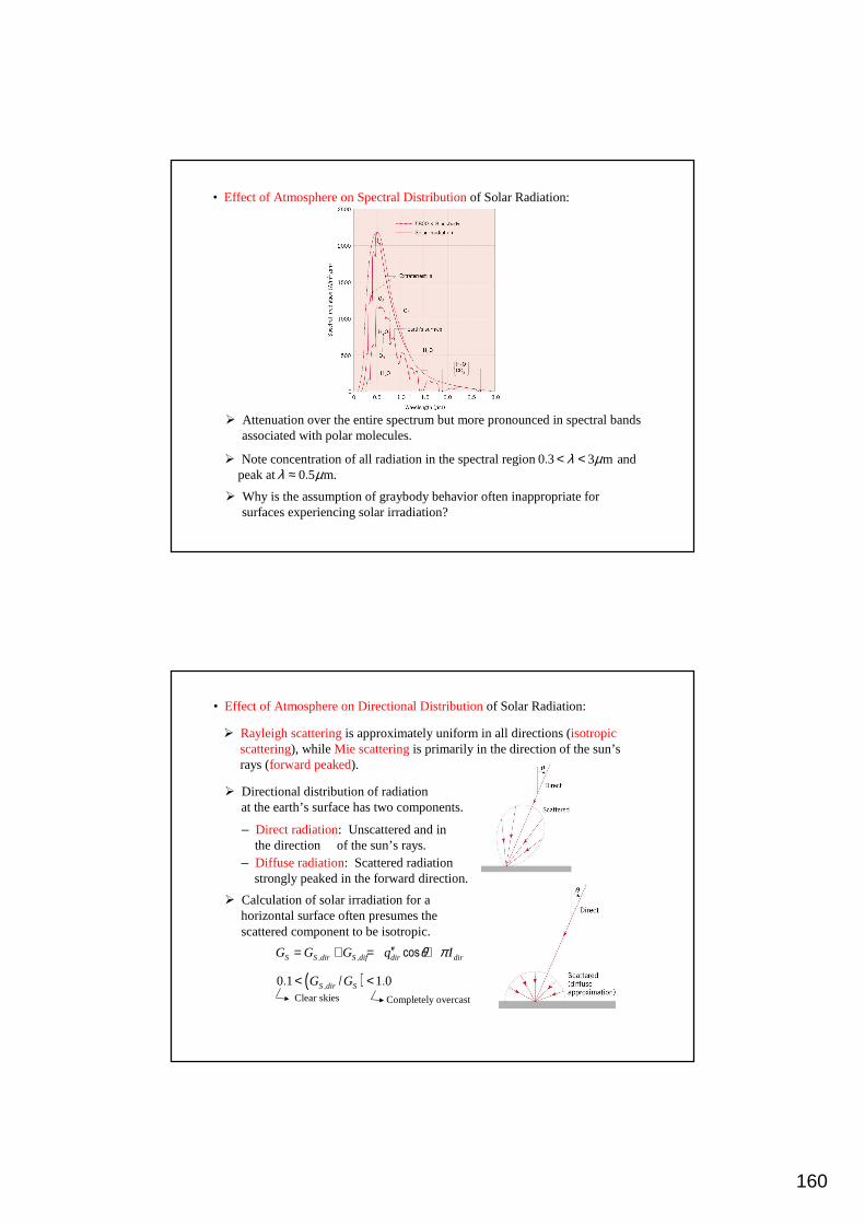
160

• Effect of Atmosphere on Spectral Distributionof Solar Radiation:

� Attenuation over the entire spectrum but more pronounced in spectral bandsassociated with polar molecules.

� Note concentration of all radiation in the spectral region andpeak at

0 3 3 m. λ µ< <0 5 m..λ µ≈

� Why is the assumption of graybody behavior often inappropriate forsurfaces experiencing solar irradiation?

• Effect of Atmosphere on Directional Distributionof Solar Radiation:

� Rayleigh scatteringis approximately uniform in all directions (isotropic scattering), while Mie scatteringis primarily in the direction of the sun’srays (forward peaked).

� Directional distribution of radiationat the earth’s surface has two components.

– Direct radiation: Unscattered and inthe direction of the sun’s rays.θ

– Diffuse radiation: Scattered radiationstrongly peaked in the forward direction.

� Calculation of solar irradiation for a horizontal surface often presumes thescattered component to be isotropic.

, ,cosS S dir S dif dir dirG G G q Iθ π′′= + = +

( )0 1 1 0,

. / .S dir SG G< <Clear skies Completely overcast

161

Terrestrial Radiation• Emission by Earth’s Surface:

4E Tεσ=

� Emissivities are typically large. For example, from Table A.11:

Sand/Soil: 0 90Water/Ice: 0 95Vegetation: 0 92Snow: 0 82Concrete/Asphalt: 0 85

.

.

.

.

.

εεεεε

>>>>>

� Emission is typically from surfaces with temperatures in the range of250 < T < 320K and hence concentrated in the spectral region

with peak emission at 4 40 m,λ µ< < 10 m.λ µ≈

• Atmospheric Emission:

� Largely due to emission from CO2 and H2O (v) and concentrated in the spectral regions 5 8 m and 13 m.λ µ λ µ< < >

� Although far from exhibiting the spectral characteristics of blackbody emission,earth irradiation due to atmospheric emissionis often approximated by ablackbody emissive power of the form

4atm skyG Tσ=

effective sky te mperatu et re hskyT →

230K< 285KskyT <Cold, clear sky Warm, overcast sky

• Can water in the natural environment freeze if the ambient air temperatureexceeds 273K? If so, what environmental conditions (wind and sky) favor ice formation?

162

Surface Radiative Properties• Concentration of solar and terrestrial in

different spectral regions often precludes use of the gray surface approximation.

( )0 3 3 m. λ µ< < ( )4 40 mλ µ< <

( )Sε α≠

� Note significant differences in for the two spectral regions: snow,human skin, white paint.

and λ λρ α

� In terms of net radiation transfer to a surface with solar irradiation, the parameterhas special significance. Why?/Sα ε

3.0Evaporated Al film

1.0Black paint

0.22White paint

0.64Human skin

0.29Snow

Surface /Sα ε

Rejection

Collection

163

Problem 12.119: Determination of preferred roof coating (Parsons Black, Acrylic White, or Zinc Oxide White) and corresponding heat load for prescribed operating conditions.

KNOWN: Dimensions and construction of truck roof. Roof interior surface temperature. Truck speed, ambient air temperature, and solar irradiation.

FIND: (a) Preferred roof coating, (b) Roof surface temperature, (c) Heat load through roof, (d) Effect of velocity on surface temperature and heat load.

ASSUMPTIONS: (1) Turbulent boundary layer development over entire roof, (2) Constant properties, (3) Negligible atmospheric (sky) irradiation, (4) Negligible contact resistance.

PROPERTIES: Table A.4, Air (Ts,o ≈ 300 K, 1 atm): 6 215 10 m sν −= × , k 0.026 W m K= ⋅ , Pr = 0.71.

ANALYSIS: (a) To minimize heat transfer through the roof, minimize solar absorption relative to surface emission. Hence, from Table A.12, use zinc oxide white for which αS = 0.16 and ε = 0.93.

(b) Performing an energy balance on the outer surface of the roof, S S conv condG q E q 0α ′′ ′′+ − − = ,

it follows that

4S S s,o s,o s,o s,iG h(T T ) T (k t)(T T )α εσ∞+ − = + −

SCHEMATIC:

164

where it is assumed that convection is from the air to the roof. With

7L 6 2

30 m s(5m)VLRe 10

15 10 m sν −= = =

×

4 / 5 1/ 3 7 4 / 5 1/ 3L LNu 0.037 Re Pr 0.037(10 ) (0.71) 13,141= = =

2Lh Nu (k L) 13,141(0.026 W m K/5m 68.3W m K= = ⋅ = ⋅ .

Substituting numerical values in the energy balance and solving by trial-and-error, we obtain Ts,o = 295.2 K.

(d) From parametric calculations based on the foregoing model, the following results are obtained.

(c) The heat load through the roof is

2s s,o s,iq (kA t)(T T ) (0.05 W m K 10 m 0.025m)35.2 K 704 W= − = ⋅ × = .

5 10 15 20 25 30

Velocity, V(m/s)

280

285

290

295

300

Tem

pera

ture

, Tso

(K)

5 10 15 20 25 30

Velocity, V(m/s)

500

550

600

650

700

Hea

t loa

d, q

(W)

The surface temperature and heat load decrease with decreasing V due to a reduction in the convection heat transfer coefficient and hence convection heat transfer from the air.

COMMENTS: The heat load would increase with increasing αS/ε.

165

Trocas radiativas entre superfícies: recintos fechados com meio não participativo

Conceitos básicos

• Recinto fechadoconsiste de 2 ou mais superfícies que englobam uma região do espaço (tipicamente preenchida com gás) e que trocam energia radiativa entre si.

• Um meio não participativo,num recinto fechado, não emite, não absorve,nem sofre scatteringde energia radiativa. Portanto, não produz qualquer efeito nastrocas de radiação entre as superfícies.

• Cada superfície que limita o recinto fechado é suposta ser isotérmica, opaca, difusae cinzenta, sendo caracterizada por radiosidadee irradiação uniformes.


i jij

i i

qF

A J→=

21 cos cos

i j

i jij i jA A

i

F dA dAA R

θ θπ

= ∫ ∫

2

cos coscos

i ji j i i i j i i i jdq I dAd J dAdA

R

θ θθ ω

π→ −= =

O Factor de Forma• O factor de forma, , é uma quantidade geométrica correspondente àfracção da radiação que abandona a superfície i e que é intersectada pela superfíciej.

,ijF

Considere a troca entre duas áreas diferenciais:

166


21 cos cos

ji

i jji i jAA

j

F dAdAA R

θ θπ

= ∫ ∫

i ij j jiA F A F=

Relações para o Factor de Forma

• Relação de Reciprocidade:

• Regra da Somatóriopara recintos fechados.

11

N

ijj

F=

=∑


Relações para o Factor de Forma

• Geometrias Bi-Dimensionais(Tabela 13.1). Por exemplo,

Um Plano Infinito e uma Fileira de Cilindros

( ) ( )1 2 1 22 2 2

121 1

/ /

tanijD D s DFs s D

− −= − − +

167


( )1 222

2

2

1 42

11

/

/

/ /

ij j i

j

i

i i j j

F S S r r

RS

R

R r L R r L

= − −

+= +

= =

Relações para o Factor de Forma• Geometrias Tri-Dimensionais(Tabela 13.2). Por exemplo,

Discos Coaxiais Paralelos


FACTORES DE FORMA – MÉTODO DAS CORDAS

PERMITE CALCULAR ÁREAS DE PERMUTA, AiFij, ENTRE 2 SUPERFÍCIES i E j QUE OBEDECEM ÀS SEGUINTES CONDIÇÕES:

• COMPRIMENTO MUITO MAIOR QUE A DISTÂNCIA QUE AS SEPARA• SECÇÕES RECTAS CONSTANTES E PERPENDICULARES AO COMPRIMENTO• DISTÂNCIA QUE AS SEPARA SER CONSTANTE

A1

A2

168


L3

L4

L2

L1

FACTORES DE FORMA – MÉTODO DAS CORDAS

( ) ( )2

2

2121121

121

LLLLFA

cruzadasnãocordascruzadascordasFA

+−+=

−= ∑∑

21 cos cos

i j

i jij i jA A

i

F dAdAA R

θ θπ

= ∫ ∫

2

cos coscos

i ji j i i i j i i i jdq I dAd J dAdA

R

θ θθ ω

π→ −= =


FACTORES DE FORMA ENTRE RECTÂNGULOS DIAMETRALMENTE OPOSTOS

APLICA-SE QUANDO HÁ SIMETRIA OU SEMELHANÇA NA GEOMETRIA

343121 FAFA =

A1

A3

A2

A4

R

R

169


FACTORES DE FORMA – OUTRAS RELAÇÕES

( ) ∑=

=n

kikji FF

1

( ) ( )

( )( )j

n

kkik

ij

n

kkikijj

A

FAF

FAFA

∑

∑

=

=

=

=

1

1

Trocas radiativas entre superfícies negras

• Para um corpo negro, .i biJ E=

taxaútil à qual a radiaçãoabandona a superfíciei devidoà sua interacção com j

ou taxaútil à qual a superfíciejganha radiação devido àsua interacção com i

Transferência de radiação útil da superfíciei devido a trocas com todas as (N) superfícies num recinto fechado:

• Troca de calor útil entre duas superfíciesque podem ser aproximadas como corposnegros

ij i j j iq q q→ →= −

ij i ij bi j ji bjq A F E A F E= −

( )4 4ij i ij i jq A F T Tσ= −

( )4 4

1

N

i i ij i jj

q A F T Tσ=

= −∑

170

Troca radiativa entre as N superfícies opacas, difusas e cinzentas de um recinto fechado

• Expressões alternativas paratransferência radiativaútil a partir da superfíciei:

Sugere umaresistencia da superfícieradiativa da forma: ( )1 /i i iAε ε−

( ) Fig. (b)i i i iq A J G= − → (1)( ) Fig. (b)i i i iq A J G= − → (1)

( ) Fig. (c)i i i i iq A E Gα= − → (2)( ) Fig. (c)i i i i iq A E Gα= − → (2)

( ) Fig. (d)

1 /

bi ii

i i i

E Jq

Aε ε−= →

−(3)

( ) Fig. (d)

1 /

bi ii

i i i

E Jq

Aε ε−= →

−(3)

Troca radiativa entre as N superfícies opacas, difusas e cinzentas de um recinto fechado

( )( ) 1

1 1

N N i ji i ij i j

j ji ij

J Jq A F J J

A F−

= =

−= − =∑ ∑ (4)( )

( ) 11 1

N N i ji i ij i j

j ji ij

J Jq A F J J

A F−

= =

−= − =∑ ∑ (4)

( ) ( ) 111 /

Ni jbi i

ji i i i ij

J JE J

A A Fε ε −=

−− = ∑−

(5)( ) ( ) 1

11 /

Ni jbi i

ji i i i ij

J JE J

A A Fε ε −=

−− = ∑−

(5)

Sugere umaresistência espacialou geométricada forma: ( ) 1

i ijA F−

• Igualando as Eqs. (3) e (4) corresponde a um balançode energia radiativaà superfíciei:

que pode ser representadopor um análogo eléctricodo tipo:

171

Metodologia de análise para recintos fechados

� Aplicar Eq. (4) a cada superfície para a qual o fluxo útil de radiaçãoé connecido.

iq

� Aplicar Eq. (5) a cada uma das restantes superfícies paraa qual a temperatura , e, portanto, , é conhecida.

iT,biE

� Calcular todos os factores de forma que aparecem nas equações

� Resolver o sistema de N equações para as radiosidades (incógnitas)1 2, ,...., .NJ J J

• Tratamento de superfície virtual correspondente a aberturade área , através daas superfícies interiores de um recinto fechado trocam radiação com a envolvente(de grandes dimensões) à temperatura :

iA

surT

� Aproximar a abertura a um corpo negro de área, temperatura, e propriedades, .

,iA ,i surT T=1i iε α= =

� Usar Eq. (3) para determinarqi para cada superfície onde se conheceTi e para determinarTi para cada superfície onde se conheceqi.

Recintos fechados com duas superfícies

( )4 41 2

1 2 121 2

1 1 1 12 2 2

1 11

T Tq q q

A A F A

σε ε

ε ε

−= − = = − −+ +

Recinto mais simples para o qual a troca de calor por radiação se dáexclusivamente entre duas superfícies e em que uma expressão para a troca de calor por radiação pode ser determinada directamente através do análogo eléctrico.

172

• A tabela 13.3 apresenta resultados para alguns casos especiais. Por exemplo:

� Placas paralelas e infinitas

1 2

12 1

A A A

F

= ≡

=

( )4 41 1 2

12

1 2

1 1 1

A T Tq

σ

ε ε

−=

+ −

� Pequena superfície plana/convexa rodeada por uma superfície muito maior

1

0

, =

=

surs

sur

s

F

A

A

( )44sursss TTAq −= σε

Escudo de radiação

• Superfície com reflectividade elevada (baixoα = ε) colocada entre duassuperfícies cuja troca de calor por radiação se pretende reduzir

α ε=

• Considere um único escudo de radiação num reconto fechado, tal como é o caso de duas placas planas paralelas e infinitas.

Note que, embora raramente, a emissão pode ser diferente para as duas superfícies do

escudo de radiação.

173

Análogo eléctrico

( )4 41 2

12 1 23 1 3 21 2

1 1 1 13 3 1 3 3 2 3 3 32 2 2

1 11 11 1, ,

, ,

T Tq q q

A A F A A A F A

σε εε ε

ε ε ε ε

−= = − = − −− −+ + + + +

• O resultado anterior pode ser facimente estendido parater em conta múlitplos

escudos de radiação e aplicado a cilindros longos e concêntricos, esferas

concêntricas e placas longas e paralelas.

A superficie re-radiante

( )

( ) ( )

4 41 2

1 21 2

11 1 2 21 12 1 1 2 2

1 111 1/ /R R

T Tq q

A AA F A F A F

σε ε

ε ε−

−= − = − −+ +

+ +

• Uma idealização para a qual: .R RG J=

• Corresponde a superfícies que sãobem isoladas de um ladoe para as quaisa convecção é desprezável do lado oposto (radiante).

• Recinto fechado com três superfícies sendo uma delas re-radiante :

Portanto, and 0 .R R bRq J E= =

174

A superficie re-radiante

( ) ( )1 2

1 1 2 21 1/ /

R R

R R

J J J J

A F A F

− −=

• Temperatura da superfícre re-radiante pode ser determinada a partir do conhecimentoda sua radiosidade .

RT

RJ

1 4/

RR

JT

σ =

Problem 13.88: Power requirement for a cylindrical furnace with tworeradiating surfaces and an opening to large surroundings.

KNOWN: Cylindrical furnace of diameter D = 90 mm and overall length L = 180 mm. Heating elements maintain the refractory lining (ε = 0.8) of section (1), L1 = 135 mm, at T1 = 800°C. The bottom (2) and upper (3) sections are refractory lined, but are insulated. Furnace operates in a spacecraft vacuum environment.

FIND: Power required to maintain the furnace operating conditions with the surroundings at 23°C.

175

SCHEMATIC:

ASSUMPTIONS: (1) All surfaces are diffuse gray, and (2) Uniform radiosity over the sections 1, 2, and 3.

ANALYSIS: By defining the furnace opening as the hypothetical area A4, the furnace can be represented as a four-surface enclosure.

The power required to maintain A1 at T1 is q1, the net radiation leaving A1.

To obtain q1, we must determine the radiosity at each surface by simultaneously solving radiation energy balance equations of the form

( )

Nj jbi i

ii i i i ijj 1

J JE Jq

1 / A 1/ A Fε ε =

−−= =

− ∑ (1,2)

However, since ε4 = 1, J4 = Eb4, and only three energy balances are needed for A1, A2, and A3.

A1: ( )b1 1 1 31 2 1 4

1 1 1 1 12 1 13 1 14

E J J JJ J J J

1 / A 1/ A F 1/ A F 1/ A Fε ε− −− −

= + +−

(3)

A2: 2 32 1 2 4

2 21 2 23 2 24

J JJ J J J0

1/ A F 1/ A F 1/ A F

−− −= + + (4)

A3: 3 1 3 2 3 4

3 31 3 32 3 34

J J J J J J0

1/ A F 1/ A F 1/ A F

− − −= + + (5)

where q2 = q3 = 0 since the surfaces are insulated (adiabatic) and hence reradiating.

From knowledge of J1, q1 can be determined using Eq. (1).

Of the N2 = 42 = 16 view factors, N(N – 1)/2 = 6 must be independently evaluated, while the remaining can be determined by the summation rule and appropriate reciprocity relations. The six independently determined Fij are:

By inspection: (1) F22 = 0 (2) F44 = 0

176

Coaxial parallel disks: From Table 13.2,

(3) ( )1/ 222

24 4 2F 0.5 S S 4 r / r 0.05573= − − =

where 2 24

2 2 4 42 22

1 R 1 0.250S 1 1 18.00 R r / L 45 /180 0.250 R r / L 0.250

R 0.250

+ += + = + = = = = = =

Enclosure 1-2-2′: From the summation rule for A2, (4) F21 = 1 – F22′ = 1 – 0.09167 = 0.9083 where F22′ can be evaluated from the coaxial parallel disk relation, Table 13.2, with R2 = r2/L1 = 45/135 = 0.333, R2′ = r2/L1 = 0.333, and S = 11.00.

From the summation rule for A1,

(5) F11 = 1 – F12 – F12′ = 1 – 0.1514 – 0.1514 = 0.6972

From symmetry F12 = F12′ and using reciprocity

( )( )[ ]12 2 21 1F A F / A 0.090m 2 / 4 0.9083 / 0.090m 0.135m 0.1514π π= = × × × =

Enclosure 2′ -3-4: From the summation rule for A4,

(6) F43 = 1 – F42′ – F44 = 1 – 0.3820 – 0 = 0.6180

where F44 = 0 and using the coaxial parallel disk relation from Table 13.2, F42′ =0.3820 with R4 =

r4/L2 = 45/45 = 1, R2′ = r2/L2 = 1, and S = 3.

From knowledge of the relevant view factors, the energy balances, Eqs. (3, 4, 5), can be solved simultaneously to obtain the radiosities,

2 2 21 2 3J 73,084 W / m J 67,723W / m J 36,609 W / m= = =

The net heat rate leaving A1 can be evaluated using Eq. (1) written as

( )

( )( )

2b1 1

1 21 1 1

75,159 73,084 W / mE Jq 317 W

1 / A 1 0.8 / 0.8 0.03817 mε ε−−

= = =− − ×

<

where Eb1 = 41Tσ = σ(800 + 273K)4 = 75,159 W/m2 and A1 = πDL1 = π × 0.090m × 0.135m =

0.03817 m2.

COMMENTS: Recognize the importance of defining the furnace opening as the hypothetical area A4 which completes the four-surface enclosure representing the furnace. The temperature of A4 is that of the surroundings and its emissivity is unity since it absorbs all radiation incident on it.

The View Factors: Using summation rules and appropriate reciprocity relations, the remaining 10 view

factors can be evaluated. Written in matrix form, the Fij are 0.6972* 0.1514 0.09704 0.05438 0.9083* 0* 0.03597 0.05573* 0.2911 0.01798 0.3819 0.3090 0.3262 0.05573 0.6180* 0*

The Fij shown with an asterisk were independently determined.

177

Problem 13.93: Assessment of ceiling radiative properties for an ice rinkin terms of ability to maintain surface temperature above the dewpoint.

KNOWN: Ice rink with prescribed ice, rink air, wall, ceiling and outdoor air conditions.

FIND: (a) Temperature of the ceiling, Tc, for an emissivity of 0.05 (highly reflective panels) or 0.94 (painted panels); determine whether condensation will occur for either or both ceiling panel types if the relative humidity of the rink air is 70%, and (b) Calculate and plot the ceiling temperature as a function of ceiling insulation thickness for 0.1 ≤ t ≤ 1 m; identify conditions for which condensation will occur on the ceiling.

SCHEMATIC:

ASSUMPTIONS: (1) Rink comprised of the ice, walls and ceiling approximates a three-surface, diffuse-gray enclosure, (2) Surfaces have uniform radiosities, (3) Ice surface and walls are black, (4) Panels are diffuse-gray, and (5) Thermal resistance for convection on the outdoor side of the ceiling is negligible compared to the conduction resistance of the ceiling insulation.

178

PROPERTIES: Psychometric chart (Atmospheric pressure; dry bulb temperature, Tdb = T∞,i = 15°C; relative humidity, RH = 70%): Dew point temperature, Tdp = 9.4°C.

ANALYSIS: Applying an energy balance to the inner surface of the ceiling and treating all heat rates as energy outflows, in outE E 0− =& &

o conv,c rad,cq q q 0− − − = (1)

From Table 13.2 for parallel, coaxial disks icF 0 672.=

From the summation rule applied to the ice (i) and the reciprocity rule, ic iw iw cwF F 1 F F (symmetry)+ = =

cw icF 1 F= −

( ) ( ) ( )wc c w cw c w icF A A F A A 1 F 0 410/ / .= = − =

where Ac = π D2/4 and Aw = π DL.

where the rate equations for each process are

( )o c ,o cond cond cq T T / R R t / kA∞= − = (2,3)

( )conv,c i c c ,iq h A T T∞= − (4)

Since the ceiling panels are diffuse-gray, α = ε.

( ) ( ) ( )rad,c b c c w wc b w i ic b iq E T A A F E T A F E Tε α α= − − (5)

(b) Applying the foregoing model for 0 1 1 0 m. . ,t≤ ≤ the following result is obtained

0 0.2 0.4 0.6 0.8 1

Ceiling insulation thickness, t (m)

5

10

15

Cei

ling

tem

pera

ture

, Tc

(C)

Painted ceiling, epsc = 0.94Reflective panel, epsc = 0.05

Using the foregoing energy balance, Eq. (1), and the rate equations, Eqs. (2-5), the ceiling temperature is calculated using radiative properties for the two panel types, Ceiling panel ε Tc (°C) Reflective 0.05 14.0 Paint 0.94 8.6 Tc < Tdp <

. Condensation will occur on the painted panel since Tc < Tdp.

b) Applying the foregoing model for 0.1 ≤ t ≤ 1.0 m the following result is obtained

179

For the reflective panel (ε = 0.05), the ceiling surface temperature is considerably above the dew point. Therefore, condensation will not occur for the range of insulation thicknesses. For the painted panel (ε = 0.94), the ceiling surface temperature is always below the dew point, and condensation occurs for the range of insulation thicknesses.

COMMENTS: From the analysis, recognize that radiative exchange between the ice and the ceiling has the dominant effect on the ceiling temperature. With the reflective panel, the rate is reduced nearly 20-fold relative to that for the painted panel. With the painted panel ceiling, condensation will occur for most of the conditions likely to exist in the rink.

slides transmissão de calor

Documents