slawomir koziel, qingsha s. cheng, and john w. bandler ieomc.ru.is/eoml_pdf/paper_1.pdf · digital...

Digital Object Identifier 10.1109/MMM.2008.929554

©DIGITAL VISION

Slawomir Koziel, Qingsha S. Cheng, and John W. Bandler

In this article we review state-of-the-art con-cepts of space mapping and place them con-textually into the history of design optimiza-tion and modeling of microwave circuits. Weformulate a generic space-mapping optimiza-

tion algorithm, explain it step-by-step using a sim-ple microstrip filter example, and then demonstrateits robustness through the fast design of an interdig-ital filter. Selected topics of space mapping are dis-cussed, including implicit space mapping, gradient-based space mapping, the optimal choice of surro-gate model, and tuning space mapping. We consid-er the application of space mapping to the modelingof microwave structures. We also discuss a softwarepackage for automated space-mapping optimizationthat involves both electromagnetic (EM) and circuitsimulators.

A Brief History of Microwave CAD

Early DevelopmentsIn 1967, in a benchmark paper [1], Temes andCalahan presented an extensive and detailed reviewof general-purpose optimization algorithms usefulfor computer-aided network design. They providedstate-of-the-art examples of network optimizationthrough specialized iterative techniques. Theirpaper was the first comprehensive review of itskind. In ensuing years, Bandler [2], [3] systematical-ly treated the formulation of error functions withregard to design specifications. He explored least pthand minimax objectives, nonlinear constraints, gra-dient and direct search methods, as well as adjoint

Slawomir Koziel is with the School of Science and Engineering, Reykjavik University, Kringlunni 1,

IS-103 Reykjavik, Iceland. Qingsha S. Cheng and John W. Bandler are with the

Simulation Optimization Systems Research Laboratory,Department of Electrical and Computer Engineering,

McMaster University, Hamilton, ON, Canada L8S 4K1. John W. Bandler is also with Bandler Corporation,

Dundas, ON L9H 5E7, Canada.

December 2008 1051527-3342/08/$25.00©2008 IEEE

Authorized licensed use limited to: Reykjavik University. Downloaded on November 20, 2008 at 00:49 from IEEE Xplore. Restrictions apply.

106 December 2008

circuit sensitivity analysis techniques suitable formicrowave circuit simulation and design.

The complexity of microwave devices has continuedto increase, especially after the emergence and produc-tion of monolithic microwave integrated circuits(MMICs) [4] in the 1970s. Bandler et al. [5] demonstrat-ed the automated optimization of a large-scale designof a 12-GHz multiplexer with 16 channels and 240 non-linear design variables. In a 1988 review paper, Bandlerand Chen [6] emphasized optimization-orientedapproaches to deal more explicitly with process impre-cision, manufacturing tolerances, model uncertainties,measurement errors, and so on, approaches well suitedto yield enhancement and cost reduction for integratedcircuits. Bandler and Salama [7] addressed circuit tun-ing for postproduction alignment.

Credit for the first commercial microwave circuitoptimization software should be given to Les Besser forhis COMPACT (Computer Optimization of MicrowavePassive and Active CircuiTs) in 1973. Its successor,SuperCOMPACT, became an industry standard [8].EEsof (now Agilent Technologies) launched its circuitsimulator TOUCHSTONE in 1983. In 1985, Bandlerintroduced powerful minimax optimizers into EEsof’sTOUCHSTONE. TOUCHSTONE evolved into Libraafter harmonic balance simulation was added [8].

Techniques for design centering, tolerance assign-ment, worst-case and statistical design, and postpro-duction tuning evolved during the 1970s [9], peakingin the late 1980s when Optimization SystemsAssociates (OSA) introduced yield-driven design intoSuperCOMPACT. EEsof followed suit with yield-dri-ven design options. The 1980s also saw advances androbust implementation in software of gradient-basedalgorithms for minimax, l1, and l2 optimization [6].

Meanwhile, during the 1980s, Ansoft Corporation,Hewlett-Packard, and Sonnet Software embarked on thedevelopment of simulators that solved Maxwell’s equa-tions for complex geometries. Denoted EM simulators orsolvers, they were originally applied to obtain accurate sim-ulations or validations of complex microwave structures.

EM-Based OptimizationThe idea of employing EM solvers for direct optimaldesign attracted microwave engineers. However, EMsolvers are notoriously CPU-intensive. As originally con-strued, they also suffered from nondifferentiableresponse evaluation and nonparameterized design vari-ables that were discrete in the parameter space. Suchcharacteristics are unfriendly to available efficient gradi-ent optimization algorithms. To alleviate this, Bandler etal. proposed some breakthrough techniques, such as theutilization of databases [10]–[12], the Datapipe concept[10], multidimensional interpolation [11]–[13], geometrycapture [11], [12], [14] for parameterization, and the prag-matic idea of the simulation grid. Formal EM optimiza-tion of planar and three-dimensional (3-D) microwavestructures has been reported since 1994 [15]–[18].

In 1990, through Optimization Systems Associates,Bandler introduced OSA90, the world’s first friendlymicrowave optimization engine for performance-dri-ven and yield-driven design. It incorporated state-of-the-art microwave circuit simulation and optimizationalgorithms. It provided an interface to external simula-tors, circuit based or EM based. In Swanson’s words,“[OSA90 is] the first commercially successful optimiza-tion scheme which included a field-solver inside theoptimization loop” [19], [20]. The success of OSA’s tech-nology and software prompted HP (now AgilentTechnologies) to acquire OSA [21].

Our goal is to find a fine model optimal solution

x∗ = arg minx

U(Rf (x)). (1)

Here, the fine-model response vector is denoted by Rf ,e.g., |S21| at selected frequency points. The fine-modeldesign parameters are denoted x. U is a suitable objectivefunction. In microwave engineering, U is typically a mini-max objective function with upper and lower specifications[2], [3], [6]; x∗ is the optimal design to be determined.

Generic space mapping uses the following iterativeprocedure to solve (1):

xk+1 = arg minx

U(Rs(x, pk)) (2)

where Rs(x, p) is a response vector of the space-mapping surrogate model with x and p as the design

variables and model parameters, respectively. Inimplicit space mapping [31], the model parametersare the so-called preassigned parameters. Parameterspk are obtained at iteration k using the parameterextraction procedure

pk = arg minp

k∑

j=0

wj‖Rf (xk) − Rs(xk, p)‖ (3)

in which we try to match the surrogate to the finemodel. wj are weighting factors that determine thecontribution of previous iteration points to the para-meter extraction process [39]. The surrogate modelis normally the coarse model Rc composed withsuitable transformations; e.g., the input space-map-ping surrogate is defined as a linear distortion ofthe coarse model domain:Rs(x, p) = Rs(x, B, c) = Rc(B · x + c) .

The Space-Mapping Optimization Algorithm


December 2008 107

Nevertheless, the successful interconnection of EMsolvers with powerful optimization techniques onlypartially solved the EM-based design bottleneck, sinceEM simulation remained CPU-intensive. Thus, conven-tional mathematical optimization algorithms insuffi-ciently satisfied the microwave community’s ambitionsfor automated EM-based design optimization. In the1990s, EM modeling and optimization were exploredthrough novel technologies such as response surfacemodeling [13], model-reduction techniques [22], andartificial neural networks [23].

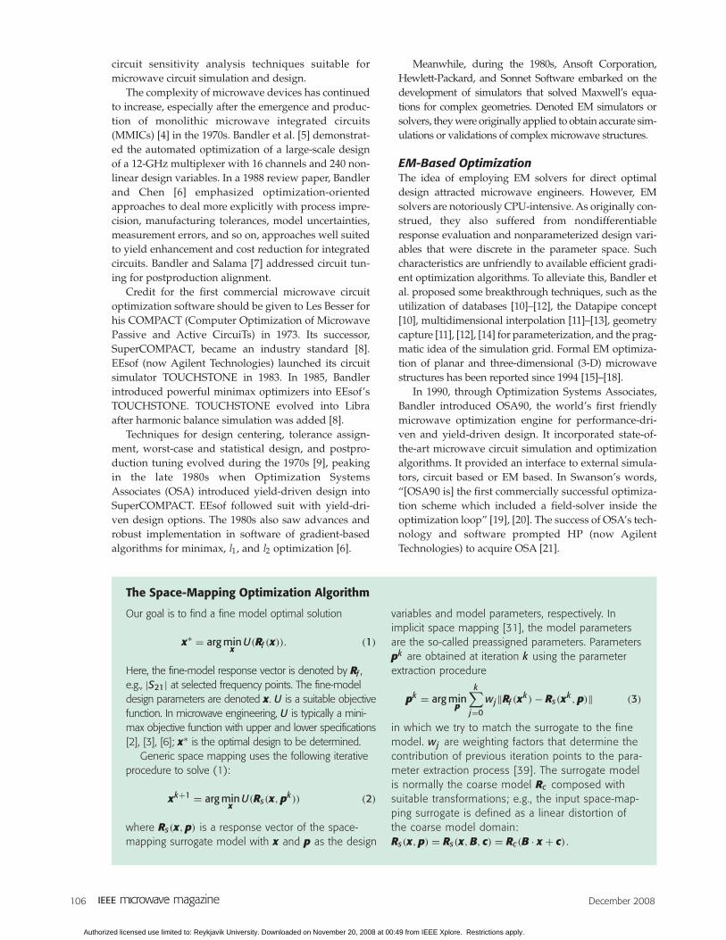
Space MappingIn 1994, Bandler et al. [24] proposed a simple but effec-tive idea to automatically mate the efficiency of circuitoptimization with the accuracy of EM solvers. The ideawas to map designs from optimized circuit models tocorresponding EM models. Clearly, discrepancies wereexpected. A “parameter extraction” step calibrated thecircuit solver against the EM simulator so that observeddifferences between the EM and circuit simulationswere minimized. The circuit model (surrogate) wasthen updated with extracted parameters and madeready for subsequent efficient optimization.

This methodology is named space mapping. It uti-lizes a “coarse” model (analytical approximation ofthe physics of the device under investigation) toobtain a near optimal design of an accurate EM-based“fine” model. The coarse model may be a circuit sim-ulator such as Agilent ADS [25]. The fine model is nor-mally an EM simulator based on the method ofmoments (MoM) (e.g., Agilent Momentum [26] andSonnet em [27]), finite element (e.g., Ansoft HFSS [28]),FDTD (e.g., FEKO [29]), or TLM (e.g., MEFiSTo [30]).See Figure 1. A link or mapping between the fine andthe coarse models is established and updated througha parameter extraction process. The mapped coarsemodel or updated surrogate may be re-optimized toobtain a new design.

Space-mapping optimization belongs to the class ofsurrogate-based optimization methods [32], which gener-ate a sequence of approxima-tions to the objective functionand manage the use of theseapproximations as surrogatesfor optimization. In microwaveand RF engineering, surrogatesthat can be efficiently opti-mized include lumped or dis-tributed element equivalentcircuit models (companionmodel [33]), EM scatteringmatrix models with tuningports [34], [35], circuit modelswith embedded EM compo-nents [36], or interpolatedcoarse-grid EM models [37].

Surrogate-based optimization has become an EMoptimization approach of choice: in [38] Rautio said,“Today, I find that most designers use either a tuningmethodology, a companion modeling methodology, orsome combination of the two to tune the final designwith EM analysis.”

In this ArticleWe organize our article as follows. In the next section,we recall the concept of space mapping and formulatethe space-mapping optimization algorithm. We alsoexplain and illustrate the space-mapping optimizationprocess using a simple bandstop microstrip filter exam-ple. Then, we demonstrate the robustness of this tech-nology through an accurate design of an interdigital fil-ter. The subsequent sections contain an exposition ofselected topics and recent developments in space-map-ping technology, including implicit and output spacemapping, gradient-based space mapping, as well astuning space mapping. We also discuss the issue of anoptimal choice of surrogate model to be used in space-mapping optimization, the implementation of spacemapping in device modeling, as well as the SpaceMapping Framework (SMF)—a user-friendly space-mapping software system.

Space Mapping Optimization

Space-Mapping Optimization ConceptThe formulation of the space mapping optimizationalgorithm [39] is presented in “The Space-MappingOptimization Algorithm” [31], [39]. Our goal is toobtain the fine model optimal design without directoptimization of the fine model. Instead, we want touse the surrogate model; i.e., the coarse model com-posed with suitable auxiliary mappings. The values ofthe relevant parameters of these mappings are updat-ed during each iteration of the algorithm using a so-called parameter extraction procedure in order toobtain as good a match between the surrogate modeland the fine model as possible. The surrogate model is

Figure 1. Space-mapping implementation concept [31].

FineSpace

CoarseSpace

Obtain a Mapping to Match the Models(Parameter Extraction)

(Surrogate Optimization)Obtain New Prediction

Fine ModelCoarse Model

AgilentADS

MomentumSonnet em

Ansoft HFSS

DesignParameters

ResponsesDesignParameters

Responses

PreassignedParameters

Agilent ADS


108 December 2008

then optimized and its optimal solution is consideredto be a new design. Parameter extraction and designupdating are performed solely on the surrogate modelso that both require little computational overheadsince the coarse model is assumed to be substantiallycheaper than the fine model. The fine model is onlyevaluated at the new design for verification purposesand also to provide data for the next iteration of thealgorithm. Typically, fine model sensitivity is notinvolved in the process.

A crucial prerequisite is that the coarse model isphysically based; i.e., it describes the same physicalphenomena as the fine model, however, with less accu-racy. Due to this, the space-mapping surrogate hasexcellent generalization properties even if it is estab-lished using a small amount of fine model data, and thespace-mapping optimization process yields satisfactoryresults after only few evaluations of the fine model.

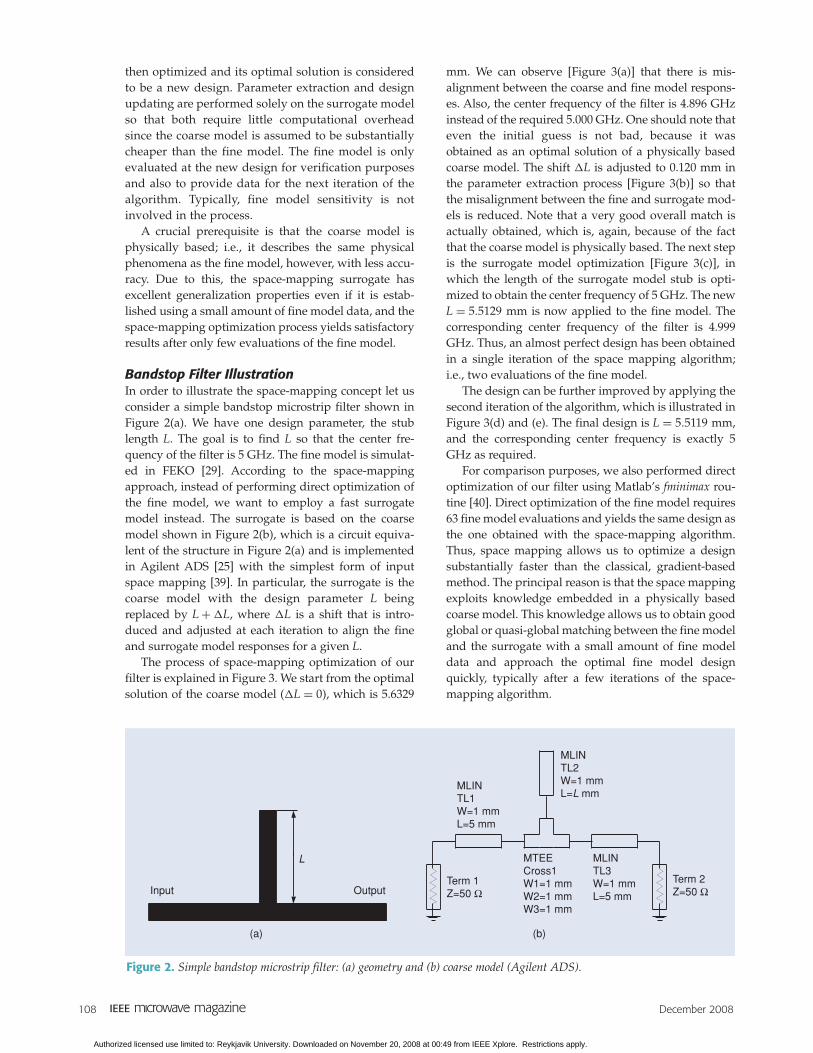
Bandstop Filter IllustrationIn order to illustrate the space-mapping concept let usconsider a simple bandstop microstrip filter shown inFigure 2(a). We have one design parameter, the stublength L. The goal is to find L so that the center fre-quency of the filter is 5 GHz. The fine model is simulat-ed in FEKO [29]. According to the space-mappingapproach, instead of performing direct optimization ofthe fine model, we want to employ a fast surrogatemodel instead. The surrogate is based on the coarsemodel shown in Figure 2(b), which is a circuit equiva-lent of the structure in Figure 2(a) and is implementedin Agilent ADS [25] with the simplest form of inputspace mapping [39]. In particular, the surrogate is thecoarse model with the design parameter L beingreplaced by L + �L, where �L is a shift that is intro-duced and adjusted at each iteration to align the fineand surrogate model responses for a given L.

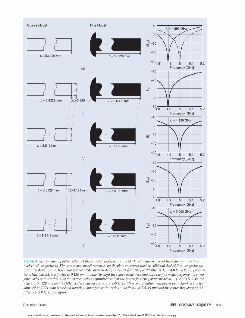
The process of space-mapping optimization of ourfilter is explained in Figure 3. We start from the optimalsolution of the coarse model (�L = 0), which is 5.6329

mm. We can observe [Figure 3(a)] that there is mis-alignment between the coarse and fine model respons-es. Also, the center frequency of the filter is 4.896 GHzinstead of the required 5.000 GHz. One should note thateven the initial guess is not bad, because it wasobtained as an optimal solution of a physically basedcoarse model. The shift �L is adjusted to 0.120 mm inthe parameter extraction process [Figure 3(b)] so thatthe misalignment between the fine and surrogate mod-els is reduced. Note that a very good overall match isactually obtained, which is, again, because of the factthat the coarse model is physically based. The next stepis the surrogate model optimization [Figure 3(c)], inwhich the length of the surrogate model stub is opti-mized to obtain the center frequency of 5 GHz. The newL = 5.5129 mm is now applied to the fine model. Thecorresponding center frequency of the filter is 4.999GHz. Thus, an almost perfect design has been obtainedin a single iteration of the space mapping algorithm;i.e., two evaluations of the fine model.

The design can be further improved by applying thesecond iteration of the algorithm, which is illustrated inFigure 3(d) and (e). The final design is L = 5.5119 mm,and the corresponding center frequency is exactly 5GHz as required.

For comparison purposes, we also performed directoptimization of our filter using Matlab’s fminimax rou-tine [40]. Direct optimization of the fine model requires63 fine model evaluations and yields the same design asthe one obtained with the space-mapping algorithm.Thus, space mapping allows us to optimize a designsubstantially faster than the classical, gradient-basedmethod. The principal reason is that the space mappingexploits knowledge embedded in a physically basedcoarse model. This knowledge allows us to obtain goodglobal or quasi-global matching between the fine modeland the surrogate with a small amount of fine modeldata and approach the optimal fine model designquickly, typically after a few iterations of the space-mapping algorithm.

Figure 2. Simple bandstop microstrip filter: (a) geometry and (b) coarse model (Agilent ADS).

L

Input OutputTerm 1Z=50 Ω

Term 2Z=50 Ω

MLINTL1W=1 mmL=5 mm

MTEECross1W1=1 mmW2=1 mmW3=1 mm

MLINTL3W=1 mmL=5 mm

MLINTL2W=1 mmL=L mm

(a) (b)


December 2008 109

Figure 3. Space-mapping optimization of the bandstop filter; white and black rectangles represent the coarse and the finemodel stub, respectively. Fine and coarse model responses on the plots are represented by solid and dashed lines, respectively:(a) initial design L = 5.6329 mm (coarse model optimal design), center frequency of the filter is f0 = 4.896 GHz; (b) parame-ter extraction: �L is adjusted to 0.120 mm in order to align the coarse model response with the fine model response; (c) surro-gate model optimization: L of the coarse model is optimized so that the center frequency of the model at L + �L is 5 GHz; thenew L is 5.5129 mm and the filter center frequency is now 4.999 GHz; (d) second iteration (parameter extraction): �L is re-adjusted to 0.121 mm; (e) second iteration (surrogate optimization): the final L is 5.5119 mm and the center frequency of thefilter is 5.000 GHz, as required.

ΔL=0.120 mm

... ...

...

L = 5.6329 mmL = 5.6329 mm

L = 5.5129 mm

...

L = 5.5129 mm

Coarse Model Fine Model

... ...

L = 5.6329 mmL = 5.6329 mm

ΔL=0.121 mm

... ...

...

L = 5.5129 mmL = 5.5129 mm

L = 5.5119 mm

...

L = 5.5119 mm

(a)

(b)

(c)

(d)

(e)

4.8 4.9 5 5.1 5.2–50

–40

–30

–20

–10

–50

–40

–30

–20

–10Frequency [GHz]

4.8 4.9 5 5.1 5.2Frequency [GHz]

–50

–40

–30

–20

–10

4.8 4.9 5 5.1 5.2Frequency [GHz]

–50

–40

–30

–20

–10

4.8 4.9 5 5.1 5.2Frequency [GHz]

–50

–40

–30

–20

–10

4.8 4.9 5 5.1 5.2Frequency [GHz]

f0 = 4.999 GHz

f0 = 4.896 GHz

f0 = 5.000 GHz

|S21

||S

21|

|S21

||S

21|

|S21

|


110 December 2008

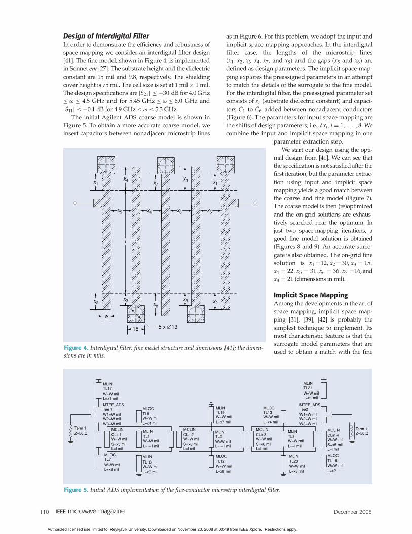
Design of Interdigital FilterIn order to demonstrate the efficiency and robustness ofspace mapping we consider an interdigital filter design[41]. The fine model, shown in Figure 4, is implementedin Sonnet em [27]. The substrate height and the dielectricconstant are 15 mil and 9.8, respectively. The shieldingcover height is 75 mil. The cell size is set at 1 mil × 1 mil.The design specifications are |S21| ≤ −30 dB for 4.0 GHz≤ ω ≤ 4.5 GHz and for 5.45 GHz ≤ ω ≤ 6.0 GHz and|S11| ≤ −0.1 dB for 4.9 GHz ≤ ω ≤ 5.3 GHz.

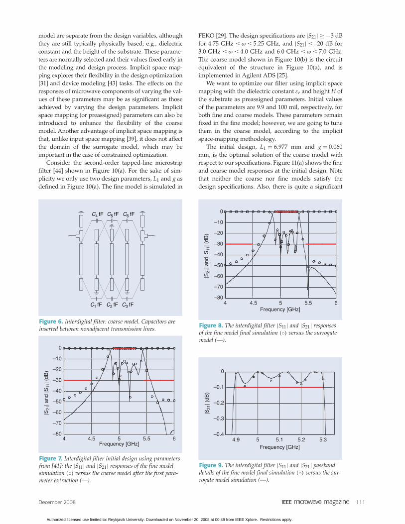
The initial Agilent ADS coarse model is shown inFigure 5. To obtain a more accurate coarse model, weinsert capacitors between nonadjacent microstrip lines

as in Figure 6. For this problem, we adopt the input andimplicit space mapping approaches. In the interdigitalfilter case, the lengths of the microstrip lines(x1, x2, x3, x4, x7, and x8) and the gaps (x5 and x6) aredefined as design parameters. The implicit space-map-ping explores the preassigned parameters in an attemptto match the details of the surrogate to the fine model.For the interdigital filter, the preassigned parameter setconsists of εr (substrate dielectric constant) and capaci-tors C1 to C6 added between nonadjacent conductors(Figure 6). The parameters for input space mapping arethe shifts of design parameters; i.e., δxi, i = 1, . . . , 8. Wecombine the input and implicit space mapping in one

parameter extraction step.We start our design using the opti-

mal design from [41]. We can see thatthe specification is not satisfied after thefirst iteration, but the parameter extrac-tion using input and implicit spacemapping yields a good match betweenthe coarse and fine model (Figure 7).The coarse model is then (re)optimizedand the on-grid solutions are exhaus-tively searched near the optimum. Injust two space-mapping iterations, agood fine model solution is obtained(Figures 8 and 9). An accurate surro-gate is also obtained. The on-grid finesolution is x1 =12, x2 =30, x3 = 15,

x4 = 22, x5 = 31, x6 = 36, x7 =16, andx8 = 21 (dimensions in mil).

Implicit Space MappingAmong the developments in the art ofspace mapping, implicit space map-ping [31], [39], [42] is probably thesimplest technique to implement. Itsmost characteristic feature is that thesurrogate model parameters that areused to obtain a match with the fine

Figure 4. Interdigital filter: fine model structure and dimensions [41]; the dimen-sions are in mils.

x2

x4

x8x2

x4

5 x ∅1315

l

w

x6x6 x5x5

x1

x3

x7x1

x3

Figure 5. Initial ADS implementation of the five-conductor microstrip interdigital filter.

Term 1Z=50 Ω

MCLINCLin1W=W milS=x5 milL=l mil

MLINTL1W=W milL= – l mil

MLOCTL7W=W milL=x2 mil

MTEE_ADSTee 1W1=W milW2=W milW3=W mil

MLINTL17W=W milL=x1 mil


MLINTL2W=W milL= – l mil


MLINTL3W=W milL=–l mil

Term 1Z=50 Ω

MCLINCLin 4W=W milS=x5 milL=l mil

MLOCTL 16W=W milL=x2

MTEE_ADSTee2W1=W milW2=W milW3=W mil









December 2008 111

model are separate from the design variables, althoughthey are still typically physically based; e.g., dielectricconstant and the height of the substrate. These parame-ters are normally selected and their values fixed early inthe modeling and design process. Implicit space map-ping explores their flexibility in the design optimization[31] and device modeling [43] tasks. The effects on theresponses of microwave components of varying the val-ues of these parameters may be as significant as thoseachieved by varying the design parameters. Implicitspace mapping (or preassigned) parameters can also beintroduced to enhance the flexibility of the coarsemodel. Another advantage of implicit space mapping isthat, unlike input space mapping [39], it does not affectthe domain of the surrogate model, which may beimportant in the case of constrained optimization.

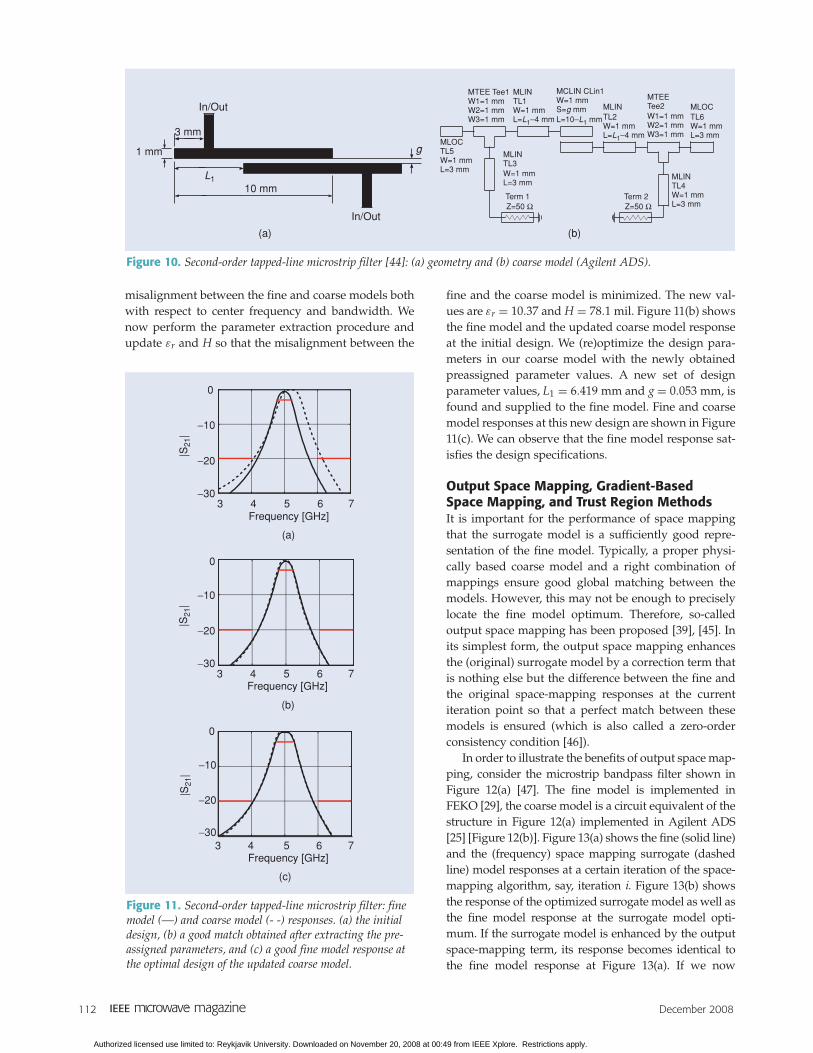
Consider the second-order tapped-line microstripfilter [44] shown in Figure 10(a). For the sake of sim-plicity we only use two design parameters, L1 and g asdefined in Figure 10(a). The fine model is simulated in

FEKO [29]. The design specifications are |S21| ≥ −3 dBfor 4.75 GHz ≤ ω ≤ 5.25 GHz, and |S21| ≤ –20 dB for3.0 GHz ≤ ω ≤ 4.0 GHz and 6.0 GHz ≤ ω ≤ 7.0 GHz.The coarse model shown in Figure 10(b) is the circuitequivalent of the structure in Figure 10(a), and isimplemented in Agilent ADS [25].

We want to optimize our filter using implicit spacemapping with the dielectric constant εr and height H ofthe substrate as preassigned parameters. Initial valuesof the parameters are 9.9 and 100 mil, respectively, forboth fine and coarse models. These parameters remainfixed in the fine model; however, we are going to tunethem in the coarse model, according to the implicitspace-mapping methodology.

The initial design, L1 = 6.977 mm and g = 0.060mm, is the optimal solution of the coarse model withrespect to our specifications. Figure 11(a) shows the fineand coarse model responses at the initial design. Notethat neither the coarse nor fine models satisfy thedesign specifications. Also, there is quite a significant

Figure 7. Interdigital filter initial design using parametersfrom [41]: the |S11| and |S21| responses of the fine modelsimulation (◦) versus the coarse model after the first para-meter extraction (—).

4 4.5 5 5.5 6–80

–70

–60

–50

–40

–30

–20

–10

0

Frequency [GHz]

|S21

| and

|S11

| (dB

)

Figure 6. Interdigital filter: coarse model. Capacitors areinserted between nonadjacent transmission lines.

C4 fF C5 fF C6 fF

C1 fF C2 fF C3 fF

Figure 9. The interdigital filter |S11| and |S21| passbanddetails of the fine model final simulation (◦) versus the sur-rogate model simulation (—).

4.9 5 5.1 5.2 5.3–0.4

–0.3

–0.2

–0.1

0

Frequency [GHz]

|S21

| (dB

)

Figure 8. The interdigital filter |S11| and |S21| responsesof the fine model final simulation (◦) versus the surrogatemodel (—).

4 4.5 5 5.5 6–80

–70

–60

–50

–40

–30

–20

–10

0

Frequency [GHz]

|S21

| and

|S11

| (dB

)


112 December 2008

misalignment between the fine and coarse models bothwith respect to center frequency and bandwidth. Wenow perform the parameter extraction procedure andupdate εr and H so that the misalignment between the

fine and the coarse model is minimized. The new val-ues are εr = 10.37 and H = 78.1 mil. Figure 11(b) showsthe fine model and the updated coarse model responseat the initial design. We (re)optimize the design para-meters in our coarse model with the newly obtainedpreassigned parameter values. A new set of designparameter values, L1 = 6.419 mm and g = 0.053 mm, isfound and supplied to the fine model. Fine and coarsemodel responses at this new design are shown in Figure11(c). We can observe that the fine model response sat-isfies the design specifications.

Output Space Mapping, Gradient-BasedSpace Mapping, and Trust Region MethodsIt is important for the performance of space mappingthat the surrogate model is a sufficiently good repre-sentation of the fine model. Typically, a proper physi-cally based coarse model and a right combination ofmappings ensure good global matching between themodels. However, this may not be enough to preciselylocate the fine model optimum. Therefore, so-calledoutput space mapping has been proposed [39], [45]. Inits simplest form, the output space mapping enhancesthe (original) surrogate model by a correction term thatis nothing else but the difference between the fine andthe original space-mapping responses at the currentiteration point so that a perfect match between thesemodels is ensured (which is also called a zero-orderconsistency condition [46]).

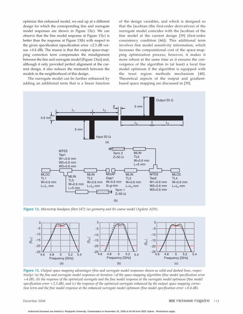
In order to illustrate the benefits of output space map-ping, consider the microstrip bandpass filter shown inFigure 12(a) [47]. The fine model is implemented inFEKO [29], the coarse model is a circuit equivalent of thestructure in Figure 12(a) implemented in Agilent ADS[25] [Figure 12(b)]. Figure 13(a) shows the fine (solid line)and the (frequency) space mapping surrogate (dashedline) model responses at a certain iteration of the space-mapping algorithm, say, iteration i. Figure 13(b) showsthe response of the optimized surrogate model as well asthe fine model response at the surrogate model opti-mum. If the surrogate model is enhanced by the outputspace-mapping term, its response becomes identical tothe fine model response at Figure 13(a). If we now

Figure 10. Second-order tapped-line microstrip filter [44]: (a) geometry and (b) coarse model (Agilent ADS).

1 mm

In/Out

g

L1

3 mm

In/Out

10 mmTerm 1Z=50 Ω

Term 2Z=50 Ω

MTEETee2W1=1 mmW2=1 mmW3=1 mm

MLINTL1W=1 mmL=L1–4 mm

MLINTL2W=1 mmL=L1–4 mm

MLOCTL5W=1 mmL=3 mm

MCLIN CLin1W=1 mmS=g mmL=10–L1 mm

MTEE Tee1W1=1 mmW2=1 mmW3=1 mm

MLINTL3W=1 mmL=3 mm

MLOCTL6W=1 mmL=3 mm

MLINTL4W=1 mmL=3 mm

(a) (b)

Figure 11. Second-order tapped-line microstrip filter: finemodel (—) and coarse model (- -) responses. (a) the initialdesign, (b) a good match obtained after extracting the pre-assigned parameters, and (c) a good fine model response atthe optimal design of the updated coarse model.

3 4 5 6 7

−10

−20

−30

0

Frequency [GHz]

(a)

3 4 5 6 7Frequency [GHz]

(b)

|S21

|

−10

−20

−30

0

|S21

|

3 4 5 6 7Frequency [GHz]

(c)

−10

−20

−30

0

|S21

|


December 2008 113

optimize this enhanced model, we end up at a differentdesign for which the corresponding fine and surrogatemodel responses are shown in Figure 13(c). We canobserve that the fine model response at Figure 13(c) isbetter than the response at Figure 13(b) with respect tothe given specification (specification error +2.3 dB ver-sus +0.4 dB). The reason is that the output space-map-ping correction term compensates the misalignmentbetween the fine and surrogate model [Figure 13(a)] and,although it only provided perfect alignment at the cur-rent design, it also reduces the mismatch between themodels in the neighborhood of this design.

The surrogate model can be further enhanced byadding an additional term that is a linear function

of the design variables, and which is designed sothat the Jacobian (the first-order derivatives) of thesurrogate model coincides with the Jacobian of thefine model at the current design [39] (first-orderconsistency condition [46]). This additional terminvolves fine model sensitivity information, whichincreases the computational cost of the space-map-ping optimization process; however, it makes itmore robust at the same time as it ensures the con-vergence of the algorithm to (at least) a local finemodel optimum if the algorithm is equipped withthe trust region methods mechanism [48].Theoretical aspects of the output and gradient-based space mapping are discussed in [39].

Figure 12. Microstrip bandpass filter [47]: (a) geometry and (b) coarse model (Agilent ADS).

0.6 mm

Output 50 Ω

Input 50 Ω

g

L3

L2L1

L4

5 mm

5 mm

Term 1Z=50 Ω

Term 2Z=50 Ω

MTEETee2W1=0.6 mmW2=0.6 mmW3=0.6 mm

MLINTL2W=0.6 mmL=L2 mm

MLINTL3W=0.6 mmL=L3 mm

MLOCTL1W=0.6 mmL=L1 mm

MGAPGap1W=0.6 mmS=g mm

MTEETee1W1=0.6 mmW2=0.6 mmW3=0.6 mm

MLINTL5W=0.6 mmL=5 mm

MLINTL6W=0.6 mmL=5 mm

MLOCTL4W=0.6 mmL=L4 mm

(a)

(b)

Figure 13. Output space mapping advantages (fine and surrogate model responses shown as solid and dashed lines, respec-tively): (a) the fine and surrogate model responses at iteration i of the space-mapping algorithm (fine model specification error+4 dB), (b) the response of the optimized surrogate and the fine model response at the surrogate model optimum (fine modelspecification error +2.3 dB), and (c) the response of the optimized surrogate enhanced by the output space mapping correc-tion term and the fine model response at the enhanced surrogate model optimum (fine model specification error +0.4 dB).

4.6 4.8 5 5.2 5.4−25

−20

−15

−10

−5

0 0 0

Frequency [GHz]

|S21

|

−25

−20

−15

−10

−5

|S21

|

−25

−20

−15

−10

−5

|S21

|

(a)

4.6 4.8 5 5.2 5.4Frequency [GHz]

(b)

4.6 4.8 5 5.2 5.4Frequency [GHz]

(c)


114 December 2008

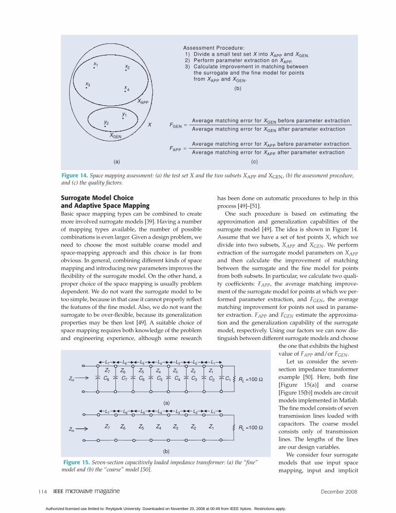
Surrogate Model Choiceand Adaptive Space MappingBasic space mapping types can be combined to createmore involved surrogate models [39]. Having a numberof mapping types available, the number of possiblecombinations is even larger. Given a design problem, weneed to choose the most suitable coarse model andspace-mapping approach and this choice is far fromobvious. In general, combining different kinds of spacemapping and introducing new parameters improves theflexibility of the surrogate model. On the other hand, aproper choice of the space mapping is usually problemdependent. We do not want the surrogate model to betoo simple, because in that case it cannot properly reflectthe features of the fine model. Also, we do not want thesurrogate to be over-flexible, because its generalizationproperties may be then lost [49]. A suitable choice ofspace mapping requires both knowledge of the problemand engineering experience, although some research

has been done on automatic procedures to help in thisprocess [49]–[51].

One such procedure is based on estimating theapproximation and generalization capabilities of thesurrogate model [49]. The idea is shown in Figure 14.Assume that we have a set of test points X, which wedivide into two subsets, XAPP and XGEN. We performextraction of the surrogate model parameters on XAPP

and then calculate the improvement of matchingbetween the surrogate and the fine model for pointsfrom both subsets. In particular, we calculate two quali-ty coefficients: FAPP, the average matching improve-ment of the surrogate model for points at which we per-formed parameter extraction, and FGEN, the averagematching improvement for points not used in parame-ter extraction. FAPP and FGEN estimate the approxima-tion and the generalization capability of the surrogatemodel, respectively. Using our factors we can now dis-tinguish between different surrogate models and choose

the one that exhibits the highestvalue of FAPP and/or FGEN.

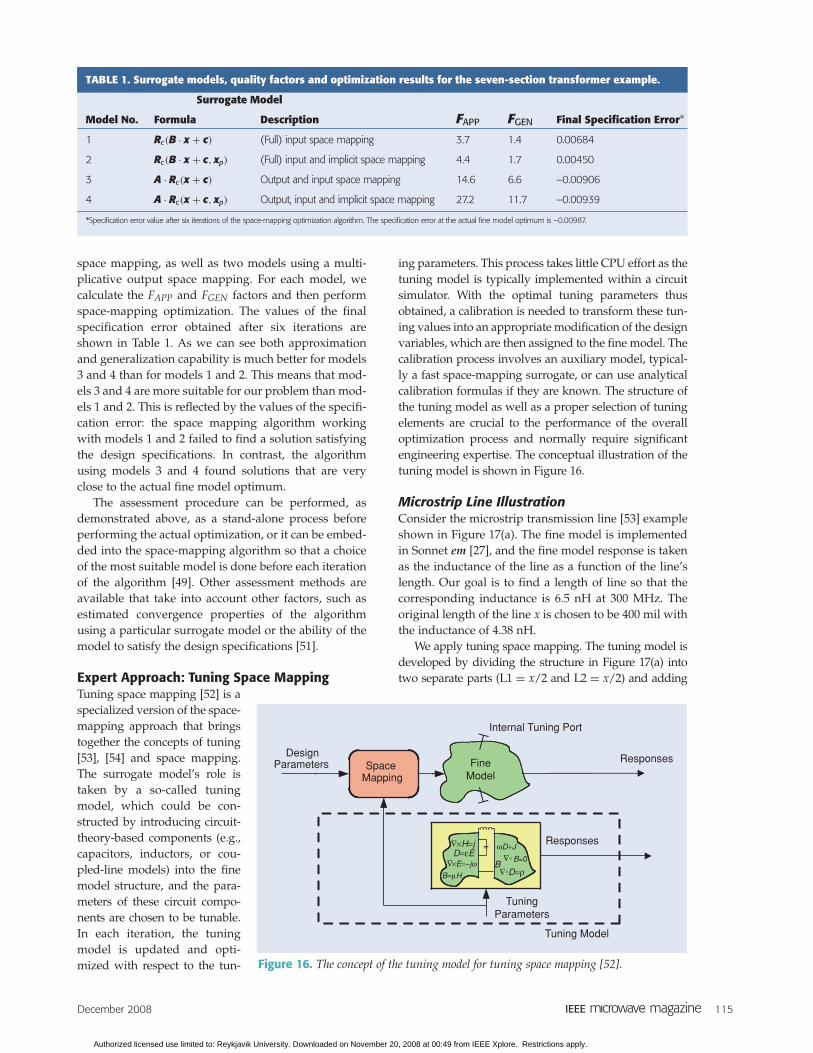
Let us consider the seven-section impedance transformerexample [50]. Here, both fine[Figure 15(a)] and coarse[Figure 15(b)] models are circuitmodels implemented in Matlab.The fine model consists of seventransmission lines loaded withcapacitors. The coarse modelconsists only of transmissionlines. The lengths of the linesare our design variables.

We consider four surrogatemodels that use input spacemapping, input and implicit

Figure 14. Space mapping assessment: (a) the test set X and the two subsets XAPP and XGEN, (b) the assessment procedure,and (c) the quality factors.

XGEN

XAPP

X

•

••

•

•

•x1 x2

x3 x4

y1

y2

(a)

Assessment Procedure: 1) Divide a small test set X into XAPP and XGEN. 2) Perform parameter extraction on XAPP. 3) Calculate improvement in matching between the surrogate and the fine model for points from XAPP and XGEN.

(b)

Average matching error for XGEN after parameter extraction

Average matching error for XAPP after parameter extraction

Average matching error for XAPP before parameter extraction

Average matching error for XGEN before parameter extractionFGEN =

FAPP =

(c)

Figure 15. Seven-section capacitively loaded impedance transformer: (a) the “fine”model and (b) the “coarse” model [50].

C3C4C5C6C7C8

L7 L6 L5 L4 L3 L2 L1

L7 L6 L5 L4 L3 L2 L1

RL =100 Ω

RL =100 Ω

Z7 Z6 Z5 Z4 Z3 Z2 Z1

C2 C1

Z7 Z6 Z5 Z4 Z3 Z2 Z1

(a)

Zin

Zin

(b)


December 2008 115

space mapping, as well as two models using a multi-plicative output space mapping. For each model, wecalculate the FAPP and FGEN factors and then performspace-mapping optimization. The values of the finalspecification error obtained after six iterations areshown in Table 1. As we can see both approximationand generalization capability is much better for models3 and 4 than for models 1 and 2. This means that mod-els 3 and 4 are more suitable for our problem than mod-els 1 and 2. This is reflected by the values of the specifi-cation error: the space mapping algorithm workingwith models 1 and 2 failed to find a solution satisfyingthe design specifications. In contrast, the algorithmusing models 3 and 4 found solutions that are veryclose to the actual fine model optimum.

The assessment procedure can be performed, asdemonstrated above, as a stand-alone process beforeperforming the actual optimization, or it can be embed-ded into the space-mapping algorithm so that a choiceof the most suitable model is done before each iterationof the algorithm [49]. Other assessment methods areavailable that take into account other factors, such asestimated convergence properties of the algorithmusing a particular surrogate model or the ability of themodel to satisfy the design specifications [51].

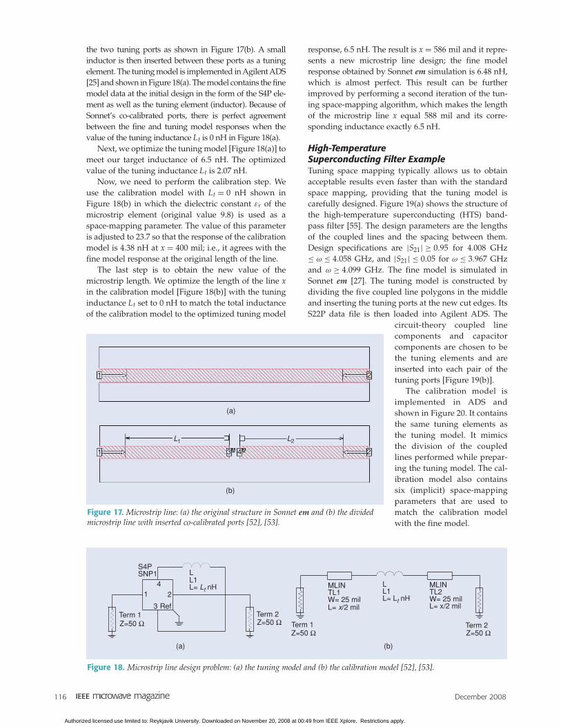
Expert Approach: Tuning Space MappingTuning space mapping [52] is aspecialized version of the space-mapping approach that bringstogether the concepts of tuning[53], [54] and space mapping.The surrogate model’s role istaken by a so-called tuningmodel, which could be con-structed by introducing circuit-theory-based components (e.g.,capacitors, inductors, or cou-pled-line models) into the finemodel structure, and the para-meters of these circuit compo-nents are chosen to be tunable.In each iteration, the tuningmodel is updated and opti-mized with respect to the tun-

ing parameters. This process takes little CPU effort as thetuning model is typically implemented within a circuitsimulator. With the optimal tuning parameters thusobtained, a calibration is needed to transform these tun-ing values into an appropriate modification of the designvariables, which are then assigned to the fine model. Thecalibration process involves an auxiliary model, typical-ly a fast space-mapping surrogate, or can use analyticalcalibration formulas if they are known. The structure ofthe tuning model as well as a proper selection of tuningelements are crucial to the performance of the overalloptimization process and normally require significantengineering expertise. The conceptual illustration of thetuning model is shown in Figure 16.

Microstrip Line IllustrationConsider the microstrip transmission line [53] exampleshown in Figure 17(a). The fine model is implementedin Sonnet em [27], and the fine model response is takenas the inductance of the line as a function of the line’slength. Our goal is to find a length of line so that thecorresponding inductance is 6.5 nH at 300 MHz. Theoriginal length of the line x is chosen to be 400 mil withthe inductance of 4.38 nH.

We apply tuning space mapping. The tuning model isdeveloped by dividing the structure in Figure 17(a) intotwo separate parts (L1 = x/2 and L2 = x/2) and adding

Figure 16. The concept of the tuning model for tuning space mapping [52].

FineModel

Space Mapping

Responses

Tuning Model

DesignParameters Responses

Tuning Parameters

B D=ρ

° ×E=−jωD=εE

B=μH

×H=j

Internal Tuning Port

ωD+J

B=0

Δ

Δ ΔΔ

°

TABLE 1. Surrogate models, quality factors and optimization results for the seven-section transformer example.

Surrogate Model

Model No. Formula Description FAPP FGEN Final Specification Error∗

1 Rc(B · x + c) (Full) input space mapping 3.7 1.4 0.00684

2 Rc(B · x + c, xp) (Full) input and implicit space mapping 4.4 1.7 0.00450

3 A · Rc(x + c) Output and input space mapping 14.6 6.6 –0.00906

4 A · Rc(x + c, xp) Output, input and implicit space mapping 27.2 11.7 –0.00939

*Specification error value after six iterations of the space-mapping optimization algorithm. The specification error at the actual fine model optimum is –0.00987.


116 December 2008

the two tuning ports as shown in Figure 17(b). A smallinductor is then inserted between these ports as a tuningelement. The tuning model is implemented in Agilent ADS[25] and shown in Figure 18(a). The model contains the finemodel data at the initial design in the form of the S4P ele-ment as well as the tuning element (inductor). Because ofSonnet’s co-calibrated ports, there is perfect agreementbetween the fine and tuning model responses when thevalue of the tuning inductance Lt is 0 nH in Figure 18(a).

Next, we optimize the tuning model [Figure 18(a)] tomeet our target inductance of 6.5 nH. The optimizedvalue of the tuning inductance Lt is 2.07 nH.

Now, we need to perform the calibration step. Weuse the calibration model with Lt = 0 nH shown inFigure 18(b) in which the dielectric constant εr of themicrostrip element (original value 9.8) is used as aspace-mapping parameter. The value of this parameteris adjusted to 23.7 so that the response of the calibrationmodel is 4.38 nH at x = 400 mil; i.e., it agrees with thefine model response at the original length of the line.

The last step is to obtain the new value of themicrostrip length. We optimize the length of the line xin the calibration model [Figure 18(b)] with the tuninginductance Lt set to 0 nH to match the total inductanceof the calibration model to the optimized tuning model

response, 6.5 nH. The result is x = 586 mil and it repre-sents a new microstrip line design; the fine modelresponse obtained by Sonnet em simulation is 6.48 nH,which is almost perfect. This result can be furtherimproved by performing a second iteration of the tun-ing space-mapping algorithm, which makes the lengthof the microstrip line x equal 588 mil and its corre-sponding inductance exactly 6.5 nH.

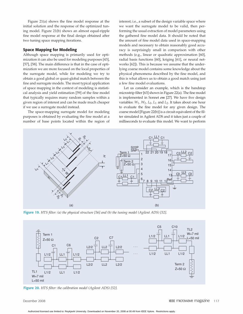
High-TemperatureSuperconducting Filter ExampleTuning space mapping typically allows us to obtainacceptable results even faster than with the standardspace mapping, providing that the tuning model iscarefully designed. Figure 19(a) shows the structure ofthe high-temperature superconducting (HTS) band-pass filter [55]. The design parameters are the lengthsof the coupled lines and the spacing between them.Design specifications are |S21| ≥ 0.95 for 4.008 GHz≤ ω ≤ 4.058 GHz, and |S21| ≤ 0.05 for ω ≤ 3.967 GHzand ω ≥ 4.099 GHz. The fine model is simulated inSonnet em [27]. The tuning model is constructed bydividing the five coupled line polygons in the middleand inserting the tuning ports at the new cut edges. ItsS22P data file is then loaded into Agilent ADS. The

circuit-theory coupled linecomponents and capacitorcomponents are chosen to bethe tuning elements and areinserted into each pair of thetuning ports [Figure 19(b)].

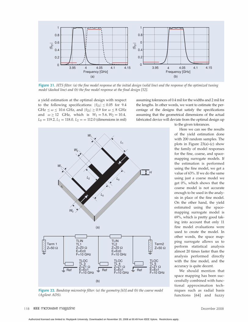
The calibration model isimplemented in ADS andshown in Figure 20. It containsthe same tuning elements asthe tuning model. It mimicsthe division of the coupledlines performed while prepar-ing the tuning model. The cal-ibration model also containssix (implicit) space-mappingparameters that are used tomatch the calibration modelwith the fine model.

Figure 18. Microstrip line design problem: (a) the tuning model and (b) the calibration model [52], [53].

Term 1Z=50 Ω

Term 2Z=50 Ω

S4PSNP1

1 2

3

4

Ref

LL1L= Lt nH

Term 1Z=50 Ω

Term 2Z=50 Ω

MLINTL1W= 25 milL= x/2 mil

LL1L= Lt nH

MLINTL2W= 25 milL= x/2 mil

(a) (b)

Figure 17. Microstrip line: (a) the original structure in Sonnet em and (b) the dividedmicrostrip line with inserted co-calibrated ports [52], [53].

(a)

(b)

1 2

1 3 4 2

L2L1

A A


December 2008 117

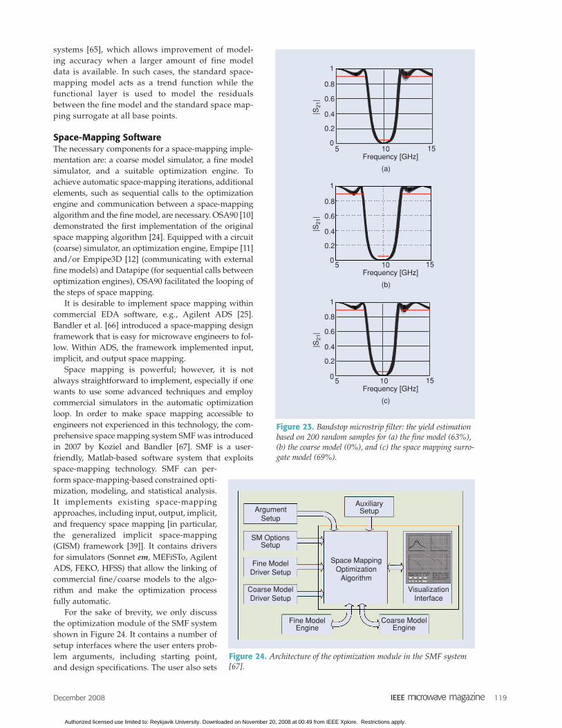
Figure 21(a) shows the fine model response at theinitial solution and the response of the optimized tun-ing model. Figure 21(b) shows an almost equal-ripplefine model response at the final design obtained aftertwo tuning space mapping iterations.

Space Mapping for ModelingAlthough space mapping is primarily used for opti-mization it can also be used for modeling purposes [43],[57], [58]. The main difference is that in the case of opti-mization we are more focused on the local properties ofthe surrogate model, while for modeling we try toobtain a good global or quasi-global match between thefine and surrogate models. The most typical applicationof space mapping in the context of modeling is statisti-cal analysis and yield estimation [59] of the fine modelthat typically requires many random samples within agiven region of interest and can be made much cheaperif we use a surrogate model instead.

The space-mapping surrogate model for modelingpurposes is obtained by evaluating the fine model at anumber of base points located within the region of

interest; i.e., a subset of the design variable space wherewe want the surrogate model to be valid, then per-forming the usual extraction of model parameters usingthe gathered fine model data. It should be noted thatthe amount of fine model data used in space-mappingmodels and necessary to obtain reasonably good accu-racy is surprisingly small in comparison with othermethods (e.g., linear or quadratic approximation [60],radial basis functions [60], kriging [61], or neural net-works [62]). This is because we assume that the under-lying coarse model contains some knowledge about thephysical phenomena described by the fine model, andthis is what allows us to obtain a good match using justa few fine model evaluations.

Let us consider an example, which is the bandstopmicrostrip filter [63] shown in Figure 22(a). The fine modelis implemented in Sonnet em [27]. We have five designvariables: W1, W2, L0, L1 and L2. It takes about one hourto evaluate the fine model for any given design. Thecoarse model [Figure 22(b)] is a circuit equivalent of the fil-ter simulated in Agilent ADS and it takes just a couple ofmilliseconds to evaluate this model. We want to perform

Figure 19. HTS filter: (a) the physical structure [56] and (b) the tuning model (Agilent ADS) [52].

S

2

S

1

S

3

S

1L 0L 1

L 0

L 2

L 1

L 2

L 3

S

2

W

H

S22PSNP1

LL1.

.

.

.

1

2

3

4

5

67 8 9 10 11 12

17

16

15

14

13

22 21 20 19 18

RefC1 C1

.

.

.

.

C2 C2LL2

.

.

.

.

C3 C3LL3

.

.

.

.

C2 C2LL2

.

.

.

.

C1 C1LL1

Term 1Z=50 Ω

Term 2Z=50 Ω

(a) (b)

εr

Figure 20. HTS filter: the calibration model (Agilent ADS) [52].

Term 1

Z=50 Ω

Term 2

Z=50 ΩTL1

W=7 milL=50 mil

.

.

.

.

.

.

.

.

.

.

.

.. . .

. . .

TL2W=7 milL=50 mil

C1 C6

L1/2 LL1 L1/2

L1/2 LL1 L1/2

C2 C7

L2/2 LL2 L2/2

L2/2 LL2 L2/2

C5 C10

L1/2 LL1 L1/2

L1/2 LL1 L1/2


118 December 2008

a yield estimation at the optimal design with respectto the following specifications: |S21| ≤ 0.05 for 9.4GHz ≤ ω ≤ 10.6 GHz, and |S21| ≥ 0.9 for ω ≤ 8 GHzand ω ≥ 12 GHz, which is W1 = 5.6, W2 = 10.4,

L0 = 119.2, L1 = 118.0, L2 = = 112.0 (dimensions in mil)

assuming tolerances of 0.4 mil for the widths and 2 mil forthe lengths. In other words, we want to estimate the per-centage of the designs that satisfy the specificationsassuming that the geometrical dimensions of the actualfabricated device will deviate from the optimal design up

to the given tolerances. Here we can see the results

of the yield estimation donewith 200 random samples. Theplots in Figure 23(a)–(c) showthe family of model responsesfor the fine, coarse, and space-mapping surrogate models. Ifthe estimation is performedusing the fine model, we get avalue of 63%. If we do the sameusing just a coarse model weget 0%, which shows that thecoarse model is not accurateenough to be used in the analy-sis in place of the fine model.On the other hand, the yieldestimated using the space-mapping surrogate model is69%, which is pretty good tak-ing into account that only 11fine model evaluations wereused to create the model. Inother words, the space map-ping surrogate allows us toperform statistical analysisalmost 20 times faster than theanalysis performed directlywith the fine model, and theaccuracy is quite decent.

We should mention thatspace mapping has been suc-cessfully combined with func-tional approximation tech-niques such as radial basisfunctions [64] and fuzzy

Figure 21. HTS filter: (a) the fine model response at the initial design (solid line) and the response of the optimized tuningmodel (dashed line) and (b) the fine model response at the final design [52].

3.95 4 4.05 4.1 4.150

0.2

0.4

0.6

0.8

1

Frequency [GHz]

|S21

|

3.95 4 4.05 4.1 4.150

0.2

0.4

0

0.8

1

Frequency [GHz]

|S21

|

(a) (b)

Figure 22. Bandstop microstrip filter: (a) the geometry [63] and (b) the coarse model(Agilent ADS).

εr

W1

W2

W0

L1

H

L2

W1

L0

L0

Term 1Z=50 Ω

Term2Z=50 Ω

TLINTL1Z=Z0 ΩE=Ec0F=10 GHz

Ref

TLINTL2Z=Z0 ΩE=Ec0F=10 GHz

TLOCTL 3Z=Z1 ΩE=Ec1F=10 GHz



Ref Ref

(a)

(b)


December 2008 119

systems [65], which allows improvement of model-ing accuracy when a larger amount of fine modeldata is available. In such cases, the standard space-mapping model acts as a trend function while thefunctional layer is used to model the residualsbetween the fine model and the standard space map-ping surrogate at all base points.

Space-Mapping SoftwareThe necessary components for a space-mapping imple-mentation are: a coarse model simulator, a fine modelsimulator, and a suitable optimization engine. Toachieve automatic space-mapping iterations, additionalelements, such as sequential calls to the optimizationengine and communication between a space-mappingalgorithm and the fine model, are necessary. OSA90 [10]demonstrated the first implementation of the originalspace mapping algorithm [24]. Equipped with a circuit(coarse) simulator, an optimization engine, Empipe [11]and/or Empipe3D [12] (communicating with externalfine models) and Datapipe (for sequential calls betweenoptimization engines), OSA90 facilitated the looping ofthe steps of space mapping.

It is desirable to implement space mapping withincommercial EDA software, e.g., Agilent ADS [25].Bandler et al. [66] introduced a space-mapping designframework that is easy for microwave engineers to fol-low. Within ADS, the framework implemented input,implicit, and output space mapping.

Space mapping is powerful; however, it is notalways straightforward to implement, especially if onewants to use some advanced techniques and employcommercial simulators in the automatic optimizationloop. In order to make space mapping accessible toengineers not experienced in this technology, the com-prehensive space mapping system SMF was introducedin 2007 by Koziel and Bandler [67]. SMF is a user-friendly, Matlab-based software system that exploitsspace-mapping technology. SMF can per-form space-mapping-based constrained opti-mization, modeling, and statistical analysis.It implements existing space-mappingapproaches, including input, output, implicit,and frequency space mapping [in particular,the generalized implicit space-mapping(GISM) framework [39]]. It contains driversfor simulators (Sonnet em, MEFiSTo, AgilentADS, FEKO, HFSS) that allow the linking ofcommercial fine/coarse models to the algo-rithm and make the optimization processfully automatic.

For the sake of brevity, we only discussthe optimization module of the SMF systemshown in Figure 24. It contains a number ofsetup interfaces where the user enters prob-lem arguments, including starting point,and design specifications. The user also sets

Figure 23. Bandstop microstrip filter: the yield estimationbased on 200 random samples for (a) the fine model (63%),(b) the coarse model (0%), and (c) the space mapping surro-gate model (69%).

(a)

5 10 150

0.8

0.6

0.4

0.2

1

Frequency [GHz]

(b)

5 10 15Frequency [GHz]

(c)

5 10 15Frequency [GHz]

|S21

|

0

0.8

0.6

0.4

0.2

1

|S21

|

0

0.8

0.6

0.4

0.2

1

|S21

|

Figure 24. Architecture of the optimization module in the SMF system[67].

ArgumentSetup

AuxiliarySetup

SM OptionsSetup

Fine ModelDriver Setup

Fine ModelEngine

Space MappingOptimization

Algorithm

Coarse ModelDriver Setup

Coarse ModelEngine

VisualizationInterface


120 December 2008

up the type of space mapping to be used, specifies ter-mination conditions, parameter extraction options,and optional constraints. The next step is to link thefine and coarse models to SMF by setting up the data(e.g., simulator input files and design variable identi-fication data) that will be used to create model drivers.The drivers are later used to evaluate fine/coarsemodels for any required design variable values.Having done the setup, the user starts the executioninterface, which allows us to run the space-mappingoptimization algorithm and visualize the results,including model responses, specification error plots,and convergence plots.

Figure 25 shows the flowchart of the space-map-ping optimization process. First, the user needs to setup whatever is necessary as described before includingthe design specifications and space-mapping type onewants to use as well as the termination condition forthe algorithm. The next step is to link fine/coarse mod-els to the system by providing necessary data about thesimulator, design variables, and initial design. The ini-tial step of space mapping optimization is typically theoptimization of the coarse model. This can be doneusing a dedicated interface and the coarse model opti-mal solution can be then used as a starting point for thespace-mapping optimization. The actual space-map-ping optimization is performed in the execution inter-face, which contains the response plot, specificationerror plot, convergence plots, a panel with correspond-ing numeric values, as well as a number of controls to

run, stop, reset the algorithm, and review it iteration byiteration. The optimization process is fully automatic;however, the user can intervene if necessary.

DiscussionDistinction [68] should be made between space-map-ping optimization and optimization based on function-al approximations using polynomials [60], radial basisfunctions [60], kriging [61], etc. The latter methodsestablish a localized approximation of fine modelresponses using fine model simulations. Such approxi-mations are typically updated using new fine modelpoints. On the other hand, for a small investment in finemodel simulations, space mapping exploits an underly-ing coarse model (knowledge) that is physically basedand capable of accurately simulating the system underconsideration over a wide range of parameter values.The surrogate is updated iteratively.

Knowledge-based neural network models [69]and so-called neural space mapping [63] also takeadvantage of a coarse model to expand the region ofvalidity beyond the range of the training data and/orto reduce the number of data points required in thetraining process.

Advantages of space mapping can be summarized asfollows. It provides an efficient (typically only a few iter-ations are required) optimization method for expensivemodels (e.g., EM-simulation-based models). Typically, itdoes not require fine model derivatives. Space-map-ping-based interpolation makes a continuous model

Figure 25. Flowchart of the space-mapping optimization in the SMF system. The process includes setup, linking of thefine/coarse models to the system, coarse model optimization, and automatic space-mapping optimization.

Setup Linking Fine/Coarse Models

Space Mapping Optimization

Coarse Model Optimization


December 2008 121

available on a discrete subset of the design space [70].Fast surrogate optimization allows a larger number ofdesign parameters to be considered [31], [71], whichimplies a better chance of obtaining a good design. Agood surrogate model remains useful after the designprocess is completed.

SummaryMicrowave CAD has its roots in the 1960s [1]. Itspractice saw the enrichment of circuit-based modellibraries, advances in EM and circuit simulationaccuracy, and the refinement of microwave optimiza-tion technology. In 1994 [24], space mappingemerged: a powerful yet simple mathematicallybased technology that takes advantage of progress inthe aforementioned key areas. Space mapping hassince developed into an approach of choice for EM-based design. In this article, we provided a generalframework for the space-mapping optimization con-cept. We illustrated space-mapping optimizationthrough a simple bandstop filter. We demonstratedthe robustness of the technique by performing anaccurate design of an interdigital filter. We reviewedstate-of-the-art developments in space mapping thatfeature implicit space mapping, output space map-ping, gradient-based space mapping as well as trustregion methods; surrogate model choice and adap-tive space mapping; tuning space mapping; andspace mapping for device modeling. We reviewedimplementation techniques and demonstrated theSMF space-mapping software package.

AcknowledgmentsThis work was supported in part by the NaturalSciences and Engineering Research Council of Canadaunder Grants RGPIN7239-06, and STPGP336760-06,and by Bandler Corporation.

We thank Sonnet Software, Inc., Syracuse, NewYork, for em, and Agilent Technologies, Santa Rosa,California, for ADS. Jim Rautio of Sonnet Software isthanked for help on novel uses of his software.

We would like to acknowledge various technical col-laborators who helped shape our research, including JieMeng, Mohamed H. Bakr, and Natalia K. Nikolova ofMcMaster University, Canada; José Rayas-Sánchez ofITESO, Guadalajara, Mexico; Qi-Jun Zhang, CarletonUniversity, Canada; and K. Madsen, TechnicalUniversity of Denmark, Lyngby, Denmark.

References[1] G.C. Temes and D.A. Calahan, “Computer-aided network opti-

mization the state-of-the-art,” Proc. IEEE, vol. 55, no. 11, pp.1832–1863, Nov. 1967.

[2] J.W. Bandler, “Optimization methods for computer-aideddesign,” IEEE Trans. Microwave Theory Tech., vol. MTT-17, no. 8,pp. 533–552, Aug. 1969.

[3] J.W. Bandler, “Computer-aided circuit optimization,” in ModernFilter Theory and Design, G.C. Temes and S. K. Mitra, Eds. NewYork: Wiley, pp. 211–271, 1973.

[4] G.E. Brehm, “Multifunction MMIC history from a process tech-nology perspective,” IEEE Trans. Microwave Theory Tech., vol. 38,no. 9, pp. 1164–1170, Sept. 1990.

[5] J.W. Bandler, S.H. Chen, S. Daijavad, W. Kellermann, M. Renault,and Q.J. Zhang, “Large scale minimax optimization of microwavemultiplexers,” in Proc. European Microwave Conf., Dublin, Ireland,Sept. 1986, pp. 435–440.

[6] J.W. Bandler and S.H. Chen, “Circuit optimization: the state of the art,”IEEE Trans. Microwave Theory Tech., vol. 36, no. 2, pp. 424–443, Feb. 1988.

[7] J.W. Bandler and A.E. Salama, “Functional approach tomicrowave postproduction tuning,” IEEE Trans. Microwave TheoryTech., vol. MTT-33, no. 4, pp. 302–310, Apr. 1985.

[8] P-N Designs, Inc., “History of microwave software.” [Online].Available: http://www.microwaves101.com/encyclopedia/historyCAD.cfm

[9] J.W. Bandler, P.C. Liu, and H. Tromp, “A nonlinear programmingapproach to optimal design centering, tolerancing and tuning,”IEEE Trans. Circuits Syst., vol. CAS-23, no. 3, pp. 155–165, Mar. 1976.

[10] OSA90/hope™, version 4.0, User’s Manual, August 1997,Optimization Systems Associates Inc. (now Agilent Technologies),Dundas, Ontario, Canada.

[11] Empipe™, version 4.0, User’s Manual, July 1997, OptimizationSystems Associates Inc. (now Agilent Technologies), Dundas,Ontario, Canada.

[12] Empipe3D™, version 4.0, User’s Manual, June 1997,Optimization Systems Associates Inc. (now Agilent Technologies),Dundas, Ontario, Canada.

[13] J.W. Bandler, R.M. Biernacki, S.H. Chen, P.A. Grobelny, and S. Ye,“Yield-driven electromagnetic optimization via multilevel multi-dimensional models,” IEEE Trans. Microwave Theory Tech., vol. 41,no. 12, pp. 2269–2278, Dec. 1993.

[14] J.W. Bandler, R.M. Biernacki, and S.H. Chen, “Parameterizationof arbitrary geometrical structures for automated electromagneticoptimization,” Int. J. RF Microwave CAE, vol. 9, no. 2, pp. 73–85,Feb. 1999.

[15] J.W. Bandler, R.M. Biernacki, S.H. Chen, D.G. Swanson, Jr., andS. Ye, “Microstrip filter design using direct EM field simulation,”IEEE Trans. Microwave Theory Tech., vol. 42, no. 7, pp. 1353–1359,July 1994.

[16] J.W. Bandler, R.M. Biernacki, S.H. Chen, W.J. Getsinger, P.A.Grobelny, C. Moskowitz, and S.H. Talisa, “Electromagnetic design ofhigh-temperature superconducting microwave filters,” Int. J.Microwave Millimeter-Wave CAE, vol. 5, no. 5, pp. 331–343, Sept. 1995.

[17] J.W. Bandler, R.M. Biernacki, S.H. Chen, L.W. Hendrick, and D.Omeragic´, “Electromagnetic optimization of 3-D structures,” IEEETrans. Microwave Theory Tech., vol. 45, no. 5, pp. 770–779, May 1997.

[18] D.G. Swanson, Jr., “Optimizing a microstrip bandpass filterusing electromagnetics,” Int. J. Microwave Millimeter-Wave CAE,vol. 5, no. 5, pp. 344–351, Sep. 1995.

[19] D.G. Swanson, Jr., “Computer aided design of passive compo-nents,” in The RF and Microwave Handbook, M. Golio, Ed. BocaRaton, FL: CRC Press, 2000, pp. 8-34–8-44.

[20] D.G. Swanson, Jr. and W.J.R. Hoefer, Microwave Circuit ModelingUsing Electromagnetic Field Simulation. Norwood, MA: ArtechHouse, 2003.

[21] http://www.bandler.com/mileston2.htm[22] A. Dounavis, E. Gad, R. Achar, and M.S. Nakhla, “Passive model

reduction of multiport distributed interconnects,” IEEE Trans.Microwave Theory Tech., vol. 48, no. 12, pp. 2325–2334, Dec. 2000.

[23] A.H. Zaabab, Q.J. Zhang, and M.S. Nakhla, “A neural network mod-eling approach to circuit optimization and statistical design,” IEEETrans. Microwave Theory Tech., vol. 43, no. 6, pp. 1349–1358, June 1995.

[24] J.W. Bandler, R.M. Biernacki, S.H. Chen, P.A. Grobelny, andR.H. Hemmers, “Space mapping technique for electromagneticoptimization,” IEEE Trans. Microwave Theory Tech., vol. 42, no. 12,pp. 2536–2544, Dec. 1994.

[25] Agilent ADS 2005A, Agilent Technologies, Santa Rosa, CA USA.[26] Agilent Momentum 2005A, Agilent Technologies, Santa Rosa,

CA USA.[27] Sonnet em Version 11.52, Sonnet Software, Inc., North Syracuse,

NY USA.


122 December 2008

[28] Ansoft HFSS Version 10.1, Ansoft Corporation, Pittsburgh, PAUSA.

[29] FEKO User’s Manual, Suite 4.2, June 2004, EM Software &Systems-S.A. (Pty) Ltd., Stellenbosch, South Africa. Available:http://www.feko.info.

[30] MEFiSTo-3D Pro, Version 3.0, Faustus Scientific Corp., Victoria,BC, Canada.

[31] Q.S. Cheng, J.W. Bandler, and S. Koziel, “Combining coarse andfine models for optimal design,” IEEE Microwave Mag., vol. 9, no.1, pp. 79–88, Feb. 2008.

[32] A.J. Booker, J.E. Dennis, Jr., P.D. Frank, D.B. Serafini, V.Torczon, and M.W. Trosset, “A rigorous framework for opti-mization of expensive functions by surrogates,” StructuralOptimization, vol. 17, no. 1, pp. 1–13, Feb. 1999.

[33] A.M. Pavio, “The electromagnetic optimization of microwavecircuits using companion models,” presented at Workshop onNovel Methods for Device Modeling and Circuit CAD, IEEEMTT-S Int. Microwave Symp., Anaheim, CA, 1999.

[34] D. Swanson and G. Macchiarella, “Microwave filter design by synthesisand optimization,” IEEE Microwave Mag., vol. 8, no. 2, pp. 55–69, Apr. 2007.

[35] D. Swanson, Jr., “Narrow-band microwave filter design,” IEEEMicrowave Mag., vol. 8, no. 5, pp. 105–114, Oct. 2007.

[36] R.J. Cameron and M. Yu, “Design of manifold coupled multi-plexers,” IEEE Microwave Mag., vol. 8, no. 5, pp. 46–59, Oct. 2007.

[37] J.W. Bandler, A.S. Mohamed, and M.H. Bakr, “TLM-based mod-eling and design exploiting space mapping,” IEEE Trans.Microwave Theory Tech., vol. 53, no. 9, pp. 2801–2811, Sept. 2005.

[38] J.C. Rautio, “EM-component-based design of planar circuits,”IEEE Microwave Mag., vol. 8, no. 4, pp. 79–90, Aug. 2007.

[39] S. Koziel, J.W. Bandler, and K. Madsen, “A space mapping frameworkfor engineering optimization: theory and implementation,” IEEE Trans.Microwave Theory Tech., vol. 54, no. 10, pp. 3721–3730, Oct. 2006.

[40] Matlab, Version 7.1, The MathWorks, Inc., Natick, MA, 2005.[41] J.W. Bandler, R.M. Biernacki, S.H. Chen, and Y.F. Huang, “Design

optimization of interdigital filters using aggressive space mappingand decomposition,” IEEE Trans. Microwave Theory Tech., vol. 45,no. 5, pp. 761–769, May 1997.

[42] J.W. Bandler, Q.S. Cheng, N.K. Nikolova, and M.A. Ismail,“Implicit space mapping optimization exploiting preassignedparameters,” IEEE Trans. Microwave Theory Tech., vol. 52, no. 1,pp. 378–385, Jan. 2004.

[43] Q.S. Cheng and J.W. Bandler, “An implicit space mapping tech-nique for component modeling,” in Proc. 36th European MicrowaveConf., Manchester, UK, Sept. 2006, pp. 458–461.

[44] A. Manchec, C. Quendo, J.-F. Favennec, E. Rius, and C. Person,“Synthesis of capacitive-coupled dual-behavior resonator(CCDBR) filters,” IEEE Trans. Microwave Theory Tech., vol. 54, no. 6,pp. 2346–2355, June 2006.

[45] J.W. Bandler, Q.S. Cheng, D.H. Gebre-Mariam, K. Madsen, F.Pedersen, and J. Søndergaard, “EM-based surrogate modeling anddesign exploiting implicit, frequency and output space map-pings,” in IEEE MTT-S Int. Microwave Symp. Dig., Philadelphia,PA, June 2003, pp. 1003–1006.

[46] N.M. Alexandrov and R.M. Lewis, “An overview of first-ordermodel management for engineering optimization,” OptimizationEng., vol. 2, no. 4, pp. 413–430, Dec. 2001.

[47] A. Hennings, E. Semouchkina, A. Baker, and G. Semouchkin,“Design optimization and implementation of bandpass filters withnormally fed microstrip resonators loaded by high-permittivitydielectric,” IEEE Trans. Microwave Theory and Tech., vol. 54, no. 3,pp. 1253–1261, Mar. 2006.

[48] A.R. Conn, N.I.M. Gould, and P.L. Toint, Trust Region Methods,MPS-SIAM Series on Optimization. Philadelphia, PA: Society forIndustrial and Applied Mathmatics, 2000.

[49] S. Koziel and J.W. Bandler, “Space-mapping optimization withadaptive surrogate model,” IEEE Trans. Microwave Theory Tech.,vol. 55, no. 3, pp. 541–547, Mar. 2007.

[50] S. Koziel and J.W. Bandler, “Coarse and surrogate modelassessment for engineering design optimization with spacemapping,” IEEE MTT-S Int. Microwave Symp. Dig., Honolulu, HI,June 2007, pp. 107–110.

[51] S. Koziel, J.W. Bandler, and K. Madsen, “Quality assessment ofcoarse models and surrogates for space mapping optimization,”Optimization Eng., vol. 9, no. 4, pp. 375–391, Dec. 2008.

[52] J. Meng, S. Koziel, J.W. Bandler, M.H. Bakr, and Q.S. Cheng,“Tuning space mapping: A novel technique for engineering designoptimization,” in IEEE MTT-S Int. Microwave Symp. Dig., Atlanta,GA, June 2008, pp. 991–994.

[53] J.C. Rautio, “RF design closure—companion modeling and tun-ing methods,” IEEE MTT-S IMS Workshop: Microwave componentdesign using space mapping technology, San Francisco, CA, 2006.

[54] D.G. Swanson and R.J. Wenzel, “Fast analysis and optimizationof combline filters using FEM,” in IEEE MTT-S Int. MicrowaveSymp. Dig., Boston, MA, July 2001, pp. 1159–1162.

[55] J.W. Bandler, R.M. Biernacki, S.H. Chen, R.H. Hemmers, and K.Madsen, “Electromagnetic optimization exploiting aggressivespace mapping,” IEEE Trans. Microwave Theory Tech., vol. 43, no. 12,pp. 2874–2882, Dec. 1995.

[56] J.W. Bandler, R.M. Biernacki, S.H. Chen, W.J. Getsinger, P.A.Grobelny, C. Moskowitz, and S.H. Talisa, “Electromagnetic designof high-temperature superconducting microwave filters,” Int. J. RFMicrowave CAE, vol. 5, no. 5, pp. 331–343, Sept. 1995.

[57] S. Koziel, J.W. Bandler, A.S. Mohamed, and K. Madsen,“Enhanced surrogate models for statistical design exploiting spacemapping technology,” in IEEE MTT-S Int. Microwave Symp. Dig.,Long Beach, CA, June 2005, pp. 1609–1612.

[58] S. Koziel, J.W. Bandler, and K. Madsen, “Theoretical justificationof space-mapping-based modeling utilizing a data base and on-demand parameter extraction,” IEEE Trans. Microwave TheoryTech., vol. 54, no. 12, pp. 4316–4322, Dec. 2006.

[59] J.E. Rayas-Sánchez and V. Gutiérrez-Ayala, “EM-based MonteCarlo analysis and yield prediction of microwave circuits usinglinear-input neural-output space mapping,” IEEE Trans. MicrowaveTheory Tech., vol. 54, pp. 4528–4537, Dec. 2006.

[60] T.W. Simpson, J.D. Peplinski, P.N. Koch, and J.K. Allen, “Metamodelsfor computer-based engineering design: Survey and recommenda-tions,” Eng. Comput., vol. 17, no. 2, pp. 129–150, July 2001.

[61] T.W. Simpson, T.M. Maurey, J.J. Korte, and F. Mistree, “Kriging mod-els for global approximation in simulation-based multidisciplinarydesign optimization,” AIAA J., vol. 39, no. 12, pp. 2233–2241, Dec. 2001.

[62] J.E. Rayas-Sánchez, “EM-based optimization of microwave cir-cuits using artificial neural networks: the state of the art,” IEEETrans. Microwave Theory Tech., vol. 52, no. 1, pp. 420–435, Jan. 2004.

[63] M.H. Bakr, J.W. Bandler, M.A. Ismail, J.E. Rayas-Sánchez, and Q.J. Zhang,“Neural space mapping optimization for EM-based design,” IEEE Trans.Microwave Theory Tech., vol. 48, no. 12, pp. 2307–2315, Dec. 2000.

[64] S. Koziel and J.W. Bandler, “Microwave device modeling usingspace-mapping and radial basis functions,” in IEEE MTT-S Int.Microwave Symp. Dig., Honolulu, HI, June 2007, pp. 799–802.

[65] S. Koziel and J.W. Bandler, “A space-mapping approach tomicrowave device modeling exploiting fuzzy systems,” IEEETrans. Microwave Theory and Tech., vol. 55, no. 12, pp. 2539–2547,Dec. 2007.

[66] J.W. Bandler, Q.S. Cheng, D.M. Hailu, and N.K. Nikolova, “Aspace-mapping design framework,” IEEE Trans. Microwave TheoryTech., vol. 52, no. 11, pp. 2601–2610, Nov. 2004.

[67] S. Koziel and J.W. Bandler, “SMF: A user-friendly softwareengine for space-mapping-based engineering design optimiza-tion,” in Proc. Int. Symp. Signals, Systems and Electronics, URSIISSSE 2007, Montreal, Canada, July 2007, pp. 157–160.

[68] M.H. Bakr, J.W. Bandler, K. Madsen, and J. Søndergaard, “Reviewof the space mapping approach to engineering optimization andmodeling,” Optimization Eng., vol. 1, no. 3, pp. 241–276, Sept. 2000.

[69] F. Wang and Q.J. Zhang, “Knowledge based neural models formicrowave design,” IEEE Trans. Microwave Theory Tech., vol. 45,no. 12, pp. 2333–2343, Dec. 1997.

[70] S. Koziel, J.W. Bandler, and K. Madsen, ”Space-mapping basedinterpolation for engineering optimization,” IEEE Trans.Microwave Theory and Tech., vol. 54, no. 6, pp. 2410–2421, June 2006.

[71] Q.S. Cheng, J.W. Bandler, and J.E. Rayas-Sánchez, “Tuning-aidedimplicit space mapping,” Int. J. RF Microwave CAE, vol. 18, no. 5,pp. 445–453, Sept. 2008.


slawomir koziel, qingsha s. cheng, and john w. bandler ieomc.ru.is/eoml_pdf/paper_1.pdf · digital...

Documents