NBER WORKING PAPER SERIES

SKILLS, TASKS AND TECHNOLOGIES:IMPLICATIONS FOR EMPLOYMENT AND EARNINGS

Daron AcemogluDavid Autor

Working Paper 16082http://www.nber.org/papers/w16082

NATIONAL BUREAU OF ECONOMIC RESEARCH1050 Massachusetts Avenue

Cambridge, MA 02138June 2010

We thank Amir Kermani for outstanding research assistance and Melanie Wasserman for persistent,meticulous and ingenious work on all aspects of the chapter. We are indebted to Arnaud Costinot andDavid Dorn for insightful comments and suggestions, and to David Dorn, Nicole Fortin, and MaartenGoos for generous assistance with data. Autor acknowledges support from the National Science Foundation(CAREER award SES-0239538).The views expressed herein are those of the authors and do not necessarilyreflect the views of the National Bureau of Economic Research.

NBER working papers are circulated for discussion and comment purposes. They have not been peer-reviewed or been subject to the review by the NBER Board of Directors that accompanies officialNBER publications.

© 2010 by Daron Acemoglu and David Autor. All rights reserved. Short sections of text, not to exceedtwo paragraphs, may be quoted without explicit permission provided that full credit, including © notice,is given to the source.

Skills, Tasks and Technologies: Implications for Employment and EarningsDaron Acemoglu and David AutorNBER Working Paper No. 16082June 2010JEL No. J20,J23,J24,J30,O31,O33

ABSTRACT

A central organizing framework of the voluminous recent literature studying changes in the returnsto skills and the evolution of earnings inequality is what we refer to as the canonical model, whichelegantly and powerfully operationalizes the supply and demand for skills by assuming two distinctskill groups that perform two different and imperfectly substitutable tasks or produce two imperfectlysubstitutable goods. Technology is assumed to take a factor-augmenting form, which, by complementingeither high or low skill workers, can generate skill biased demand shifts. In this paper, we argue thatdespite its notable successes, the canonical model is largely silent on a number of central empiricaldevelopments of the last three decades, including: (1) significant declines in real wages of low skillworkers, particularly low skill males; (2) non-monotone changes in wages at different parts of theearnings distribution during different decades; (3) broad-based increases in employment in high skilland low skill occupations relative to middle skilled occupations (i.e., job 'polarization'); (4) rapid diffusionof new technologies that directly substitute capital for labor in tasks previously performed by moderately-skilled workers; and (5) expanding offshoring opportunities, enabled by technology, which allow foreignlabor to substitute for domestic workers in specific tasks. Motivated by these patterns, we argue thatit is valuable to consider a richer framework for analyzing how recent changes in the earnings andemployment distribution in the United States and other advanced economies are shaped by the interactionsamong worker skills, job tasks, evolving technologies, and shifting trading opportunities. We proposea tractable task-based model in which the assignment of skills to tasks is endogenous and technicalchange may involve the substitution of machines for certain tasks previously performed by labor. Wefurther consider how the evolution of technology in this task-based setting may be endogenized. Weshow how such a framework can be used to interpret several central recent trends, and we also suggestfurther directions for empirical exploration.

Daron AcemogluDepartment of EconomicsMIT, E52-380B50 Memorial DriveCambridge, MA 02142-1347and CIFARand also NBERdaron@mit.edu

David AutorDepartment of EconomicsMIT, E52-37150 Memorial DriveCambridge, MA 02142-1347and NBERdautor@mit.edu

1 Introduction

The changes in the distribution of earnings and the returns to college over the last several decades in

the U.S. labor market have motivated a large literature investigating the relationship between technical

change and wages. The starting point of this literature is the observation that the return to skills, for

example as measured by the relative wages of college graduate workers to high school graduates, has

shown a tendency to increase over multiple decades despite the large secular increase in the relative

supply of college educated workers. This suggests that concurrent with the increase in the supply of

skills, there has been an increase in the (relative) demand for skills. Following Tinbergen’s pioneering

(1974, 1975) work, the relative demand for skills is then linked to technology, and in particular to the

skill bias of technical change. This perspective emphasizes that the return to skills (and to college)

is determined by a race between the increase in the supply of skills in the labor market and technical

change, which is assumed to be skill biased, in the sense that improvements in technology naturally

increase the demand for more “skilled” workers, among them, college graduates (relative to non-college

workers).

These ideas are elegantly and powerfully operationalized by what we refer to as the canonical model,

which includes two-skill groups performing two distinct and imperfectly substitutable occupations (or

producing two imperfectly substitutable goods).1 Technology is assumed to take a factor-augmenting

form, and thus complements either high or low skill workers. Changes in this factor-augmenting

technology then capture skill biased technical change.2 The canonical model is not only tractable and

conceptually attractive, but it has also proved to be empirically quite successful. Katz and Murphy

(1992), Autor Katz and Krueger (1998), Autor, Katz and Kearney (2008), and Carneiro and Lee

(2009), among others, show that it successfully accounts for several salient changes in the distribution

of earnings in the United States. Katz, Loveman, and Blanchflower (1995), Davis (1992) and Murphy,

Riddell and Romer (1998), Card and Lemieux (2001a), Fitzenberger and Kohn (2006), Atkinson

(2008) among others, show that the model also does a good job of capturing major cross-country

differences among advanced nations. Goldin and Katz (2008) show that the model, with some minor

modifications, provides a good account for the changes in the returns to schooling and the demand

for skills throughout the entire twentieth century in the United States.

In this paper, we argue that despite the canonical model’s conceptual virtues and substantial

empirical applicability, a satisfactory analysis of modern labor markets and recent empirical trends

1 In many cases, this model is extended to more than two skill groups (see., e.g., Card and Lemieux, 2001, and

Acemoglu, Autor and Lyle, 2004. Atkinson (2008) refers to the Tinbergen education-race model as the Textbook Model.2 In addition to Tinbergen (1974, 1975), see Welch (1973), Freeman (1976), Katz and Murphy (1992) and Autor, Katz

and Krueger (1998), and Autor, Katz and Kearney (2008) on the canonical model. Acemoglu (2002a) develops several

implications of the canonical model and relates these to other approaches to the relationship between technology and

skill premia.

1

necessitates a richer framework. We emphasize two shortcomings of the canonical model. First, the

canonical model is made tractable in part because it does not include a meaningful role for “tasks,”

or equivalently, it imposes a one-to-one mapping between skills and tasks. A task is a unit of work

activity that produces output (goods and services). In contrast, a skill is a worker’s endowment of

capabilities for performing various tasks. Workers apply their skill endowments to tasks in exchange

for wages, and skills applied to tasks produce output. The distinction between skills and tasks becomes

particularly relevant when workers of a given skill level can perform a variety of tasks and change the

set of tasks that they perform in response to changes in labor market conditions and technology. We

argue that a systematic understanding of recent labor market trends, and more generally of the impact

of technology on employment and earnings, requires a framework that factors in such changes in the

allocation of skills to tasks. In particular, we suggest, following Autor, Levy and Murnane (2003),

that recent technological developments have enabled information and communication technologies to

either directly perform or permit the offshoring of a subset of the core job tasks previously performed

by middle skill workers, thus causing a substantial change in the returns to certain types of skills and

a measurable shift in the assignment of skills to tasks.

Second, the canonical model treats technology as exogenous and typically assumes that technical

change is, by its nature, skill biased. The evidence, however, suggests that the extent of skill bias

of technical change has varied over time and across countries. Autor, Katz and Krueger (1998), for

example, suggest that there was an acceleration in skill bias in the 1980s and 1990s.3 Goldin and

Katz (1998) present evidence that manufacturing technologies were skill complementary in the early

twentieth century, but may have been skill substituting prior to that time. The available evidence

suggests that in the nineteenth century, technical change often replaced–rather than complemented–

skilled artisans. The artisan shop was replaced by the factory and later by interchangeable parts and

the assembly line, and products previously manufactured by skilled artisans started to be produced in

factories by workers with relatively few skills (e.g., Hounshell, 195, James and Skinner, 1985, Mokyr,

1991, Goldin and Katz, 2008). Acemoglu (1998, 2002a) suggested that the endogenous response of

technology to labor market conditions may account for several such patterns and significantly enriches

the canonical model.

To build the case for a richer model of skill demands and wage determination, we first provide

an overview of key labor market developments in the United States over the last five decades, and

in less detail, across European Union economies. This overview enables us to highlight both why

the canonical model provides an excellent starting point for any analysis of the returns to skills,

but also why it falls short of providing an entirely satisfactory framework for understanding several

3Later analyses have not confirmed this conclusion, however. See Goldin and Katz (2008).

2

noteworthy patterns. In particular, in addition to the well-known evolution of the college premium

and the overall earnings inequality in the United States, we show that (1) low skill (particularly low

skill male) workers have experienced significant real earnings declines over the last four decades; (2)

there have been notably non-monotone changes in earnings levels across the earnings distribution over

the last two decades (sometimes referred to as wage ‘polarization’), even as the overall ‘return to skill’

as measured by the college/high-school earnings gap has monotonically increased; (3) these changes

in wage levels and the distribution of wages have been accompanied by systematic, non-monotone

shifts in the composition of employment across occupations, with rapid simultaneous growth of both

high-education, high-wage occupations and low-education, low-wage occupations in the United States

and the European Union; (4) this ‘polarization’ of employment does not merely reflect a change in

the composition of skills available in the labor market but also a change in the allocation of skill

groups across occupations–and, in fact, the explanatory power of occupation in accounting for wage

differences across workers has significantly increased over time; (5) recent technological developments

and recent trends in offshoring and outsourcing appear to have directly replaced workers in certain

occupations and tasks. We next provide a brief overview of the canonical model, demonstrate its

empirical success in accounting for several major features of the evolving wage distribution, and

highlight the key labor market developments about which the canonical model is either silent or at

odds with the data.

Having argued that the canonical model is insufficiently nuanced to account for the rich rela-

tionships among skills, tasks and technologies that are the focus of this chapter, we then propose a

task-based framework for analyzing the allocation of skills to tasks and for studying the effect of new

technologies on the labor market and their impact on the distribution of earnings. We further show

how technology can be endogenized in this framework.4

The framework we propose consists of a continuum of tasks, which together produce a unique final

good. We assume that there are three types of skills–low, medium and high–and each worker is

endowed with one of these types of skills.5 Workers have different comparative advantages, a feature

that make our model similar to Ricardian trade models. Given the prices of (the services of) different

tasks and the wages for different types of skills in the market, firms (equivalently, workers) choose

the optimal allocation of skills to tasks. Technical change in this framework can change both the

4Autor, Levy and Murnane (2003), Goos, Manning and Salomons (2009b) and Autor and Dorn (2010) provide related

task-based models. The model we propose builds most directly on Acemoglu and Zilibotti (2001) and is also closely

related to Costinot and Vogel (forthcoming), who provide a more general approach to the assignment of skills tasks

and derive the implications of their approach for the effect of technical change on wage inequality. Similar models have

also been developed and used in the trade literature, particularly in the context of outsourcing and offshoring. See, for

example, Feenstra and Hanson (2005), Grossman and Rossi-Hansberg (2008), Rodriguez-Clare and Ramondo (2010),

and Acemoglu, Gancia and Zilibotti (2010).5We also offer an extension to the model in which workers have multiple skills and choose the allocation of their skills

across tasks given a fixed time budget.

3

productivity of different types of workers in all tasks (in a manner parallel to factor-augmenting

technical change in the canonical model) and also in specific tasks (thus changing their comparative

advantage). Importantly, the model allows for new technologies that may directly replace workers in

certain tasks. More generally, it treats skills (embodied in labor), technologies (embodied in capital),

and trade or offshoring as offering competing inputs for accomplishing various tasks. Thus, which

input (labor, capital, or foreign inputs supplied via trade) is applied in equilibrium to accomplish

which tasks depends in a rich but intuitive manner on cost and comparative advantage.

We show that even though this framework allows for an endogenous allocation of skills to tasks and

a richer interaction between technology and wages than the canonical model, it is tractable. Relative

wages of high to medium and medium to low skill workers are determined by relative supplies and

task allocations. The canonical model is in fact a special case of this more general task-based model,

and hence the model generates similar responses to changes in relative supplies and factor-augmenting

technical change. Nevertheless, there are also richer implications because of the endogenously changing

allocation of skills to tasks. Notably, while factor-augmenting technical progress always increases

all wages in the canonical model, it can reduce the wages of certain groups in this more general

model. Moreover, other forms of technical change, in particular the introduction of new technologies

replacing workers in certain tasks, have richer but still intuitive effects on the earnings distribution

and employment patterns

We then show how this framework can be enriched by endogenizing the supply of skills and technol-

ogy. We finally show how the mechanisms proposed by this framework suggest new ways of analyzing

the data and provide some preliminary empirical evidence motivated by this approach.

The rest of the paper is organized as follows. The next section, Section 2, provides an overview of

labor market trends, with an emphasis on changes in the earnings distribution, in the real wages of

different demographic groups, in the distribution of employment by occupation, and in the allocation

of skill groups to job tasks. Section 3 provides a brief recap of the canonical model, which has become

the natural starting point of most analyses of recent labor market trends, and explains why several

of the patterns highlighted in Section 2 are challenging for the canonical model and suggest the need

to move beyond this framework. Section 4 presents a tractable task-based model of the labor market,

which we then use to reinterpret the patterns discussed in Section 2. Section 5 provides a first look at

the evolution of real wages by demographic groups in the U.S. labor market through the lens of the

framework developed in Section 4. Section 6 concludes with a brief summary and with several areas

for future research suggested by our paper. Two appendices contain additional details on the sources

and the construction of the data used in the text and some further theoretical arguments.

4

2 An Overview of Labor Market Trends

This section provides an overview of trends in education, wage levels, wage distribution, and occupa-

tional composition in the US labor market over the last five decades, and also offers some comparisons

with labor market developments in European Union economies. Our objective is not to provide a

comprehensive account of labor market developments but to highlight those that we view as most

relevant for understanding the changing structure of the supply and demand for skills.6 We focus on

changes in earnings levels and earnings inequality not only because of the intrinsic importance of the

topic but also because the evolution of the wage distribution provides information on how the market

values of different types of skills have changed over time.

2.1 A brief overview of data sources

To summarize the basic changes in the US wage structure over the last five decades, we draw on four

large and representative household data sources: the March Current Population Survey (March CPS),

the combined Current Population Survey May and Outgoing Rotation Group samples (May/ORG

CPS), the Census of Populations (Census), and the American Community Survey (ACS).7 We describe

these sources briefly here and provide additional details on the construction of samples in the Data

Appendix. The March Annual Demographic Files of the Current Population Survey offer the longest

high-frequency data series enumerating labor force participation and earnings in the US economy.

These data provide reasonably comparable measures of the prior year’s annual earnings, weeks worked,

and hours worked per week for more than four decades. We use the March files from 1964 to 2009

(covering earnings from 1963 to 2008) to form a sample of real weekly earnings for workers ages 16 to

64 who participate in the labor force on a full-time, full-year (FTFY) basis, defined as working 35-plus

hours per week and 40-plus weeks per year.

We complement the March FTFY series with data on hourly wages of all current labor force

participants using May CPS samples for 1973 through 1978 and CPS Outgoing Rotation Group samples

for 1979 through 2009 (CPS May/ORG). From these sources, we construct hourly wage data for

all wage and salary workers employed during the CPS sample survey reference week. Unlike the

retrospective annual earnings data in the March CPS, the May/ORG data provide point-in-time

6A more detailed account of several other trends related to labor market inequality and more extensive references to

the literature are provided in Katz and Autor (1999). Goldin and Katz (2008) provide an authoritative account of the

evolution of labor market inequality and the supply and demand for education in the United States from the dawn of

the twentieth century to the mid 2000s. Card and DiNardo (2002) offer a skeptical perspective on the literature linking

trends in wage inequality to the evolution of skill demands. See also the recent overview papers by Autor, Katz and

Kearney (2008) and Lemieux (2008).7The ACS is the successor to the Census’ long form questionnaire, which collected detailed demographic data from

a subset of Census respondents. The long form was retired after the 2000 Census. The ACS is conducted annually and

currently contains a 5 percent population sample. The ACS survey questions closely follow the Census long form.

5

measures of usual hourly or weekly earnings. We use CPS sampling weights for all calculations.8

As detailed in Autor, Katz and Kearney (2005) and Lemieux (2006b), both the March and

May/ORG CPS surveys have limitations that reduce their consistency over the fifty year period

studied. The March CPS data are not ideal for analyzing the hourly wage distribution since they lack

a point-in-time wage measure and thus hourly wages must be computed by dividing annual earnings

by the product of weeks worked last year and usual weekly hours last year. Estimates of hours worked

last year from the March CPS appear to be noisy, and moreover, data on usual weekly hours last

year are not available prior to the 1976 March CPS. The May/ORG samples provide more accurate

measures of the hourly wage distribution (particularly for hourly workers) but cover a shorter time

period than the March CPS. Both the March and May/ORG CPS samples have undergone various

changes in processing procedures over several decades that affect the top-coding of high earnings, the

flagging of earning imputations, and the algorithms used for allocating earnings to individuals who do

not answer earnings questions in the survey. These changes create challenges in producing consistent

data series over time, and we have tried to account for them to the extent possible.9

To analyze levels and changes in occupational structure within and across detailed demographic

groups, we exploit the 1960, 1970, 1980, 1990 and 2000 Census of Populations and the 2008 Ameri-

can Community Survey (ACS). Because these data sources provide substantially larger samples than

either the March or May/ORG surveys, they are better suited for a fine-grained analysis of changing

occupational employment patterns within detailed demographic groups.10 The earnings and employ-

ment questions in the Census and ACS files are similar to those in the March CPS and similarly

offer retrospective measures of annual earnings and labor force participation that we use to calculate

implied weekly or hourly earnings

8Beginning with DiNardo, Fortin and Lemieux (1996), many studies (e.g., Autor, Katz and Krueger, 1998; Lemieux,

2006b; and Autor, Katz and Kearney, 2008) have further weighted samples by workers’ hours and weeks worked when

computing sample statistics. Statistics calculated using these weights therefore correspond to the average paid hour of

work rather than the wage paid to the average worker. We break with this tradition here because we view the conceptual

object of interest for this chapter to be the distribution of prices (or wages) that workers’ skills command in the labor

market rather than the interaction between these prices and workers’ realized choice of hours. To the extent that we

have experimented with the weighting scheme, we have found that the choice of weights–hours versus bodies–has only

second-order effects on our substantive results. Thus, our use of the bodies rather hours-weighting scheme is of notional

but not substantive importance.9The major redesign of the earnings questions in the CPS ORG in 1994 led to a substantial rise in non-response to

these questions as well as other potential consistency issues that are only imperfectly addressed by our processing of

the data. For example, the earnings non-response rate in the CPS ORG increased from 15.3 percent in 1993 to 23.3

percent in the last quarter of 1995 (the first quarter in which allocation flags are available in the redesigned survey), and

reached 31 percent by 2001 (Hirsch and Schumacher 2004). The contemporaneous rise in the earnings imputation rate in

the March survey was comparatively small. This redesign may be an important factor in accounting for the significant

discrepancies in trends in inequality trends in the May/ORG and March samples beginning in 1994 (see Lemieux, 2006b;

and Autor, Katz and Kearney, 2008).10The Census samples comprise 1 percent of the U.S. population in 1960 and 1970, and 5 percent of the population in

1980, 1990, and 2000.

6

2.2 The college/high-school wage premium

Motivated by the canonical relative supply-demand demand framework discussed in the Introduction

and developed further in Section 3, a natural starting point for our discussion is to consider the evolu-

tion of the wage premium paid to ‘skills’ in the labor market. A useful, though coarse, approximation

is to consider a labor market consisting of two types of workers, “skilled” and “unskilled,” and iden-

tify the first group with college graduates and the second with high school graduates. Under these

assumptions, the college premium–that is, the relative wage of college versus high-school educated

workers–can be viewed as a summary measure of the market’s valuation of skills.

Figure 1 plots the composition-adjusted log college/high-school weekly wage premium in the US

labor market for years 1963 through 2008 for full-time, full-year workers. This composition adjustment

holds constant the relative employment shares of demographic group, as defined by gender, educa-

tion, and potential experience, across all years of the sample. In particular, we first compute mean

(predicted) log real weekly wages in each year for 40 sex-education-experience groups. Mean wages

for broader groups shown in the figures are then calculated as fixed-weighted averages of the relevant

sub-group means (using the average share of total hours worked for each group over 1963 to 2008 as

weights). This adjustment ensures that the estimated college premium is not mechanically affected

by shifts in the experience, gender composition, or average level of completed schooling within the

broader categories of college and high-school graduates.11

Three features of Figure 1 merit attention. First, following three decades of increase, the college

premium stood at 68 points in 2008, a high water mark for the full sample period. A college premium

of 68 log points implies that earnings of the average college graduate in 2008 exceeded those of the

average high school graduate by 97 percent (i.e., exp (068)− 1 ' 0974). Taking a longer perspective,Goldin and Katz (2008) show that the college premium in 2005 was at its highest level since 1915, the

earliest year for which representative data are available–and as Figure 1 makes clear, the premium

rose further thereafter. Second, the past three decades notwithstanding, the college premium has not

always trended upward. Figure 1 shows a notable decline in the college premium between 1971 and

1978. Goldin and Margo (1992) and Goldin and Katz (2008) also document a substantial compression

of the college premium during the decade of the 1940s. A third fact highlighted by the figure is that

the college premium hit an inflection point at the end of the 1970s. This premium trended downward

throughout the 1970s, before reversing course at the end of the decade. This reversal of the trend in

11These 40 groups consist of five education categories (less than high school, high school graduate, some college, four-

year college degree, post-college schooling), four potential experience levels (0 to 9 years, 10 to 19 years, 20 to 29 years,

and 30 to 39 years), and two genders. Full-time, full-year workers are those who work at least 40 weeks per year and at

least 35 hours per week. The construction of the relative wage series follows Katz and Murphy (1992), Katz and Autor

(1999), and Autor, Katz and Kearney (2008). We follow closely the conventions set by these prior studies to facilitate

comparisons. The Data Appendix provides further details.

7

the college premium is critical to our understanding of the operation of supply and demand in the

determination of between-group wage inequality.

The college premium, as a summary measure of the market price of skills, is affected by, among

other things, the relative supply of skills. Figure 2 depicts the evolution of the relative supply of college

versus non-college educated workers. We use a standard measure of college/non-college relative supply

calculated in “efficiency units” to adjust for changes in labor force composition.12 From the end of

World War II to the late 1970s, the relative supply of college workers rose robustly and steadily, with

each cohort of workers entering the labor market boasting a proportionately higher rate of college

education than the cohorts immediately preceding. Moreover, the increasing relative supply of college

workers accelerated in the late 1960s and early 1970s. Reversing this acceleration, the rate of growth

of college workers declined after 1982. The first panel of Figure 3 shows that this slowdown is due to

a sharp deceleration in the relative supply of young college graduate males–reflecting in decline in

their rate of college completion–commencing in 1975, followed by a milder decline among women in

the 1980s. The second panel of Figure 3 confirms this observation by documenting that the relative

supply of experienced college graduate males and females (i.e., those with 20 to 29 years of potential

experience) does not show a similar decline until two decades later.

What accounts for the deceleration of college relative supply in the 1980s? As discussed by Card

and Lemieux (2001b), four factors seem particularly relevant. First, the Vietnam War artificially

boosted college attendance during the late 1960s and early 1970s because males could in many cases

defer military service by enrolling in post-secondary schooling. This deferral motive likely contributed

to the acceleration of the relative supply of skills during the 1960s seen in Figure 2. When the Vietnam

War ended in the early 1970s, college enrollment rates dropped sharply, particularly among males,

leading to a decline in college completion rates half a decade later.

Second, the college premium declined sharply during the 1970s as shown in Figure 1. This downturn

in relative college earnings likely discouraged high school graduates from enrolling in college. Indeed,

Richard Freeman famously argued in his 1976 book, The Overeducated American, that the supply of

college-educated workers in the United States had so far outstripped demand in the 1970s that the

net social return to sending more high school graduates to college was negative.13

Third, the large baby boom cohorts that entered the labor market in the 1960s and 1970s were both

more educated and more numerous than exiting cohorts, leading to a rapid increase in the average

12This series is also composition adjusted to correctly weight the changing gender and experience composition of college

and non-college labor supply. Our construction of this figure follows Autor, Katz and Kearney (2008) Figure 4b, and

adds three subsequent years of data. See the Data Appendix for details.13One should not blame the entire rise in U.S. earnings inequality on Richard Freeman, however. His book correctly

predicted that the college glut was temporary, and that demand would subsequently surpass the growth of supply, leading

to a rebound in the college premium.

8

educational stock of the labor force. Cohorts born after 1964 were significantly smaller, and thus

their impact on the overall educational stock of the labor force was also smaller. Had these cohorts

continued the earlier trend in college-going behavior, their entry would still not have raised the college

share of the workforce as rapidly as did earlier cohorts (see, e.g., Ellwood, 2002).

Finally, and most importantly, while the female college completion rate rebounded from its post-

Vietnam era after 1980, the male college completion rate has never returned to its pre-1975 trajectory,

as shown earlier in Figure 3. While the data in that figure only cover the period from 1963 forward,

the slow growth of college attainment is even more striking when placed against a longer historical

backdrop. Between 1940 and 1980, the fraction of young adults ages 25 to 34 who had completed a four-

year college degree at the start of each decade increased three-fold among both sexes, from 5 percent

and 7 percent among females and males, respectively, in 1940 to 20 percent and 27 percent, respectively,

in 1980. After 1980, however, this trajectory shifted differentially by sex. College completion among

young adult females slowed in the 1980s but then rebounded in the subsequent two decades. Male

college attainment, by contrast, peaked with the cohort that was age 25—34 in 1980. Even in 2008, it

remained below its 1980 level. Cumulatively, these trends inverted the male to female gap in college

completion among young adults. This gap stood at positive 7 percentage points in 1980 and negative

7 percentage points in 2008.

2.3 Real wage levels by skill group

A limitation of the college/high-school wage premium as a measure of the market value of skill is that

it necessarily omits information on real wage levels. Stated differently, a rising college wage premium

is consistent with a rising real college wage, a falling real high-school wage, or both. Movements in

real as well as relative wages will prove crucial to our interpretation of the data. As shown formally

in Section 3, canonical models used to analyze the college premium robustly predict that demand

shifts favoring skilled workers will both raise the skill premium and boost the real earnings of all skill

groups (e.g., college and high school workers). This prediction appears strikingly at odds with the

data, as first reported by Katz and Murphy (1992), and shown in the two panels of Figure 4. This

figure plots the evolution of real log earnings by gender and education level for the same samples of

full-time, full-year workers used above. Each series is normalized at zero in the starting year of 1963,

with subsequent values corresponding to the log change in earnings for each group relative to its 1963

level. All values are deflated using the Personal Consumption Expenditure Deflator, produced by the

US Bureau of Economic Analysis.

In the first decade of the sample period, years 1963 through 1973, real wages rose steeply and

relatively uniformly for both genders and all education groups. Log wage growth in this ten year

9

period averaged approximately 20 percent. Following the first oil shock in 1973, wage levels fell

sharply initially, and then stagnated for the remainder of the decade. Notably, this stagnation was also

relatively uniform among genders and education groups. In 1980, wage stagnation gave way to three

decades of rising inequality between education groups, accompanied by low overall rates of earnings

growth–particularly among males. Real wages rose for highly educated workers, particularly workers

with a post-college education, and fell steeply for less educated workers, particularly less educated

males. Table 1 provides many additional details on the evolution of real wage levels by sex, education,

and experience groups during this period.

Alongside these overall trends, Figure 4 reveals three key facts about the evolution of earnings by

education groups that are not evident from the earlier plots of the college/high-school wage premium.

First, a sizable share of the increase in college relative to non-college wages in 1980 forward is explained

by rising wages of post-college workers, i.e., those with post-baccalaureate degrees. Real earnings for

this group increased steeply and nearly continuously from at least the early 1980s to present. By

contrast, earnings growth among those with exactly a four-year degree was much more modest. For

example, real wages of males with exactly a four-year degree rose 13 log points between 1979 and

2008, substantially less than they rose in only the first decade of the sample.

A second fact highlighted by Figure 4 is that a major proximate cause of the growing college/high-

school earnings gap is not steeply rising college wages but rapidly declining wages for the less

educated–especially less educated males. Real earnings of males with less than a four year college

degree fell steeply between 1979 and 1992, by 12 log points for high school and some-college males,

and by 20 log points for high school dropouts. Low-skill male wages modestly rebounded between

1993 and 2003 but never reached their 1980 levels. For females, the picture is qualitatively similar

but the slopes are more favorable. While wages for low-skill males were falling in the 1980s, wages for

low-skill females were largely stagnant; when low-skill males wages increased modestly in the 1990s,

low-skill female wages rose approximately twice as fast.

A potential concern with the interpretation of these results is that the measured real wage declines

of less-educated workers mask an increase in their total compensation after accounting for the rising

value of employer provided non-wage benefits such as healthcare, vacation and sick time. Careful

analysis of representative, wage and fringe benefits data by Pierce (2001 and forthcoming) casts doubt

on this notion, however. Monetizing the value of these benefits does not substantially alter the

conclusion that real compensation for low-skilled workers fell in the 1980s. Further, Pierce shows that

total compensation–that is, the sum of wages and in-kind benefits–for high-skilled workers rose by

more than their wages, both in absolute terms and relative to compensation for low-skilled workers.14

14The estimated falls in real wages would also be overstated if the price deflator overestimated the rate of inflation and

thus underestimated real wage growth. Our real wage series are deflated using the Personal Consumption Expenditure

10

A complementary analysis of the distribution of non-wage benefits–including safe working conditions

and daytime versus night and weekend hours–by Hamermesh (1999) also reaches similar conclusions.

Hamermesh demonstrates that trends in the inequality of wages understate the growth in full earnings

inequality (i.e., absent compensating differentials) and, moreover, that accounting for changes in the

distribution of non-wage amenities augments rather than offsets changes in the inequality of wages.

It is therefore unlikely that consideration of non-wage benefits changes the conclusion that low-skill

workers experienced significant declines in their real earnings levels during the 1980s and early 1990s.15

The third key fact evident from Figure 4 is that while the earnings gaps between some-college, high

school graduate, and high school dropout workers expanded sharply in the 1980s, these gaps stabilized

thereafter. In particular, the wages of high school dropouts, high school graduates, and those with

some college moved largely in parallel from the early 1990s forward.

The net effect of these three trends–rising college and post-college wages, stagnant and falling real

wages for those without a four-year college degree, and the stabilization of the wage gaps among some-

college, high school graduates, and high school dropout workers–is that the wage returns to schooling

have become increasingly convex in years of education, particularly for males, as also emphasized by

Lemieux (2006b). Figure 5 shows this ‘convexification’ by plotting the estimated gradient relating

years of educational attainment to log hourly wages in three representative years of our sample: 1973,

1989, and 2009. To construct this figure, we regress log hourly earnings in each year on a quadratic

in years of completed schooling and a quartic in potential experience. Models that pool males and

females also include a female main effect and an interaction between the female dummy and a quartic

in (potential) experience.16 In each figure, the predicted log earnings of a worker with seven years of

Deflator produced by the U.S. Bureau of Economic Analysis. The PCE generally shows a lower rate of inflation than

the more commonly used Consumer Price Index (CPI), which was in turn amended following the Boskin report in 1996

to provide a more conservative estimate of inflation (Boskin et al., 1996).15Moretti (2008) presents evidence that the aggregate increase in wage inequality is greater than the rise in cost-of-

living-adjusted wage inequality since the aggregate increase does not account for the fact that high-wage college workers

are increasingly clustered in metropolitan areas with high and rising housing prices. These facts are surely correct, but

their economic interpretation requires some care. As emphasized above, our interest in wage inequality is not as a measure

of welfare inequality (for which wages are generally a poor measure), but as a measure of the relative productivities of

different groups of workers and the market price of skills. What is relevant for this purpose is the producer wage–which

does not require cost of living adjustments provided that each region produces at least some traded (i.e., traded within

the United States) goods and wages and regional labor markets reflect the value of marginal products of different groups.

One might wish to use the consumer wage to approximate welfare inequality–that is the producer wage adjusted for cost

of living. It is unclear whether housing costs should be fully netted out of the consumer wage, however. If high housing

prices reflect the amenities offered by an area, these higher prices are not a pure cost. If higher prices instead reflect

congestion costs that workers must bear to gain access to high-wages jobs, then they are a cost not an amenity. These

alternative explanations are not mutually exclusive and are difficult to empirically distinguish since many high education

cities (e.g., New York, San Francisco, Boston) feature both high housing costs and locational amenities differentially

valued by high-wage workers (see Black, Kolesnikova and Taylor, 2009).16Years of schooling correspond to one of eight values, ranging from 7 to 18 years. Due to the substantial revamping of

the CPS educational attainment question in 1992, these eight values are the maximum consistent set available throughout

the sample period.

11

completed schooling and 25 years of potential experience in 1973 is normalized to zero. The slope of

the 1973 locus then traces out the implied log earnings gain for each additional year of schooling in

1973, up to 18 years. The loci for 1989 and 2009 are constructed similarly, and they are also normalized

relative to the intercept in 1973. This implies that upward or downward shifts in the intercepts of

these loci correspond to real changes in log hourly earnings, whereas rotations of the loci indicate

changes in the education-wage gradient.17

The first panel of Figure 5 shows that the education-wage gradient for males was roughly log linear

in years of schooling in 1973, with a slope approximately equal to 0.07 (that is, 7 log points of hourly

earnings per year of schooling). Between 1973 and 1989, the slope steepened while the intercept fell

by a sizable 10 log points. The crossing point of the two series at 16 years of schooling implies that

earnings for workers with less than a four-year college degree fell between 1973 and 1989, consistent

with the real wage plots in Figure 4. The third locus, corresponding to 2009, suggests two further

changes in wage structure in the intervening two decades: earnings rose modestly for low education

workers, seen in the higher 2009 intercept (though still below the 1973 level); and the locus relating

education to earnings became strikingly convex. Whereas the 1989 and 2009 loci are roughly parallel

for educational levels below 12, the 2009 locus is substantially steeper above this level. Indeed at

18 years of schooling, it lies 16 log points above the 1989 locus. Thus, the return to schooling first

steepened and then ‘convexified’ between 1973 and 2009.

Panel B of Figure 5 repeats this estimation for females. The convexification of the return to

education is equally apparent for females, but the downward shift in the intercept is minimal. These

differences by gender are, of course, consistent with the differential evolution of wages by education

group and gender shown in Figure 4.

As a check to ensure that these patterns are not driven by the choice of functional form, Figure

6 repeats the estimation, in this case replacing the education quartic with a full set of education

dummies. While the fitted values from this model are naturally less smooth than in the quadratic

specification, the qualitative story is quite similar: between 1973 and 1989, the education-wage locus

intercept falls while the slope steepens. The 1989 curve crosses the 1973 curve at 18 years of schooling.

Two decades later, the education-wage curve lies atop the 1989 curve at low years of schooling, while

it is both steeper and more convex for completed schooling beyond the 12th year.

2.4 Overall wage inequality

Our discussion so far summarizes the evolution of real and relative wages by education, gender and

experience groups. It does not convey the full set of changes in the wage distribution, however, since

17We use the CPS May/ORG series for this analysis rather than the March data so as to focus on hourly wages, as is

the convention for Mincerian wage regressions.

12

there remains substantial wage dispersion within as well as between skill groups. To fill in this picture,

we summarize changes throughout the entire earnings distribution. In particular, we show the trends in

real wages by earnings percentile, focusing on the 5th through 95th percentiles of the wage distribution.

We impose this range restriction because the CPS and Census samples are unlikely to provide accurate

measures of earnings at the highest and lowest percentiles. High percentiles are unreliable both

because high earnings values are truncated in public use samples and, more importantly, because non-

response and under-reporting are particularly severe among high income households.18 Conversely,

wage earnings in the lower percentiles imply levels of consumption that lie substantially below observed

levels (Meyer and Sullivan, 2008). This disparity reflects a combination of measurement error, under-

reporting, and transfer income among low wage individuals.

Figure 7 plots the evolution of real log weekly wages of full-time, full-year workers at the 10th,

50th and 90th percentiles of the earnings distribution from 1963 through 2008. In each panel, the

value of the 90th, 50th and 10th percentiles are normalized to zero in the start year of 1963, with

subsequent data points measuring log changes from this initial level. Many features of Figure 7 closely

correspond to the education by gender real wages series depicted in Figure 4. For both genders, the

10th, 50th and 90th percentiles of the distribution rise rapidly and relatively evenly between 1963

and 1973. After 1973, the 10th and 50th percentiles continue to stagnate relatively uniformly for the

remainder of the decade. The 90th percentile of the distribution pulls away modestly from the median

throughout the decade of the 1970s, echoing the rise in earnings among post-college workers in that

decade.19

Reflecting the uneven distribution of wage gains by education group, growth in real earnings among

males occurs among high earners but is not broadly shared. This is most evident by comparing the male

90th percentile with the median. The 90th percentile rose steeply and almost monotonically between

1979 and 2007. By contrast, the male median was essentially flat from 1980 to 1994. Simultaneously,

the male 10th percentile fell steeply (paralleling the trajectory of high school dropout wages). When

the male median began to rise during the mid 1990s (a period of rapid productivity and earnings

growth in the US economy), the male 10th percentile rose concurrently and slightly more rapidly.

This partly reversed the substantial expansion of lower-tail inequality that unfolded during the 1980s.

18Pioneering analyses of harmonized U.S. income tax data by Piketty and Saez (2003) demonstrate that the increases

in upper-tail inequality found in public use data sources and documented below are vastly more pronounced above the

90th percentile than below it, though the qualitative patterns are similar. Burkhauser, Feng and Larrimore (2008) offer

techniques for improving imputations of top incomes in public use CPS data sources.19Whether the measured rise in inequality in the 1970s is reliable has been a subject of some debate because this

increase is detected in the Census and CPS March series but not in the contemporaneous May CPS series (cf. Katz and

Murphy, 1992; Juhn, Murphy and Pierce, 1993; Katz and Autor, 1999; Lemieux, 2006b; and Autor, Katz and Kearney

2008). Recent evidence appears to support the veracity of the 1970s inequality increase. Using harmonized income tax

data, Piketty and Saez (2003) find that inequality, measured by the top decile wage share, started to rise steeply in the

early 1970s.

13

The wage picture for females is qualitatively similar, but the steeper slopes again show that the

females have fared better than males during this period. As with males, the growth of wage inequality

is asymmetric above and below the median. The female 90/50 rises nearly continuously from the late

1970s forward. By contrast, the female 50/10 expands rapidly during the 1980s, plateaus through the

mid-1990s, and then compresses modestly thereafter.

Because Figure 7 depicts wage trends for full-time, full-year workers, it tends to obscure wage

developments lower in earnings distribution, where a larger share of workers is part-time or part-year.

To capture these developments, we apply the May/ORG CPS log hourly wage samples for years 1973

through 2009 (i.e., all available years) to plot in Figure 8 corresponding trends in real indexed hourly

wages of all employed workers at the 10th, 50th, and 90th percentiles. Due to the relatively small size

of the May sample, we pool three years of data at each point to increase precision (e.g., plotted year

1974 uses data from 1973, 1974 and 1975).

The additional fact revealed by Figure 8 is that downward movements at the 10th percentile are

far more pronounced in the hourly wage distribution than in the full-time weekly data. For example,

the weekly data show no decline in the female 10th percentile between 1979 and 1986, whereas the

hourly wage data show a fall of 10 log points in this period.20 Similarly, the modest closing of the

50/10 earnings gap after 1995 seen in the full-time, full-year sample is revealed as a sharp reversal

of the 1980s expansion of 50/10 wage inequality in the full hourly distribution. Thus, the monotone

expansion in the 1980s of wage inequality in the top and bottom halves of the distribution became

notably non-monotone during the subsequent two decades.21

The contrast between these two periods of wage structure changes–one monotone, the other non-

20The more pronounced fall at the female tenth percentile in the distribution that includes hourly wages reflects the

fact that a substantial fraction (13 percent) of all female hours worked in 1979 were paid at or below the federal minimum

wage (Autor, Manning and Smith, 2009), the real value of which declined by 30 log points over the subsequent 9 years.

It is clear that the decline in the minimum wage contributed to the expansion of the female lower tail in the 1980s,

though the share of the expansion attributable to the minimum is the subject of some debate (see DiNardo, Fortin and

Lemieux, 1996; Lee, 1999; Teulings, 2003; Autor, Manning and Smith, 2009). It is noteworthy that in the decade in

which the minimum wage was falling, female real wage levels (measured by the mean or median) and female upper-tail

inequality (measured by the 90/50) rose more rapidly than for males. This suggests that many forces were operative on

the female wage structure in this decade alongside the minimum wage.21An additional discrepancy between the weekly and hourly samples is that the rise in the 90th wage percentile for

males is less continuous and persistent in the hourly samples; indeed the male 90th percentile appears to plateau after

2003 in the May/ORG data but not in the March data. A potential explanation for the discrepancy is that the earnings

data collected by the March CPS uses a broader earnings construct, and in particular is more likely to capture bonus and

performance. Lemieux, MacLeod and Parent (2009) find that the incidence of bonus pay rose substantially during the

1990s and potentially contributed to rising dispersion of annual earnings. An alternative explanation for the March versus

May/ORG discrepancy is deterioration in data quality. Lemieux (2006b) offers some limited evidence that the quality

of the March CPS earnings data declined in the 1990s, which could explain why the March and May/ORG CPS diverge

in this decade. Conversely, Autor, Katz and Kearney (2008) hypothesize that the sharp rise in earnings non-response in

the May/ORG CPS following the 1994 survey redesign may have reduced the consistency of the wage series (especially

given the sharp rise in earnings non-response following the redesign). This hypothesis would also explain why the onset

of the discrepancy is in 1994.

14

monotone–is shown in stark relief in Figure 9, which plots the change at each percentile of the hourly

wage distribution relative to the corresponding median during two distinct eras, 1974—1988 and 1988—

2008. The monotonicity of wage structure changes during the first period, 1974—1988, is immediately

evident for both genders.22 Equally apparent is the U-shaped (or ‘polarized’) growth of wages by

percentile in the 1988—2008 period, which is particularly evident for males. The steep gradient of

wage changes above the median is nearly parallel, however, for these two time intervals. Thus, the

key difference between the two periods lies in the evolution of the lower-tail, which is falling steeply

in the 1980s and rising disproportionately at lower percentiles thereafter.23

Though the decade of the 2000s is not separately plotted in Figure 9, it bears note that the U-

shaped growth of hourly wages is most pronounced during the period of 1988 through 1999. For the

1999 through 2007 interval, the May/ORG data show a pattern of wage growth that is roughly flat

across the first seven deciles of the distribution, and then upwardly sloped in the three highest deciles,

though the slope is shallower than in either of the prior two decades.

These divergent trends in upper-tail, median and lower-tail earnings are of substantial significance

for our discussion, and we consider their causes carefully below. Most notable is the ‘polarization’

of wage growth–by which we mean the simultaneous growth of high and low wages relative to the

middle–which is not readily interpretable in the canonical two factor model. This polarization is

made more noteworthy by the fact that the return to skill, measured by the college/high-school wage

premium, rose monotonically throughout this period, as did inequality above the median of the wage

distribution. These discrepancies between the monotone rise of skill prices and the non-monotone

evolution of inequality again underscore the potential utility of a richer model of wage determination.

Substantial changes in wage inequality over the last several decades are not unique to the U.S.,

though neither is the U.S. a representative case. Summarizing the literature circa ten years ago,

Katz and Autor (1999) report that most industrialized economies experienced a compression of skill

differentials and wage inequality during the 1970s, and a modest to large rise in differentials in the

1980s, with the greatest increase seen in the U.S. and U.K. Drawing on more recent and consistent

data for 19 OECD countries, Atkinson reports that there was at least a five percent increase in either

upper-tail or lower-tail inequality between 1980 and 2005 in 16 countries, and a rise of at least 5 percent

in both tails in seven countries. More generally, Atkinson notes that substantial rises in upper-tail

inequality are widespread across OECD countries, whereas movements in the lower-tail vary more in

22The larger expansion at low percentiles for females than males is likely attributable to the falling bite of the minimum

wage during the 1980s (Lee, 1999 and Teulings, 2003). Autor, Manning and Smith (2009) report that 12 to 13 percent

of females were paid the minimum wage in 1979.23A second important difference between the two periods, visible in earlier figures, is that there is significantly greater

wage growth at virtually all wage percentiles in the 1990s than in the 1980s, reflecting the sharp rise in productivity in

the latter decade. This contrast is not evident in Figure 9 since the wage change at the median is normalized to zero in

both periods.

15

sign, magnitude, and timing.24

2.5 Job Polarization

Accompanying the wage polarization depicted in Figures 7 through 9 is a marked pattern of job po-

larization in the United States and across the European Union–by which we mean the simultaneous

growth of the share of employment in high-skill, high-wage occupations and low-skill, low-wage occu-

pations. We begin by depicting this broad pattern (first noted in Acemoglu, 1999) using aggregate

U.S. data. We then link the polarization of employment to the ‘routinization’ hypothesis proposed by

Autor, Levy and Murnane (2003, ‘ALM’ hereafter), and we explore detailed changes in occupational

structure across the U.S. and OECD in light of that framework.

Changes in occupational structure

Figure 10 provides a starting point for the discussion of job polarization by plotting the change

over each of the last three decades in the share of U.S. employment accounted for by 318 detailed

occupations encompassing all of U.S. employment. These occupations are ranked on the x -axis by

their skill level from lowest to highest, where an occupation’s skill rank is approximated by the average

wage of workers in the occupation in 1980.25 The y-axis of the figure corresponds to the change in

employment at each occupational percentile as a share of total U.S. employment during the decade.

Since the sum of shares must equal one in each decade, the change in these shares across decades

must total zero. Thus, the height at each skill percentile measures the growth in each occupation’s

employment relative to the whole.26

The figure reveals a pronounced ‘twisting’ of the distribution of employment across occupations

over three decades, which becomes more pronounced in each period. During the 1980s (1979-1989),

employment growth by occupation was nearly monotone in occupational skill; occupations below the

median skill level declined as a share of employment and occupations above the median increased.

In the subsequent decade, this monotone relationship gave way to a distinct pattern of polarization.

Relative employment growth was most rapid at high percentiles, but it was also modestly positive

at low percentiles (10th percentile and down) and modestly negative at intermediate percentiles.

24Dustmann, Ludsteck and Schönberg (2009) and Antonczyk, DeLeire and Fitzenberger (2010) provide detailed analysis

of wage polarization in Germany. Though Germany experienced a substantial increase in wage inequality during the

1980s and 1990s, the pattern of lower-tail movements was distinct from the U.S. Overturning earlier work, Boudarbat,

Lemieux, and Riddell (2010) present new evidence that the returns to education for Canadian men increased substantially

between 1980 and 2005.25Ranking occupations by mean years of completed schooling instead yields very similar results. Moreover, occupational

rankings by either measure are quite stable over time. Thus, the conclusions are not highly sensitive to the skill measure

or the choice of base year for skill ranking (here, 1980).26These series are smoothed using a locally weighted regression to reduce jumpiness when measuring employment shifts

at such a narrow level of aggregation. Due to smoothing, the sum of share changes may not integrate precisely to zero.

16

In contrast, during the most recent decade for which Census/ACS data are available, 1999-2007,

employment growth was heavily concentrated among the lowest three deciles of occupations. In deciles

four through nine, the change in employment shares was negative, while in the highest decile, almost no

change is evident. Thus, the disproportionate growth of low-education, low-wage occupations became

evident in the 1990s and accelerated thereafter.27

This pattern of employment polarization is not unique to the United States, as is shown in Figure

11. This figure, based on Table 1 of Goos, Manning and Salomons (2009a), depicts the change in the

share of overall employment accounted for by three sets of occupations grouped according to average

wage level–low, medium, and high–in each of 16 European Union countries during the period 1993

through 2006.28 Employment polarization is pronounced across the E.U. during this period. In all 16

countries depicted, middle-wage occupations decline as a share of employment. The largest declines

occur in France and Austria (by 12 and 14 percentage points, respectively) and the smallest occurs

in Portugal (1 percentage point). The unweighted average decline in middle-skill employment across

countries is 8 percentage points.

The declining share of middle-wage occupations is offset by growth in high and low-wage occu-

pations. In 13 of 16 countries, high-wage occupations increased their share of employment, with an

average gain of 6 percentage points, while low-wage occupations grew as a share of employment in

11 of 16 countries. Notably, in all 16 countries, low-wage occupations increased in size relative to

middle-wage occupations, with a mean gain in employment in low relative to middle wage occupations

of 10 percentage points.

For comparison, Figure 11 also plots the unweighted average change in the share of national

employment in high, middle, and low-wage occupations in all 16 European Union economies alongside

a similar set of occupational shift measures for the United States. Job polarization appears to be at

least as pronounced in the European Union as in the United States

Figure 12 studies the specific changes in occupational structure that drive job polarization in the

United States. The figure plots percentage point changes in employment levels by decade for the years

1979—2009 for 10 major occupational groups encompassing all of U.S. non-agricultural employment.

We use the May/ORG data so as to include the two recession years of 2007 through 2009 (separately

plotted).29

27Despite this apparent monotonicity, employment growth in one low-skill job category–service occupations–was

rapid in the 1980s (Autor and Dorn, 2010). This growth is hardly visible in Figure 10, however, because these occupations

were still quite small.28The choice of time period for this figure reflects the availability of consistent Harmonized European Labor Force data.

The ranking of occupations by wage/skill level is assumed identical across countries, as necessitated by data limitations.

Goos, Manning and Salomons report that the ranking of occupations by wage level is highly comparable across EU

countries.29The patterns are very similar, however, if we instead use the Census/ACS data, which cover the period 1959 through

17

The 10 occupations summarized in Figure 12 divide neatly into three groups. On the left-hand side

of the figure are managerial, professional and technical occupations. These are highly-educated and

highly-paid occupations. Between one-quarter and two-thirds of workers in these occupations had at

least a four-year college degree in 1979, with the lowest college share in technical occupations and the

highest in professional occupations (Table 4). Employment growth in these occupations was robust

throughout the three decades plotted. Even in the deep recession of 2007 through 2009, during which

the number of employed U.S. workers fell by approximately 8 million, these occupations experienced

almost no absolute decline in employment.

The subsequent four columns display employment growth in ‘middle-skill occupations,’ which

we define as comprising sales; office and administrative support; production, craft and repair; and

operator, fabricator and laborer. The first two of this group of four are middle-skilled, white-collar

occupations that are disproportionately held by women with a high school degree or some college.

The latter two categories are a mixture of middle and low-skilled blue-collar occupations that are

disproportionately held by males with a high school degree or lower education. While the headcount

in these occupations rose in each decadal interval between 1979-2007, their growth rate lagged the

economy-wide average and, moreover, generally slowed across decades. These occupations were hit

particularly hard during the 2007—2009 recession, with absolute declines in employment ranging from

7 to 17 percent.

The last three columns of Figure 12 depict employment trends in service occupations, which

are defined by the Census Bureau as jobs that involve helping, caring for or assisting others. The

majority of workers in service occupations have no post-secondary education, and average hourly

wages in service occupations are in most cases below the other seven occupations categories. Despite

their low educational requirements and low pay, employment growth in service occupations has been

relatively rapid over the past three decades. Indeed, Autor and Dorn (2010) show that rising service

occupation employment accounts almost entirely for the upward twist of the lower tail of Figure 10

during the 1990s and 2000s. All three broad categories of service occupations–protective service, food

preparation and cleaning services, and personal care–expanded by double digits in the both the 1990s

and the pre-recession years of the past decade (1999—2007). Protective service and food preparation

and cleaning occupations expanded even more rapidly during the 1980s. Notably, even during the

recessionary years of 2007 through 2009, employment growth in service occupations was modestly

positive–more so, in fact, than the three high-skilled occupations that have also fared comparatively

well (professional, managerial and technical occupations). As shown in Table 3, the employment share

of service occupations was essentially flat between 1959 and 1979. Thus, their rapid growth since 1980,

2007 (see Table 3 for comparison).

18

marks a sharp trend reversal.

Cumulatively, these two trends–rapid employment growth in both high and low-education jobs–

have substantially reduced the share of employment accounted for by “middle skill” jobs. In 1979,

the four middle skill occupations–sales, office and administrative workers, production workers, and

operatives–accounted for 57.3 percent of employment. In 2007, this number was 48.6 percent, and in

2009, it was 45.7 percent. One can quantify the consistency of this trend by correlating the growth

rates of these occupation groups across multiple decades. The correlation between occupational growth

rates in 1979-1989 and 1989-1999 is 0.53, and for the decades of 1989-1999 and 1999-2009, it is 0.74.

Remarkably, the correlation between occupational growth rates during 1999-2007 and 2007-2009–that

is, prior to and during the current recession–is 0.76.30

Sources of job polarization: The ‘routinization’ hypothesis

Autor, Levy and Murnane (2003) link job polarization to rapid improvements in the productivity–

and declines in the real price–of information and communications technologies and, more broadly,

symbolic processing devices. ALM take these advances as exogenous, though our framework below

shows how they can also be understood as partly endogenous responses to changes in the supplies of

skills. ALM also emphasize that to understand the impact of these technical changes on the labor

market, is necessary to study the ‘tasks content’ of different occupations. As already mentioned in the

Introduction, and as we elaborate further below, a task is a unit of work activity that produces output

(goods and services), and we think of workers as allocating their skills to different tasks depending on

labor market prices.

While the rapid technological progress in information and communications technology that mo-

tivates the ALM paper is evident to anyone who owns a television, uses a mobile phone, drives a

car, or takes a photograph, its magnitude is nevertheless stunning. Nordhaus (2007) estimates that

the real cost of performing a standardized set of computational tasks–where cost is expressed in

constant dollars or measured relative to the labor cost of performing the same calculations–fell by

at least 1.7 trillion-fold between 1850 and 2006, with the bulk of this decline occurring in the last

three decades. Of course, the progress of computing was almost negligible from 1850 until the era

of electromechanical computing (i.e., using relays as digital switches) at the outset of the twentieth

century. Progress accelerated during World War II, when vacuum tubes replaced relays. Then, when

microprocessors became widely available in the 1970s, the rate of change increased discontinuously.

Nordhaus estimates that between 1980 and 2006, the real cost of performing a standardized set of

computations fell by 60 to 75 percent annually. Processing tasks that were unthinkably expensive

30These correlations are weighted by occupations’ mean employment shares during the three decade interval.

19

30 years ago–such as searching the full text of a university’s library for a single quotation–became

trivially cheap.

The rapid, secular price decline in the real cost of symbolic processing creates enormous economic

incentives for employers to substitute information technology for expensive labor in performing work-

place tasks. Simultaneously, it creates significant advantages for workers whose skills become increas-

ingly productive as the price of computing falls. Although computers are now ubiquitous, they do not

do everything. Computers–or, more precisely, symbolic processors that execute stored instructions–

have a very specific set of capabilities and limitations. Ultimately, their ability to accomplish a task is

dependent upon the ability of a programmer to write a set of procedures or rules that appropriately

direct the machine at each possible contingency. For a task to be autonomously performed by a com-

puter, it must be sufficiently well defined (i.e., scripted) that a machine lacking flexibility or judgment

can execute the task successfully by following the steps set down by the programmer. Accordingly,

computers and computer-controlled equipment are highly productive and reliable at performing the

tasks that programmers can script–and relatively inept at everything else. Following, ALM, we refer

to these procedural, rule-based activities to which computers are currently well-suited as ‘routine’ (or

‘codifiable’) tasks. By routine, we do not mean mundane (e.g., washing dishes) but rather sufficiently

well understood that the task can be fully specified as a series of instructions to be executed by a

machine (e.g., adding a column of numbers).

Routine tasks are characteristic of many middle-skilled cognitive and manual jobs, such as book-

keeping, clerical work, repetitive production, and monitoring jobs. Because the core job tasks of

these occupations follow precise, well-understood procedures, they can be (and increasingly are) cod-

ified in computer software and performed by machines (or, alternatively, are sent electronically–

‘outsourced’–to foreign worksites). The substantial declines in clerical and administrative occupa-

tions depicted in Figure 12 are likely a consequence of the falling price of machine substitutes for these

tasks. It is important to observe, however, that computerization has not reduced the economic value

or prevalence of the tasks that were performed by workers in these occupations–quite the opposite.31

But tasks that primarily involve organizing, storing, retrieving, and manipulating information–most

common in middle-skilled administrative, clerical and production tasks–are increasingly codified in

computer software and performed by machines.32 Simultaneously, these technological advances have

dramatically lowered the cost of offshoring information-based tasks to foreign worksites (Blinder, 2007;

Jensen and Kletzer, 2008 and forthcoming; Blinder and Krueger, 2009; Oldesnki, 2009).33

31Of course, computerization has reduced the value of these tasks at the margin (reflecting their now negligible price).32Bartel, Ichniowski and Shaw (2007) offer firm-level econometric analysis of the process of automation of routine job

tasks and attendant changes in work organization and job skill demands. Autor, Levy and Murnane (2002) and Levy

and Murnane (2004) provide case study evidence and in-depth discussion.33While many codifiable tasks are suitable for either automation or offshoring (e.g., bill processing services), not all

20

This process of automation and offshoring of routine tasks, in turn, raises relative demand for

workers who can perform complementary non-routine tasks. In particular, ALM argue that non-

routine tasks can be roughly subdivided into two major categories: abstract tasks and manual tasks

(two categories that lie at opposite ends of the occupational-skill distribution). Abstract tasks are

activities that require problem-solving, intuition, persuasion, and creativity. These tasks are charac-

teristic of professional, managerial, technical and creative occupations, such as law, medicine, science,

engineering, design, and management, among many others. Workers who are most adept in these tasks

typically have high levels of education and analytical capability. ALM further argue that these analyt-

ical tasks are complementary to computer technology, because analytic, problem-solving, and creative

tasks typically draw heavily on information as an input. When the price of accessing, organizing, and

manipulating information falls, abstract tasks are complemented.

Non-routine manual tasks are activities that require situational adaptability, visual and language

recognition, and in-person interactions. Driving a truck through city traffic, preparing a meal, in-

stalling a carpet, or mowing a lawn are all activities that are intensive in non-routine manual tasks.

As these examples suggest, non-routine manual tasks demand workers who are physically adept and,

in some cases, able to communicate fluently in spoken language. In general, they require little in

the way of formal education, however, at least relative to a labor market where most workers have

completed high school.

This latter observation applies with particular force to service occupations, as stressed by Autor

and Dorn (2009, 2010). Jobs such as food preparation and serving, cleaning and janitorial work,

grounds cleaning and maintenance, in-person health assistance by home health aides, and numerous

jobs in security and protective services, are highly intensive in non-routine manual tasks. The core

tasks of these jobs demand interpersonal and environmental adaptability. These are precisely the job

tasks that are challenging to automate because they require a level of adaptability and responsiveness

to unscripted interactions–both with the environment and with individuals–which at present exceed

the limits of machine-competency, though this will surely change in the long run. It also bears note

that these same job tasks are infeasible to offshore in many cases because they must be produced

and performed in person (again, for now). Yet, these jobs generally do not require formal education

beyond a high school degree or, in most cases, extensive training.34

offshorable tasks are routine in our terminology. For example, call center operations, data entry, and journeyman pro-

gramming tasks are readily offshorable since they are information-based tasks that require little face-to-face interactions

among suppliers and demanders. These tasks are not generally fully codifiable at present, however.34Pissarides and Ngai (2007), Acemoglu and Guerrieri (2007), Weiss (2008) and Reshef (2009) also provide theoretical

perspectives on the rise of service employment in industrialized economies, focusing on unbalanced productivity growth

as in the classic analysis by Baumol (1967). The model in Autor and Dorn (2010) is similarly rooted in unbalanced

growth, though Autor and Dron focus on unbalanced productivity growth across tasks rather than sectors. See also

Manning (2004) and Mazzolari and Ragusa (2008) for models of rising service demand based on substitution of market

21

In summary, the displacement of jobs that are intensive in routine tasks may have contributed to

the polarization of employment by reducing job opportunities in middle-skilled clerical, administrative,

production and operative occupations. Jobs that are intensive in either abstract or non-routine manual

tasks, however, are much less susceptible to this process due to the demand for problem-solving,

judgment and creativity in the former case, and flexibility and physical adaptability in the latter. Since

these jobs are found at opposite ends of the occupational skill spectrum–in professional, managerial

and technical occupations on the one hand, and in service and laborer occupations on the other–

the consequence may be a partial “hollowing out” or polarization of employment opportunities. We

formalize these ideas in the model below.35

Linking occupational changes to job tasks

Drawing on this task-based conceptual framework, we now explore changes in occupational structure in

greater detail. To make empirical progress on the analysis of job tasks, we must be able to characterize

the ‘task content’ of jobs. In their original study of the relationship between technological change and

job tasks, ALM used the U.S. Department of Labor’s Dictionary of Occupational Titles (DOT) to

impute to workers the task measures associated with their occupations. This imputation approach

has the virtue of distilling the several hundred occupational titles found in conventional data sources

into a relatively small number of task dimensions. A drawback, however, is that both the DOT, and its

successor, the Occupational Information Network (O*NET), contain numerous potential task scales,

and it is rarely obvious which measure (if any) best represents a given task construct. Indeed, the

DOT contains 44 separate scales, and the O*NET contains 400, which exceeds the number of unique

Census occupations codes found in the CPS, Census, and ACS data sets.36

To skirt these limitations and maximize transparency in this chapter, we proxy for job tasks here

by directly working with Census and CPS occupational categories rather than imputing task data

to these categories. To keep categories manageable and self-explanatory, we use broad occupational

groupings, either at the level of the ten categories as in Figure 12–ranging from Managers to Personal

Care workers–or even more broadly, at the level of the four clusters that are suggested by the figure:

versus household provision of domestic services.35The literature studying the relationship between technological change, job tasks, skill demands, employment po-

larization, and wage structure shifts is young but expanding rapidly. In addition to papers cited above, see especially

Spitz-Oener (2006), Antonczyk, Fitzenberger and Leuschner (2009), Dustmann, Ludsteck and Schönberg (2009), Firpo,

Fortin and Lemieux (2009), Ikenaga (2009), Michaels, Natraj, and Van Reenen (2009), Black and Spitz-Oener (2010),

and Ikenaga and Kambayashi (2010).36By contrast, task measures collected at the level of the individual worker offer much additional insight. Such measures

are available in the German IAB/BIBB survey used by DiNardo and Pischke (1997), Spitz-Oener (2006), Dustmann,

Ludsteck and Schonberg (2009), and Gathmann and Schönberg (2010) among others. Autor and Handel (2009) also use

individual task measures collected by the PDII survey instrument and demonstrate that these measures offer substantial

additional explanatory power for wages relative to occupation level data from O*NET.

22

(1) managerial, professional and technical occupations; (2) sales, clerical and administrative support

occupations; (3) production, craft, repair, and operative occupations; and (4) service occupations.

Though these categories are coarse, we believe they map logically into the broad task clusters identified

by the conceptual framework. Broadly speaking, managerial, professional, and technical occupations

are specialized in abstract, non-routine cognitive tasks; clerical, administrative and sales occupations

are specialized in routine cognitive tasks; production and operative occupations are specialized in

routine manual tasks; and service occupations are specialized in non-routine manual tasks.

Before turning to the occupational analysis, we use data from both the DOT and O*NET to

verify that our heuristic characterization of the major task differences across these broad occupational

groups is supported. The task measures from the DOT, presented in Table 5, were constructed by

ALM (2003) and have subsequently been widely used in the literature.37 The companion set of O*NET

task measures in the table are new to this chapter. Since the O*NET is the successor data source to

the DOT, the O*NET based measures are potentially preferable. However, the O*NET’s large set of

loosely defined and weakly differentiated scales present challenges for researchers.38

Consistent with expectations, Table 5a shows that the intensity of use of non-routine cognitive

(‘abstract’) tasks is highest in professional, technical and managerial occupations, and lowest in service

and laborer occupations. To interpret the magnitudes of these differences, note that all task measures

in Table 5 are standardized to have a mean of zero and a cross-occupation standard deviation of one

in 1980 across the 318 consistently coded occupations used in our classification.39 Thus, the means

of -0.67 and 1.22, respectively, for service occupations and professional, managerial and technical

occupations indicate approximately a two standard deviation (-067 − 122 ' 2) average gap in

abstract task intensity between these occupational groups. The subsequent two rows of the table

present a set of O*NET-based measures of abstract task input. Our O*NET task measures also

make a further distinction between non-routine cognitive analytic tasks (e.g., mathematics and formal

37The ALM DOT task measures were subsequently used by Autor, Katz and Kearney (2006, 2008), Goos and Manning

(2007), Peri and Sparber (2008), Goos, Manning and Salomons (2010), and Autor and Dorn (2009, 2010). Many additional

details of the construction of the DOT task measures are found in ALM (2003) and Autor, Katz and Kearney (2008).

Borghans, ter Weel, and Weinberg (2008) also use task measures from the DOT, some of which overlap ALM and others

of which do not.38We employ a sparse set of O*NET scales that, in our view, most closely accord with the task constructs identified by

the conceptual model (see the Data Appendix). Firpo, Fortin and Lemieux (2009), and Goos, Manning and Salomons

(2009b) use O*NET task measures to construct measures of routine and abstract tasks, as well as offshorability. The

set of tasks used by both papers is highly inclusive, and in our view creates substantial overlap among categories. For

example, several task measures used in the offshorability index created by Firpo, Fortin and Lemieux (2009) are also

logical candidates for inclusion in the routine category (e.g., controlling machines or processes); and several of the items

used as indices of non-offshorability are also logical candidates for the abstract/non-routine cognitive category (e.g.,

thinking creatively). Our offshorability measure starts from the measure constructed by Firpo, Fortin and Lemieux

(2009), but drops nine of its 16 O*NET scales that may substantially overlap the routine and, more significantly, non-

routine cognitive categories. The Data Appendix provides further details on our measures.39The statistics in the table are employment-weighted means and standard deviations across the detailed occupations

within each larger category. The count of detailed occupations in each category is provided in the table.

23

reasoning) and non-routine cognitive interpersonal and managerial tasks. The qualitative pattern of

task intensity across the occupation groups is comparable for the two measures and also similar to the

DOT non-routine cognitive (abstract) task measure.

The next three rows of the table present measures of routine task intensity. Distinct from abstract

tasks, routine task intensity is non-monotone in occupational ‘skill’ level, with the highest levels of

routine-intensity found in clerical/sales occupations and production/operative occupations. Using the

O*NET, we make a further distinction between routine cognitive and routine manual tasks. Logically,

routine cognitive tasks are most intensively used in clerical and sales occupations and routine manual

tasks are most prevalent in production and operative positions. Finally, non-routine manual tasks–

those requiring flexibility and physical adaptability–are most intensively used in production, operative

and service positions.

Blinder (2007) and Blinder and Krueger (2008) have argued that essentially any job that does

not need to be done in person (i.e., face-to-face) can ultimately be outsourced, regardless of whether

its primary tasks are abstract, routine, or manual. Table 5 also provides a measure of occupational

offshorability. This measure codes the degree to which occupations require face-to-face interactions,

demand on-site presence (e.g., constructing a house), or involve providing in-person care to oth-

ers.40 As with routine tasks, offshorability is highest in clerical/sales occupations. Unlike the routine

measure, however, offshorability is considerably higher in professional, managerial and technical oc-

cupations than in either production/operative or in service occupations, reflecting the fact that many

white-collar job tasks primarily involve generating, processing, or providing information, and so can

potentially be performed from any location.

Table 5b summarizes task intensity by education group and sex. Logically, both abstract and

manual tasks are monotone in educational level, the former increasing in education and the latter

decreasing. Routine cognitive tasks are strongly non-monotone in education, however. They are used

most intensively by high school and some-college workers, and are substantially higher on average

among women than men (reflecting female specialization in administrative and clerical occupations).

Routine manual tasks, in turn, are substantially higher among males, reflecting male specialization in

blue collar production and operative occupations.

Notably, the offshorability index indicates that the jobs performed by women are on average

substantially more suitable to offshoring than those performed by males. Moreover, the educational

pattern of offshorability also differs by sex. high school females are most concentrated in potentially

offshorable tasks, while for males, college graduates are most often found in offshorable tasks. This

pattern reflects the fact that among non-college workers, females are more likely than males to hold

40Tasks with these attributes score low on our offshorability scale.

24

clerical, administrative and sales occupations (which are relatively offshorable), while males are far

more likely than females to hold blue collar jobs (which are relatively non-offshorable).

These patterns of specialization appear broadly consistent with our characterization of the task

content of broad occupational categories: professional, managerial and technical occupations are spe-

cialized in non-routine cognitive tasks; clerical and sales occupations are specialized in routine cognitive

tasks; production and operative occupations are specialized in routine manual tasks; and service oc-

cupations are specialized in non-routine manual tasks. Although all occupations combine elements

from each task category, and moreover, task intensity varies among detailed occupations within these

broad groups (and among workers in these occupations), we suspect that these categories capture the

central tendencies of the data and also provide a useful mnemonic for parsing the evolution of job task

structure.

The evolution of job tasks

In Figures 13 and 14, we study the evolution of employment among these four broad task/occupation

categories, starting with overall shifts in employment across occupational categories between 1959 and

2007 (Figure 13). Most evident in this figure is the secular growth of professional, managerial, and

technical occupations and the secular decline of production and operative positions. Among males,

blue-collar and production and operative employment fell by nearly 20 percentage points between 1959

and 1979 (from 54.0 to 36.1 percent). The two categories that absorbed this slack are professional,

managerial and technical occupations and, after 1979, service occupations. Figure 14 further shows

that service occupation employment rose rapidly among males with less than a four-year college degree

after 1979, and most rapidly in the current decade. In net, the share of males employed in service

occupations rose by 4.4 percentage points between 1979 and 2007 while the share in professional,

technical and managerial occupations rose by 5.3 percentage points (Table 3).

This simultaneous growth of high and low-skill occupations is particularly striking in light of the

substantial increases in male educational attainment in this time interval. Indeed, the fraction of

employed males who had high school or lower education fell from 57 to 42 percent between 1979

and 2007, while the fraction with at least a four-year college degree rose from 20 to 28 percent.41

Simultaneously, the fraction of males at each education level employed in the highest occupational

category (professional, managerial and technical occupations) declined while the fraction of males

at each educational level in the lowest occupational category (service occupations) rose. Thus, the

‘polarization’ of male employment occurs despite of rather than because of changes in male educational

attainment.

41Males with some-college make up the residual category. These statistics are calculated using our Census and ACS

data.

25

Arguably, some part of the movement of high education workers into traditionally low-skill jobs is

arguably mechanical; as the share of workers with college education rises, it is inevitable that a subset

will take traditionally non-college jobs. Nevertheless, we strongly suspect that the decline of middle-

skill jobs–particularly blue collar occupations–has fostered a movement of male employment in both

high-wage, high-skill and low-wage, low-skill occupations. Our model below provides a formal rationale

for the migration of skill groups across occupational categories in response to declining comparative

advantage (e.g., due to task-replacing technologies), and makes further predictions about the extent

to which these occupational movements will be primary downward or upward.

The pattern of occupational polarization seen for males is equally evident for females. However,

the net effect of declining middle-skill employment on the female occupational distribution is distinct.

Movement of females out of middle-skill jobs is driven by a secular decline in female employment in

production and operative positions (evident in every decade of our sample) and a sharp trend reversal

in female employment in sales, clerical and administrative occupations–which were historically the

dominant female occupational category. After hovering at 41 to 43 percent of female employment

during 1959 through 1979, the share of females employed in clerical, administrative support and sales

occupations fell in each of the next three decades, with a net decline of 8 percentage points.42

As with males, the slack at the middle was taken up by the tails. Female employment in pro-

fessional, technical and managerial occupations rose in every decade of the sample, increasing by

6.4 percentage points between 1959 and 1979 and by another 13.0 percentage points between 1979

and 2007. However, female employment in low-education service occupations rose rapidly starting

in the 1990s. Between 1959 and 1989, the share of females employed in service occupations declined

from 23.2 to 17.2 percent. It then rebounded. Between 1989 and 2007, female employment in ser-

vice occupations rose by 4.2 percentage points (25 percent) while female employment in clerical and

administrative support occupations waned.

Thus, the polarization of employment seen in aggregate in Figure 12 is detected for both sexes,

and proximately accounted for by three factors: (1) rising employment in non-routine cognitive task-

intensive professional, managerial, and technical occupations; (2) rising employment in non-routine

manual task-intensive service occupations; and (3) declining employment in middle-skill, routine task-

intensive employment in clerical, administrative support and production occupations. Although em-

ployment in middle-skill jobs has fallen by considerably more among females than males between 1979

and 2007 (15.6 versus 9.6 percentage points), the offsetting employment gains have differed sharply.

For females, 85 percent of the decline in middle-skill jobs was offset by a rise in professional, man-

agerial and technical occupations. For males, this share is 55 percent, with the remaining 45 percent

42This decline is fully accounted for by falling employment in clerical and administrative rather than sales occupations.

26

accruing to service occupations.

These patterns of occupational change by gender and education mirror the patterns of wage changes

depicted in Figure 4. Male wage growth was sluggish or negative after 1979 for males without at least

a four-year college degree. This pattern is mirrored in the downward occupational movement of non-

college males seen in Figure 14. Conversely, real wage growth for females was modestly to strongly

positive for all education groups except high school dropouts after 1979. Paralleling these wage trends,

female occupational composition has shifted favorably; as middle-skill occupations have contracted,

females with a high school degree or greater have found employment both in low-skill services and in

high-skill professional, managerial and technical occupations.

Cross-national evidence on employment polarization

Figures 15 and 16 explore the extent to which the contemporaneous polarization of European em-

ployment, documented in Figure 13, has stemmed from a similar set of occupational changes. Here,

we use data from Eurostat to construct non-agricultural occupational employment for ten European

economies for years 1992 through 2008. The eight occupational categories provided by Eurostat are

coarser than the ten broad categories used above for the U.S. in Figure 14, and hence we further ag-

gregate the U.S. data for comparison. We focus on workers under age 40 since changes in occupational

composition are typically first evident among workers closer to the start of their careers (Autor and

Dorn, 2009).43

Figure 15 reveals a striking commonality in employment trends in the U.S. and E.U.: high-

education occupations (managers, professionals, and technicians) are growing; middle-education oc-

cupations (clerks, crafts and trades, and operators) and assemblers are declining; and low-education

service occupations (which unfortunately are aggregated with sales occupations in Eurostat) are also

growing. The employment-weighted correlation of U.S. and E.U. changes in employment shares by

occupation is 0.63.

Since the E.U. averages presented in Figure 15 potentially mask considerable cross-country het-

erogeneity, we present in Figure 16 individual changes in employment shares for all ten countries.

We aggregate to the level of four occupational categories as in Figures 13 and 14, though there are

some differences in aggregation required to accommodate the categories reported by Eurostat.44 In

43The Eurostat data are based on the harmonized European Labor Force survey, and are available for download at

www.eurostat.org. The ten countries included in the series in the paper are Denmark, France, Germany, Greece, Ireland,

Italy, the Netherlands, Portugal, Spain, and the United Kingdom. The Eurostat data include many additional EU

countries, but not on a consistent basis for this full time interval. The series presented in Figure 15 are weighted averages

of occupational shares across these ten countries, where weights are proportional to the average share of EU employment

in each country over the sample period. The Eurostat data for young workers include workers ages 15-39 while the U.S.

sample includes workers ages 16-39.44While our four categories above group sales occupations with clerical occupations, the Eurostat data aggregate sales

with service occupations, and this aggregation carries over to our figure. Elementary occupations, as defined by Eurostat,

27

virtually every countries, and for both sexes, we see a decline in clerical, craft, trade, and operative

occupations–our two middle-skill categories–and a rise in both professional, technical and manage-

rial occupations and in service and elementary occupations. Indeed, for female workers, there are no

exceptions to this pattern, while for males, only three countries (Portugal, Spain and Italy) show slight

gains in skilled blue-collar employment or modest declines in service employment. Thus, the broad

pattern of occupational change seen in the U.S. appears to be pervasive among European economies,

at least for the period in which comparable data are available (1992 through 2008).

Moving beyond these summary statistics, Goos, Manning and Salomons (2010) provide an in-

depth analysis of occupational polarization in the E.U. and conclude that declines in routine-intensive

employment (driven by technology) are the by far the largest cause. Using data on industry skill

shares for the U.S., Japan, and nine E.U. economies between 1980 and 2004, Michaels, Natraj and

Van Reenan (2009) find that countries and industries (within countries) that differentially increased

investment in information and communication technology raise their relative demand for high-skill

workers and reduced their relative demand for middle-skill workers (whom the authors identify with

routine-intensive occupations).

Is job polarization explained by industrial composition?

A more mundane explanation for employment polarization is not that ‘task demand’ has changed per

se, but rather that industry structure has shifted towards sectors that intrinsically use fewer ‘routine’

occupations and more ‘abstract’ and ‘manual’ occupations. We test for this possibility with a standard

shift-share decomposition of the form:

∆ =P

∆ +P

∆ (1)

≡ ∆ +∆

Here, ∆ is the change in the overall share of employment in occupation over time interval , ∆

is the change in occupation ’s share of employment attributable to changes in industrial composition

and, conversely, ∆ is the change in occupation 0 employment share attributable to within-

industry shifts.45 We implement this decomposition at the level of the 10 occupational categories used

in Figure 12 and an analogous division of industries into 11 consistent non-farm sectors.46

include a mixture of service and manual labor positions. The ordering of countries in Figure 16 follows the ordering used

in Figure 11.45∆ = 1−0 is the change in industry 0 employment share during time interval = (1 +0) 2 is

the average employment share of industry over the sample interval, ∆ = 1 − 0 is the change in occupation0 share of industry employment during time interval , and = (1 + 0) 2 is occupation 0 average shareof industry employment during that time.46These sectors are: extractive industries; construction; manufacturing, transportation and utilities; wholesale trade;

retail trade; finance, insurance, and real estate; business services; personal services and entertainment; professional

services; and public administration.

28

Table 6 summarizes the results. In the first set of columns, we perform the decomposition separately

for each of the five decades from 1959 through 2007. In the final two columns, we compare the periods

1959—1979 and 1979—2007. This latter comparison proves particularly telling.

In both of the extended time intervals, 1959—1979 and 1979—2007, the share of employment in

professional, technical and managerial occupations rose rapidly for both sexes–and particularly so

for females. However, in the pre-1980 period, this rise was primarily accounted for by growth in the

share of overall employment in industries that used these occupations intensively. In the latter period,

three-quarters of the growth of high-skill occupations reflected increased intensity of employment

within rather than between industries. Similarly, the decline in clerical and sales employment was

almost entirely accounted for by declining within-industry employment of workers performing these

tasks. Indeed, changes in industry structure predict overall growth in clerical, administrative and sales

occupations both before and after 1979. But in the latter period, these cross-industry shifts were more

than offset by declining within-industry employment of these occupations–leading to net declines for

these occupations.

The decline of blue-collar production and operative positions follows a pattern similar to clerical

and administrative occupations, though here the pre/post 1979 contrast of between versus within-

industry components is not quite as sharp. In the periods both before and after 1979, the share of

employment in production, craft and operative occupations declined rapidly, averaging 3 to 5 percent-

age points per decade for males and 2 to 3 percentage points for females. Prior to 1980, approximately

two-thirds of this decline was accounted for by shifts in industrial structure, with the rest explained by

within-industry movements against blue-collar occupations. After 1979, the contraction of production,

craft and operative occupations accelerate=d, but the source of this contraction moved from cross to

within-sector shifts. Specifically, 70 percent of the decline among males and 35 percent of the decline

among females was due to within-industry shifts, as compared to 40 percent and —15 percent for males

and female respectively in the pre-1980 period.47

Finally, the rising share of employment in service occupations is dominated by within-industry

shifts towards this occupational category. Thus, this overt manifestation of polarization is also not

due to employment shifts towards service-occupation intensive sectors.

In net, this exercise indicates that shifts in industrial composition do not explain the observed

polarization of employment across occupations. Within-industry shifts against middle-skilled and

favoring high and low-skilled occupational categories are the primary driver, and the importance of

47For females, this fact is partially obscured in the long change between 1979—2007 because female service employment

contracted sharply in the first decade of this interval and expanded thereafter. Looking separately by decade, however,

it is clear that the contraction and subsequent expansion of female employment between 1979 and 2007 are both due to

within-industry shifts.

29

these within-industry shifts is rising secularly.

It bears note that this exercise is performed at the level of fairly coarse industries, and it is possible

that the between-industry component of occupational change would appear more pronounced if we

were to disaggregate industries further. However, because our decomposition is currently performed at

the level of 220 industry-occupation-gender cells, subdividing industries to a much finer degree would

yield limited precision.48

The growing importance of occupations in wage determination

The polarization of occupational structures documented above, combined with the polarization of wage

growth seen in Figures 7 through 9, jointly suggest that workers’ occupational affiliations may have

become a more important determinant of wages in recent decades. Intuitively, when the evolution of

earnings is monotone in educational level, education itself may be a sufficient statistic for earnings. In

contrast, when employment and earnings are rising more rapidly in low and high-educated occupations

than in middle-educated occupations, it is plausible that the explanatory power of occupations for

earnings may rise.

To explore this possibility, we use Census and ACS data from 1959 through 2007 to estimate a

set of cross-sectional OLS regressions of log full-time, full-year weekly wages on a quartic in potential

experience and four sets of control variables (included separately): 1) years of completed schooling; 2)

dummy variables for highest completed educational category (less than high school, high school grad-

uate, some college, four-year college, post-college degree); 3) dummy variables for the 10 occupational

categories used above (Table 2); and 4) dummies for the 11 industry categories used in Table 6. For

each set of regressors, we calculate the partial 2 value (net of the experience quartic) in each year,

and we plot these values in Figure 17.49

The explanatory power of educational attainment for earnings rises sharply after 1979–

approximately doubling by 2007–consistent with the rising return to skill in this period. When

the linear education term is replaced with a set of five education category dummies, the dummies and

linear term have comparable explanatory power for the first two decades of the sample (1959 — 1979).

After 1979, however, the explanatory power of the dummies rises substantially more (by approximately

one-third) than does the linear term, reflecting the convexification of the return to education (Figures

48Moreover, due to the major restructuring of the Census occupational classification scheme in 1980, we have found

that it is infeasible to develop a satisfactory occupational classification scheme that is both detailed and consistent for the

full 1959 through 2007 interval. Thus, while it is feasible to apply a more detailed industry scheme for the full sample,

we cannot perform a parallel exercise with occupations.49All estimates are performed using the Census/ACS data to provide the maximal time window. We use full-time,

full-year log weekly earnings as our dependent variable since this variable is better measured than hourly earnings in the

Census/ACS data. Models estimated using the March CPS (full-time, full-year), May/ORG CPS (all hourly earnings)

and Census/ACS hourly earnings measure all produce substantively similar results.

30

5 and 6).50

Replacing the education measures with 10 occupation dummies produces a striking time pattern.

The explanatory power of occupation reaches a nadir in 1979 and then, like the education measures,

rises over the subsequent three decades. Distinct from the education measures, however, the explana-

tory power of the occupation variables rises less rapidly than education in the 1980s and more rapidly

than education thereafter–overtaking education by 2007. Thus, as hypothesized, occupation appears

to gain in importance over time. This is most pronounced starting in the 1990s, when the monotone

growth of employment and earnings gives way to polarization.

One might ask whether this pattern of rising explanatory power is generally true across broad

measures of job characteristics. As an alternative to occupation, we substitute the 11 industry dummies

above in the wage regression. The explanatory power of industry is considerably lower than either

education or occupation, and moreover has changed little over time. Thus, echoing the findings of

the shift-share analysis above, occupation plays an increasingly important role in the evolution of

employment and (here) earnings; it is not simply a proxy for either education or industry.

Although we have been using broad occupation categories as task proxies, it is informative to

benchmark how well direct measures of job task content perform in capturing the changing wage

relationships evidenced by Figure 17. We perform this benchmark by comparing the partial 2 values

of the task measures summarized in Table 5 with both the education and occupation measures used

above. To maintain equivalent coarseness of measurement, we assign task means at the level of

the same 10 occupation categories using the three DOT and five O*NET task scales from Table 5

(excluding the offshorability index). Figure 18 plots the partial 2 values.

The task measures show an even more pronounced pattern of rising explanatory power than do the

occupation dummies. For males, the explanatory power of the O*NET task measures in 1979 is well

below either the education or occupation dummies. But the rise in the explanatory power of the task

measures is steeper than either the education or occupation measures after 1989, and it surpasses both

by 2007.51 For females, the O*NET measures also exceed the education and occupation measures in

explanatory power by the end of the sample, though the nadir in 1979 is not quite as low. In all cases,

the DOT task measures exhibit a similar time pattern to the O*NET measures but offer somewhat

lower explanatory power.

We have excluded the offshorability measure from the prior regressions because its behavior appears

distinct. In Table 7, we separately investigate the explanatory power of this measure. When entered

50A quadratic in years of schooling performs almost identically to the five education dummies.51Although the task measures are assigned at the level of occupation dummies, it is possible for their partial r-squared

value to exceed the dummies, since the partial r-squared is calculated on the residual variance after the wage variable

has been orthogonalized with respect to both the experience quartic and the task measures.

31

in the wage regression with the experience quartic but no other task measures, the partial 2 of the

offshorability measure rises steeply for males after 1979 (from 0.026 in 1979 to 0.079 in 2007) but has

no meaningful explanatory power or time trend for females after the first decade of the sample. What

drives this difference by gender, we believe, is that the offshorability index is strongly monotone in

education for males but non-monotone in education for females (Table 5b). As the return to education

rose steeply between 1979 and 2007, the partial 2 of offshorability therefore rises for males but not

for females.

To assess the marginal explanatory power of the offshorability measure, Table 7 reports both

the partial 2 values of the DOT and O*NET task measures entered separately and the partial

2 values of the cluster of offshorability and task measures. The offshorability measure does not

add meaningfully to the explanatory power of the task measures. This result is in line with other

recent work that compares the explanatory power of offshoring versus other job task measures (e.g.,

most importantly, routine task content) in explaining cross region, cross-industry and cross-national

trends in employment and wage polarization (Firpo, Fortin and Lemieux, 2009; Michaels and Van

Reenen, 2009; Autor and Dorn, 2010; Goos, Manning and Salomons, 2010). A general finding of this

set of papers is that offshorability plays a comparatively small or negligible explanatory role when

considered alongside other potential causes. We caution, however, that measures of both job tasks

and offshorability are highly imperfect and differ substantively across studies. The conclusions drawn

at this stage of the literature should therefore be viewed as provisional.52

3 The Canonical Model

Most economic analyses of changes in wage structure and skill differentials build on the ideas proposed

in Tinbergen (1974, 1975) and developed in Welch (1973), Katz and Murphy (1992), and Card and

Lemieux (2001), among many others. In this approach, the college/high-school log wage ratio serves

as a summary index of the premium that high skill workers command relative to low skill workers,

and this premium is determined by the relative supply and relative demand for skills. The relative

demand for skills increases over time because changes in technology are assumed to be “skill biased,”

in the sense that new technologies have greater skill demands for or are more complementary to high

skill workers. Since relative supply has also steadily increased over the last century and a half, both

because of the greater public investments in schooling and because of greater willingness of families

and individuals to acquire schooling, this leads to Tinbergen’s famous race between technology and

52Firpo, Fortin and Lemieux (2009) find a significant role for offshorability in explaining wage polarization, though

this effect is smaller than the estimated technology effect. Papers by Blinder (2007), Jensen and Kletzer (2008 and

forthcoming), and Blinder and Krueger (2010) develop innovative measures of offshorability. The efficacy of these

measures relative to other task scales in predicting patterns of wage and employment polarization awaits testing.

32

the supply of skills.

The effects of relative demand and supply on the earnings distribution is typically modeled in an

environment with just two types of workers (high and low skill) and competitive labor markets.53 In

addition, the substitution between the two types of workers is often captured using a constant elasticity

of substitution aggregate production function. We refer to the framework with these features as the

canonical model. In this section, we review the canonical model, explain how it provides a simple

framework for interpreting several of the patterns illustrated in the previous section, and then highlight

why we believe that we need to step back from or expand upon the canonical model to consider a richer

framework for analyzing how the evolution of earnings and employment are shaped by the interactions

among worker skills, job tasks, evolving technologies, and shifting trading opportunities.

3.1 The simple theory of the canonical model

The canonical model has two skills, high and low. It draws no distinction between skills and occu-

pations (tasks), so that high skill workers effectively work in separate occupations (perform different

tasks) from low skill workers. In many empirical applications of the canonical model, it is natural

to identify high skill workers with college graduates (or in different eras, with other high education

groups), and low skill workers with high school graduates (or again in different eras, with those with

less than high school). We will use education and skills interchangeably, but as we discuss below, the

canonical model becomes more flexible if one allows heterogeneity in skills within education groups.

Critical to the two-factor model is that high and low skill workers are imperfect substitutes in

production. The elasticity of substitution between these two skill types is central to understanding

how changes in relative supplies affect skill premia.

Suppose that the total supply of low skill labor is and the total supply of high skill labor is

. Naturally not all low (or high) skill workers are alike in terms of their marketable skills. As a

simple way of introducing this into the canonical model, suppose that each worker is endowed with

either high or low skill, but there is a distribution across workers in terms of efficiency units of these

skill types. In particular, let L denote the set of low skill workers and H denote the set of high skill

workers. Each low skill worker ∈ L has efficiency units of low skill labor and each high skill worker ∈ H has units of high skill labor. All workers supply their efficiency units inelastically. Thus the

53 It is straightforward to extend the canonical model to include several skill groups, with each group allocated to a

single occupation (or to producing a single good). Most of the features of the canonical model emphasized here continue

to apply in this case, particularly when the elasticity of substitution between different groups is the same. When there

are different elasticities of substitution between different factors, the implications of the canonical model become richer

but also more difficult to characterize and generalize.

33

total supply of high skill and low skill labor in the economy can be written as:

=

Z∈L

and =

Z∈H

The production function for the aggregate economy takes the following constant elasticity of sub-

stitution form

=h()

−1 + ()

−1

i −1

(2)

where ∈ [0∞) is the elasticity of substitution between high skill and low skill labor, and and

are factor-augmenting technology terms.54

The elasticity of substitution between high and low skill workers plays a pivotal role in interpreting

the effects of different types of technological changes in this canonical model. We refer to high and

low skill workers as gross substitutes when the elasticity of substitution 1, and gross complements

when 1. Three focal cases are: (i) → 0, when high skill and low skill workers will be Leontief,

and output can be produced only by using high skill and low skill workers in fixed portions; (ii) →∞when high skill and low skill workers are perfect substitutes (and thus there is only one skill, which

and workers possess in different quantities), and (iii) → 1, when the production function tends

to the Cobb-Douglas case.

In this framework, technologies are factor-augmenting, meaning that technological change serves

to either increase the productivity of high or low skill workers (or both). This implies that there

are no explicitly skill replacing technologies. Depending on the value of the elasticity of substitution,

however, an increase in or can act either to complement or (effectively) substitute for high

or low skill workers (see below). The lack of directly skill replacing technologies in the canonical

model is an important reason why it does not necessarily provide an entirely satisfactory framework

for understanding changes in the earnings and employment distributions over the last four decades.

The production function (2) admits three different interpretations.

1. There is only one good, and high skill and low skill workers are imperfect substitutes in the

production of this good.

2. The production function (2) is also equivalent to an economy where consumers have utility

function

∙

−1

+ −1

¸ −1

defined over two goods. Good is produced using only high skill

workers, and is produced using only low skill workers, with production functions = ,

and = .

54This production function is typically written as =()

−1 + (1− ) ()

−1

−1

where and

are factor-augmenting technology terms and is the distribution parameter. To simplify notation, we suppress (i.e.,set it equal to 1/2).

34

3. A mixture of the above two whereby different sectors produce goods that are imperfect substi-

tutes, and high and low-education workers are employed in both sectors.

Since labor markets are competitive, the low skill unit wage is simply given by the value of marginal

product of low skill labor, which is obtained by differentiating (2) as

=

=

−1

∙

−1

+−1

()−1

¸ 1−1

(3)

Given this unit wage, the earnings of worker ∈ L is simply

=

There are two important implications of equation (3):

1. 0, that is, as the fraction of high skill workers in the labor force increases, the low

skill wage should increase. This is an implication of imperfect substitution between high and

low skill workers. An increase in the fraction (or relative supply) of high skill workers increases

the demand for the services of low skill workers, pushing up their unit wage. (Formally, high

and low skill workers are q-complements.)

2. 0 and 0, that is, either kind of factor-augmenting technical change

increases wages of low skill workers (except in the limit cases where = 0 and = ∞, wherethese inequalities might be weak). This result is intuitive but will also turn out to be important:

technological improvements of any sort will lead to higher wages for both skill groups in the

canonical model (also following from q-complementary). Thus unless there is “technical regress,”

the canonical model cannot account for declining (real) wages of a factor whose supply is not

shifting outward.

Similarly, the high skill unit wage is

=

=

−1

∙

−1

()−−1 +

−1

¸ 1−1

(4)

We again have similar comparative statics. First, 0, so that when high skill workers

become more abundant, their wages should fall. Second, 0 and 0, so that

technological progress of any kind increases high skill (as well as low skill) wages. Also similarly, the

earnings of worker ∈ H is simply

=

It can also be verified that an increase in either or (and also an increase in ) will raise

average wages in this model (see Acemoglu, 2002a).

35

Combining (3) and (4), the skill premium–the unit high skill wage divided by the unit low skill

wage–is

=

=

µ

¶−1µ

¶− 1

(5)

Equation (5) can be rewritten in a more convenient form by taking logs,

ln = − 1

ln

µ

¶− 1

ln

µ

¶ (6)

The log skill premium, ln, is important in part because it is a key market outcome, reflecting

the price of skills in the labor market, and it has been a central object of study in the empirical

literature on the changes in the earnings distribution. Equation (6) shows that there is a simple log

linear relationship between the skill premium and the relative supply of skills as measured by .

Equivalently, equation (6) implies: ln

ln= − 1

0 (7)

This relationship corresponds to the second of the two forces in Tinbergen’s race (the first being

technology, the second being the supply of skills): for a given skill bias of technology, captured here

by , an increase in the relative supply of skills reduces the skill premium with an elasticity

of 1. Intuitively, an increase in creates two different types of substitution. First, if high and

low skill workers are producing different goods, the increase in high skill workers will raise output of

the high skill intensive good, leading to a substitution towards the high skill good in consumption.

This substitution hurts the relative earnings of high skill workers since it reduces the relative marginal

utility of consumption, and hence the real price, of the high skill good. Second, when high and low skill

workers are producing the same good but performing different functions, an increase in the number

of high skill workers will necessitate a substitution of high skill workers for the functions previously

performed by low skill workers.55 The downward sloping relationship between relative supply and the

skill premium implies that if technology, in particular , had remained roughly constant over

recent decades, the remarkable increase in the supply of skills shown in Figure 1 would have led to

a significant decline in the skill premium. The lack of such a decline is a key reason why economists

believe that the first force in Tinbergen’s race–changes in technology increasing the demand for

skills–must have also been important throughout the 20th century (cf. Goldin and Katz, 2008).

More formally, differentiating (6) with respect to yields:

ln

ln()=

− 1

(8)

55 In this interpretation, we can think of some of the “tasks” previously performed by high skill workers now being

performed by low skill workers. Nevertheless, this is simply an interpretation, since in this model, there are no tasks

and no endogenous assignment of tasks to workers. One could alternatively say that the and tasks are imperfectsubstitutes, and hence an increase in the relative supply of labor means that the task is used more intensively but

less productively at the margin.

36

Equation (8) implies that if 1, then relative improvements in the high skill augmenting

technology (i.e., in ) increase the skill premium. This can be seen as a shift out of the relative

demand curve for skills. The converse is obtained when 1: that is, when 1, an improvement in

the productivity of high skill workers, , relative to the productivity of low skill workers, , shifts

the relative demand curve inward and reduces the skill premium. This case appears paradoxical at

first, but is in fact quite intuitive. Consider, for example, how factor-augmenting technology change

affects the wages of the augmented factor when the production function is Leontief (fixed proportions).

In this case, as increases, high skill workers become more productive, and hence the demand for low

skill workers increases by more than the demand for high skill workers. Effectively, the increase in

creates “excess supply” of high skill workers given the number of low skill workers, which depresses

the high skill wage relative wage. This observation raises an important caveat. It is tempting to

interpret improvements in technologies used by high skill workers, , as “skill biased”. However,

when the elasticity of substitution is less than 1, it will be advances in technologies used with low skill

workers, , that increase the relative productivity and wages of high skill workers, and an increase

in relative to will be “skill replacing”. Nevertheless, the conventional wisdom is that the skill

premium increases when high skill workers become relatively more–not relatively less–productive,

which is consistent with 1.56

While the case of 1 is interesting (and potentially relevant when we think of different factors

of production), in the context of the substitution between college and non-college workers, a relatively

high elasticity of substitution is both plausible and consistent with several studies. Most estimates

put in this context to be somewhere between 1.4 and 2 (Johnson, 1970; Freeman, 1986; Heckman,

Lochner and Taber, 1998). In this light, in what follows we assume that 1.

3.2 Bringing Tinbergen’s education race to the data

The key equation of the canonical model, (6), links the skill premium to the relative supply of skills,

, and to the relative technology term, . This last term is not directly observed. Neverthe-

less, we can make considerable empirical progress by taking a specific form of Tinbergen’s hypothesis,

and assuming that there is a log linear increase in the demand for skills over time coming from

technology, captured in the following equation:

ln

µ

¶= 0 + 1 (9)

56Weiss (2008) considers a model in which ongoing skilled-labor augmenting (though of course not skill biased) technical

change first raises then lowers the relative wage of skilled labor. Autor and Dorn (2010) also consider a setting where

this can occur if the goods produced by high and low skill workers are gross complements.

37

where is calendar time and variables written with subscript refer to these variables at time .

Substituting this equation into (6), we obtain:

ln = − 1

0 + − 1

1−1

ln

µ

¶ (10)

Equation (10) implies that “technological developments” take place at a constant rate, while

the supply of skilled workers may grow at varying rates at different points in times. Therefore,

changes in the skill premium will occur when the growth rate of the supply of skills differs from the

pace of technological progress. In particular, when grows faster than the rate of skill biased

technical change, ( − 1) 1, the skill premium will fall. And when the supply growth falls short of

this rate, the skill premium will increase. In the next subsection, we will see that this simple equation

provides considerable explanatory power for the evolution of the skill premium. At the same time, the

limitations of the model become evident when it is confronted with a richer array of facts.

3.3 Changes in the U.S. earnings distribution through the lens of the canonical

model

We begin by replicating the seminal work of Katz and Murphy (1992), who demonstrated the power

of the approach outlined above by fitting equation (10) to aggregate time-series data on college/high-

school relative wages and college/high-school relative supplies for the years 1963 through 1987. Fol-

lowing their methods as closely as possible, the first column of Table 8 presents an OLS regression

of the composition-adjusted college/high-school log weekly wage premium (Figure 1) on a linear time

trend and our measure of college/high-school log relative supply (Figure 2) for years 1963—1987. We

obtain the estimate:

ln = constant + 0027× − 0612 · ln³

´

(0005) (0128)

As shown in Figure 19, this simple specification performs relatively well in capturing the broad features

of the evolving college premium between 1963 and 1987, most notably, the sharp reversal of the

trajectory of the college premium coinciding with the deceleration in the growth of college relative

supply in the late 1970s. The power of the model is underscored in Figure 20, which plots the college

premium and college relative supply measures by year, each purged of a linear time trend. The robust

inverse relationship between these two series demonstrates the key role played by the decelerating

supply of college workers in driving the college premium upward in recent decades.

More formally, these estimates suggest that the evolution of the college premium during the period

1963 through 1987 can be characterized by an elasticity of substitution between college graduate

38

workers and non-college workers of about = 1061 ≈ 16, and an annual increase of about 27

percent in the relative demand for college labor.57

Column 2 of Table 8 includes 21 additional years of data beyond 1987 to extend the Katz-Murphy

estimate to 2008. When fit to this longer time period, the model yields a substantially higher estimate

of the elasticity of substitution, ≈ 29 and a slower trend rate of demand growth (16 percent

annually).58 The proximate cause of this change in the model’s estimated parameters can be seen in

Figure 19, which, following Autor, Katz and Kearney (2008), plots the out-of-sample fit of the Katz-

Murphy model for the years 1987-2008. The fit of the model remains quite good through the year 1992,

five years out of sample. But the model systematically deviates from the data thereafter, predicting

a sharper rise in the college premium than occurs. While the observed college premium rose by 12

points between 1992 and 2008, the model predicts a rise of 25 log points. Without further refinements

to the model, this discrepancy suggests that either the trend in relative demand decelerated after 1992

or the elasticity of substitution rose.

Subsequent columns of Table 8 explore this possibility by freeing up the linear time trend with

somewhat richer specifications: a linear spline, allowing the time trend to deviate from its initial

trajectory after 1992; a quadratic time trend; and a cubic time trend. When fit to the data, all three

of these variants suggest a significant deceleration in trend relative demand takes place sometime

during the 1990s. Conditional on the more flexible time trend, the elasticity of substitution in these

estimates returns to the range of 16 to 18. Thus, taken at face value, this model suggests that relative

demand for college workers decelerated in the 1990s, which does not accord with common intuitions

regarding the nature or pace of technological changes occurring in this era. We return to this point

below.

One can gain additional identification and explanatory power with this model by considering

a slightly richer set of facts. As shown in Table 1, changes in the college/high school wage gap

have differed substantially by age/experience groups over recent decades. This pattern may be seen

through a comparison of the college premium for younger workers (those with 0-9 years of potential

experience) and older workers (those with 20-29 years of potential experience). Figure 21 shows that

the rapid rise in the college/high-school gap during the 1980s was concentrated among less experienced

workers. Conversely, from the mid-1990s forward, the rise in the college/high-school was greater among

experienced workers.

These facts may better accord with a simple extension to the canonical model. To the extent

that workers with similar education but different ages or experience levels are imperfect substitutes in

57Our estimates are very similar, though not identical, to those of Katz and Murphy, who find an elasticity of substi-

tution of 14 and a time trend of 33 percent.58This point is explored by Card and DiNardo (2002), Autor, Katz and Kearney (2008), and Goldin and Katz (2008).

39

production, one would expect age-group or cohort-specific relative skill supplies–as well as aggregate

relative skill supplies–to affect the evolution of the college-high school premium by age or experience

as emphasized by Card and Lemieux (2001b). Consistent with this view, Figure 3 (presented in

Section 2) shows a rapid deceleration in relative college supply among younger workers in the mid

to late 1970s, several years after the end of the Vietnam war reduced male college enrollment. Two

decades later (circa 1995), this kink in the relative supply schedule generates a sharp deceleration in

the availability of experienced college workers. Notably, the differential rises in the college premium for

young and (later) for experienced workers roughly coincide with the differential slowdown in college

supply among these experience groups (though these slowdowns are 20 years apart). This pattern

offers a prima facie case that the college premium for an experience group depends on its own-group

relative supply as well as the overall supply of college relative to high school graduates.

We take fuller account of these differing trends by experience group in Table 9 by estimating

regression models for the college wage by experience group. These extend the basic specification in

equation (10) to include own experience group relative skill supplies. The first column of Table 10

presents a regression pooled across 4 potential experience groups (those with 0-9, 10-19, 20-29, and

30-39 years of experience), allowing for group-specific intercepts but constraining the other coefficients

to be the same for all experience groups. Specifically, we estimate:

ln = 0 + 1

∙ln

µ

¶− ln

µ

¶¸+ 2 ln

µ

¶+ 3 × + 4 × 2 + +

where indexes experience groups, is a set of experience group main effects, and we include a

quadratic time trend. This specification arises from an aggregate constant elasticity of substitution

production function in which college and high school equivalents from the aggregate inputs, similar

to equation (2) above, where these aggregate inputs are themselves constant elasticity of substitution

sub-aggregates of college and high school labor by experience group (Card and Lemieux, 2001b).

Under these assumptions, 12 provides an estimate of the aggregate elasticity of substitution,

and 11 provides an estimate of , the partial elasticity of substitution between different experience

groups within the same education group.

The estimates in the first column of Table 9 indicate a substantial effect of both own-group and

aggregate supplies on the evolution of the college wage premium by experience group. While the

implied estimate of the aggregate elasticity of substitution in this model is similar to the aggregate

models in Table 8, the implied value of the partial elasticity of substitution between experience groups

is around 37 (which is somewhat smaller than the estimates in Card and Lemieux 2001b). This model

indicates that differences in own-group relative college supply go some distance towards explaining

variation across experience groups in the evolution of the college wage premium in recent decades.

The final four columns of Table 9 present regression models of the college wage premium estimated

40

separately by experience group. These estimates show that trend demand changes and relative skill

supplies play a large role in changes in educational differentials for younger and prime age workers. The

college wage premium for workers with under 20 years of experience is quite responsive to both own

group and aggregate relative skill supplies. However, aggregate supplies appear equally important

for workers with 20-plus years of experience, while own-group supplies are not found to exert an

independent effect.

3.4 Overall inequality in the canonical model

Our brief overview of the salient empirical patterns in the previous section highlights that there have

been rich and complex changes in the overall earning distribution over the last four decades. While

changes in the college premium (or more generally in the returns to different levels of schooling) have

contributed to these changes in the earnings distribution, there have also been significant changes in

inequality among workers with the same education–i.e., within groups as well as between groups.

The canonical model introduced above can also provide a first set of insights for thinking about

within-group inequality and thus provides a framework for interpreting changes in the overall wage

distribution. In particular, the model generates not only differing wages for high and low skill workers,

but also wage variation among workers with a given level of observed skill. This follows from our

assumption that the efficiency units of labor supplies vary across workers of each skill group.

Nevertheless, this type of within group inequality (i.e., due to cross-worker, within skill group

heterogeneity in efficiency units) is invariant to skill prices and thus changes in overall inequality in

this model will closely mimic changes in the skill premium. In particular, recall that all workers in

the set L (respectively in the set H) always face the same skill price. Therefore changes in the skillpremium should have no direct effect on within group inequality. Mathematically, in this model the

relative earnings of two workers in the same group, say L, is given by

0=

0

=0for , 0 ∈ L.

In this simple form, the canonical model can exhibit significant within group wage inequality, but

inequality will be independent of the skill premium.59

Naturally, this feature can be changed by positing that there are increasing returns to efficiency

units of skill, so when the relative demand for high skill labor increases, this increases the demand for

“more skilled” college graduates by relatively more than for “less skilled” college graduates. One way

to incorporate this idea is to extend the canonical model by drawing a distinction between observable

groups (such as college vs. non-college) and skills. For example, we can remain fairly close to the

59This invariance property applies when considering wage ratios or, equivalently, the variance of log wages. The

variance of wage levels will positively covary with the skill premium in this model.

41

spirit of the canonical model and continue to assume that there are only two skills, but now suppose

that these skills are only imperfectly approximated by education (or experience).

Specifically, we can assume that the two observable groups are college and non-college, and a

fraction of college graduates are high skill, while a fraction of non-college graduates are

high skill (the remaining fractions in both groups being low skill as usual). Let us again denote the

skill premium by = . This is no longer the college premium, i.e., the ratio of average college

to non-college wages, however, since not all college workers have high skill and not all non-college

workers have low skill. Given our assumption, we can compute the college premium simply as the

ratio of (average) college wages, to (average) on college wages, , that is,

=

=

+ (1− )

+ (1− )=

+ (1− )

+ (1− )

It is straightforward to verify that, because , this college premium is increasing in , so that

when the true price of skill increases, the observed college premium will also rise. In addition, we can

define within group inequality in this context as the ratio of the earnings of high-wage college graduates

(or non-college graduates) to that of low-wage college graduates (or non-college graduates). Given our

assumptions, we also have = (since high-wage workers in both groups earn , while low-

wage workers earn ). As long as and remain constant, and will move together.

Therefore in this extended version of the canonical model, an increase in the returns to observed

skills–such as education–will also be associated with an increase in the returns to unobserved skills.

Moreover, we can also think of large changes in relative supplies being associated with compositional

changes, affecting and , so within group inequality can change differently than the skill premium,

and thus overall inequality can exhibit more complex changes as supplies and technology evolve.60

This model thus provides a useful starting point for thinking about changes in within group

inequality and the overall earnings distribution, and linking them both to the market price of skills.

In light of this model, the increase in the overall earnings inequality starting in the late 1970s or early

1980s is intimately linked to the increase in the demand for skills, also reflected in the increase in

60Lemieux (2006a) shows that the rising share of the U.S. labor force composed of prime age college graduates in

the 1990s and 2000s contributed to the increase in residual (and, implicitly, overall) dispersion of earnings during these

decades. Specifically, Lemieux observes that, education constant, earnings dispersion tends to be higher among more

experienced workers, and this is particularly true for experienced college-educated workers. As the highly-educated baby

boom cohorts began to reach their prime years in the 1990s, this force increased the dispersion of wages and wage

residuals. Lemieux concludes that a large share of the net rise in residual inequality between 1973 and 2006 can be

explained by this compositional effect.

Autor, Katz and Kearney (2005 and 2008) suggest caution in interpreting this result because the composition-based

explanation for rising wage dispersion does not fit the asymmetric expansion of the upper tail and compression of the

lower tail. The composition exercise implies that the rising share of prime age college employment during the 1990s

and 2000s should have increased dispersion in the lower tail of the earnings distribution (overall and residual), whereas

the opposite occurred (Figure 8). Conversely, these compositional shifts are not predicted to raise dispersion in the

upper-tail of the distribution, yet this is where the rise in dispersion was concentrated. This misalignment between facts

and predictions underscores the limitations of this approach.

42

the college premium. While this parsimonious framework is valuable for analyzing the evolution of

distribution of earnings, it does not provide sufficient nuance for understanding why different parts of

the earnings distribution move differently and, moreover, do so markedly during different time periods.

3.5 Endogenous changes in technology

The canonical model is most powerful as an empirical framework when skill biased technical change

can be approximated by a steady process, such as the (log) linear trend posited in (9). However, the

discussion in Autor, Katz and Krueger (1998) suggests that the pace of skill biased technical change

was likely more rapid between 1970 and 1990 than between the 1940 and 1970. The evidence dis-

cussed above, on the other hand, suggests that the pace of skill biased technical change slowed during

the 1990s, at least viewed through the lens of the canonical model. As also discussed in Acemoglu

(2002a), a relatively steady process of skill biased technical change is likely to be a particularly poor

approximation when we consider the last 200 years instead of just the postwar period. For example,

the available evidence suggests that the most important innovations of the nineteenth century may

have replaced–rather than complemented–skilled workers (in particular artisans). The artisanal

shop was replaced by the factory and later by interchangeable parts and the assembly line, and prod-

ucts previously manufactured by skilled artisans were subsequently produced in factories by workers

with relatively few skills (see, e.g., Mokyr, 1991, James and Skinner, 1985, Goldin and Katz, 1998,

Hounshell, 2000, Acemoglu, 2002a).

But once we recognize that skill biased technical change is not a steady process, it becomes more

important to understand when we should expect it to be more rapid (and when we should expect it

not to take place at all). The canonical model is silent on this question. Acemoglu (1998, 2002a)

suggests that modeling the endogenous response of the skill bias of technology might generate richer

insights. In particular, as we discuss further in subsection 4.8, under relatively general conditions,

models of endogenous (directed) technical change imply that technology should become more skill

biased following increases in the supply of high skill workers (and conversely, less skill biased following

increases in the supply of low skill workers). According to this perspective, steady skill biased technical

change might be partly a response to the steady increase in the supply of skills during the past century

(thus uniting the two parts of Tinbergen’s race); the skill replacing technologies of the nineteenth

century might be partly a response to the large increase in the supply of low skill workers in the cities;

the acceleration in skill bias in the 1980s might, in part, be a response to the more rapid increase in

the supply of college skills in the late 1960s and early 1970s noted in Section 2; and the deceleration

of demand shifts favoring skilled workers in the 1990s might in part be a response to the deceleration

in the supply of college skills during the 1980s (see again Section 2).

43

As we discussed above, computer technology is particularly well suited for automating routine

tasks. This creates a natural tendency for the type of skill bias described by Autor, Levy, Murnane

(2003). It does not, however, imply that the path of technical change and its bias are entirely ex-

ogenous. Exactly how computer technology is developed and how it is applied in the production

process has much flexibility, and it is plausible that this will respond to profit opportunities created

by different types of applications and uses.

3.6 Summary

To recap, the canonical model provides a parsimonious framework for thinking about the skill pre-

mium and the determinants of the earnings distribution. Its simplicity leads to several sharp results,

including:

1. Changes in the wage structure are linked to changes in factor-augmenting technologies and

relative supplies.

2. Overall inequality rises in tandem with the skill premium (as within group inequality is either

invariant when the skill premium changes or comoves with the skill premium).

3. The economy-wide average wage and the real wage of each skill group should increase over time

as a result of technological progress, particularly if the supply of high skill labor is increasing.61

4. The rate and direction of technological change do not respond to the relative abundance or

scarcity of skill groups.

Applied to the data, this simple supply-demand framework, emphasizing a secular increase in the

relative demand for college workers combined with fluctuations in relative skill supplies, successfully

accounts for some of the key patterns in the recent evolution of between-group inequality, including

the contraction and expansion of the college-high school gap during the 1970s and 1980s and the

differential rise in the college/high-school gap by experience group in the 1980s and 1990s. However, the

admirable parsimony of the canonical model also renders it a less than wholly satisfactory framework

for interpreting several of the key trends we highlighted in the previous section.

1. It does not provide a natural reason for why certain groups of workers would experience real

earnings declines, yet this phenomenon has been quite pronounced among less-educated workers,

particularly less-educated males, during the last three decades.

61Wages for a skill group can of course fall if its supply becomes relatively more abundant. This is clearly not the

explanation for declining wages of non-college workers, however.

44

2. It does not provide a framework for the analysis of “polarization” in the earnings distribution,

which we documented earlier, and relatedly, it does not easily account for differential changes in

inequality in different parts of the skill distribution during different periods (decades).

3. Because the model does not distinguish between skills and tasks (or occupations), it does not

provide insights into the systematic changes observed in the composition of employment by occu-

pation in the United States and in other advanced economies–in particular, the disproportionate

growth of employment in both high-education, high-wage occupations and, simultaneously, low-

education, low-wage service occupations (i.e., employment polarization).

4. The model is also silent on the question of why the allocation of skill groups across occupations

has substantially shifted in the last two decades, with a rising share of middle-educated work-

ers employed in traditionally low-education services, or why the importance of occupations as

predictors of earnings may have increased over time.

5. Because it incorporates technical change in a factor-augmenting form, it does not provide a

natural framework for the study of how new technologies, including computers and robotics,

might substitute for or replace workers in certain occupations or tasks.

6. Because it treats technical change as exogenous, it is also silent on how technology might respond

to changes in labor market conditions and in particular to changes in supplies.

7. Finally, the canonical model does not provide a framework for an analysis of how recent trends

in offshoring and outsourcing may influence the labor market and the structure of inequality

(beyond the standard results on the effect of trade on inequality through its factor content).

Recognizing the virtues of the canonical model, we propose a richer conceptual framework that

nests the canonical model while allowing for a richer set of interactions among job tasks, technologies,

trading opportunities, and skill supplies in determining the structure of wages.

4 A Ricardian Model of the Labor Market

Many of the shortcomings of the canonical model can, we believe, be addressed by incorporating a

clear distinction between workers’ skills and job tasks and allowing the assignment of skills to tasks

to be determined in equilibrium by labor supplies, technologies, and task demands, as suggested by

Autor, Levy and Murnane (2003).62 In this terminology, a task is a unit of work activity that produces

62The precedent of this approach is the assignment model, introduced in Tinbergen (1974), and further developed

in Rosen (1974, 1981, 1982), Sattinger (1975, 1993), Heckman and Sedlacek (1985), Teulings (1995), Saint-Paul (2001)

45

output. A skill is a worker’s endowment of capabilities for performing various tasks. This endowment

is a stock, which may be either exogenously given or acquired through schooling and other investments.

Workers apply their skill endowments to tasks in exchange for wages. Thus, the task-based approaches

emphasize that skills are applied to tasks to produce output–skills do not directly produce output.

Task models provide a natural framework for interpreting patterns related to occupations in the labor

market, as documented above, since we can think of occupations as bundles of tasks. In this light,

the canonical model may be seen as a special case of the general task-based model in which there is a

one-to-one mapping between skills and tasks.63

The distinction between skills and tasks becomes relevant, in fact central, when workers of a given

skill level can potentially perform a variety of tasks and, moreover, can change the set of tasks that

they perform in response to changes in supplies or technology. Although a growing literature adopts

the task-based approach to study technology and its role in the labor market, this literature has not yet

developed a flexible and tractable task-based model for analyzing the interactions among skill supplies,

technologies, and trade in sharping the earnings distribution.64 The absence of such a framework has

also meant that the power of this approach for providing a unified explanation for recent trends has

not been fully exploited.

We believe that a useful task-based model should incorporate several features that are absent in

the canonical model, while at the same time explicitly subsuming the canonical model as a special

case. In particular,

1. Such a model should allow an explicit distinction between skills and tasks, and allow for general

technologies in which tasks can be performed by different types of skills, by machines, or by

workers in other countries (‘offshored’). This will enable the model to allow for certain tasks

to be become mechanized (as in Autor, Levy and Murnane, 2003) or alternatively produced

internationally.

2. To understand how different technologies may affect skill demands, earnings, and the assignment

(or reassignment) of skills to tasks, it should allow for comparative advantage among workers in

performing different tasks.

and Garicano (2000). The task-based approach has been used more recently in several papers studying the impact of

technology and international trade on the labor market, including Feenstra and Hanson (1999), Acemoglu and Zilibotti

(2001), Spitz-Oener (2006), Goos and Manning (2007), Grossman and Rossi-Hansberg (2008), Autor and Dorn (2009,

2010), Firpo, Fortin and Lemieux (2009), Acemoglu, Gancia and Zilibotti (2010), Rodriguez-Clare and Ramondo (2010),

and Costinot and Vogel (forthcoming).63Alternatively, the canonical model can be interpreted as an approximation whereby this assignment is fixed during

the period of study.64The assignment models mentioned in footnote 62 provide highly flexible task-based models, but are generally not

tractable and do not offer a simple framework in which the interaction between technology and the allocation of tasks

across different skills can be readily analyzed.

46

3. To enable a study of polarization and changes in different parts of the earnings distribution

during different periods, it should incorporate at least three different skill groups.

4. As with the canonical model, the task-based approach should give rise to a well-defined set of skill

demands, with downward sloping relative demand curves for skills (for a given set of technologies)

and conventional substitutability and complementarity properties among skill groups.

The following sections present a succinct framework that enriches the canonical model in these

three dimensions without sacrificing the underlying logic of the canonical model. This model is a

generalization of Acemoglu and Zilibotti (2001) and is also related to Costinot and Vogel (2010).65

The relationship between the framework here and these models will be discussed further below. Given

the central role that the comparative advantage differences across different types of workers play in

our model and the relationship of the model to Dornbusch, Fischer and Samuelson (1977), we refer to

it as a Ricardian model of the labor market.66

4.1 Environment

We consider a static environment with a unique final good. For now, the economy is closed and there

is no trade in tasks (a possibility we allow for later). The unique final good is produced by combining

a continuum of tasks represented by the unit interval, [0 1]. We simplify the analysis assuming a

Cobb-Douglas technology mapping the services of this range of tasks to the final good. In particular,

= exp

∙Z 1

0ln ()

¸ (11)

or equivalently, ln =R 10 ln (), where denotes the output of a unique final good and we will

refer to () as the “service” or production level of task . We will also alternately refer to workers

65The assignment literature, and in particular the recent important paper by Costinot and Vogel (2010), considers a

similar model with a continuum of skills (as well as a continuum of tasks as in our framework). Under a comparative

advantage (log supermodularity) assumption, which generalizes our comparative advantage assumption below, Costinot

and Vogel (2010) characterize the equilibrium in terms of two ordinary differential equations, one determining the match

between skills and tasks and the other determining the wage as a function of assignment. They show that a variety of

changes in the patterns of comparative advantage will lead to unambiguous comparative static results. The framework

of Costinot and Vogel (2010) can thus also be used to study issues similar to those exposited below. As with other

assignment models, one would need to impose additional structure on the pattern of comparative advantage to obtain

sharp predictions.

Our framework is also related to growth models in which technical progress expands the range of tasks in which machines

can be used instead of labor. See, for example, Champernowne (1963), Zeira (1998, 2006), Hellwig and Irmen (2001) and

Acemoglu (2009). Finally, Saint-Paul (2008) provides a rich exposition of both conventional and unconventional models

of technological change and considers their nuanced implications for wage levels and wage inequality.66 In particular, our model is isomorphic to a Ricardian trade model à la Dornbusch, Fischer and Samuelson (1977),

with each skill group representing a country (i.e., a single factor, three-country model with a continuum of goods). Wilson

(1980) provides a generalization of the Dornbusch, Fischer and Samuelson model to an arbitrary number of countries

and more general preferences. Wilson’s approach can be usd to extend some of the results here to more than three skill

groups and to more general preferences than those in equation (11).

47

“performing” or producing a task. We assume that all markets are competitive. Throughout, we

choose the price of the final good as the numeraire.

There are three factors of production, high, medium and low skilled workers. In addition, we will

introduce capital or technology (embedded in machines) below. We first assume that there is a fixed,

inelastic supply of the three types of workers, , and . We return to the supply response of

different types of skills to changes in technology later in this section.

Each task has the following production function

() = () () + ()() + ()() + () () (12)

where terms represent factor-augmenting technology, and (), () and () are the task

productivity schedules, designating the productivity of low, medium and high skill workers in different

tasks. For example, () is the productivity of low skill workers in task , and () is the number

of low skill workers allocated to task . The remaining terms are defined analogously. Given this

production function, we can think of as (factor-augmenting) low skill biased technology, of as

medium skill biased technology, and of as high skill biased technology. It is critical to observe that

this production function for task services implies that each task can be performed by low, medium or

high skill workers, but the comparative advantage of skill groups differ across tasks, as captured by

the terms. These differences in comparative advantage will play a central role in our model.

We impose the following assumption on the structure of comparative advantage throughout:

Assumption 1 () () and () () are continuously differentiable and strictly decreas-

ing.

This assumption specifies the structure of comparative advantage in the model. It can be inter-

preted as stating that higher indices correspond to “more complex” tasks in which high skill workers

are better than medium skill workers and medium skill workers are better than low skill workers.

Though not very restrictive, this assumption ensures a particularly simple and tight characterization

of equilibrium in this economy.

Factor market clearing requiresZ 1

0() ≤ ,

Z 1

0() ≤ and

Z 1

0() ≤ (13)

When we introduce capital, we will assume that it is available at some constant price .

4.2 Equilibrium without Machines

An equilibrium is defined in the usual manner as an allocation in which (final good) producers maximize

profits and labor markets clear. For now there is no labor supply decision on the part of the workers.

48

Let us first ignore capital (equivalently, (·) ≡ 0). This implies that initially there are no

machines that can substitute for labor in the production of specific tasks.

Allocation of skills to tasks

We first characterize the allocation of skills to tasks.

The characterization of equilibrium in this economy is simplified by the structure of comparative

advantage differences in Assumption 1. In particular, there will exist some and such that all

tasks will be performed by low skill workers, and all tasks will be performed by high

skill workers. Intermediate tasks will be performed by medium skilled workers. We can think of

these intermediate tasks as the routine tasks performed by workers in many production, clerical, and

administrative support occupations. More formally, we have:

Lemma 1 In any equilibrium there exist and such that 0 1 and for any ,

() = () = 0, for any ∈ ( ), () = () = 0, and for any , () = () = 0.

The proof of this lemma follows a similar argument to a lemma presented in Acemoglu and Zilibotti

(2001), extended to an environment in which there are three types of workers. Intuitively, if at given

prices of three types of labor, , and , the costs of producing a unit of services of task

using either low skill or medium skill workers are the same, then in view of the fact that () ()

is strictly decreasing (Assumption 1), it will cost strictly less to perform tasks using low skill

rather than medium skill workers; and similarly, it will be strictly less costly to perform tasks

using medium skill rather than low skill workers. The same argument applies to the comparison of

medium and high skill workers below or above the threshold . Note also that given Assumption 1,

we do not need to compare the cost of producing a given task using low and high skill workers, since

if the cost were the same with low and high skill workers, it would necessarily be strictly less with

medium skill workers. Furthermore, because there is a positive supply of all three types of labor, the

threshold tasks and must be both interior and different (i.e., 0 1).

Lemma 1 shows that the set of tasks will be partitioned into three (convex) sets, one performed

by low skill workers, one performed by medium skill workers and one performed by high skill workers.

Crucially, the boundaries of these sets, and , are endogenous and will respond to changes in skill

supplies and technology. This introduces the first type of substitution that will play an important role

in our model: the substitution of skills across tasks. Given the types of skills supplied in the market,

firms (equivalently workers) will optimally choose which tasks will be performed by which skill groups.

49

The law of one price for skills

Even though workers of the same skill level perform different tasks, in equilibrium they will receive

the same wage–a simple “law of one price” that has to hold in any competitive equilibrium. We now

derive these prices.

Let () denotes the price of services of task . Since we chose the final good as numeraire (setting

its price to 1), we have

exp

∙Z 1

0ln ()

¸= 1

In any equilibrium, all tasks employing low skill workers must pay them the same wage, , since

otherwise, given the competitive market assumption, no worker would supply their labor to tasks

paying lower wages. Similarly, all tasks employing medium skill workers must pay a wage , and

all tasks employing high skill workers must pay a wage . As a consequence, the value marginal

product of all workers in a skill group must be the same in all the tasks that they are performing. In

particular, in view of Lemma 1 and the production function (12), this implies:

= () () for any .

= () () for any .

= () () for any .

This observation has a convenient implication. We must have that the price difference between

any two tasks produced by the same type of worker must exactly offset the productivity difference of

this type of worker in these two tasks. For example, for low skill workers we have

() () = (0)¡0¢ ≡ (14)

for any 0 , where the last equality defines as the price “index” of tasks performed by low skill

workers. Note, however, that this price is endogenous not only because of the usual supply-demand

reasons, but also because the set of tasks performed by low skill workers is endogenously determined.

Similarly, for medium skill workers, i.e., for any 0 , we have

() () = (0)¡0¢ ≡ (15)

and for high skill workers and any 0 ,

() () = (0)¡0¢ ≡ (16)

The Cobb-Douglas technology (the unitary elasticity of substitution between tasks) in (11) implies

that “expenditure” across all tasks should be equalized, and given our choice of numeraire, this

50

expenditure should be equal to the value of total output. More specifically, the first-order conditions

for cost minimization in the production of the final good imply that ()() = (0)(0) for any , 0.

Alternatively, using our choice of the final good as the numeraire, we can write

()() = , for any ∈ [0 1] (17)

(In particular, note that the ideal price index for the final good, , is defined such that () =

() , and our choice of numeraire implies that = 1, which gives (17)).

Now consider two tasks 0 (performed by low skill workers), then using the definition of the

productivity of low skill workers in these tasks, we have

() () () = (0)¡0¢(0)

Therefore, for any 0 , we conclude that () = (0), and using the market clearing condition

for low skilled workers, we must have

() =

for any (18)

This is a very convenient implication of the Cobb-Douglas production structure. With a similar

argument, we also have

() =

− for any (19)

() =

1− for any (20)

The above expressions are derived by comparing expenditures on tasks performed by the same type

of worker. Now comparing two tasks performed by high and medium skill workers ( 0),

we obtain from equation (17) that () ()() = (0) (0)(0). Next using (14) and

(15), we have

− =

1−

or

=

µ

1−

¶−1µ

−

¶ (21)

Similarly, comparing two tasks performed by medium and high skill workers, we obtain

=

µ

−

¶−1µ

¶ (22)

51

No arbitrage across skills

The above derivations show that the key equilibrium objects of the model are the threshold tasks

and . These will be determined by a type of “no arbitrage” condition equalizing the cost of

producing these threshold tasks using different skills. We now derive these no arbitrage conditions

and determine the thresholds tasks.

Recall, in particular, that the threshold task must be such that it can be profitably produced

using either high skilled or medium skilled workers. This is equivalent to task having the same

supply either when produced only with skilled or unskilled workers.67 That is, it implies our first no

arbitrage condition (between high and medium skills) is:

()

− =

()

1− (23)

With an analogous argument, we obtain our second no arbitrage condition (between low and medium

skills) as: ()

=

()

− (24)

Equilibrium wages and inequality

Once the threshold tasks, and , are determined, wage levels and earnings differences across skill

groups can be found in a straightforward manner. In particular, wages are obtained simply as the

values of the marginal products of different types of skills. For example, for low skill workers, this is:

= (25)

Equally, or perhaps even more, important than the level of wages are their ratios, which inform us

about the wage structure and inequality. For example, comparing high and medium skill wages, we

have

=

A more convenient way of expressing these is to use (21) and write the relative wages simply in terms

of relative supplies and the equilibrium allocation of tasks to skill groups, given by and . That

is,

=

µ1− −

¶µ

¶−1 (26)

Similarly, the wage of medium relative to low skill workers is given by

=

µ −

¶µ

¶−1 (27)

67Alternatively, the unit cost of producing task should be the same with medium and high skill workers,

i.e., () = () . We then obtain (23) using (26). Similarly, (24) can be obtained from

() = () using (27).

52

These expressions highlight the central role that allocation of tasks to skills plays in the model. Relative

wages can be expressed simply as a function of relative supplies and equilibrium task assignments (in

particular, the threshold tasks, and ).

These equations, together with the choice of the numeraire,R 10 ln () = 0, fully characterize the

equilibrium. In particular, using (14)-(16), we can write the last equilibrium condition as:Z

0(ln − ln ()) +

Z

(ln − ln ()) +Z 1

(ln − ln ()) = 0 (28)

Equations (26) and (27) give the relative wages of high to medium and medium to low skill workers.

To obtain the wage level for any one of these three groups, we need to use the price normalization in

(28) together with (21) and (22) to solve out for one of the price indices, for example, , and then

(25) will give and the levels of and can be readily obtained from (26) and (27).

Summary of equilibrium

The next proposition summarizes our equilibrium characterization and highlights several important

features of the equilibrium.

Proposition 1 There exists a unique equilibrium summarized by

( ) given by equations (21), (22), (23), (24), (25), (26), (27) and (28).

The only part of this proposition that requires proof is the claim that equilibrium is unique (the

rest of it follows from the explicit construction of the equilibrium preceding the proposition). This

can be seen by noting that in fact the equilibrium is considerably easier to characterize than it first

appears because it has a block recursive structure. In particular, we can first use (23) and (24) to

determine and . Given these we can then compute relative wages from (26) and (27). Finally,

to compute wage and price levels, we can use (21), (22), (25) and (28).

Figure 22 shows a diagrammatic representation of the equilibrium, in which curves corresponding

to (23) and (24) determine and . Both curves are upward sloping in the ( ) space, but

the first one, (23), is steeper than the second one everywhere, (24)–see below for a proof. This

establishes the existence of a unique intersection between the two curves in Figure 22, and thus there

exists unique equilibrium values of and . Given these values, and are

uniquely determined from (21), (22), (25), (26), (27) and (28).

While Figure 22 depicts the determination of the two thresholds, and , it does not illustrate

the allocation of tasks to different types of skills (workers). We do this in Figure 23, which can also

be interpreted as a diagram showing “relative effective demand” and “relative effective supply”. In

53

particular, we write (23) as follows:

1− −

()

()=

(29)

The right-hand side of this equation corresponds to the relative effective supply of high to medium skills

(we use the term “effective” since the supplies are multiplied by their respective factor-augmenting

technologies). The left-hand side, on the other hand, can be interpreted as the effective demand for

high relative to medium skills. The left-hand side of (29) is shown as the outer curve (on the right) in

Figure 23. It is downward sloping as a function of (for a given level of ) since () ()

is strictly decreasing in view of Assumption 1. Similarly, we rewrite (24) as:

−

()

()=

for given , and this expression has the same relative effective demand and supply interpretation.

Since () () is strictly decreasing again from Assumption 1, the left-hand side traces a

downward sloping curve as a function of (for given ) and is shown as the inner (on the left)

curve in Figure 23. Where the outer curve equals , as shown on the vertical axis, gives

the threshold task , and where the second curve is equal to gives . This picture

does not determine the two thresholds simultaneously as Figure 22 does, since the dependence of the

two curves on the other threshold is left implicit. Nevertheless, Figure 23 is helpful in visualizing the

equilibrium because it shows how equilibrium tasks are partitioned between the three types of skills.

We will return to this figure when conducting comparative static exercises.

4.3 Special Cases

We now study some special cases that help clarify the workings of the model. Suppose first that there

are no medium skill workers. Assumption 1 in this case simply implies that () () is strictly

decreasing in . Then we are back to a two-factor world as in the canonical model.

In addition, we could assume that instead of a continuum of tasks, there are only two tasks, one

in which high skill workers have a strong comparative advantage and the other one in which low

skill workers have a strong comparative advantage.68 This would be identical to the canonical model,

except with a Cobb-Douglas production function (elasticity of substitution between high and low skill

workers equal to one).

Another special case is found in the model studied by Acemoglu and Zilibotti (2001), who also

assume that there are only two types of workers, high and low skill. In addition, Acemoglu and

68Or in fact, one could replicate a model with two tasks using a continuum of tasks, for example, assuming that

() = 1 if ≤ and 0 otherwise, and () = 0 if ≤ and 1 otherwise (or a smooth approximation to this thatwould satisfy Assumption 1).

54

Zilibotti impose the following functional form on the schedule of comparative advantage schedules:

() = 1− and () = (30)

Then an equivalent of (23) implies that all tasks below will be performed by low skill workers and

those above will be performed by high skill workers. Moreover, exactly the same reasoning that led

to the no arbitrage conditions, (23) and (24), now determines the single threshold task, , separating

tasks performed by low and high skill workers. In particular, using (30), the equivalent of (23) and

(24) gives as

1−

=

µ

¶12

In addition, the equivalent of (21) and (22) now gives the relative price of tasks performed by skilled

compared to unskilled workers as

=

µ

¶−12

and the equivalent of (26) and (27) gives the skill premium as

=

µ

¶12µ

¶−12

Therefore, in this case the model is isomorphic to the canonical model with an elasticity of sub-

stitution equal to 2. This also shows that by choosing different forms for the comparative advantage

schedules in the special case with only two types of skills, one could obtain any elasticity of substitu-

tion, or in fact any constant returns to scale production function (with an elasticity of substitution

greater than or equal to 1) as a special case of the model shown here. This is the sense in which the

canonical model, and thus all of economic forces emphasized by that model, are already embedded in

our more general task-based framework.

Finally, another special case is useful both to show how insights from the two-skill model continue

to hold in the three-skill model and also to illustrate how technical change in this task-based model can

reduce the wages of some groups. For this, let us return to our general three-skill model introduced

above, but suppose that

() =

½ if ≤ 0 if

(31)

where is large and is small. While this task productivity schedule for low skill workers is

neither continuous nor strictly decreasing (and thus does not satisfy Assumption 1), we can easily

take a strictly decreasing continuous approximation to (31), which will lead to identical results. The

implication of this task schedule is that the no arbitrage condition between low and medium skills,

(24), can only be satisfied at the threshold task = . This fixes one of the equilibrium thresholds,

55

while the other one, , is still determined in the usual fashion from the other no arbitrage condition,

(23). Figure 24 adapts Figure 22 and shows how the determination of equilibrium task thresholds

looks in this case.

This case is of interest for two reasons. First, the model is now essentially identical to the two-

skill version we have just discussed, since the set of tasks performed by low skill workers is fixed by

the task productivity schedule (31) (without reference to other parameters in the model). Thus the

mechanics of the equilibrium are simpler. Second, in the three-skill model, as we will see further in

the next subsection, a variety of changes that directly affect will have an indirect impact on

and these tend to “soften the blow” of some of these changes on the medium skill workers. With

fixed at , this will not be the case and thus the wage effects of certain types of technical change on

medium skilled workers will be exacerbated in this case. We return to this special case again in the

next subsection.

4.4 Comparative Statics

The usefulness of any framework is related to the insights that it generates, which are most clearly

illustrated by its comparative static results. We discuss these here.

To derive these comparative statics, we return to the general model, and take logs in equations

(23) and (24) to obtain slightly simpler expressions, given by the following two equations:

ln − ln + () + ln − ln − ln ( − ) + ln (1− ) = 0 (32)

and

ln − ln + () + ln− ln + ln ( − )− ln () = 0 (33)

where we have defined

() ≡ ln ()− ln () and () ≡ ln ()− ln ()

both of which are strictly decreasing in view of Assumption 1. It can be easily verified that both of

these curves are upward sloping in the ( ) space, but (32) is everywhere steeper than (33) as

claimed above, which also implies that there is indeed a unique intersection between the two curves

as shown in Figure 22.

Basic comparative statics

Basic comparative statics for the allocation of tasks across different skill groups can be obtained from

this figure. For example, an increase in , corresponding to high skill biased technical change, shifts

(32) inwards as shown in Figure 25 so both and decrease (the implications of an increase in

56

for task allocation, though not for wages, are identical). This is intuitive: if high skill workers become

uniformly more productive because of high skill biased technical change–generating an expansion of

the set of tasks in which they hold comparative advantage–then they should perform a larger range

of tasks. Thus the allocation of tasks endogenously shifts away from medium to high skill workers

( adjusts downward). If remained constant following the downward movement of this would

imply from (19) an “excess” supply of medium skill workers in the remaining tasks. Therefore, the

indirect effect of the increase in (or ) is also to reduce , thus shifting some of tasks previously

performed by low skill workers to medium skill workers.

Similarly, we can analyze the implications of skill biased technical change directed towards low

skill workers, i.e., an increase in , (or a change in the supply of low skill workers, ), which will

be to increase and . This has exactly the same logic (there are either more low skill workers or

low skill workers are more productive, and thus they will perform more tasks, squeezing medium skill

workers, who now have to shift into some of the tasks previously performed by high skill workers). The

implications of medium skill biased technical change, increasing (or of an increase in ) again

have a similar logic, and will reduce and increase , thus expanding the set of tasks performed

by medium skill workers at the expense of both low and high skill workers. (Formally, in this case,

the curve corresponding to (32) shifts up, while that for (33) shifts down). Each of these comparative

statics illustrates the substitution of skills across tasks.

It is also useful to return to Figure 23 to visually represent changes in the task allocation resulting

from an increase in , and we do this in Figure 26. Such a change shifts the outer curve in Figure

23 downward as shown in Figure 26, reducing . This first shift holds constant. However, the

inner curve in this figure also shifts, as noted above and as highlighted by Figures 22 and 24. The

decline in also shifts this curve down, this time reducing . Then there is a second round of

adjustment as the decline in shifts the outer curve further down. Ultimately, the economy reaches

a new equilibrium as shown in Figure 26.

It is a little more difficult to visually represent the changes in the wage structure resulting from

changes in technology or supplies, because these depend on how changes relative to . Neverthe-

less, obtaining these comparative static results is also straightforward. To do this, let us consider a

change in and let us totally differentiate (32) and (33). We thus obtain:Ã0 ()− 1

− − 11−

1−

1− 0 ()− 1

− − 1

!µ

¶=

µ10

¶ ln

It can be easily verified that all of the terms in the diagonals of the matrix on the left hand side are

negative (again from Assumption 1). Moreover, its determinant is positive, given by

∆ =

µ0 ()−

1

1−

¶µ0 ()−

1

¶+

1

−

µ1

+

1

1− − 0 ()− 0 ()

¶

57

Therefore,

ln

=0 ()− 1

− − 1

∆ 0 and

ln

=− 1

−∆

0

confirming the insights we obtained from the diagrammatic analysis. But in addition, we can also now

see that ( − )

ln=

0 ()− 1

∆ 0

Using these expressions, we can obtain comparative statics for how relative wages by skill group

change when there is high skill biased technical change. A similar exercise can be performed for low

and medium skill biased technical change. The next proposition summarizes the main results.

Proposition 2 The following comparative static results apply:

1. (The response of task allocation to technology and skill supplies):

ln

= ln

0,

ln=

ln

0 and ( − )

ln=

( − )

ln 0;

ln

= ln

0,

ln=

ln

0 and ( − )

ln=

( − )

ln 0;

ln

= ln

0,

ln=

ln

0 and ( − )

ln=

( − )

ln 0

2. (The response of relative wages to skill supplies):

ln ()

ln 0,

ln ()

ln 0,

ln ()

ln 0,

ln ()

ln 0,

ln ()

ln 0, and

ln ()

lnS 0 if and only if

¯0 ()

¯T¯0 () (1− )

¯.

3. (The response of wages to factor-augmenting technologies):

ln ()

ln 0,

ln ()

ln 0,

ln ()

ln 0;

ln ()

ln 0,

ln ()

ln 0,

ln ()

ln 0;

ln ()

ln 0,

ln ()

ln 0, and

ln ()

lnS 0 if and only if

¯0 ()

¯T¯0 () (1− )

¯.

Part 1 of this proposition follows by straightforward differentiation and manipulation of the ex-

pressions in (32) and (33) for and . Parts 2 and 3 then follow readily from the expressions

58

for relative wages in (26) and (27) using the behavior of these thresholds. Here we simply give the

intuition for the main results.

First, the behavior of and in Part 1 is intuitive as already discussed above. In particular,

an increase in or expands the set of tasks performed by high skill workers and contracts the

set of tasks performed by low and medium skill workers. This is equivalent to decreasing and

increasing. An increase in or similarly expands the set of tasks performed by medium skill

workers and contracts those allocated to low and high skill workers. Mathematically, this corresponds

to a decline in and an increase in . The implications of an increase in or are analogous,

and raise both and , expanding the set of tasks performed by low skill workers.

Second, the fact that relative demand curves are downward sloping for all factors, as claimed in

Part 2, parallels the results in the canonical model (or in fact the more general results in Acemoglu,

2007, for any model with constant or diminishing returns at the aggregate level). The new result here

concerns the impact of an increase in on . We have seen that such an increase raises

and reduces , expanding the set of tasks performed by medium skill workers at the expense of both

low and high skill workers. This will put downward pressure on the wages of both low and high skill

workers, and the impact on the relative wage, , is ambiguous for reasons we will encounter

again below. In particular, it will depend on the form of the comparative advantage schedules in the

neighborhood of and . When the absolute value of 0 () is high (relative to 0 ()), this

implies that low skill workers have a strong comparative advantage for tasks below . Consequently,

medium skill workers will not be displacing low skill workers much, instead having a relatively greater

impact on high skill workers, and in this case will decline. Conversely, when the absolute value

of 0 () is low relative to the absolute value of 0 (), high skill workers have a strong comparative

advantage for tasks right above , and the medium skill tasks will expand at the expense of low skill

workers relatively more, thus increasing .

Third, the results summarized in Part 3 of the proposition, linking wages to technologies, are also

intuitive. For example, an increase in , corresponding to high skill biased technical change, increases

both and (i.e., high skill wages rise relative to both medium skill and low skill wages)

as we may have expected from the canonical model. Perhaps more interestingly, an increase in

also unambiguously reduces despite the fact that it reduces the set of tasks performed by

both medium and low skill workers. Intuitively, the first order (direct) effect of an increase in

is to contract the set of tasks performed by medium skill workers. The impact on low skill workers

is indirect, resulting from the fact that medium skill workers become cheaper and this makes firms

expand the set of tasks that these workers perform. This indirect effect never dominates the direct

effect, and thus the wages of medium skill workers decrease relative to those of low skill workers when

59

there is high skill biased technical change.

The implications of medium skill biased technical are distinct from the canonical case. Medium

skill biased technical changes has a direct effect on both high skill and low skill workers. Consequently,

the behavior of is ambiguous. Similarly to how an increase in affects , the impact

of a rise in on depends on the exact form of the comparative advantage schedules. When

0 () is larger in absolute value than 0 (), is more likely to decline. Intuitively, this

corresponds to the case in which low skill workers have strong comparative advantage for tasks below

relative to the comparative advantage of high skill workers for tasks above . In this case, medium

skill workers will expand by more into (previously high skill tasks than (previously) low skill tasks.

The levels of and 1 − also matter for this result; the higher is , the smaller is the effect on

low skill wages of a given size reduction in the set of tasks performed by low skill workers (and vice

versa for 1− ).

Finally, we can further parameterize the task productivity schedules, (), () and (),

and perform comparative statics with respect to changes in these schedules. Naturally in this case

unambiguous comparative statics are not always obtainable–though, as discussed below, changes that

twist or shift these schedules in specific ways lead to intuitive results.

One attractive feature of the model, highlighted by the characterization results and the comparative

statics in Proposition 2, is that all equilibrium objects depend on the set of tasks performed by the

three different groups of workers. Depending on which set of tasks expands (contracts) more, wages

of the relevant group increase (decrease). This is useful for understanding the workings of the model

and also provides a potentially tractable connection between the model and the data.

Wage effects

Given the comparative static results on the relative wages and the numeraire equation (28), we can

derive predictions on the effects of technical change on wage levels. Although these are in general

more complicated than the effects on relative wages, it should be intuitively clear that there is a

central contrast between our framework and the canonical model: any improvement in technology in

the canonical model raises the wages of all workers, whereas in our task-based framework an increase in

(high skill biased technical change), for example, can reduce the wages of medium skilled workers

because it erodes their comparative advantage and displaces them from (some of) the tasks that they

were previously performing.69

To see how high skill biased technical change, i.e., an increase in , can reduce medium skill

69One could, however, draw a parallel between changes in (factor-augmenting) technology in this model and changes in

the distribution parameter, , in the canonical model (recall footnote 54). Unlike factor-augmenting technologies, shiftsin the distribution parameter can reduce the wages of the skill group whose corresponding multiplier is reduced.

60

wages more explicitly, let us work through a simple example. Return to the special case discussed

above where the task productivity schedule for the low skill workers is given by (31), implying that

that = . Suppose also that () ≡ ln () − ln () is constant, so that the no arbitragecondition between high and medium skills in Figure 25 (or Figure 22) is flat. Now consider an increase

in . This will not change (since = in any equilibrium), but will have a large impact on

(in view of the fact that the no arbitrage locus between high and medium skills is flat). Let us next

turn to an investigation of the implications of this change in on medium skill wages.

Recall from the same argument leading to (25) that

=

Since is constant, the effect on medium skill wages works entirely through the price index for

tasks performed by medium skill workers. To compute this price index, let us use (21) and (22) to

substitute for and in terms of in (28). This gives

ln =

∙ln

µ

¶+ ln ( − )− ln

¸+(1− )

∙ln

µ

¶+ ln ( − )− ln (1− )

¸+

Z

0ln () +

Z

ln () +

Z 1

ln ()

Now differentiating this expression, we obtain

ln ln

=1−

+ (ln ()− ln ()) ln

+

∙µ

−

¶+ 1 +

1− −

−µln

µ

¶+ ln ( − )− ln (1− )

¶¸

ln

The first term is positive and results from the indirect effect of the increase in productivity of workers

on the wages of medium skill workers operating through q-complementarity (i.e., an increase in pro-

ductivity increases the wages of all workers because it increases the demand for all types of labor).

We know from our comparative static analysis that ln is negative, and moreover given the

assumptions we have imposed here, this effect is large (meaning that there will be a large expansion

of high skill workers into tasks previously performed by medium skill workers following an increase in

). Therefore, if () ≥ (), ≤ , and 1− ≤ − , the remaining terms

in this expression are all negative and can be arbitrarily large (and in fact, some of these inequalities

could be reversed and the overall expression could still be negative and arbitrarily large). This implies

that an increase in can significantly reduce and thus .

This result illustrates that in our task-based framework, in which changes in technology affect

the allocation of tasks across skills, a factor-augmenting increase in productivity for one group of

61

workers can reduce the wages of another group by shrinking the set of tasks that they are performing.

This contrasts with the predictions of the canonical model and provides a useful starting point for

interpreting the co-occurrence of rising supplies of high skill labor, ongoing skill biased demand shifts

(stemming in part from technical change), and falling real earnings among less educated workers.

4.5 Task Replacing Technologies

A central virtue of our general task-based framework is that it can be used to investigate the impli-

cations of capital (embodied in machines) directly displacing workers from tasks that they previously

performed. In general, we expect that tasks performed by all three skill groups are subject to machine

displacement. Based on the patterns documented in the data above, as well as the general characteri-

zation of machine-task substitution offered by Autor, Levy and Murnane (2003), we believe the set of

tasks most subject to machine displacement in the current era are those that are routine or codifiable.

Such tasks are primarily, though not exclusively, performed by medium skill (semi-skilled) workers.

For this reason, let us suppose that there now exists a range of tasks [ 0 00] ⊂ [ ] for which ()increases sufficiently (with fixed cost of capital ) so that are now more economically preformed by

machines than middle skill workers. For all the remaining tasks, i.e., for all ∈ [ 0 00], we continue toassume that () = 0. What are the implications of this type of technical change for the supply of

different types of tasks and for wages?

Our analysis directly applies to this case and implies that there will now be a new equilibrium

characterized by thresholds and . Moreover, we have the following proposition generalizing

Lemma 1 and Proposition 1 for this case:

Proposition 3 Suppose we start with an equilibrium characterized by thresholds [ ] and technical

change implies that the tasks in the range [ 0 00] ⊂ [ ] are now performed by machines. Then afterthe introduction of machines, there exists new unique equilibrium characterized by new thresholds

and such that 0 0 00 1 and for any , () = () = 0 and () = ; for

any ∈ ( 0) ∪³ 00

´, () = () = 0 and () =

³ − 00 + 0 −

´; for any ∈ ( 0 00),

() = () = () = 0; and for any , () = () = 0 and () = ³1−

´.

This proposition immediately makes clear that, as a consequence of machines replacing tasks

previously performed by medium skill workers, there will be a reallocation of tasks in the economy.

In particular, medium skill workers will now start performing some of the tasks previously allocated

to low skill workers, thus increasing the supply of these tasks (the same will happen at the top with

an expansion of some of the high skill tasks). This proposition therefore gives us a way of thinking

about how new technologies replacing intermediate tasks (in practice, most closely corresponding to

62

routine, semi-skilled occupations) will directly lead to the expansion of low skill tasks (corresponding

to service occupations).

We next investigate the wage inequality implications of the introduction of these new tasks. For

simplicity, we focus on the case where we start with [ 0 00] = ∅, and then the set of tasks expands

to an interval of size 0, where 0 is small. This mathematical approach is used only for expositional

simplicity because it enables us to apply differential calculus as above. None of the results depend on

the set of tasks performed by machines being small.

Under the assumptions outlined here, and using the results in Proposition 3, we can write the

equivalents of (32) and (33) as

ln − ln + () + ln − ln − ln ( − − ) + ln (1− ) = 0 (34)

and

ln − ln + () + ln− ln + ln ( − − )− ln () = 0 (35)

When = 0, these equations give the equilibrium before the introduction of machines replacing

medium skill tasks, and when = 0 0, they describe the new equilibrium. Conveniently, we can

obtain the relevant comparative statics by using these two equations. In particular, the implications

of the introduction of these new machines on the allocation of tasks is obtained from the following

system: Ã0 ()− 1

− − 11−

1−

1− 0 ()− 1

− − 1

!µ

¶=

Ã− 1

−1

−

!

It is then straightforward to verify that

=1

−

−0 () + 1

∆ 0

=1

−

0 ()− 11−

∆ 0

( − )

=

1

−

−0 ()− 0 () +1

1− +1

∆ 0

where recall that ∆ is the determinant of the matrix on the left hand side. These results confirm

the statements in Proposition 3 concerning the set of tasks performed by low and high skill workers

expanding.

Given these results on the allocation of tasks, we can also characterize the impact on relative

wages. These are stated in the next proposition. Here, we state them for the general case, rather

than the case in which the range of tasks performed by machines is infinitesimal, since they can be

generalized to this case in a straightforward manner (proof omitted).

63

Proposition 4 Suppose we start with an equilibrium characterized by thresholds [ ] and technical

change implies that the tasks in the range [ 0 00] ⊂ [ ] are now performed by machines. Then:

1. increases;

2. decreases;

3. increases if¯0 ()

¯¯0 () (1− )

¯and decreases if

¯0 ()

¯¯

0 () (1− )¯.

The first two parts of the proposition are intuitive. Because new machines replace the tasks

previously performed by medium skill workers, their relative wages, both compared to high and low

skill workers, decline. In practice, this corresponds to the wages of workers in the middle of the

income distribution, previously performing relatively routine tasks, falling compared to those at the

top and the bottom of the wage distribution. Thus the introduction of new machines replacing middle

skilled tasks in this framework provides a possible formalization of the ‘routinization’ hypothesis and

a possible explanation for job and wage polarization discussed in Section 2.

Note that the impact of this type of technical change on the wage of high skill relative to low skill

workers is ambiguous; it depends on whether medium skill workers displaced by machines are better

substitutes for low or high skill workers. The condition¯0 ()

¯¯0 () (1− )

¯is the same

as the condition we encountered in Proposition 3, and the intuition is similar. The inequality¯0 ()

¯¯0 ()

¯implies that medium skill workers are closer substitutes for low than high skill workers in

the sense that, around , there is a stronger comparative advantage of high skill relative to medium

skill workers than there is comparative advantage of low relative to medium skill workers around

The terms and (1− ) have a similar intuition. If the set of tasks performed by high skill workers

is larger than the set of tasks performed by low skill workers ((1− ) ), the reallocation of a

small set of tasks from high to medium skill workers will have a smaller effect on high skill wages than

will an equivalent reallocation of tasks from low to medium skill workers (in this case, for low skill

wages).

It appears plausible that in practice, medium skill workers previously performing routine tasks are

a closer substitute for low skill workers employed in manual and service occupations than they are

for high skill workers in professional, managerial and technical occupations.70 Indeed the substantial

movement of medium skill high school and some college workers out of clerical and production positions

and into service occupations after 1980 (Figure 14) may be read as prima facie evidence that the

comparative advantage of middle skill workers (particularly middle skill males) is relatively greater

70Juhn (1994) develops a model in which middle skill workers are closer substitutes for low than high skill workers. A

decline in demand for middle skill workers consequently places greater downward pressure on low than high skill wages.

64

in low rather than high skill tasks. If so, Part 3 of this proposition implies that we should also see

an increase in . Alternatively, if sufficiently many middle skill workers displaced by machines

move into high skill occupations, may also increase. This latter case would correspond to one

in which, in relative terms, low skill workers are the main beneficiaries of the introduction of new

machines into the production process.

Let us finally return to the basic comparative statics and consider a change in the task productivity

schedule of high skill workers, (). Imagine, in particular, that this schedule is given by

() =

(− () if ≤

() if (36)

where () is a function that satisfies Assumption 1 and ≥ 1, and suppose that is in the

neighborhood of the equilibrium threshold task for high skill workers, . The presence of the term

− in (36) implies that an increase in creates a rotation of the task productivity schedule for high

skill workers around .

Consider next the implications of an increase in . This will imply that high skill workers can now

successfully perform tasks previously performed by medium skill workers, and hence high skill workers

will replace them in tasks close to (or close to the equilibrium threshold ). Therefore, even

absent machine-substitution for medium skill tasks, the model can generate comparative static results

similar to those discussed above. This requires that the task productivity schedule for high skill (or

low skill) workers twists so as to give them comparative advantage in the tasks that were previously

performed by medium skill workers. The parallel roles that technology (embodied in machinery) and

task productivity schedules (represented by (·)) play in the model is also evident if we interpretthe task productivity schedule of high skill workers more broadly as including not only their direct

productivity when performing a task, but also their productivity when supervising (or operating)

machinery used in those tasks. Thus the framework offers a parallel between the analytics of, on the

one hand, new machinery that replaces medium skill workers and, on the other hand, changes in the

task productivity schedule of high skill workers that enable them to replace medium skill workers in

a subset of tasks.

4.6 Endogenous choice of skill supply

We have so far focused on one type of substitution, which we referred to as substitution of skills

across tasks. A complementary force is substitution of workers across different skills, meaning that

in response to changes in technology or factor supplies, workers may change the types of skills they

supply to the market. We now briefly discuss this additional type of substitution.

65

Environment

To allow for substitution workers across different types of skills, we now assume that each worker is

endowed with some amount of “low skill,” “medium skill,” and “high skill,” respectively , and

. Workers have one unit of time, which is subject to a “skill allocation” constraint

+ + ≤ 1

The worker’s income is

+

+

which captures the fact that the worker with skill vector¡

¢will have to allocate his time

between jobs requiring different types of skills. Generally, we will see that each worker will prefer to

allocate his or her time entirely to one type of skill.

The production side of the economy is identical to the framework developed so far. Our analysis

then applies once we know the aggregate amount of skills of different types. Let us denote these by

=

Z∈

, =

Z∈

, and =

Z∈

where , and are the sets of workers choosing to supply their low, medium and high skills

respectively.

Clearly, the worker will choose to be in the set only if

≤

and

≤

There are similar inequalities determining when a worker will be in the sets and . To keep the

model tractable, we now impose a type of single-crossing assumption in supplies. We order workers

over the interval (0 1) in such a way that lower indexed workers have a comparative advantage in

supplying high relative to medium skills and in medium relative to low skills. More specifically, we

impose:

Assumption 2 and are both strictly decreasing in and lim→0 = ∞ and

lim→1 = 1.

This assumption implies that lower index workers have a comparative advantage in high skill tasks

and higher index workers have a comparative advantage in low skill tasks. Moreover, at the extremes

these comparative advantages are strong enough that there will always be some workers choosing to

supply high and low skills. An immediate implication is the following lemma:

66

Lemma 2 For any ratios of wages and , there exist ∗ () and ∗∗ ()

such that = 1 for all ∗ (), = 1 for all ∈ (∗ ()

∗∗ ()) and

= 1 for all ∗∗ (). ∗ () and ∗∗ () are both strictly increasing in their

arguments.

Clearly, ∗ () and ∗∗ () are defined such that

∗( )

∗( )=

and

∗∗()

∗∗()=

(37)

In light of this lemma, we can write

=

Z ∗( )

0, =

Z ∗∗()

∗( ) and =

Z 1

∗∗() (38)

Note that given Assumption 2, ∗ () and ∗∗ () are both strictly increasing in their

arguments. This implies that all else equal, a higher wage premium for high relative to medium skills

encourages more workers to supply high rather than medium skills to the market. The same type

of comparative static applies when there is a higher premium for medium relative to low skills. In

particular, rewriting (38), we have

=

R ∗( )0 R ∗∗()

∗( )

and

=

R ∗∗()∗( )R 1

∗∗()

(39)

The first expression, together with the fact that ∗ () is strictly increasing, implies that holding

constant, an increase in increases . Similarly, holding constant, an

increase in increases. Consequently, in addition to the comparative advantage of different

types of skills across different tasks, we now have comparative advantage of workers in supplying

different types of skills, which can be captured by two “upward sloping” relative supply curves.

The next proposition and the associated comparative static results exploit these insights.

Proposition 5 In the model with endogenous supplies, there exists a unique equilibrium summa-

rized by summarized by ( ∗ ()

∗∗ ()) given

by equations (21), (22), (23), (24), (25), (26), (27), (28), (37) and (38).

To prove the uniqueness of equilibrium requires a little more work in this case, and the argument

is thus relegated to the Theoretical Appendix.

Comparative statics and interpretation

The major change to the analysis introduced by allowing for the endogenous supply of skills is that

when there is factor-augmenting technical change (or the introduction of capital that directly substitute

67

for workers in various tasks), the induced changes in wages will also affect supplies (even in the

short run). Accordingly, there will also be substitution of workers across different types of skills.

When, for example, new machines replace medium skill workers in a set of tasks, this will induce

some of the workers that were previously supplying medium skills to now supply either low or high

skills. If the more elastic margin is the one between medium and low skills, we would expect a

significant fraction of the workers previously supplying medium skills and working in intermediate

tasks to now supply low skills and perform relatively low-ranked tasks. This type of substitution

therefore complements the substitution of skills across tasks. Finally, assuming that effective supplies

are distributed unequally across workers, this model also generates a richer distribution of earnings

inequality (and richer implications for overall inequality).

We can potentially interpret the changes in the U.S. wage and employment structures over the last

several decades through the lens of this framework. Let us take the comparative advantage schedules

as given, and consider what combinations of factor-augmenting technical changes, introduction of

new machines replacing tasks previously performed by different types of workers, and supply changes

would be necessary to explain the patterns we observe. As we have seen, during the 1980s the U.S.

labor market experienced declining wages at the bottom of the distribution together with a relative

contraction in employment in low-wage occupations (though notably, a rise in employment in service

occupations as underscored by Autor and Dorn, 2010), and also rising wages and employment in high

skill occupations. In terms of our model, this would be a consequence of an increase in and

, which is the analog of skill biased technical change in this three factor model. We see a

different pattern commencing in the 1990s, however, where the behavior of both employment shares

and wage percentiles is U-shaped, as documented above. In terms of our model, this would result

from rising penetration of information technology that replaces middle skill tasks (i.e., those with a

substantial routine component). This will depress both the wages of medium skill workers and reduce

employment in tasks that were previously performed by these medium skill workers. In the most

recent decade (2000s), employment in low-wage service occupations has grown even more rapidly. In

terms of our model, this could be an implication of the displacement of medium skill workers under

the plausible assumption that the relative comparative advantage of middle skill workers is greater in

low than high skill tasks. This would therefore be an example of substitution of skills across tasks.

This process is amplified in our model if we also allow for substitution of workers across skills. In that

case, some of the workers previously supplying medium skills to routine tasks switch to supplying low

skills to manual and service tasks.

We stress that this interpretation of the gross patterns in the data is speculative and somewhat

coarse. Our objective here is not to provide a definitive explanation for the rich set of facts offered

68

by the data but rather to offer a set of tools that may be applied towards a more refined set of

explanations.71

4.7 Offshoring

Alongside technological advances, a major change potentially affecting the U.S. and other advanced

market economies over the past two decades has been the change in the structure of international trade,

whereby instead of simply trading finished goods and services, there has been a greater tendency to

engage in trade in tasks through “outsourcing” and “offshoring” certain tasks to countries where they

can now be performed at lower cost. This process particularly applies to information-based tasks,

which in recent years have become nearly costless and instantaneous to transport. An advantage of

our task-based model is that it provides a unified framework for the analysis of this type of offshoring

(or outsourcing) in a way that parallels the impact of machines replacing tasks previously performed

by certain types of workers.

To illustrate how offshoring of tasks affects the structure of wages, suppose that a set of tasks

[ 0 00] ⊂ [ ] can now be offshored to a foreign country, where wages are sufficiently low that suchoffshoring is cost minimizing for domestic final good producers. This assumption, of course, parallels

our analysis of machines replacing tasks. In return, these firms can trade in the final good to ensure

trade balance. In this case, it is straightforward to see that the equivalents of Propositions 3 and 4 will

hold. In particular, the next proposition contains the relevant results summarizing the implications

of offshoring for the allocation of tasks across workers and for wage inequality.

Proposition 6 Suppose we start with an equilibrium characterized by thresholds [ ] and changes

in technology allow tasks in the range [ 0 00] ⊂ [ ] to be offshored. Then after offshoring, thereexists new unique equilibrium characterized by new thresholds and such that 0

0 00 1 and for any , () = () = 0 and () = ; for any ∈ ( 0)∪³ 00

´,

() = () = 0 and () = ³ − 00 + 0 −

´; for any ∈ ( 0 00), () = () = () = 0;

71Autor and Dorn (2010), for example, offer a closely related but distinct interpretation of the same patterns. In their

model, advancing information technology displaces non-college workers performing routine tasks in production of goods,

leading these workers to supply manual labor to service tasks instead. This is equivalent to substitution of skills across

tasks in the current model. In Autor and Dorn (2010), this supply effect initially depresses wages in low skill services.

But as the price of automating routine tasks becomes ever cheaper, the opportunity for further substitution of skills

across tasks is eventually exhausted when essentially all non-college workers have exited goods production. At this point,

the imperfect substitutability in consumption between goods and services outputs drives wage setting in services as in

Baumol (1967). If the substitution elasticity between goods and services is less than or equal to unity, wage inequality

between college workers (who supply abstract tasks to goods production) and non-college workers (who supply manual

tasks to service production) either asymptotes to a constant or reverses direction–leading to wage and employment

polarization. The Autor and Dorn (2010) hypothesis, as well as the framework developed here, can explain the rapid

growth in service occupation employment starting in the 1980s, a period when routine-intensive occupations were in

decline (see Figure 13).

69

and for any , () = () = 0 and () = ³1−

´. The implications of offshoring on the

structure of wages are as follows:

1. increases;

2. decreases;

3. increases if¯0 ()

¯¯0 () (1− )

¯and decreases if

¯0 ()

¯¯

0 () (1− )¯.

While the extension of the model to offshoring is immediate, the substantive point is deeper. The

task-based model offers an attractive means, in our view, to place labor supply, technological change,

and trading opportunities on equal economic footing. In our model, each is viewed as offering a

competing supply of tasks that, in equilibrium, are allocated to productive activities in accordance

with comparative advantage and cost minimization. This approach is both quite general and, we

believe, intuitively appealing.

4.8 Directed Technical Change

We have so far investigated the implications of extending and, in some senses rewriting, the canonical

model by allowing for the endogenous allocation of skill groups across tasks and workers across skill

groups, and considering how technology and offshoring interact with this process. A final, potentially

significant aspect of the economic environment absent from the canonical model is the endogeneity

of technological progress to other changes in the labor market. We now discuss how this endogenous

technology aspect can be incorporated to enrich our understanding of the operation of the labor market

as well as the task-based model we have so far developed.

General discussion

Acemoglu (1998, 2002a) argues that both long run and medium run changes in U.S. labor markets

can be understood, at least partly, as resulting from endogenous changes in technology that responds

to changes in supplies. From this perspective, Tinbergen’s race between supplies and technology is

endogenously generated. Autonomous changes in skill supplies–resulting from demographic trends,

evolving preferences, and shifts in public and private education–induce endogenous changes in tech-

nology, which increase the demand for skills. These demand shifts in turn lead to endogenous increases

in skill supplies and, subsequently, further technological progress. While the impact of technological

change on the supply of skills (responding to the skill premium) is standard, the response of technology

to (relative) supplies is the more central and novel part of this explanation.

70

Formally, papers by Acemoglu (1998, 2002b) generalize the canonical model with two types of skills

and two types of factor-augmenting technologies so as to endogenize the direction of technical change

(and thus the relative levels of the two technologies). This work shows that an increase in the relative

supply of skills will endogenously cause technology to become more skill biased. Moreover, this induced

skill bias could be strong enough that endogenous technology (or “long-run”) relative demand curves

can be upward sloping rather than downward sloping. This contrasts with the necessarily downward

sloping relative demand for skills in the canonical model and also in the Ricardian model studied

here (which, so far, holds technology constant). If the induced response of technology is sufficiently

strong to make the endogenous relative demand curves upward sloping, then the increase in the skill

premium that the U.S. and many OECD labor markets experienced during the last three decades may

be, at least in part, a response to the large increase in the supply of skills that commenced in these

economies some decades earlier (around the 1960s).

Acemoglu (2002b) showed that for this strong form of endogenous skill bias (in the context of the

canonical model) an elasticity of substitution between high and low skill labor greater than a certain

threshold (which is somewhere between one and two) is sufficient. Thus for reasonable values of the

elasticity of substitution, the induced response of technology to supplies will be strong enough to make

the long-run price of skills increase in response to increases in the supply of skills–a stark contrast to

the neoclassical model with constant technology, which always predicts that demand curves for factors

are downward sloping.

A shift in focus from the canonical model to a task-based framework significantly enriches the

mechanisms by which technology can respond endogenously to changes in (relative) supplies. In

particular, in the context of our Ricardian model, we can allow two types of endogenous responses of

technologies to changes in supplies. First, we can assume that factor-augmenting technologies respond

to skill supplies (namely the terms , , and ). This idea is analyzed by Acemoglu and Zilibotti

(2001) for the special case of our model discussed in subsection 4.3.72 Second, we can also allow for

the comparative advantage schedules (the (·)’s) to respond endogenously to skill supplies. This caseis both more novel and more relevant to our discussion of the importance of tasks to understanding

major labor market developments, and we pursue it here.

While we would have to impose specific functional forms to derive exact results on how comparative

advantage schedules will endogenously respond to skill supplies, we can derive more abstract (though

72Acemoglu and Zilibotti (2001) showed that the response of factor-augmenting technology to supplies works exactly

in the same way in this task-based model as in the canonical model studied in Acemoglu (1998, 2002b). In particular,

because the special case studied in Acemoglu and Zilibotti (2001) is equivalent to a version of the canonical model with

an elasticity of substitution equal to two, technology adjusts in the long run in that model to make the relative demand

for skills entirely flat. It is straightforward to extend this result, again in the model with only high and low skill workers,

so that technology adjusts more or less than this amount. Hence, all of the results in Acemoglu (1998, 2002b) generalize

for factor-augmenting technical change in this task-based environment.

71

nevertheless quite tight) predictions about the direction of change of technology by using the more

general framework introduced in Acemoglu (2007). To do this, let us suppose that technologies

are presented by a finite dimensional variable (vector) ∈ Θ, and all three comparative advantageschedules are functions of this vector of technology, i.e., we have ( | ), ( | ) and ( | ).Since any changes in the factor-augmenting terms, , , and , can be incorporated into these

comparative advantage schedules, we hold the factor-augmenting terms constant.

We assume as in Acemoglu (2007) that a set of monopolistically competitive or oligopolistic firms

invest in technologies , produce intermediate goods (or machines) embedding this technology, and

sell them to final good producers. We also assume that the cost of producing technology is convex

in . An equilibrium is given by a set of allocations (prices, employment levels and technology levels)

such that taking technology levels as given, final good producers maximize profits, and simultane-

ously, taken the demands for technologies from the final good sector as given, technology monopolists

(oligopolists) maximize profits. Also, following Acemoglu (2007), we will say that a change in technol-

ogy is (absolutely) biased towards factor (where ∈ {}) if the change in technology increasesthe price of that factor, (where again ∈ {}) at the prevailing factor proportions (i.e.,when the supplies of the three factors are given by , , and ).73 Mathematically, a change in

technology is biased towards factor if ( | ), written as a function of the supply levels ofthe three factors, is nondecreasing in . In particular, when is a continuous one-dimensional variable

(i.e., ∈ R) and the wage levels are differentiable, this is equivalent to:74

( | )

≥ 0

Moreover, we say that an increase in the supply of a factor induces technical change that is weakly

biased towards that factor (again focusing on the continuous one-dimensional variable representing

technology) if (− | )

≥ 0

where is the supply level of factor (for ∈ {}), (− | ) = ( | ), and is the induced change in technology resulting from a change in the supply of this factor. Using

the same notation, we also say that an increase in the supply of a factor induces technical change that

73The qualifier “absolutely” is introduced, since in Acemoglu (1998, 2002b), bias refers to changes in technologies

affecting relative prices, whereas in this more general framework, the focus is on the price level of a factor. To obtain

sharp results on relative price changes, one needs to restrict the focus to factor-augmenting changes (see Acemoglu,

2007). In what follows, all of the references to biased technical change refer to factor price levels, and thus one could

insert the qualifier “absolute,” though we will not do so as to simplify terminology.74When is a continuous multidimensional variable (a vector), there is a straightforward generalization of this definition

(see Acemoglu, 2007). All of the results we discuss here are valid in this general case, but to simplify the exposition, we

will not introduce the necessary notation.

72

is strongly biased towards that factor if

(− | )

= (− | )

+

(− | )

0

where the notation makes it clear that in contrast to the weak bias case, we are evaluating in this

case the change in the price as the supply also changes (and thus we have the first term which is

the direct effect of a change in supply for given technology). Put differently, we are now tracing an

“endogenous technology” demand curve. In the case of weak bias, however, factor supplies are held

constant (as emphasized by the use of the partial derivative), so weak bias requires only that the

technology-constant demand curve shifts in favor of the factor whose increased supply induced the

initial change in technology (represented by ).

Without specifying either the shape of the comparative advantage schedules or how specifically

they depend upon , the results in Acemoglu (2007) enable us to have the following two results.

Here we state the results without the full mathematical details. More rigorous statements of these

propositions follow the formulation in Acemoglu (2007), where proofs for these results can be found.

Proposition 7 Under regularity conditions (which ensure the existence of a locally isolated equilib-

rium), an increase in the supply of factor (for ∈ {}) will induce technical change weaklybiased towards that factor.

This proposition thus shows that even under the richer form of technical change considered in our

Riccardian model (in particular shifts in the comparative advantage schedules in response to changes

in supplies), the response of the economy to any increase in the supply of a factor will be to undergo

an endogenous change in technology that weakly increases demand for that factor. Therefore, even

in the context of the richer task-based approach developed here, this result implies that there are

strong theoretical reasons to expect the increase in the supply of high skill workers, which the U.S.

and OECD economies experienced over the past three decades, to have induced the development of

technologies favoring these high skill workers. This result does not, however, state that this induced

response will be strong enough to increase the price of the factor that it is becoming more abundant

(i.e., it does not state that long-run demand curves incorporating endogenous technological change

will be upward sloping). This question is investigated in the next proposition.

Proposition 8 Under regularity conditions (which ensure the existence of a locally isolated equilib-

rium), an increase in the supply of factor (for ∈ {}) will induce technical change stronglybiased towards that factor–thus increasing the wage of that factor–if and only if the aggregate pro-

duction possibilities set of the economy is locally nonconvex in factor and technology .

73

This local nonconvexity condition implies, loosely, that if we double both the supply of factor

and the quality or quantity of technology , output will more than double. This form of nonconvexity

is quite common in models of endogenous technical change (e.g., Romer, 1990, and see Acemoglu,

2002b), and it is not a very demanding condition for one primary reason: the technology is not chosen

by the same set of firms that make the factor demand decisions; if it were, and if these firms were

competitive, then the equilibrium could not exhibit such local nonconvexity. In our setting (as in

Acemoglu, 2007), however, final good producers make factor demands decisions taking technology

as given (while facing constant or diminishing returns), and technology monopolists or oligopolists

make technology decisions taking the factor demands of final good producers as given (while again

facing convex decision problems). In this formulation, the aggregate production possibilities set of the

economy need not be locally convex (in each of the factors and the vector of technologies). For example,

the result on upward sloping relative demand curves with endogenous technologies in Acemoglu (1998,

2002b) mentioned above corresponds to this type of nonconvexity, and as explained above, only relies

on an elasticity of substitution greater than a certain threshold (between one and two). Therefore,

strong bias of technology does not require unduly strong conditions, though of course whether it

applies in practice is an empirical question on which there is limited evidence.

An example

We now provide a simple example illustrating how endogenous technology enriches the insights of our

task-based model here (and conversely, how the task-based approach enriches the implications of exist-

ing models of directed technical change). Let us return to the task productivity schedule for high skill

workers in (36) discussed in subsection 4.5. Suppose, as we did there, that the equilibrium threshold

task for high skill workers, , is close to . Assume, however, that is now an endogenous variable,

taking the value low or high low. As in the general directed technical change framework described

so far in this section, we continue to assume that is chosen by profit maximizing technology firms,

which then sell machines (intermediate goods) embodying this technology to final good producers.

When will technology firms choose high instead of low? Recall that, as a starting point, the

equilibrium threshold is close to . This implies that high skill workers are not performing many

tasks below (or in fact, if , they are not performing any tasks below ). As a result, the

return from increasing their productivity in tasks lower than would be limited. Therefore, we can

presume that to start with, = low.

Now imagine that the supply of high skill workers, increases. The general results we have

discussed so far imply that technology will adjust (if technology is indeed endogenous) in a way

that is biased towards high skill workers. However, these results are silent on what the impact of this

74

induced change in technology will be on medium skill (or low skill workers). With the specific structure

outlined here, however, this endogenous technology response will create effects that are predictable.

In particular, as increases, the equilibrium threshold task for high skill workers, , will decline

given the existing technology (low). Suppose that after the change, lies significantly below .

This generates a potentially large economic return to increasing the productivity of high skill workers

in the tasks on the interval to . This is accomplished by raising from low to high. From our

discussion in subsection 4.5, however, we know that this corresponds to a change in technology that

will induce high skill workers to become more productive in tasks previously performed by medium

skill workers, which potentially further contracts the set of tasks performed by medium skill workers.

As per our interpretation in subsection 4.5, this process is analytically similar to the case in which

new machines replace medium skill workers in the tasks that they were previously performing.

Hence, the endogenous technology response to an expansion in the supply of high skill workers (in

this case from low to high) may not only bias technology in their favor (i.e., raising their productivity),

but may also induce them to perform some of the tasks previously performed by medium skill workers

(either directly, or by supervising the operation of new machinery). With an analysis similar to that

in subsection 4.4, this process of endogenous technological change can lead to a decline in the wages

of medium skill workers.

Overall, this example illustrates how the endogenous response of technology to changes in relative

supplies–or, similarly, to changes in trade or offshoring possibilities–may lead to a rich set of changes

in both task productivities and the allocation of skills to tasks. Whether this endogenous technology

response is in fact a central determinant of the changes in task allocations that have taken place over

the past 30 years is an area for further research.

5 Comparative Advantage and Wages: An Empirical Approach

We finally take a step back from the theoretical framework to consider how the broad implications

of the model might be brought to the data. A key implication of the theory is that holding the

schedule of comparative advantage (that is, the (·)0 ) constant, changes in the market value of tasksshould affect the evolution of wages by skill group. In particular, our model makes a relatively sharp

prediction: if the relative market price of the tasks in which a skill group holds comparative advantage

declines, the relative wage of that skill group should also decline–even if the group reallocates its

labor to a different set of tasks (i.e., due to the change in its comparative advantage).

Critical to this prediction is the distinction made between the wages paid to a skill group and the

wages paid to a given task–a distinction that is meaningful because the assignment of skills to tasks

is endogenous. To see the implications of this distinction, consider a technological change that raises

75

the productivity of high skill workers in all tasks (e.g., an increase in ). The model implies that

this would expand the set of tasks performed by high skill workers (i.e., lower ), so that some tasks

formerly performed by medium skilled workers would now be performed by high skill workers instead.

Thus, relative wages paid to workers performing these (formerly) “middle skill” tasks would actually

increase (since they are now performed by the more productive high skill workers). But crucially,

our analysis also shows that the relative wage of medium skill workers, who were formerly performing

these tasks, would fall.75

This discussion underscores that because of the endogenous assignment of skills to tasks, it is

possible for the relative wage paid to a task to move in the opposite direction from the relative

wage paid to the skill group that initially performed the task.76 By contrast, the relative wage paid

to a given skill group always moves in the same direction as its comparative advantage–that is, a

technological change that increases the productivity of a skill group necessarily raises its relative wage.

Simultaneously, it alters the set of tasks to which that skill is applied.

As a stylized example of how this insight might be brought to the data, we study the evolution

of wages by skill groups, where skill groups are defined according to their initial task specialization

across abstract-intensive, routine-intensive, and manual-intensive occupations. We take these patterns

of occupational specialization as a rough proxy for comparative advantage. Consider the full set of

demographic groups available in the data, indexed by gender, education, age, and region. At the start

of the sample in 1959, we assume that these groups have self-selected into task specialities according to

comparative advantage, taking as given overall skill supplies and task demands (reflecting also available

technologies and trade opportunities). Specifically, let , and

be the employment shares

of a demographic group in abstract, routine and manual/service occupations in 1959, where denotes

gender, denotes education group, denotes age group, and denotes region of the country.77 By

construction, we have that + + = 1.

Let be the mean log wage of a demographic group in year and ∆ be the the change

in during decade . We then estimate the following regression model:

∆ =P · · 1 [ = ] +

P · · 1 [ = ] + + + + + (40)

where and are vectors of time, education, age and region dummies. The and coefficients

75Recall in particular from Proposition 2 that ln 0 and ln ( ) ln 0, and thus will

fall.76Nor is this notion far-fetched. Skill levels in production and clerical occupations, as measured by the college employ-

ment or wage-bill share, have risen as employment in these occupations has declined (Autor, Katz and Krueger, 1998).

A plausible interpretation of this pattern is that educated workers have comparative advantage in the set of non-routine

tasks in these occupations that remain.77Here, abstract occupations are professional, managerial and technical occupations; routine occupations are sales, cler-

ical, administrative support, production, and operative occupations; and service occupations include protective service,

food preparation, cleaning, buildings and grounds, and personal care and personal services.

76

in this model estimate the decade specific slopes on the initial occupation shares in predicting wage

changes by demographic group. The routine task category () serves as the omitted reference

group. Thus we are conceiving of demographic groups as skill groups, and the parameters as

reflecting their patterns of comparative advantage in 1959.

Our working hypothesis is that the labor market price of routine tasks has declined steeply over the

last three decades due to rising competition from information technology. Conversely, we conjecture

that the labor market prices of abstract and manual tasks will have increased since these tasks are

relatively complementary to the routine tasks (now produced at lower cost and in greater quantity

by capital). This hypothesis implies that we should expect the wages of workers with comparative

advantage in either abstract or manual/service tasks to rise over time while the opposite should occur

for skill groups with comparative advantage in routine tasks. Formally, we anticipate that and

will rise while the intercepts measuring the omitted routine task category ( ) will decline. These

expected effects reflect the rising earnings power of skill groups that hold comparative advantage in

abstract and manual/service tasks relative to skill groups that hold comparative advantage in routine

tasks.

Table 10 presents initial descriptive OLS regressions of equation (40) using Census wage and oc-

cupation data from years 1959 through 2008. Although this empirical exercise is highly preliminary–

indeed, it is intended as an example of an empirical approach rather than a test of the theory–the

pattern of results appears roughly consistent with expectations. Starting with the estimate for males

in column 1, we find a rise in relative wages from the 1980s forward for male skill groups that were

initially specialized in abstract tasks. Similarly, starting in the 1980s, we see a substantial increase in

the relative wage of male demographic subgroups that had an initial specialization in manual/service

tasks. In fact, this task specialty moved from being a strongly negative predictor of wages in the 1960s

and 1970s, to a positive predictor from the 1980s forward.

Since the interactions between time dummies and each demographic group’s initial routine oc-

cupation share () serves as the omitted reference category in the regression model, these time

intercepts estimate wage trends for demographic groups that hold comparative advantage in routine

tasks. Consistent with a decline in the wages of workers with comparative advantage in routine tasks,

the routine occupation intercepts fall from strongly positive in the 1960s to weakly positive in the

1970s, and then become negative from the 1980s forward.

The second column repeats the initial estimate, now adding main effects for education, age group,

and region. Here, the model is identified by differences in initial comparative advantage among workers

within education-age-region cells. The inclusion of these demographic group main effects does not

appreciably alter the results.

77

Columns 3 and 4 repeat these estimates for females. As with males, the estimates indicate rising

relative wages from 1980 forward for female demographic subgroups that were initially specialized

in abstract tasks. The pattern for the service tasks is less clear cut for females, however. Service

task specialization is surprisingly associated with strong wage gains during the 1960s and 1970s. This

association becomes negative in the 1980s, which is not consistent with the hypothesis above. It then

becomes positive (as predicted) in the final two decades of the sample (column 4).

Finally, the routine task specialty intercepts for females go from weakly positive in the 1960s to

strongly negative in the 1970s forward. Thus, the decline in the routine task intercepts starts a decade

earlier for females than males. Inclusion of main effects for education, age group and region generally

strengthens these results and brings them closer in line with our hypotheses.

We stress that this initial cut of the data is intended as an example of how linking the comparative

advantage of skill groups to changes over time in the demands for their task specialties could be used to

explore and interpret the evolution of wages by skill group. The evidence in Table 10 is therefore only

suggestive. But we believe the premise on which this exercise is based is a sound one and has the virtue

of exploring a theoretically-grounded set of empirical implications. This exercise and our discussion

at the beginning of this section, also emphasize that an alternative, and at first appealing, approach

of regressing wages on measures of current tasks performed by workers could generate potentially

misleading results.78 In contrast, the approach here exploits the fact that task specialization in the

cross section is informative about the comparative advantage of various skill groups, and it marries

this source of information to a well-specified hypothesis about how the wages of skill groups that differ

in their comparative advantage should respond to changes in technology, shifts in trade and offshoring

opportunities, and fluctuations in skill supplies.79

78As above, because the allocation of workers to tasks is endogenous, the wages paid to a set of workers previously

performing a given task can fall even as the wages paid to the workers now performing that task rise. Our framework

therefore suggests that a regression of wages on tasks currently performed, or their change over time, would be difficult

to interpret.79A recent working paper by Firpo, Fortin and Lemieux (2009) also develops an innovative method for measuring the

impact of changing task prices on wage structure. Using a simple statistical model of occupational wage setting, they

predict that occupations that are specialized in tasks that have declining market value should see a reduction in both

mean occupational wages and the variance of occupational wages (and vice versa for tasks with rising prices). This

latter (variance) effect stems from the interaction between a falling task price and a fixed distribution of task efficiencies

within an occupation; as the market value of a given task falls, the variances of wages paid to workers with differing

productivities in that task compresses along with it. An issue that needs further study in their approach is that changes in

task prices will presumably lead to changes in self-selection into occupations, as implied by our model (and more generally

by the assumption that worker are making maximizing choices). This should also affect occupational wage means and

variances. Firpo, Fortin and Lemieux’s exploratory analysis finds a significant role for both routine-task displacement

and, to a lesser extent, offshoring in contributing to U.S. wage polarization between 1984 and 2001. In addition, their

analysis emphasizes the contribution of declining labor union penetration and shifts in demographic composition to wage

polarization.

78

6 Concluding Remarks

In this paper, we argue that to account for recent changes in the earnings and employment distribution

in the United States and other advanced economies, and also to develop a better understanding

of the impact of technology on labor market outcomes, it is necessary to substantially enrich the

canonical model. Specifically, we propose relaxing the assumptions implicit in this model that: (i)

the assignment of skills to tasks is fixed (or, more precisely, that skills and tasks are equivalent); and

(ii) technical change takes a purely factor-augmenting form. These strictures, we believe, prevent

the model from shedding light on key phenomena presented by the data and documented above.

These include: (1) substantial declines in real wages of low skill workers over the last three decades;

(2) marked, non-monotone changes in earnings levels in different parts of the earnings distribution

during different decades; (3) the polarization in the earnings distribution, particularly associated

with a “convexification” in the returns to schooling (and perhaps in the returns to other skills); (4)

systematic, non-monotone changes in the distribution of employment across occupations of various

skill levels; (5) the introduction of new technologies–as well as offshoring possibilities in part enabled

by those technologies–that appear to directly substitute machines (capital) for a range of tasks

previously performed by (moderately-skilled) workers.

Having documented these patterns and highlighted why they are particularly challenging for the

canonical model, we argue that a task-based framework, in which tasks are the basic unit of produc-

tion and the allocation of skills to tasks is endogenously determined, provides a fruitful alternative

framework.

In the task-based framework proposed in this chapter, a unique final good is produced combining

services of a continuum of tasks. Each worker has one of three types of skills, low, medium and high.

We assume a pattern of comparative advantage such that tasks are ranked in order of complexity,

and medium skill workers are more productive than low skill workers, and less productive than high

skill workers in more complex tasks. We show that the equilibrium allocation of skills to tasks is

determined by two thresholds, and , such that all tasks below the lower threshold () are

performed by low skill workers, all tasks above the higher threshold () are performed by high skill

workers, and all intermediate tasks are performed by medium skill workers. In terms of mapping this

allocation to reality, we think of the lowest range of tasks as corresponding to service occupations and

other manual occupations that require physical flexibility and adaptability but little training. These

tasks are straightforward for the large majority of workers, but a degree of coordination, sightedness,

and physical flexibility that are not yet easily automated. The intermediate range corresponds to

moderately skilled blue-collar production and white-collar administrative, clerical, accounting and

sales positions that require execution of well-defined procedures (such as calculating or monitoring)

79

that can increasingly be codified in software and performed by inexpensive machinery. Finally, the

highest range corresponds to the abstract reasoning, creative, and problem-solving tasks performed

by professionals, managers and some technical occupations. These tasks require a skill set that is

currently challenging to automate because the procedures used to perform these tasks are poorly

understood.

We show that despite the endogenous allocation of skills to tasks, the model is tractable, and

that relative wages among skill groups depend only on relative supplies and the equilibrium threshold

tasks. Comparative statics of relative wages then depend on how these thresholds change. For example,

whenever increases (for fixed supplies of low, medium and high skills in the market), there is a

larger range of tasks performed by low skill workers and their relative wages increase. Similarly,

when decreases, the wages of high skill workers increase and when − increases, the relative

wages of medium skill workers increase. We also show that an increase in the supply of high skills, or

alternatively, technical change that makes high skill workers uniformly more productive, reduces

(intuitively, because there is greater “effective supply” of high skills). In addition to this direct effect,

such a change also has an indirect effect on , because the decrease in , at given , creates an

“excess supply” of medium skill workers in intermediate tasks and thus induces firms to substitute

these workers for tasks previously performed by low skill workers.

A noteworthy implication of this framework is that technical change favoring one type of worker can

reduce the real wages of another group. Therefore, the richer substitution possibilities between skill

groups afforded by the endogenous allocation of skills to tasks highlights that, distinct from canonical

model, technical change need not raise the wages of all workers. As importantly, this framework enables

us to model the introduction of new technologies that directly substitute for tasks previously performed

by workers of various skill levels. In particular, we can readily model how new machinery (for example,

software that corrects spelling and identifies grammatical errors) can directly substitute for job tasks

performed by various skill groups. This type of technical change provides a richer perspective for

interpreting the impact of new technologies on labor market outcomes. It also makes negative effects

on the real wages of the group that is being directly replaced by the machinery more likely. These

same ideas can also be easily applied to the process of outsourcing and offshoring. Since some tasks are

far more suitable to offshoring than others (e.g., developing web sites versus cutting hair), it is natural

to model offshoring as a technology (like computers) that potentially displaces domestic workers of

various skill levels performing certain tasks, thereby altering their wages by increasing their effective

supply and causing a shift in the mapping between skills and tasks (represented by and ).

We also show how the model can be extended to incorporate choices on the side of workers to

allocate their labor hours between different types of activities and how technical change can be endog-

80

enized in this framework. When the direction of technical change and the types of technologies being

adopted are endogenous, not only do we obtain the same types of insights that the existing literature

on directed technical change generates, but we can also see how the development and the adoption

of technologies substituting machines for tasks previously performed by (middle skill) workers can

emerge as a response to changes in relative supplies.

We view our task-based framework and the interpretation of the salient labor market facts through

the lenses of this framework as first steps towards developing a richer and more nuanced approach

to the study of interactions between technology, tasks and skills in modern labor markets. Indeed,

it will be a successful first step if this framework provides a foundation for researchers to generate

new theoretical ideas and test them empirically. In the spirit of a first step, we suggest one means of

parsing changes in real wages over time by demographic groups that is motivated by this theoretical

model. Clearly, more needs to be done to derive tighter predictions from this framework and from

other complementary task-based approaches for the evolution of earnings and employment distribution

both in the United States and other countries. We view this as a promising area for future research.

We also believe that the study of a number of closely related topics in labor economics may be

enriched when viewed through this task perspective, though we must only mention them cursorily

here:

Organizational change: Acemoglu (1999), Bresnahan (1999), Bresnahan, Brynjolfsson and Hitt

(1999), Caroli and Van Reenan (1999), Kremer and Maskin (1999), Garicano (2000), Autor, Levy

and Murnane (2002), Dessain and Santos (2006), and Garicano and Rossi-Hansberg (2008) among

others, have emphasized the importance of organizational changes as an autonomous factor shaping

the demand for skills or, alternatively, as a phenomenon accompanying other equilibrium changes

impacting earnings inequality. A task-based approach is implicit in several of these studies, and a

systematic framework, like the one proposed here, may enrich the study of the interactions between

organizational changes and the evolution of the distribution of earnings and employment. We also note

that substitution of machines for tasks previously performed by semi-skilled workers, or outsourcing

and offshoring of their tasks, may necessitate significant organizational changes. One might reinterpret

the changes in equilibrium threshold tasks in our model as corresponding to a form of organizational

change. One might alternatively take the perspective that organizational change will take place in

a more discontinuous manner and will involve changes in several dimensions of the organization of

production (managerial and job practices, the allocation of authority within the organization, the

form of communication, and the nature of responsibility systems). In addition, organizational change

might also create tasks, demanding both low and high skill labor inputs, that were not previously

present, exerting another force towards polarization. These considerations suggest that the two-way

81

interaction between these organizational changes and the allocation of tasks to different skill groups

and technologies is an important area for theoretical and empirical study.

Labor market imperfections: The framework proposed here crucially depends on competitive

labor markets, where each worker is paid the value of his or her marginal product. In reality, many

frictions–some related to information and search and others resulting from collective bargaining,

social norms, firing costs and minimum wage legislation–create a wedge between wages and marginal

products. The allocation of skills to tasks is more complex in the presence of such labor market

imperfections. Moreover, some of these imperfections might directly affect the choice of thresholds

tasks. The implications of different types of technical change are potentially quite different in the

presence of labor market imperfections, and may in particular depend on the exact form of these

frictions. Further work tractably integrating various forms of labor market imperfections within a

framework that incorporates the endogenous allocation of skills to tasks appears to be another fruitful

area for research.

The role of labor market institutions: Closely related to labor market imperfections, a per-

spective that emphasizes the importance of tasks also calls for additional study of the role of labor

market institutions in the changes in employment and inequality in recent decades. Certain work

practices, such as collective bargaining and unionized workplace arrangements, might have greater

impact on the earnings distribution because of the way they impact the assignment of tasks to labor

or capital. These institutions may restrict the substitution of machines for certain tasks previously

performed by workers, particularly in the case of labor unions. Additionally, even if the substitution of

machines for labor is not fully impeded, it may occur more slowly than otherwise due to the influence

of these institutions. If this force raises the opportunity cost of union membership for some subset of

workers (for example, by depressing the return to skill), it may undermine union coalitions, leading to

an amplified impact on employment and wages (e.g., Acemoglu, Aghion and Violente, 2001). Richer

and empirically more important forms of two-way interactions between technology and unions and

other workplace arrangements are another fruitful area for future research.

Cross-country trends: We have shown that changes in the occupation of distribution are sur-

prisingly comparable across a sizable set of advanced economies. This fact not withstanding, changes

in the earnings distribution have been quite different in different countries (e.g., Davis, 1992; Blau

and Kahn, 1996; Card, Kramarz and Lemieux, 1996; Katz and Autor, 1999; Card and Lemieux,

2001; Atkinson, 2008; Dustmann, Ludsteck and Schönberg, 2009; Atkinson, Piketty and Saez, 2010;

Boudarbat, Lemieux and Riddell, 2010). One interpretation of these facts is that while many advanced

countries have experienced similar technological forces that have altered occupational structures, the

manner in which their labor markets (in particular their wage schedules) has responded to them have

82

been far from identical. As of yet, there is no satisfactory understanding of the root causes of these

differences. One possibility is that the adoption of new technologies either replacing or complement-

ing workers in certain tasks requires up-front fixed investments and the incentives for adopting these

technologies are not only affected by labor supply and demand, but also by existing regulations. It

is then possible that firms select different technologies in different countries in accordance with these

constraints, and this may affect the evolution of real wages for various skill groups. For example,

Acemoglu (2001) suggests a model in which institutionally-imposed wage compression encourages the

adoption of technologies that increase the productivity of low-skill workers and thus slows demand

shifts against these skill groups.

Changes in male-female and white-nonwhite wage differentials: Our empirical analysis

highlighted the substantial differences in the evolution of employment and earnings between men and

women. The framework and data both suggest that the comparatively poor labor market performance

of males may in part be due to the fact that men were more heavily represented in middle skill produc-

tion occupations that were undercut by automation and offshoring.80 A similar contrast might exist

between white and nonwhite workers. Juhn, Murphy and Topel (1991) provided an early attempt

to explain the differential evolution of earnings and employment by race and gender as a result of

skill biased demand shifts. A similar comprehensive exercise, with a richer conception of technology

potentially rooted in a task-based approach, is a logical next step to obtain a more complete under-

standing of the recent changes in the distribution of employment and earnings among minority and

non-minority groups.

The importance of service occupations: Our framework highlights why recent technical

change might have increased employment in service occupations. The idea here is related to Baumol’s

classic argument, where the demand for labor from sectors experiencing slower technical advances

might be greater if there is sufficient complementarity between the goods and services that they and

more rapidly growing sectors produce (Baumol, 1967; see also, Acemoglu and Guerrieri, 2007, Pis-

sarides and Ngai, 2007, and Autor and Dorn, 2009, 2010). Our framework captures this phenomenon

to some degree, but because of the unit elasticity of substitution across all tasks, the extent of this

effect is limited. A somewhat different variant of our framework may be necessary to better capture

the evolution of the demand for services during the past several decades.

80We should caveat, however, that female workers have also been substantially displaced over the last two decades

from a different set of middle skill tasks (in particular, administrative support and clerical jobs), without seemingly

experiencing the adverse wage and employment consequences observed among men.

83

References

Acemoglu, Daron, “Why Do New Technologies Complement Skills? Directed Technical Change

and Wage Inequality” Quarterly Journal of Economics, 113, (1998), 1055-1090.

Acemoglu, Daron, “Changes in Unemployment and Wage Inequality: An Alternative Theory and

Some Evidence” American Economic Review, 89, (1999) 1259-1278.

Acemoglu, Daron, “Technology and the Labor Market” Journal of Economic Literature, 40,

(2002a), 7-72.

Acemoglu, Daron, “Directed Technical Change” Review of Economic Studies, 69, (2002b), 781-810.

Acemoglu, Daron, “Cross-Country Inequality Trends” Economic Journal, 113, (2003), F121-149.

Acemoglu, Daron, “Equilibrium Bias of Technology” Econometrica, 75, (2007), 1371-1410.

Acemoglu, Daron, “When Does Labor Scarcity Encourage Innovation?” NBER working paper

14819. March 2009.

Acemoglu, Daron, Philippe Aghion and Gianluca Violente, “Deunionization, Technical Change,

and Inequality,” Carnegie-Rochester Conference Series on Public Policy, 2001.

Acemoglu, Daron and Fabrizio Zilibotti, “Productivity Differences” Quarterly Journal of Eco-

nomics, 116, (2001), 563-606.

Acemoglu, Daron and Veronica Guerrieri, “Capital Deepening and Nonbalanced Economic

Growth,” Journal of Political Economy, 116(3), (2007), 467-498.

Acemoglu, Daron, Gino Gancia, and Fabrizio Zilibotti, “Offshoring, Innovation and Wages” mimeo

(2010).

Antonczyk, Dirk, Thomas DeLeire, and Bernd Fitzenberger, “Polarization and Rising Wage In-

equality: Comparing the U.S. and Germany.” University of Freiburg Working Paper, March 2010.

Antonczyk, Dirk, Bernd Fitzenberger, and Ute Leuschner. “Can a Task-Based Approach Explain

the Recent Changes in the German Wage Structure?” Jahrbücher für Nationalökonomie und Statistik

(Journal of Economics and Statistics), 229(2/3), 2009, 214-238.

Atkinson, Anthony B. The Changing Distribution of Earnings in OECD Countries (The Rodolfo

De Benedetti Lecture Series). New York: Oxford University Press, 2008.

Atkinson, Anthony B., Thomas Piketty, and Emmanuel Saez. “Top Incomes in the Long Run of

History.” UC Berkeley Working Paper, January 2010.

Autor, David H., Daron Acemoglu and David Lyle. “Women War and Wages: The Impact of

Female Labor Supply on the Wage Structure at Mid-Century.” Journal of Political Economy, 112(3),

June 2004, 497—551.

Autor, David H. and David Dorn “This Job is Getting Old: Measuring Changes in Job Oppor-

tunities using Occupational Age Structure” American Economic Review Papers and Proceedings, 99,

84

(2009).

Autor, David H. and David Dorn, “Inequality and Specialization: The Growth of Low-Skilled

Service Employment in the United States.” MIT Working Paper, April, 2010.

Autor, David H., Alan Manning and Christopher L. Smith, “The Minimum Wage’s Role in the

Evolution of U.S. Wage Inequality over Three Decades: A Modest Reassessment.” MIT Mimeograph,

April, 2009.

Autor, David H. and Michael Handel, “Putting Tasks to the Test: Human Capital, Job Tasks and

Wages,” NBER Working Paper No. 15116, June 2009.

Autor, David H., Frank Levy and Richard J. Murnane, “Upstairs Downstairs: Computers and

Skills on Two Floors of a Large Bank.” Industrial and Labor Relations Review, 55 (3), April 2002,

432—447.

Autor, David H., Frank Levy and Richard J. Murnane, “The Skill Content of Recent Technological

Change: An Empirical Exploration.” Quarterly Journal of Economics, 116(4), 2003.

Autor, David H., Lawrence F. Katz and Melissa S. Kearney, “Rising Wage Inequality: The Role

of Composition and Prices.” NBER Working Paper No. 11628, September, 2005

Autor, David H. Lawrence F. Katz and Melissa S. Kearney, “The Polarization of the U.S. Labor

Market.” American Economic Review Papers and Proceedings, 96(2), (2006), 189-194.

Autor, David H., Lawrence F. Katz and Melissa S. Kearney, “Trends in U.S. Wage Inequality:

Re-Assessing the Revisionists.” Review of Economics and Statistics, 90(2), (2008), 300-323.

Autor, David, Lawrence Katz and Alan Krueger, “Computing Inequality: Have Computers

Changed the Labor Market?” Quarterly Journal of Economics, 113I (1998), 1169-1214.

Baumol, William J., “Macroeconomics of Unbalanced Growth: Anatomy of an Urban Cri-

sis.”American Economic Review, 57(3), (1967), 415-426.

Black, Dan, Natalia Kolesnikova, and Lowell J. Taylor. “Earnings Functions When Wages and

Prices Vary by Location.” Journal of Labor Economics, 27(1), 2009, 21-47.

Black, Sandra E. and Alexandra Spitz-Oener, “Explaining Women’s Success: Technological Change

and the Skill Content of Women’s Work.” The Review of Economics and Statistics, 92, (2010), 187-194.

Blau, Francine D. and Lawrence M. Kahn “International Differences in Male Wage Inequality:

Institutions versus Market Forces,” Journal Political Economy 104, (1996) 791-837.

Blau, Francine and Lawrence Kahn, “Swimming Upstream: Trends in the Gender Wage Differential

in the 1980s,” Journal of Labor Economics 15, (1997), 1-42.

Blinder, Alan. “How Many U.S. Jobs Might be Offshorable?” Princeton University Center for

Economic Policy Studies, Working Paper No. 142, March 2007.

Blinder, Alan and Alan B. Krueger. “Measuring Offshorability: A Survey Approach.” Princeton

85

University Working Paper, October 2008.

Borghans, Lex, Bas ter Weel and Bruce A. Weinberg. “Interpersonal Styles and Labor Market

Outcomes.” Journal of Human Resources, 43(4), Fall 2008, 815-858.

Boskin, Michael, Ellen Dulberger, Robert Gordon, Zvi Griliches, and Dale Jorgenson “Toward a

More Accurate Measure of the Cost of Living,” Final Report to the Senate Finance Committee, 1996.

Boudarbat, Brahim, Thomas Lemieux and W. Craig Riddell. “The Evolution of the Returns to

Human Capital in Canada, 1980-2005.” IZA Working Paper No. 4809, March 2010.

Bresnahan, Timothy F. “Computerisation and Wage Dispersion: An Analytical Reinterpretation,”

The Economic Journal, 109(456), (1999), 390-415.

Bresnahan, Timothy F., Erik Brynjolfsson, and Lorin M. Hitt, “Information Technology, Workplace

Organization and the Demand for Skilled Labor: Firm-level Evidence,” NBER Working Paper 7136,

May 1999.

Burkhauser, Richard V., Shuaizhang Feng, and Jeff Larrimore. “Improving Imputations of Top

Incomes in the Public-Use Current Population Survey by Using Both Cell-Means and Variances.”

NBER Working Paper #14458, 2008, October.

Card, David and John DiNardo,. “Skill Biased Technological Change and Rising Wage Inequality:

Some Problems and Puzzles.” Journal of Labor Economics, 20, (2002), 733 — 783.

Card, David and Thomas Lemieux, “Can Falling Supply Explain the Rising Return to College for

Younger Men? A Cohort-Based Analysis.” Quarterly Journal of Economics, 116, (2001a), 705 — 746.

Card, David and Thomas Lemieux, “Dropout and Enrollment Trends in the Postwar Period: What

Went Wrong in the 1970s?” in Risky Behavior among Youths: An Economic Analysis. Jonathan

Gruber (Editor), Chicago: University of Chicago Press, chapter 9, 2001b.

Card, David, Francis Kramartz and Thomas Lemieux ;“Changes in the Relative Structure of Wages

and Employment: A Comparison of the United States, Canada and France” Mimeo (1996).

Carneiro, Pedro and Sokbae Lee.“Trends in Quality-Adjusted Skill Premia in the United States,

1960-2000” CEMMAP Working Paper, CWP02/09, 2009.

Caroli, Eve and John van Reenen, “Wage Inequality and Organizational Change”, mimeo UCL.

(1999).

Caselli, Francesco “Technological Revolutions” American Economic Review (1999).

Champernowne, David, “A Dynamic Growth Model Involving a Production Function,” in F. A.

Lutz and D. C. Hague, eds., The Theory of Capital New York: Macmillan, 1963.

Costinot, Arnaud and Jonathan Vogel, “Matching and Inequality in the World Economy.” Journal

of Political Economy, forthcoming.

Davis, S.;“Cross-Country Patterns of Changes in Relative Wages” NBER Macroeconomic Annual,

86

Cambridge: MIT Press, 1992, 239-292.

Dessein, Wouter and Tanos Santos. “Adaptive Organizations.” Journal of Political Economy,

114:5, 2006, 956-995.

DiNardo, John, Nicole Fortin and Thomas Lemieux “Labor Market Institutions and the Distribu-

tion of Wages, 1973-1992: A Semiparametric Approach,” Econometrica 64, (1996), 1001-1044.

DiNardo, John E. and Jörn-Steffen Pischke “The returns to computer use revisited: Have pencils

changed the wage structure too?” Quarterly Journal of Economics 112, (1997), 291-303.

Dornbusch, Rudiger, Stanley Fischer, and Paul A. Samuelson. “Comparative Advantage, Trade,

and Payments in a Ricardian Model with a Continuum of Goods.” American Economic Review, 67(5),

December 1977, 823-839.

Dustmann, Christian, Johannes Ludsteck and Uta Schönberg. “Revisiting the German Wage

Structure.” Quarterly Journal of Economics, 124(2), May 2009, 809-842.

Ellwood, David, “The Sputtering Labor Force of the Twenty-First Century: Can Social Policy

Help?” in Alan B. Krueger and Robert M. Solow (eds.) The Roaring Nineties: Can Full Employment

be Sustained? New York: Russell Sage Foundation and Century Foundation Press, (2002).

Feenstra, Robert and Gordon Hanson, “The Impact of Outsourcing and High-Technology Capital

on Wages: Estimates for the United States, 1979-1990” Quarterly Journal of Economics, 114(3),

(1999), 907-940.

Firpo, Sergio, Nicole Fortin and Thomas Lemieux. “Occupational Tasks and Changes in the Wage

Structure.” UBC Working Paper, September 2009.

Fitzenberger, Bernd and Karsten Kohn. “Skill Wage Premia, Employment, and Cohort Effects:

Are Workers in Germany All of the Same Type?” University of Freiburg Working Paper, June 2006.

Freeman, Richard, The Overeducated American, New York, Academic Press, 1976.

Freeman, Richard “Demand For Education.” Chapter 6 in Orley Ashenfelter and Richard Layard

(editors) Handbook of Labor Economics, North Holland, Vol I (1986), 357-386.

Garicano, Luis, “Hierarchies and the Organization of Knowledge in Production,” 108, (2000),

874-904

Garicano, Luis and Esteban Rossi-Hansberg. “Organization and Inequality in a Knowledge Econ-

omy.” Quarterly Journal of Economics, 121(4), 2006, 1383-1435.

Gathmann, Christina and Uta Schönberg. “How General is Human Capital? A Task-Based Ap-

proach.” Journal of Labor Economics, 28(1), 1-49.

Goldin, Claudia and Robert Margo, “The Great Compression: The Wage Structure in the United

States at Mid-Century,” Quarterly Journal of Economics 107 (1992), 1-34.

Goldin, Claudia and Lawrence Katz, The Race between Education and Technology. Cambridge:

87

Harvard University Press, 2008.

Goos, Maarten and Alan Manning. “Lousy and Lovely Jobs: The Rising Polarization of Work in

Britain.” Review of Economics and Statistics, 89(1), 2007, 118-133.

Goos, Maarten, Alan Manning and Anna Salomons. “The Polarization of the European Labor

Market.” American Economic Review Papers and Proceedings, 99(2), 2009.

Goos, Maarten, Alan Manning and Anna Salomons. “Recent Changes in the European Em-

ployment Structure: The Roles of Technological Change, Globalization and Institutions.” Katholieke

Universiteit Leuven mimeo, 2010.

Grossman, Gene and Ross-Hansberg Esteban, “Trading Tasks: A Simple Theory of Offshoring”

American Economic Review, 98(5), (2008), 1978-1997.

Hamermesh, Daniel, “Changing Inequality in Markets for Workplace Amenities,” Quarterly Jour-

nal of Economics, 114, 1999.

Heckman, James J., Lance Lochner and Christopher Taber. “Explaining Rising Wage Inequality:

Explorations with a Dynamic General Equilibrium Model of Labor Earnings with Heterogeneous

Agents.” Review of Economic Dynamics, 1, January 1998, 1-58.

Heckman, James J., and Sedlacek, Guilherme, “Heterogeneity, Aggregation, and Market Wage

Functions: An Empirical Model of Self-Selection in the Labor Market.” Journal of Political Economy,

93, (1985), 1077-1125.

Hellwig, Martin and Andreas Irmen, “Endogenous Technical Change in a Competitive Economy,”

Journal of Economic Theory, 10(1), (2001), 1-39.

Hirsch, Barry T., and Edward J. Schumacher, “Match Bias inWage Gap Estimates Due to Earnings

Imputation,” Journal of Labor Economics. 22(3), 2004, 689-722.

Hounshell, David A, From the American System to Mass Production, 1800 —1932: The Develop-

ment of Manufacturing Technology in the United States. Baltimore: Johns Hopkins University Press,

1985.

Ikenaga, Toshie, “Polarization of the Japanese Labor Market–Adoption of ICT and changes in

tasks required.” Japanese Journal of Labour Studies, No.584, 2009, 73-90.

Ikenaga, Toshie and Ryo Kambayashi. “Long-term Trends in the Polarization of the Japanese

Labor Market: The Increase of Non-routine Task Input and Its Valuation in the Labor Market.”

Hitotsubashi University Institute of Economic Research Working Paper, January 2010.

James, John A. and Skinner, Jonathan S., “The Resolution of the Labor-Scarcity Paradox,” The

Journal of Economic History, 45(03), 1985, 513-540.

Jensen, J. Bradford, Lori G. Kletzer, Jared Bernstein and Robert C. Feenstra. “Tradable Services:

Understanding the Scope and Impact of Services Offshoring.” Brookings Trade Forum: Offshoring

88

White-Collar Work, Washington, DC: The Brookings Institution, 2005, 75-133.

Jensen, J. Bradford and Lori Kletzer. “Measuring Tradable Services and the Task Content of

Offshorable Services Jobs.” in Labor in the New Economy, Katharine Abraham, Mike Harper and

James Spletzer (eds.), Chicago: University of Chicago Press, forthcoming.

Oldenski, Lindsay. “Export versus FDI: A Task-Based Framework for Comparing Manufacturing

and Services.” Georgetown University Working Paper, 2009.

Johnson, George “The Demand for Labor by Education Category,” Southern Economic Journal,

37, 1970, 190-204.

Juhn, Chinhui, “Wage Inequality and Industrial Change: Evidence from Five Decades.” NBER

working paper no. 4684, 1994.

Juhn, Chinhui, Kevin M. Murphy and Brooks Pierce, “Wage Inequality and the Rise in Returns

to Skill” Journal of Political Economy, 101 (1993) 410-442.

Juhn Chinhui, Kevin Murphy and Robert H. Topel, “Why Has the Natural Rate of Unemployment

Increased over Time?” Brookings Papers on Economic Activity, 0(2), (1991), pp.75- 126.

Katz, Lawrence, and David Autor, “Changes in the Wage Structure and Earnings Inequality” in O.

Ashenfelter and D. Card, eds., The Handbook of Labor Economics Volume III, Amsterdam: Elsevier.

Katz, Lawrence and Kevin Murphy, “Changes in Relative Wages: Supply and Demand Factors”

Quarterly Journal of Economics, CVII (1992), 35-78.

Katz, Lawrence, Gary W. Loveman and David G. Blanchflower “A Comparison of Changes in

the Structure of Wages in Four OECD Countries” in Richard Freeman and Lawrence Katz (editors

Differences and Changes in Wage Structures National Bureau of Economic Research, University of

Chicago Press, 1995.

Kremer, Michael and Eric Maskin, “Wage Inequality and Segregation by Skill,” NBER Working

Paper No. 5718, August 1996.

Lee, David S., “Wage Inequality in the U. S. During the 1980s: Rising Dispersion or Falling

Minimum Wage?,” Quarterly Journal of Economics 114 (1999)

Lemieux, Thomas, “Increased Residual Wage Inequality: Composition Effects, Noisy Data, or

Rising Demand for Skill?” American Economic Review, 96, (2006a), 461-498.

Lemieux, Thomas. “Post-Secondary Education and Increasing Wage Inequality.” NBER Working

Paper No. 12077, (2006b).

Lemieux, Thomas. “The Changing Nature of Wage Inequality” Journal of Population Economics,

2008, 21(1), January.

Lemieux, Thomas, W. Bentley MacLeod and Daniel Parent. “Performance Pay and Wage Inequal-

ity.” Quarterly Journal of Economics, 124(1), (2009), 1-49.

89

Levy, Frank and Richard J. Murnane. The New Division of Labor, New Jersey: Princeton Univer-

sity Press, 2004.

Machin, Stephen and John Van Reenen, “Technology and Changes in Skill Structure: Evidence

from Seven OECD Countries.” Quarterly Journal of Economics, 113(4), November 1998, 1215-1244.

Manning, Alan. “We Can Work it Out: the Impact of Technological Change on the Demand for

Low-Skill Workers.” Scottish Journal of Political Economy, 51(5), November 2004, 581-608.

Mazzolari, Francesca and Giuseppe Ragusa. “Spillovers from High-Skill Consumption to Low-Skill

Labor Markets.” University of California at Irvine Working Paper, May 2008.

Meyer, Bruce D. and James X. Sullivan. “Changes in the Consumption, Income, and Well-Being

of Single Mother Headed Families.” American Economic Review, 98(5), 2008, 2221-2241.

Michaels, Guy, Ashwini Natraj, and John Van Reenen. “Has ICT Polarized Skill Demand? Evi-

dence from Eleven Countries over 25 years.” London School of Economics Centre for Economic Per-

formance Working Paper, December 2009.

Mokyr, Joel, The Lever of Riches: Technological Creativity and Economic Progress, Oxford Uni-

versity Press, 1992.

Moretti, Enrico, “Real Wage Inequality,” NBER Working Paper No. 14370, September 2008.

Murphy, Kevin M. and W. Graig Riddell and Paul M. Romer, “Wages, Skills and Technology in

the United States and Canada,” in E. Helpman, ed., General Purpose Technologies Cambridge, MA,

MIT Press, (1998).

Nordhaus, William D. “Two Centuries of Productivity Growth in Computing.” Journal of Eco-

nomic History, 67(1), 2007, 128-159.

Peri, Giovanni and Chad Sparber. “Task Specialization, Immigration and Wages.” CReaM Dis-

cussion Paper Series No. 02/08, 2008.

Pierce, Brooks, “Compensation Inequality,” Quarterly Journal of Economics, 116, (2001), 1493-

1525.

Pierce, Brooks. “Recent Trends in Compensation Inequality.” in Labor in the New Economy,

Katharine Abraham, Mike Harper and James Spletzer (eds.), Chicago: University of Chicago Press,

forthcoming.

Piketty, Thomas and Emmanuel Saez. “Income Inequality in the United States, 1913-1998.”

Quarterly Journal of Economics. 118. February 2003, 1-39.

Pissarides, Christopher A. and L Rachel Ngai, “Structural Change in a Multisector Model of

Growth,” American Economic Review, 97, 2007, 429-443.

Reshef, Ariell “Skill biased Technological Change in Services versus the Rest: an Estimate and

Interpretation.” University of Virginia Working Paper, 2009.

90

Rodriguez-Clare, Andres and Natalia Ramondo, “Growth, Size and Openness: A Quantitative

Approach,” January 2010.

Romer, Paul, “Endogenous Technological Change,” Journal of Political Economy, 98(S5), (1990),

71-102.

Rosen, Sherwin, “ Hedonic Prices and Implicit Markets: Product Differentiation in Pure Compe-

tition.” Journal of Political Economy, 82, 1974, 34-55.

Rosen, Sherwin, “The Economics of Superstars,” American Economic Review, 71, (1981), 845-858.

Rosen, Sherwin, “ Authority, Control, and the Distribution of Earnings.” Bell Journal of Eco-

nomics 13 (1982): 311-23.

Saint-Paul, Gilles, “On the Distribution of Income and Workers under Intrafirm Spillovers With

an Application to Ideas and Networks,” Journal of Political Economy, 109, (2001), 1-37.

Saint-Paul, Gilles. Innovation and Inequality: How Does Technical Progress Affect Workers.

Princeton: Princeton University Press, 2008.

Sattinger, Michael, “Comparative Advantage and the Distributions of Earnings and Abilities,”

Econometrica, 43, (1975), 455-468.

Sattinger, Michael, “Assignment Models of the Distribution of Earnings.” Journal of Economic

Literature 31, (1993), 831-80.

Simsek, Alp, Asuman E. Ozdaglar and Daron Acemoglu, “Generalized Poincaré-Hopf Theorem for

Compact Nonsmooth Regions” Mathematics of Operations Research, 32, (2007), 193-214.

Spitz-Oener, Alexandra, “Technical Change, Job Tasks, and Rising Educational Demands: Looking

Outside the Wage Structure,” Journal of Labor Economics, 24(2), (2006), 235-270.

Teulings, Coen N. “The Contribution of Minimum Wages to Increasing Inequality.” The Economic

Journal, 113, October 2003, 801-833.

Teulings, Coen N. “The Wage Distribution in a Model of Assignment of Skills to Jobs,” Journal

of Political Economy. 103, 1995, 280-315

Tinbergen, Jan, “Substitution of Graduate by Other Labor,”Kyklos 27 (1974), 217-226.

Tinbergen, Jan, Income Difference: Recent Research, Amsterdam: North-Holland Publishing Com-

pany, 1975.

Weiss, Matthias. “Skill-biased Technical Change: Is There Hope for the Unskilled?” Economics

Letters, 100(3), September 2008, 439-441.

Welch, Finis, “Black-White Differences in Returns to Schooling,” American Economic Review 63,

(1973) 893-907.

Wilson, Charles A. “On the General Structure of Ricardian Models with a Continuum of Goods:

Applications to Growth, Tariff Theory, and Technical Change.” Econometrica, 48(7), November 1980,

91

1675-1702.

Zeira, Joseph “Workers, Machines and Economic Growth” Quarterly Journal of Economics, 113

(1998), 1091-1113.

Zeira, Joseph “Machines As Engines of Growth” Center for Economic Policy Research, Discussion

Paper 5429, 2006.

7 Data Appendix

May/Outgoing Rotation Groups Current Population Survey

Wages are calculated using May/ORG CPS data for earnings years 1973—2009, for all workers ages

16-64, who are not in the military, institutionalized or self-employed. Wages are weighted by CPS

sample weights. Hourly wages are equal to the logarithm of reported hourly earnings for those paid by

the hour and the logarithm of usual weekly earnings divided by hours worked last week for non-hourly

workers. Top-coded earnings observations are multiplied by 1.5. Hourly earners of below $1.675/hour

in 1982 dollars ($3.41/hour in 2008 dollars) are dropped, as are hourly wages exceeding 1/35th the

top-coded value of weekly earnings. All earnings are deflated by the chain-weighted (implicit) price

deflator for personal consumption expenditures (PCE). Allocated earnings observations are excluded

in all years, except where allocation flags are unavailable (January 1994 to August 1995).

March Current Population Survey

Wages are calculated using March CPS data for earnings years 1963—2008, for full-time, full-year

workers ages 16-64, excluding those who are in the military or self-employed. Full-time, full-year

workers are those who usually worked 35 or more hours per week and worked forty or more weeks

in the previous year. Weekly earnings are calculated as the logarithm of annual earnings divided by

weeks worked. Calculations are weighted by CPS sampling weights and are deflated using the personal

consumption expenditure (PCE) deflator. Earnings of below $67/week in 1982 dollars ($136/week in

2008 dollars) are dropped. Allocated earnings observations are excluded in earnings years 1967 forward

using either family earnings allocation flags (1967—1974) or individual earnings allocation flags (1975

earnings year forward).

Census/American Community Survey

Census Integrated Public Use Micro Samples for years 1960, 1970, 1980, 1990, and 2000, and

American Community Survey for 2008 are used in this paper. All Census samples are 5% of the

population, excluding 1970, which is 1% of the population. Wages are calculated for full-time, full-year

workers ages 16-64, excluding those who are in the military, institutionalized or self-employed. Weekly

earnings are calculated as the logarithm of annual earnings divided by weeks worked. Calculations are

92

weighted by Census sampling weights and are deflated using the personal consumption expenditure

(PCE) deflator.

Education categories used for the May/ORG and March CPS files and Census/ACS files are

equivalent to those employed by Autor, Levy and Murnane (2003), based on the consistent classification

system proposed by Jaeger (1997).

Dictionary of Occupational Titles

The U.S. Labor Department’s Dictionary of Occupational Titles (DOT) task measures used in this

paper follow the construction of Autor, Katz and Kearney (2006), who collapse Autor, Levy and Mur-

nane’s (2003) original five task measures into three categories: routine, manual and abstract. Routine

corresponds to a simple average of two DOT measures: “set limits, tolerances and standards,” and

“finger dexterity.” Manual corresponds to the DOT measure “eye-hand-foot coordination”. Abstract

is the simple average of two DOT measures: “direction, control and planning” and “GED math.”

DOT task measures are converted from their original 14,000 detailed occupations to 326 consistent

occupations, which allow for merging with CPS and Census data files.

O*NET

O*NET task measures used in this paper are composite measures of O*NET Work Activities and

Work Context Importance scales:

Non-routine cognitive: Analytical

4.A.2.a.4 Analyzing data/information

4.A.2.b.2 Thinking creatively

4.A.4.a.1 Interpreting information for others

Non-routine cognitive: Interpersonal

4.A.4.a.4 Establishing and maintaining personal relationships

4.A.4.b.4 Guiding, directing and motivating subordinates

4.A.4.b.5 Coaching/developing others

Routine cognitive

4.C.3.b.7 Importance of repeating the same tasks

4.C.3.b.4 Importance of being exact or accurate

4.C.3.b.8 Structured v. Unstructured work (reverse)

Routine manual

4.C.3.d.3 Pace determined by speed of equipment

4.A.3.a.3 Controlling machines and processes

4.C.2.d.1.i Spend time making repetitive motions

93

Non-routine manual physical

4.A.3.a.4 Operating vehicles, mechanized devices, or equipment

4.C.2.d.1.g Spend time using hands to handle, control or feel objects, tools or controls

1.A.2.a.2 Manual dexterity

1.A.1.f.1 Spatial orientation

Offshorability

4.C.1.a.2.l Face to face discussions (reverse)

4.A.4.a.5 Assisting and Caring for Others (reverse)

4.A.4.a.8 Performing for or Working Directly with the Public (reverse)

4.A.1.b.2 Inspecting Equipment, Structures, or Material (reverse)

4.A.3.a.2 Handling and Moving Objects (reverse)

4.A.3.b.4 0.5*Repairing and Maintaining Mechanical Equipment (reverse)

4.A.3.b.5 0.5*Repairing and Maintaining Electronic Equipment (reverse)

O*NET scales are created using the O*NET-SOC occupational classification scheme, which we

collapse into SOC occupations. Each scale is then standardized to have mean zero and standard devi-

ation one, using labor supply weights from the pooled 2005/6/7 Occupational Employment Statistics

(OES) Survey, one of the few large surveys that uses the SOC occupational classification system. The

composite task measures listed above are equal to the summation of their respective constituent scales,

then standardized to mean zero and standard deviation one. In order to merge the composite task

measures with the Census data, the task measures are collapsed to the Census 2000 occupational code

level, using the OES Survey labor supply weights and then collapsed to the 326 consistent occupations

as detailed in Autor and Dorn (2010), using Census 2000 labor supply weights.

Theoretical Appendix: Uniqueness of Equilibrium in Proposition 5

Let us proceed in steps. First, rewrite (23) and (24) as

ln

µ

¶= ln

µ

¶− () (41)

and

ln

µ

¶= ln

µ

¶− () (42)

94

where recall that () ≡ ln () − ln () and () ≡ ln () − ln () are both strictlydecreasing in view of Assumption 1. Now substituting these two equations into (38), we have

= Γ

µln

µ

¶− ()

¶ = Γ

µln

µ

¶− () ln

µ

¶− ()

¶ = Γ

µln

µ

¶− ()

¶

where we denote derivatives of these functions by Γ0 , Γ0, and Γ

1 and Γ2 for the first and second

derivatives of Γ . The arguments so far immediately imply that Γ0 0, Γ0 0 and Γ1 0 and

Γ2 0. Now rewriting (32) and (33) substituting for these, we again have a two-equation system in

and characterizing the equilibrium. It is given by

ln − ln + () + lnΓ

µln

µ

¶− () ln

µ

¶− ()

¶− (43)

lnΓ

µln

µ

¶− ()

¶− ln ( − ) + ln (1− ) = 0

and

ln − ln + () + lnΓ

µln

µ

¶− ()

¶− (44)

lnΓ

µln

µ

¶− () ln

µ

¶− ()

¶+ ln ( − )− ln () = 0

Let us evaluate the Jacobian of this system at an equilibrium. Following similar steps to those we

used in the comparative static analysis before, this can be written as⎛⎝ 0 ()h1 +

Γ0Γ− Γ1

Γ

i− 1

− − 11−

1− −

Γ2Γ

0 ()1

− +Γ1Γ

0 () 0 ()h1− Γ0

Γ+

Γ2Γ

i− 1

− − 1

⎞⎠Since Γ0 0, Γ0 0, Γ1 0 and Γ2 0, the diagonal elements of this matrix are always negative.

In addition, we verify that the determinant of this matrix is also always positive. In particular,

95

denoting the determinant by ∆, we have

∆ =

µ0 ()

∙1 +

Γ0Γ− Γ

1

Γ

¸− 1

− − 1

1−

¶×µ0 ()

∙1− Γ

0

Γ+Γ2Γ

¸− 1

− − 1

¶−µ

1

− − Γ

2

Γ0 ()

¶×µ

1

− +Γ1Γ

0 ()¶

=

µ0 ()

∙1 +

Γ0Γ

¸− 1

1−

¶×µ0 ()

∙1− Γ

0

Γ

¸− 1

¶− 1

− ×µµ

0 ()∙1 +

Γ0Γ− Γ

1

Γ

¸− 1

1− + 0 ()

∙1− Γ

0

Γ+Γ2Γ

¸− 1

¶¶−Γ

1

Γ×µ0 ()

∙1− Γ

0

Γ

¸− 1

¶+Γ2Γ

×µ0 ()

∙1 +

Γ0Γ

¸− 1

1−

¶

All four lines of the last expression are positive, and thus so is ∆. This implies that the Jacobian is

everywhere a P-matrix, and from Simsek, Ozdaglar and Acemoglu (2007), it follows that there exists

a unique equilibrium.

Moreover, given that the determinant is everywhere positive, comparative static results are similar

to those of the equilibrium with fixed supplies. For example, an increase in will reduce and

increase and as before, but also it will increase . Similarly, if new machines

replace tasks previously performed by middle skills, this will increase and reduce , as

workers previously performing middle skill tasks are reallocated to low and high skills. In addition,

there will now be a supply response, and workers previously supplying their middle skills will shift to

supplying either low or high skills. In particular, if the relevant margin of substitution in the supply

side is between middle and low, many of these workers will start supplying low skills to the market,

leading to an expansion of low skill tasks.

96

1963- 1972- 1979- 1989- 1999- 1963-1972 1979 1989 1999 2008 2008

All 21.1 -1.7 -1.7 2.7 -0.3 20.1Males 23.4 -2.8 -6.6 0.5 -1.2 13.3Females 18.1 -0.2 4.9 5.8 1.0 29.6

Education (years)0-11

Men 20.4 -1.5 -13.4 -7.4 -3.1 -5.1Women 16.2 2.1 -2.7 0.2 -2.8 13.0

12Men 22.2 -0.7 -10.3 -2.1 -2.9 6.2Women 17.3 0.7 1.9 3.7 1.8 25.4

13-15Men 20.9 -3.7 -5.8 2.8 -1.8 12.4Women 18.7 1.0 5.8 6.4 1.0 33.0

16+Men 30.6 -6.3 4.9 9.5 3.6 42.2Women 20.1 -5.0 14.6 12.8 2.5 44.9

16-17 Men 28.0 -7.4 3.3 7.4 2.2 33.4Women 18.7 -5.7 15.6 10.7 2.1 41.4

18+Men 36.0 -4.2 8.0 13.7 6.6 60.1Women 23.7 -3.3 11.9 18.4 3.7 54.4

Source: March CPS data for earnings years 1963-2008. See note to Figure 1.

Table 1a. Changes in Real, Composition-Adjusted Log Weekly wages for Full-Time, Full-Year Workers, 1963 - 2008: By Educational Category and Sex

(100 x Change in Mean Log Real Weekly Wages)

1963- 1972- 1979- 1989- 1999- 1963-1972 1979 1989 1999 2008 2008

Experience 5 years

Men 20.8 -5.1 -10.0 4.7 -2.6 7.8Women 18.9 -2.3 -0.6 5.6 -0.9 20.6

25-35 yearsMen 25.0 -0.9 -3.4 -2.1 -2.4 16.3Women 17.2 2.1 8.5 5.4 1.7 34.8

Education and Experience Education 12

Experience 5Men 23.2 -3.1 -19.1 2.2 -4.4 -1.1Women 17.3 -1.8 -6.3 3.2 0.5 12.8

Experience 25 - 35Men 20.5 1.6 -4.3 -4.2 -3.5 10.1Women 16.9 2.7 6.4 5.2 1.8 33.0

Education 16+Experience 5

Men 23.1 -11.6 8.6 10.4 0.6 31.2Women 20.5 -5.6 14.7 9.3 -0.8 38.0

Experience 25 - 35Men 35.5 -0.1 4.4 6.8 2.9 49.6Women 18.6 -2.3 12.7 14.5 4.2 47.6

Source: March CPS data for earnings years 1963-2008. See note to Figure 1.

Table 1b. Changes in Real, Composition-Adjusted Log Weekly wages for Full-Time, Full-Year Workers, 1963 - 2008: By Experience and Educational Category, by Sex

(100 x Change in Mean Log Real Weekly Wages)

1959 1969 1979 1989 1999 2007

Managers 8.9 8.5 9.8 11.8 14.1 14.4Professionals 8.6 10.7 11.7 13.4 14.9 15.7Technicians 2.2 2.6 3.1 3.6 3.6 3.5Sales 8.3 8.3 10.0 11.9 11.3 11.4Office and admin 15.1 18.1 17.3 16.6 15.3 14.0Production, craft and repair 13.8 12.7 12.7 11.1 11.2 10.1Operators, fabricators and laborers 24.7 22.6 19.2 15.6 13.0 11.9Protective service 1.1 1.1 1.5 1.8 2.0 2.2Food prep, buildings and grounds, cleaning 4.8 6.0 7.4 7.6 7.5 8.8Personal care and personal services 6.7 6.6 5.0 4.9 5.9 6.8

Managers 47.9 67.3 60.9 67.5 80.8 88.5Professionals 27.4 54.1 49.3 62.9 72.2 75.5Technicians 16.5 33.5 34.3 45.6 64.3 68.5Sales -6.2 10.5 9.8 20.5 28.3 27.9Office and admin -6.5 7.6 7.1 13.8 19.3 17.5Production, craft and repair 23.1 41.1 42.3 42.1 43.1 39.9Operators, fabricators and laborers -4.7 11.1 15.7 15.1 22.5 17.3Protective service 15.3 41.4 34.3 40.6 49.1 50.3Food prep, buildings and grounds, cleaning -54.7 -31.5 -29.5 -23.1 -15.3 -22.0Personal care and personal services -76.9 -46.7 -29.2 -18.8 -5.8 -10.4

1973 1979 1989 1999 2007 2009Managers 36.8 33.7 39.4 49.9 58.7 60.7Professionals 33.0 31.8 38.4 49.7 54.1 56.4Technicians 15.3 13.7 23.9 27.7 53.6 52.5Sales -18.9 -17.4 -18.5 -4.2 -0.3 -1.1Office and admin -8.8 -9.8 -10.8 -5.8 -1.1 1.6Production, craft and repair 21.9 21.3 14.7 19.0 18.3 21.6Operators, fabricators and laborers -7.5 -5.7 -16.1 -11.7 -6.1 -2.0Protective service 8.4 5.7 3.3 13.0 25.9 23.2Food prep, buildings and grounds, cleaning -49.0 -49.2 -55.2 -44.8 -39.6 -38.3Personal care and personal services -44.1 -39.3 -43.5 -31.4 -23.7 -22.7Source: Census IPUMS 5 percent samples for years 1960, 1970, 1980, 1990, and 2000, and Census American Community Survey for 2008. May/ORG CPS data for earnings years 1973-2009. Labor supply is calculated using all persons ages 16-64 who reported having worked at least one week in the earnings years, excluding those in the military.Occupations are first converted from their respective scheme into 326 occupation groups consistent over the given time period. All non-military, non-agriculture occupations are assigned to one of ten broad occupations presented in the table.

Table 2. Employment and Wages in Ten Broad Occupations, 1959-2007

A. Employment Shares

B. 100*Log Weekly Full-Time, Full-Year Wages Relative to the 1959 Mean

C. 100*Log Hourly Wages (May/ORG) Relative to the 1973 Mean

1959 1969 1979 1989 1999 2007

AllProfessional, Managerial, Technical 20.9 22.4 25.1 29.4 33.0 34.0Clerical, Sales 24.9 27.2 27.9 29.0 26.9 25.7Production, Operators 40.8 36.3 32.8 27.1 24.5 22.3Service 13.4 14.0 14.2 14.5 15.6 18.0

MalesProfessional, Managerial, Technical 22.9 25.2 26.2 28.4 31.3 31.5Clerical, Sales 15.4 15.7 16.0 18.2 17.7 17.6Production, Operators 54.0 49.7 47.3 41.4 38.3 36.1Service 7.7 9.4 10.5 12.0 12.8 14.9

FemalesProfessional, Managerial, Technical 17.4 18.6 23.8 30.5 34.9 36.8Clerical, Sales 41.0 43.3 42.6 41.0 37.1 34.6Production, Operators 18.4 17.6 14.8 11.2 9.4 7.1Service 23.2 20.5 18.8 17.2 18.6 21.4

Table 3a. Employment Shares in Four Broad Occupational Categories (%), 1959 - 2007

Source: Census IPUMS 5 percent samples for years 1960, 1970, 1980, 1990, and 2000, and Census American Community Survey for 2008. See note to Figure 15.

Table 3b. Mean Log Full-Time, Full-Year Weekly and All Hourly Earnings in Four Broad Occupation Categories, 1959 - 2007 (Census) and 1973 - 2009 (May/ORG)Occupation Categories, 1959 - 2007 (Census) and 1973 - 2009 (May/ORG)

A. 100 x Log Weekly Full-Time, Full-Year Wages A. 100 x Log Weekly Full-Time, Full-Year Wages Relative to 1959 Mean

1959 1969 1979 1989 1999 2007

Relative to 1959 Mean

1959 1969 1979 1989 1999 2007All

Professional, Managerial, Technical 34.1 56.3 51.7 62.4 75.0 80.1Professional, Managerial, Technical 34.1 56.3 51.7 62.4 75.0 80.1Clerical, Sales -6.4 8.4 8.0 16.4 22.9 21.9Clerical, Sales -6.4 8.4 8.0 16.4 22.9 21.9Production, Operators 5.4 22.3 25.7 25.6 31.6 27.2Service -58.7 -30.7 -22.2 -13.3 -3.0 -8.3Service -58.7 -30.7 -22.2 -13.3 -3.0 -8.3

MalesMalesProfessional, Managerial, Technical 31.4 53.4 53.1 62.8 73.4 78.1Clerical, Sales 1.1 23.3 22.7 25.0 24.9 21.2Clerical, Sales 1.1 23.3 22.7 25.0 24.9 21.2Production, Operators -7.0 12.3 16.9 14.7 19.2 13.3Service -34.7 -13.7 -16.8 -15.0 -6.7 -13.6Service -34.7 -13.7 -16.8 -15.0 -6.7 -13.6

FemalesFemalesProfessional, Managerial, Technical 34.5 61.7 63.2 80.6 95.7 102.1Clerical, Sales 10.8 25.9 30.5 40.4 49.3 49.0Professional, Managerial, Technical 34.5 61.7 63.2 80.6 95.7 102.1Clerical, Sales 10.8 25.9 30.5 40.4 49.3 49.0Production, Operators 2.7 17.3 24.1 30.7 40.9 37.3Production, Operators 2.7 17.3 24.1 30.7 40.9 37.3Service -50.6 -20.2 -2.2 9.3 21.5 17.3

B. 100*Log Hourly Wages Relative to 1973 Mean

1973 1979 1989 1999 2007 20091973 1979 1989 1999 2007 2009All

Professional, Managerial, Technical 32.8 30.6 37.0 47.4 56.0 57.8Professional, Managerial, Technical 32.8 30.6 37.0 47.4 56.0 57.8Clerical, Sales -11.6 -11.9 -13.8 -5.1 -0.8 0.5Production, Operators 3.0 4.4 -3.8 0.7 5.4 8.9Production, Operators 3.0 4.4 -3.8 0.7 5.4 8.9Service -40.5 -39.4 -43.7 -32.4 -24.9 -24.3Service -40.5 -39.4 -43.7 -32.4 -24.9 -24.3

MalesProfessional, Managerial, Technical 16.0 12.1 12.3 17.2 26.4 28.7Professional, Managerial, Technical 16.0 12.1 12.3 17.2 26.4 28.7Clerical, Sales -6.8 -6.9 -12.4 -11.0 -8.6 -9.6Clerical, Sales -6.8 -6.9 -12.4 -11.0 -8.6 -9.6Production, Operators -5.9 -0.8 -13.7 -7.9 -7.0 -8.8Service -28.6 -31.8 -36.3 -32.3 -22.7 -23.9Service -28.6 -31.8 -36.3 -32.3 -22.7 -23.9

FemalesFemalesProfessional, Managerial, Technical 30.2 28.4 32.7 41.4 50.9 51.5Clerical, Sales -3.0 2.9 3.9 13.2 17.0 16.2Clerical, Sales -3.0 2.9 3.9 13.2 17.0 16.2Production, Operators -4.4 2.4 -1.4 9.5 12.9 20.7Service -19.9 -11.4 -12.8 -6.0 7.9 6.4Production, Operators -4.4 2.4 -1.4 9.5 12.9 20.7Service -19.9 -11.4 -12.8 -6.0 7.9 6.4

Source: Census IPUMS 5 percent samples for years 1960, 1970, 1980, 1990, and 2000, and Census Source: Census IPUMS 5 percent samples for years 1960, 1970, 1980, 1990, and 2000, and Census American Community Survey for 2008. May/ORG CPS data for earnings years 1973-2009. See note to Figure 15. Figure 15.

AllManagers 8.5 25.2 27.9 27.3 11.1Professionals 3.1 8.5 20.7 36.6 31.1Technicians 7.1 25.6 42.7 17.1 7.6Sales 19.3 34.3 30.3 13.5 2.6Office and admin 11.1 46.4 33.1 7.7 1.7Production, craft and repair 31.2 43.5 20.1 4.2 1.0Operators, fabricators and laborers 42.3 40.3 15.0 1.9 0.5Protective service 17.6 34.0 37.0 9.1 2.3Food prep, buildings and grounds, cleaning 45.0 30.5 21.2 2.5 0.7Personal care and personal services 35.4 36.3 23.2 4.0 1.2

AllProfessional, Managerial, Technical 5.8 17.3 26.3 30.5 20.2Clerical, Sales 14.1 42.0 32.1 9.8 2.0Production, Operators 37.9 41.5 17.1 2.8 0.7Service 38.6 33.0 23.6 3.8 1.1

MalesProfessional, Managerial, Technical 5.9 15.9 24.5 29.7 24.1Clerical, Sales 14.9 30.6 33.2 17.2 4.1Production, Operators 36.2 41.4 18.5 3.1 0.7Service 37.8 28.2 27.3 5.0 1.7

FemalesProfessional, Managerial, Technical 5.7 19.2 28.7 31.4 14.9Clerical, Sales 13.7 47.3 31.5 6.4 1.1Production, Operators 44.3 42.1 11.4 1.8 0.4Service 39.1 36.3 21.1 2.9 0.6

Source: Census IPUMS 5 percent samples for years 1960, 1970, 1980, 1990, and 2000, and Census American Community Survey for 2008. See note to Table 3.

A. Ten Occupations

B. Four Occupations

Table 4: Education Distribution by Occupation and Gender in 1979 (Census Data)

< High School

High School

Some College

4-Year College

Post-College

Non-Routine Cognitive1.22 -0.27 -0.49 -0.67

(0.35) (0.16) (0.18) (0.02)

1.21 -0.29 -0.36 -0.91(0.02) (0.14) (0.14) (0.14)

1.05 -0.37 -0.36 -0.40(0.13) (0.18) (0.11) (0.04)

Routine Cognitive and Manual-0.44 0.31 0.35 -0.71(0) (0.71) (0.07) (0.02)

-0.34 0.49 0.13 -0.61(0.09) (0.48) (0.11) (0)

-0.88 -0.47 0.98 0.03(0.05) (0.08) (0.16) (0.04)

Non-routine manual-0.25 -0.77 0.60 0.46(0.2) (0.07) (0.24) (0.31)

-0.81 -0.58 0.97 0.15(0) (0.2) (0.29) (0.26)

Offshorability0.23 0.64 -0.55 -0.34

(0.36) (0.12) (0.38) (0.22)

# of Detailed Occupations 106 51 127 34

Table 5a. Means and Standard Deviations of DOT and O*NET Task Measures for Four Broad Occupational Groups in 1979 Census

Males and Females Combined

DOT Abstract (Non-routine Cognitive)

O*Net Non-routine Cognitive Analytic

O*Net Non-routine Cognitive Interpersonal

Professional, Managerial, Technical

Clerical, Sales

Production, Operators

Service

Source: O*Net and DOT. Task measures are constructed according to the procedure in the Data Appendix. Task measures means are calculated in 1979 for the four broad occupation categories.

O*Net Offshorability

DOT Routine

O*Net Routine Cognitive

O*Net Routine Manual

DOT Non-routine Manual

O*Net Non-routine Manual

Non-Routine Cognitive0.10 -0.43 -0.16 0.19 0.95 1.15 -0.14 -0.54 -0.27 -0.05 0.44 0.76

(0.91) (0.61) (0.76) (0.92) (0.89) (0.66) (0.74) (0.58) (0.69) (0.75) (0.71) (0.59)

0.09 -0.44 -0.14 0.17 0.81 1.20 -0.10 -0.70 -0.29 0.03 0.82 1.15(0.82) (0.62) (0.67) (0.77) (0.69) (0.57) (0.83) (0.63) (0.62) (0.76) (0.78) (0.6)

0.04 -0.37 -0.15 0.11 0.64 0.92 -0.05 -0.43 -0.28 0.01 0.79 1.08(0.77) (0.58) (0.68) (0.77) (0.72) (0.62) (0.79) (0.53) (0.62) (0.8) (0.88) (0.67)

Routine Cognitive and Manual-0.08 0.05 0.07 -0.11 -0.39 -0.58 0.14 0.02 0.33 0.32 -0.35 -0.70(0.66) (0.6) (0.69) (0.74) (0.55) (0.44) (0.75) (0.66) (0.73) (0.76) (0.72) (0.57)

-0.12 -0.04 -0.01 -0.07 -0.31 -0.63 0.21 0.05 0.40 0.38 -0.22 -0.64(0.58) (0.59) (0.58) (0.6) (0.52) (0.43) (0.67) (0.64) (0.64) (0.6) (0.68) (0.51)

0.12 0.66 0.42 -0.04 -0.71 -0.95 -0.20 0.39 -0.12 -0.36 -0.80 -1.02(0.89) (0.65) (0.8) (0.84) (0.65) (0.48) (0.73) (0.78) (0.7) (0.5) (0.49) (0.4)

Non-routine manual0.18 0.52 0.33 0.06 -0.30 -0.33 -0.29 -0.03 -0.42 -0.39 -0.14 -0.13

(0.64) (0.51) (0.63) (0.69) (0.54) (0.35) (0.52) (0.5) (0.51) (0.56) (0.54) (0.36)

0.26 0.78 0.57 0.13 -0.61 -0.81 -0.42 -0.01 -0.38 -0.51 -0.84 -0.99(0.87) (0.64) (0.76) (0.84) (0.63) (0.47) (0.54) (0.5) (0.55) (0.46) (0.37) (0.34)

Offshorability-0.17 -0.40 -0.37 -0.12 0.39 0.25 0.25 0.20 0.37 0.19 0.10 0.07(0.64) (0.44) (0.63) (0.74) (0.59) (0.35) (0.59) (0.4) (0.59) (0.8) (0.58) (0.32)

Source: O*Net and DOT. Task measures are constructed according to the procedure in the Data Appendix. Task measures means are calculated in 1979 for four broad occupation categories and by education group/gender.

Table 5b. Means and Standard Deviations of DOT and O*NET Task Measures by Education Level in 1979 Census

O*Net Offshorability

O*Net Routine Cognitive

O*Net Routine Manual

DOT Non-routine Manual

O*Net Non-routine Manual

B. FemalesA. Males

DOT Abstract (Non-routine

O*Net Non-routine Cognitive

O*Net Non-routine Cognitive

DOT Routine

4-Year College

Post-College

< High School

High School

Some College

4-Year College

Post-CollegeAll

< High School

High School

Some College All

1959- 1969- 1979- 1989- 1999- 1959- 1979-1969 1979 1989 1999 2007 1979 2007

Professional, Managerial, and Technical Occs (Non-Routine Cognitive)Total ∆ 2.21 1.06 2.14 2.92 0.18 1.63 2.28Industry ∆ 1.81 0.90 0.49 0.80 0.13 1.35 0.61Occupation ∆ 0.40 0.16 1.65 2.12 0.05 0.28 1.68

Clerical, Administrative, and Sales Occs (Routine Cognitive)Total ∆ 0.26 0.29 2.23 -0.56 -0.07 0.28 0.95Industry ∆ 0.23 0.05 0.72 -0.16 -0.03 0.14 0.31Occupation ∆ 0.03 0.25 1.51 -0.40 -0.05 0.14 0.63

Production, Craft, Repair and Operative Occs (Routine Manual)Total ∆ -4.21 -2.41 -5.92 -3.10 -2.22 -3.31 -5.10Industry ∆ -2.59 -1.28 -1.89 -0.70 -0.81 -1.94 -1.56Occupation ∆ -1.62 -1.13 -4.03 -2.39 -1.41 -1.37 -3.54

Service Occupations (Non-Routine Manual)Total ∆ 1.74 1.06 1.55 0.74 2.11 1.40 1.88Industry ∆ 0.55 0.33 0.68 0.06 0.70 0.44 0.64Occupation ∆ 1.19 0.72 0.87 0.68 1.41 0.96 1.24

Professional, Managerial, and Technical Occs (Non-Routine Cognitive)Total ∆ 1.23 5.19 6.70 4.34 1.90 3.21 5.86Industry ∆ 3.13 1.40 1.10 1.61 0.60 2.27 1.40Occupation ∆ -1.91 3.79 5.60 2.73 1.30 0.94 4.46

Clerical, Administrative, and Sales Occs (Routine Cognitive)Total ∆ 2.32 -0.73 -1.55 -3.95 -2.42 0.79 -3.18Industry ∆ 0.85 2.07 0.63 -0.55 -0.30 1.46 0.02Occupation ∆ 1.46 -2.80 -2.18 -3.40 -2.12 -0.67 -3.20

Production, Craft, Repair and Operative Occs (Routine Manual)Total ∆ -0.75 -2.79 -3.57 -1.81 -2.29 -1.77 -3.40Industry ∆ -2.11 -1.95 -2.27 -1.36 -1.48 -2.03 -2.25Occupation ∆ 1.36 -0.83 -1.30 -0.44 -0.81 0.26 -1.15

Service Occupations (Non-Routine Manual)Total ∆ -2.79 -1.68 -1.59 1.41 2.81 -2.23 0.72Industry ∆ -1.88 -1.51 0.54 0.30 1.18 -1.70 0.83Occupation ∆ -0.91 -0.16 -2.12 1.11 1.63 -0.54 -0.11

Source data Census IPUMS 1960, 1970, 1980, 1990 and 2000, and American Community Survey 2008. Each set of three rows presents the change in the share of national employment (in percentage points) in the designated occupational category and time interval and decomposes this change into between and within-industry components. The decomposition uses 10 occupation and 11 industry groups that are harmonized for the full sample interval. See text for additional details.

Table 6. Decomposition of Changes in the Share of Employment in Four Occupational Categories by Decade (Percentage Points) due to Changes in Industry Shares and

Changes in Occupational Shares within Industries, 1959 - 2007.

A. Males

B. Females

Changes by Decade (Decadal Means)Long Changes

1959 0.027 0.126 0.128 0.118 0.1191969 0.035 0.126 0.129 0.116 0.1161979 0.026 0.093 0.095 0.082 0.0831989 0.055 0.168 0.172 0.152 0.1521999 0.066 0.190 0.193 0.171 0.1712007 0.079 0.236 0.239 0.212 0.212

1959 0.025 0.224 0.225 0.194 0.1981969 0.003 0.188 0.188 0.156 0.1571979 0.000 0.142 0.142 0.115 0.1151989 0.001 0.200 0.202 0.155 0.1621999 0.001 0.216 0.217 0.173 0.1802007 0.000 0.249 0.250 0.205 0.214

A. Males

B. Females

Table 7. Partial R-Squared Values of DOT and O*NET Task and Offshorability Measures,Net of Quartic in Potential Experience

Offshorability (O*NET)

O*NET Tasks (5 Vars)

O*NET Tasks + Offshorability

DOT Tasks (3 Vars)

DOT Tasks + Offshorability

Source: O*Net, DOT and Census IPUMS 5 percent samples for years 1980, 1990, and 2000, and Census American Community Survey for 2008. See note to Figure 20.

1963-1987(1) (2) (3) (4) (5)

-0.612 -0.339 -0.644 -0.562 -0.556(0.128) (0.043) (0.066) (0.112) (0.094)

Time 0.027 0.016 0.028 0.029 0.020(0.005) (0.001) (0.002) (0.006) (0.006)

-0.010(0.002)

Time2/100 -0.013 0.036(0.006) (0.012)

Time3/1000 -0.007(0.002)

Constant -0.217 0.059 -0.254 -0.189 -0.145(0.134) (0.039) (0.066) (0.122) (0.103)

Observations 25 46 46 46 46R-squared 0.558 0.935 0.961 0.941 0.960

Table 8. Regression Models for the College/High-School Log Wage Gap, 1963-2008

CLG/HS Relative Supply

1963-2008

Time X post-1992

Source: March CPS data for earnings years 1963-2008. See notes to Figures 2 and 21.

All 0-9 10-19 20-29 30-39

-0.272 -0.441 -0.349 0.109 -0.085(0.025) (0.136) (0.095) (0.079) (0.099)

-0.553 -0.668 -0.428 -0.343 -0.407(0.082) (0.209) (0.142) (0.138) (0.141)

Time 0.027 0.035 0.016 0.015 0.020(0.004) (0.011) (0.008) (0.007) (0.008)

Time2/100 -0.010 -0.023 0.007 0.001 -0.008(0.004) (0.011) (0.008) (0.007) (0.009)

Constant -0.056 -0.118 0.120 0.138 0.018(0.085) (0.212) (0.169) (0.145) (0.144)

Observations 184 46 46 46 46R-squared 0.885 0.885 0.959 0.929 0.771

Potential Experience Groups (Years)

Own Minus Aggregate Supply

Table 9. Regression Models for the College/High-School Log Wage Gap by Potential Experience Group, 1963-2008

Aggregate Supply

Source: March CPS data for earnings years 1963-2008. See notes to Figures 2 and 21.

(1) (2) (1) (2)Abstract Occupation Share

1959 share x 1959-1969 time dummy 0.021 0.033 0.146 0.159(0.044) (0.104) (0.041) (0.081)

1959 share x 1969-1979 time dummy -0.129 -0.123 -0.054 -0.032(0.044) (0.105) (0.036) (0.079)

1959 share x 1979-1989 time dummy 0.409 0.407 0.143 0.174(0.046) (0.106) (0.033) (0.079)

1959 share x 1989-1999 time dummy 0.065 0.060 0.070 0.107(0.049) (0.109) (0.033) (0.079)

1959 share x 1999-2007 time dummy 0.198 0.194 0.075 0.113(0.051) (0.11) (0.033) (0.08)

Service Occupation Share1959 share x 1959-1969 time dummy -0.836 -1.014 0.359 0.404

(0.278) (0.303) (0.064) (0.09)1959 share x 1969-1979 time dummy -0.879 -0.991 0.304 0.363

(0.295) (0.316) (0.065) (0.091)1959 share x 1979-1989 time dummy 1.007 0.917 -0.143 -0.060

(0.332) (0.349) (0.074) (0.096)1959 share x 1989-1999 time dummy 0.202 0.143 0.117 0.221

(0.378) (0.39) (0.086) (0.104)1959 share x 1999-2007 time dummy 0.229 0.212 -0.056 0.058

(0.398) (0.408) (0.094) (0.109)Decade Dummies

1959-1969 0.274 0.274 0.120 0.046(0.031) (0.037) (0.021) (0.032)

1969-1979 0.084 0.085 -0.083 -0.163(0.033) (0.038) (0.02) (0.033)

1979-1989 -0.287 -0.283 -0.011 -0.099(0.036) (0.041) (0.021) (0.034)

1989-1999 -0.002 0.002 0.061 -0.035(0.039) (0.045) (0.022) (0.035)

1999-2007 -0.157 -0.157 -0.073 -0.171(0.041) (0.046) (0.024) (0.036)

No Yes No Yes

R-Squared 0.789 0.821 0.793 0.844N 400 400 400 400

A. Males B. Females

Table 10. OLS Stacked First-Difference Estimates of the Relationship Between Demographic Group Occupational Distributions in 1959 and Subsequent Changes in Demographic Groups'

Mean Log Wages by Decade, 1959 - 2007

Education, age group, and region main effects?

Source data Census IPUMS 1960, 1970, 1980, 1990 and 2000, and American Community Survey 2008. Each column presents a separate OLS regression of stacked changes in mean log real hourly wages by demographic group and year, where demographic groups are defined by sex, education group (high school dropout, high school graduate, some college, college degree, post-college degree), age group (25-34, 35-44, 45-54, 55-64), and region of residence (Northeast, South, Midwest, West). Models are weighted by the mean start and end-year share of employment of each demographic group for each decadal change. Occupation shares are calculated for each demographic in 1959 (using the 1960 Census) and interacted with decade dummies. Occupations are grouped into three exhaustive and mutually exclusive categories: 1) abstract - professional, managerial and technical occupations; 2) manual - protective service, food service and cleaning, and personal services occupations; 3) routine - clerical, sales, administrative support, production, operative and laborer occupations. The routine group is the omitted category in the regression models.

Figure  1  

 Source:  March  CPS  data  for  earnings  years  1963-­‐2008.  Log  weekly  wages  for  full-­‐time,  full-­‐year  workers  are  regressed  in  

each   year   on   four   education   dummies   (high   school   dropout,   some   college,   college   graduate,   greater   than   college),   a  quartic   in  experience,   interactions  of   the  education  dummies  and  experience  quartic,   and   two   race   categories   (black,  non-­‐white   other).   The   composition-­‐adjusted   mean   log   wage   is   the   predicted   log   wage   evaluated   for   whites   at   the  

relevant   experience   level   (5,   15,   25,   35,   45   years)   and   relevant   education   level   (high   school   dropout,   high   school  graduate,  some  college,  college  graduate,  greater  than  college).  The  mean   log  wage  for  college  and  high  school   is   the  weighted   average   of   the   relevant   composition   adjusted   cells   using   a   fixed   set   of   weights   equal   to   the   average  

employment  share  of  each  group.  The  ratio  of  mean   log  wages   for  college  and  high  school  graduates   for  each  year   is  plotted.  See  Data  Appendix  for  more  details  on  treatment  of  March  CPS  data.  

 

 

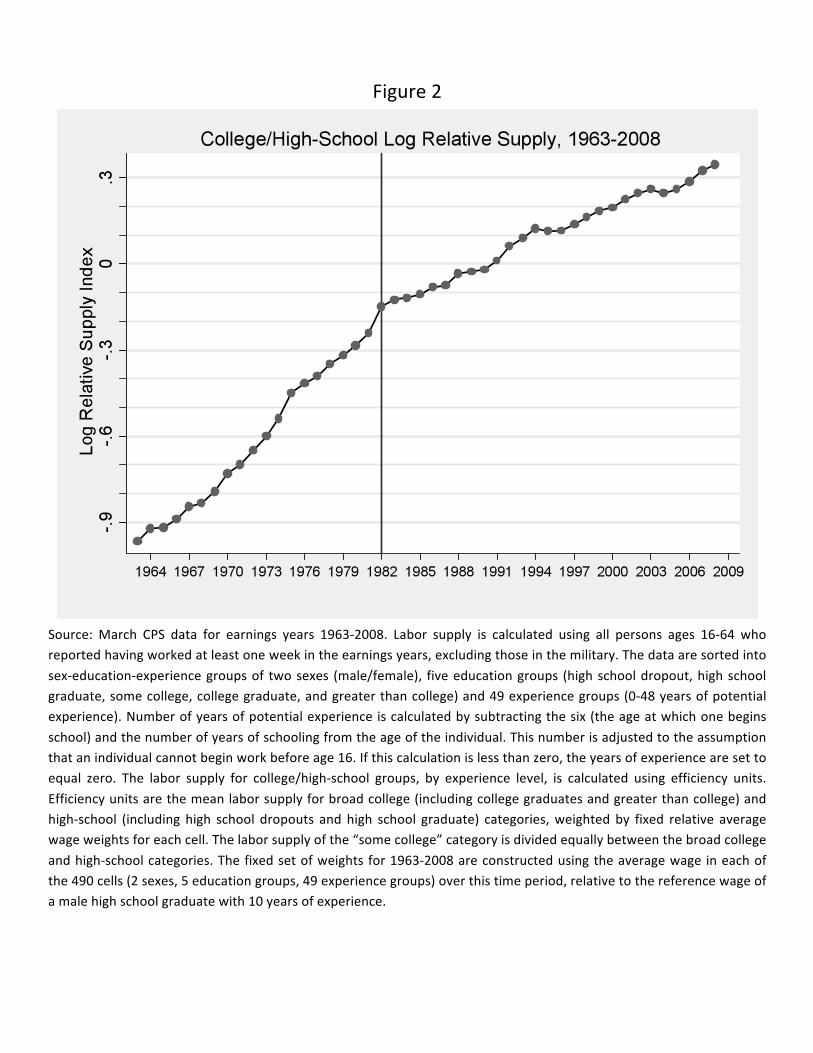
Figure  2  

 Source:   March   CPS   data   for   earnings   years   1963-­‐2008.   Labor   supply   is   calculated   using   all   persons   ages   16-­‐64   who  reported  having  worked  at  least  one  week  in  the  earnings  years,  excluding  those  in  the  military.  The  data  are  sorted  into  

sex-­‐education-­‐experience  groups  of   two  sexes   (male/female),   five  education  groups   (high  school  dropout,  high  school  graduate,  some  college,  college  graduate,  and  greater  than  college)  and  49  experience  groups  (0-­‐48  years  of  potential  experience).  Number  of  years  of  potential  experience  is  calculated  by  subtracting  the  six  (the  age  at  which  one  begins  

school)  and  the  number  of  years  of  schooling  from  the  age  of  the  individual.  This  number  is  adjusted  to  the  assumption  that  an  individual  cannot  begin  work  before  age  16.  If  this  calculation  is  less  than  zero,  the  years  of  experience  are  set  to  equal   zero.   The   labor   supply   for   college/high-­‐school   groups,   by   experience   level,   is   calculated   using   efficiency   units.  

Efficiency  units  are  the  mean  labor  supply  for  broad  college  (including  college  graduates  and  greater  than  college)  and  high-­‐school   (including   high   school   dropouts   and   high   school   graduate)   categories,  weighted   by   fixed   relative   average  wage  weights  for  each  cell.  The  labor  supply  of  the  “some  college”  category  is  divided  equally  between  the  broad  college  

and  high-­‐school  categories.  The  fixed  set  of  weights  for  1963-­‐2008  are  constructed  using  the  average  wage   in  each  of  the  490  cells  (2  sexes,  5  education  groups,  49  experience  groups)  over  this  time  period,  relative  to  the  reference  wage  of  a  male  high  school  graduate  with  10  years  of  experience.    

 

Figure  3a  

 Source:  March  CPS  data  for  earnings  years  1963-­‐2008.  See  note  to  Figure  2.  Log  relative  supply  for  0-­‐9  and  20-­‐29  years  

of  potential  experience  is  plotted  for  males  and  females.  

 

Figure  3b  

 

Figure  4a  

 Source:  March  CPS  data  for  earnings  years  1963-­‐2008.  See  note  to  Figure  1.  The  real  log  weekly  wage  for  each  education  

group   is   the   weighted   average   of   the   relevant   composition   adjusted   cells   using   a   fixed   set   of   weights   equal   to   the  average  employment  share  of  each  group.    

 

Figure  4b  

   

Figure  5a    

 Source:  May/ORG  CPS  data  for  earnings  years  1973-­‐2009.  For  each  year,  log  hourly  wages  for  all  workers,  excluding  the  self-­‐employed   and   those   employed   by   the   military,   are   regressed   on   a   quadratic   in   education   (eight   categories),   a  quartic  in  experience,  a  female  dummy,  and  interactions  of  the  female  dummy  and  the  quartic  in  experience.  Predicted  

real  log  hourly  wages  are  computed  in  1973,  1989  and  2009  for  each  of  the  years  of  schooling  presented  in  the  figure.  See  Data  Appendix  for  more  details  on  treatment  of  May/ORG  CPS  data.  

 

Figure  5b  

 

Figure  6a    

 Source:  May/ORG  CPS  data  for  earnings  years  1973-­‐2009.  For  each  year,  log  hourly  wages  for  all  workers,  excluding  the  self-­‐employed  and  those  employed  by  the  military,  are  regressed  on  eight  education  dummies,  a  quartic  in  experience,  a  

female  dummy,  and   interactions  of   the  female  dummy  and  the  quartic   in  experience.  Predicted  real   log  hourly  wages  are  computed  in  1973,  1989  and  2009  for  each  of  the  years  of  schooling  presented.  See  Data  Appendix  for  more  details  on  treatment  of  May/ORG  CPS  data.  

 

Figure  6b    

 

Figure  7a  

 Source:  March  CPS  data  for  earnings  years  1963-­‐2008.  For  each  year,  the  10th,  median  and  90th  percentiles  of  log  weekly  

wages  are  calculated  for  full-­‐time,  full-­‐year  workers.    

 

Figure  7b  

 

Figure  7c  

 

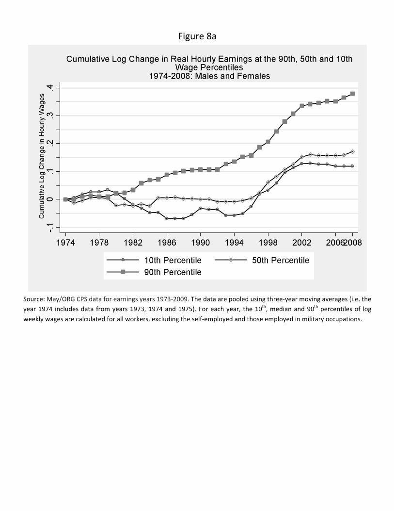
   Figure  8a  

 Source:  May/ORG  CPS  data  for  earnings  years  1973-­‐2009.  The  data  are  pooled  using  three-­‐year  moving  averages  (i.e.  the  year  1974   includes  data   from  years  1973,  1974  and  1975).  For  each  year,   the  10th,  median  and  90th  percentiles  of   log  

weekly  wages  are  calculated  for  all  workers,  excluding  the  self-­‐employed  and  those  employed  in  military  occupations.    

 

Figure  8b  

 

Figure  8c  

 

Figure  9a  

 Source:  May/ORG  CPS  data  for  earnings  years  1973-­‐2009.  The  data  are  pooled  using  three-­‐year  moving  averages  (i.e.  the  year  1974  includes  data  from  years  1973,  1974  and  1975).  For  each  denoted  time  period,  the  change  in  the  5th-­‐95th  

percentile  of  log  weekly  wages  is  calculated.

 

Figure  9b  

 

Figure  9c  

 

Figure  10  

 Source:  Census  IPUMS  5  percent  samples  for  years  1980,  1990,  and  2000,  and  Census  American  Community  Survey  for  2008.   All   occupation   and   earnings  measures   in   these   samples   refer   to   prior   year’s   employment.   The   figure   plots   log  changes  in  employment  shares  by  1980  occupational  skill  percentile  rank  using  a  locally  weighted  smoothing  regression  (bandwidth  0.8  with  100  observations),  where   skill   percentiles   are  measured  as   the  employment-­‐weighted  percentile  rank  of  an  occupation’s  mean  log  wage  in  the  Census  IPUMS  1980  5  percent  extract.  Mean  education  in  each  occupation  is   calculated   using  workers’   hours   of   annual   labor   supply   times   the   Census   sampling  weights.   Consistent   occupation  codes  for  Census  years  1980,  1990,  and  2000,  and  2008  are  from  Autor  and  Dorn  (2009a).  

Figure  11  

 Source:  Data  on  EU  employment  are  from  from  Goos,  Manning  and  Salomons,  2009a.  US  data  are  from  the  May/ORG  

CPS  files  for  earnings  years  1993-­‐2006.  The  data  include  all  persons  ages  16-­‐64  who  reported  having  worked  last  year,  excluding   those   employed   by   the  military   and   in   agricultural   occupations.  Occupations   are   first   converted   from   their  respective   scheme   into   326   occupation   groups   consistent   over   the   given   time   period.   These   occupations   are   then  

grouped  into  three  broad  categories  by  wage  level.    

Figure  12  

 Source:  May/ORG  CPS  files  for  earnings  years  1979-­‐2009.  The  data  include  all  persons  ages  16-­‐64  who  reported  having  worked   last   year,   excluding   those   employed   by   the   military   and   in   agricultural   occupations.   Occupations   are   first  

converted   from   their   respective   scheme   into   326   occupation   groups   consistent   over   the   given   time   period.   All   non-­‐military,  non-­‐agriculture  occupations  are  assigned  to  one  of  ten  broad  occupations  presented  in  the  figure.    

 Figure  13a  

 Source:  Census  IPUMS  5  percent  samples  for  years  1960,  1970,  1980,  1990,  and  2000,  and  Census  American  Community  Survey   for   2008.   The   data   include   all   persons   ages   16-­‐64   who   reported   having   worked   last   year,   excluding   those  

employed  by  the  military  and  in  agricultural  occupations.  Occupations  are  first  converted  from  their  respective  scheme  into   326   occupation   groups   consistent   over   the   given   time   period.   All   non-­‐military,   non-­‐agriculture   occupations   are  assigned  to  one  of  four  broad  occupations.    

 

 

Figure  13b  

 

Figure  13c  

 

Figure  14a  

 Source:  Census  IPUMS  5  percent  samples  for  years  1960,  1970,  1980,  1990,  and  2000,  and  Census  American  Community  Survey  for  2008.  See  note  to  Figure  15.  The  data  are  divided  into  four  educational  categories:  high  school  dropouts,  high  

school   graduates,   some   college   education,   and   college   graduates   or  more.   The   employment   share   of   the   four   broad  occupations  in  each  education  group  is  calculated  for  each  year,  and  the  cumulative  change  since  1959  is  plotted.  

 Figure  14b  

 

   

Figure  15  

 Source:  US  data   from  May/ORG  CPS  data   for  earnings  years  1992-­‐2009.  The  data   include  all  persons  ages  16-­‐64  who  reported  having  worked  last  year,  excluding  those  employed  by  the  military  and  in  agricultural  occupations.  Occupations  are  first  converted  from  their  respective  scheme  into  326  occupation  groups  consistent  over  the  given  time  period.  From  

these  groups,  occupations  are  then  consolidated  into  the  eight  broad  categories  presented  in  the  figure.  The  occupation  share  is  the  percentage  of  all  workers  employed  in  that  occupation.    

European  data  from  Eurostat  data  1992-­‐2008.  The  data  include  all  persons  ages  15-­‐59  who  reported  having  worked  in  the  last  year,  excluding  family  workers,  those  employed  by  the  military  and  in  agricultural  occupations.  Occupations  are  

grouped   into   the   eight   broad   categories   presented   in   the   figure.  Occupation   shares   are   calculated   using   unweighted  employment   data   for   ten   European   countries:   Denmark,   France,   Germany,   Greece,   Ireland,   Italy,   the   Netherlands,  Portugal,  Spain,  and  the  United  Kingdom.    

 

 Figure  16a  

 Source:  European  data  from  Eurostat  data  1992-­‐2008.  See  note  to  Figure  15.  Employment  shares  are  calculated  for  each  of  the  ten  European  countries  individually,  for  workers  under  40  years  of  age.  

   Figure  16b  

   

Figure  17a  

 Source:  Census  IPUMS  5  percent  samples  for  years  1960,  1970,  1980,  1990,  and  2000,  and  Census  American  Community  Survey  for  2008.  The  data   include  all   full-­‐time,  full-­‐year  workers  ages  16-­‐64,  excluding  those  employed  by  the  military  and  in  agricultural  occupations.    

Linear  education   consists  of   years  of   educational   attainment.   For   those  who  have  not   completed   second  grade,   their  years  of  education  are  imputed  based  on  gender  and  ethnicity.  For  those  who  have  completed  an  eighth  year  of  college  or  more,  their  years  of  education  are  imputed  with  20.5  years.  Education  dummies  consist  of  five  broad  categories:  high  school  dropouts,  high  school  graduates,  some  college  education,  college  graduates,  and  post-­‐college  degree.    

Occupations  are  first  converted  from  their  respective  scheme  into  326  occupation  groups  consistent  over  the  given  time  period.   From   these   groups,   occupations   are   then   consolidated   into   ten   broad   categories:   Managers;   Professionals;  Technicians;   Sales;   Office   and   administrative;   Production,   craft   and   repair;   Operators,   fabricators   and   laborers;  Protective  service;  Food  prep,  buildings  and  grounds,  cleaning;  and  Personal  care  and  personal  services.    

Industries  are  similarly  converted  from  their  respective  scheme  to  a  consistent  set  of  149  industries,  as  used  in  Autor,  Katz   and   Krueger   (1998).   From   these   149   industries,   ten   broad   industry   categories   are   constructed   and   include:  Construction;  Manufacturing;  Transport  and  utilities;  Wholesale  trade;  Retail  trade;  Finance,  Insurance  and  Real  Estate;  Business  services;  Personal  services  and  entertainment;  Professional  services;  and  Public  administration.    

The  partial  r-­‐squared  values  presented  above  are  equivalent  to  the  explanatory  power  of  the  respective  variable  group  in  log  weekly  wage  regressions.  Log  weekly  wages  and  each  variable  group  above  are  orthogonalized  using  a  quartic  in  experience  and  two  ethnicity  dummies.  Using  the  residuals  from  each  these  regressions,  residual  log  weekly  wages  are  regressed  separately  on  the  residuals  from  the  variable  groups  of  interest,  and  the  r-­‐squared  value  from  this  regression  is  plotted  above  for  each  year.  All  regressions  are  weighted  by  Census  person  weights.    

 

Figure  17b  

 

Figure  18a  

 Source:  Census  IPUMS  5  percent  samples  for  years  1960,  1970,  1980,  1990,  and  2000,  and  Census  American  Community  Survey  for  2008.  See  note  to  Figure  19  for  the  partial  r-­‐squared  calculation  procedure.  Five  O*Net  constructed  task  measures,  constructed  from  a  combination  of  O*Net  activities  and  context  scores,  are  utilized:  routine  cognitive,  routine  manual,  non-­‐routine  cognitive  analytic,  non-­‐routine  manual,  and  non-­‐routine  interpersonal.  Three  DOT  task  measures  are  utilized,  as  in  Autor,  Levy,  Murnane  (2003):  abstract,  routine,  and  manual.  See  the  Data  Appendix  for  more  information  on  the  construction  of  the  O*Net  task  measures.    

 

Figure  18b  

 

 

Figure  19  

 Source:  March  CPS  data  for  earnings  years  1963-­‐2008.  Log  weekly  wages  for  full-­‐time,  full-­‐year  workers  are  regressed  in  

each   year   on   four   education   dummies   (high   school   dropout,   some   college,   college   graduate,   greater   than   college),   a  quartic   in  experience,   interactions  of   the  education  dummies  and  experience  quartic,   and   two   race   categories   (black,  non-­‐white   other).   The   composition-­‐adjusted   mean   log   wage   is   the   predicted   log   wage   evaluated   for   whites   at   the  

relevant   experience   level   (5,   15,   25,   35,   45   years)   and   relevant   education   level   (high   school   dropout,   high   school  graduate,  some  college,  college  graduate,  greater  than  college).  The  mean   log  wage  for  college  and  high  school   is   the  weighted   average   of   the   relevant   composition   adjusted   cells   using   a   fixed   set   of   weights   equal   to   the   average  

employment  share  of  each  group.  The  ratio  of  mean   log  wages   for  college  and  high  school  graduates   for  each  year   is  plotted.  See  Data  Appendix  for  more  details  on  treatment  of  March  CPS  data.  The  Katz-­‐Murphy  predicted  wage  gap  are  

the  predicted  values  from  a  regression  of  the  college/high-­‐school  wage  gap  on  time  trend  term  and  log  labor  supply,  as  measured  in  efficiency  units  described  in  the  note  to  Figure  2,  for  years  1963-­‐1987.      

 

Figure  20  

 Source:  March  CPS  data  for  earnings  years  1963-­‐2008.  See  note  to  Figure  21.  The  detrended  supply  and  wage  series  are  the  residuals  from  separate  OLS  regressions  of  the  relative  supply  and  relative  wage  measures  on  a  constant  and  a  linear  time  trend.    

Figure  21a  

 Source:  March  CPS  data  for  earnings  years  1963-­‐2008.  See  note  to  Figure  22.  Log  college/high-­‐school  weekly  wage  ratio  for  0-­‐9  and  20-­‐29  years  of  potential  experience  is  plotted  for  males  and  females.  

 

Figure  21b