skills, schools and credit constraints: evidence … schools and credit constraints: evidence from...

Skills, Schools and Credit Constraints:Evidence from Massachusetts ∗

Joshua GoodmanEconomics Department, Columbia University

Mail: 1022 International Affairs Building420 W. 118th St., New York, NY 10027, USA

E-mail: [email protected]: 1-917-439-7907Fax: 1-212-851-2206

JEL Codes: I20, I22, I28Keywords: Credit constraints, academic skill, school districts, college enrollment

Abstract

Low college enrollment rates among low income students may stem from creditconstraints, low academic skill, low quality schools, or some combination of these.Recent Massachusetts data allow the first use of school district fixed effects in the anal-ysis of credit constraints, leading to four primary findings. First, Massachusetts’ lowincome students have lower intended college enrollment rates than higher incomestudents but also have dramatically lower skills and attend lower quality school dis-tricts. Second, inclusion of skill controls greatly reduces but does not eliminate the in-tended enrollment gap, with low income students seven percentage points less likelyto intend enrollment than similarly skilled higher income students. Third, in dis-tricts where higher income students are plausibly unconstrained, inclusion of schooldistrict fixed effects does little to reduce intended enrollment gaps, with low incomestudents nine percentage points less likely to intend enrollment than similarly skilledhigher income students from the same school district. Fourth, low income students inthe middle and upper parts of the skill distribution appear the most constrained, par-ticularly with respect to four-year public colleges. State governments could use themethods employed here to identify credit constrained student populations in order totarget financial aid more efficiently.

∗For their helpful comments, I thank Janet Currie, David Figlio, Sara Goldrick-Rab, Johannes Schmieder,Miguel Urquiola, and two anonymous referees, as well as participants of Columbia’s Applied Microeco-nomics Colloquium and the 2008 Annual Meeting of the Population Association of America.

1 Introduction and Previous Literature

In the U.S. and other developed countries, rapidly increasing college costs have raised

concerns about access to postsecondary education, particularly for low income students.

These concerns are heightened by the perceived need to improve the low-skilled segment

of the labor force in order to combat downward wage pressures attributed to globalization

and skill-biased technological change. In the U.S., advocates of increased financial aid

for postsecondary education are particularly concerned that students from low income

families enroll in college at significantly lower rates than do higher income students. As

of 2004, 49.6% of students from families in the lowest income quartile enrolled in college

immediately after high school graduation, compared to 79.3% of students from families

in the highest income quartile, a gap of nearly 30 percentage points.1

There are (at least) three potential explanations for this fact. The first is that low in-

come students have similar or higher returns to college education than do higher income

students but are financially constrained and thus can not afford further education. The

second is that low income students have lower academic skill and thus lower returns to

college education, so that their non-enrollment represents a rational, unconstrained de-

cision.2 The third, and until now relatively unexplored, explanation is that low income

students generally attend lower quality high schools than do higher income students, as

measured by the academic skills of the student populations, the expectations that stu-

dents enroll in college, and the resources devoted to factors that help students navigate

the college entrance process, such as guidance departments and standardized test prepa-

ration.

These three explanations are unfortunately easy to conflate given the high correlation

1These figures come from the 2004 October Supplement to the Current Population Survey.2Throughout this paper, I use “skill” to denote academic achievement as measured during high school

and take no position on the determinants of such achievement. What matters for the results below is thatskill defined in this way is a powerful predictor of college enrollment.

between family income, academic skill, and school quality. The inability to distinguish

these explanations creates a public policy quandary because each yields a different pol-

icy prescription. If low income students are financially constrained, public subsidies to

reduce college costs may improve the efficiency of human capital markets, an argument

for increasing financial aid. If low academic skills or school quality explain enrollment

gaps, then increasing financial aid may be ineffective or inefficient and public funds may

be better used trying to raise academic skills or improve school quality.

Attempts to distinguish these explanations are often frustrated by data limitations.

Most data sets, for example, lack any measure of academic skill, so that many authors

are forced to make indirect arguments about the existence of credit constraints.3 Thus,

supporting the importance of credit constraints are findings that college enrollment rates

are highly sensitive to financial aid (Kane, 1994; Dynarski, 2002) and to current income

(Mazumder, 2003), and that the existence of constrained students may explain why in-

strumental variables estimates of returns to schooling exceed ordinary least squares esti-

mates (Card, 1999). Indirect arguments against the importance of credit constraints come

from findings that the cyclicality of college enrollment does not differ by familial access to

credit (Christian, 2007) and that theoretical predictions about the reactions of credit con-

strained students to the opportunity and direct costs of college do not generate empirical

support for the existence of such students, at least in significant numbers (Cameron and

Taber, 2004).

Because the aforementioned papers lack measures of skill, it is hard to know exactly

how to interpret their results. More satisfying in this regard are papers that exploit the Na-

tional Longitudinal Surveys of Youth (NLSY), which contain such a measure in the form

3I focus here on credit constraints and the college enrollment margin. For recent work on whether creditconstraints affect the college completion decision, see Stinebrickner and Stinebrickner (2007), which arguesthat even generous policies to relieve credit constraints would have little impact on dropout rates. Forevidence after college graduation, see Rothstein and Rouse (2007), which argues that student reactions todebt are suggestive of the existence of credit constraints.

of the Armed Forces Qualification Test (AFQT) score. Using the 1979 NLSY, Cameron

and Heckman (2001) show that white-minority gaps in schooling attainment disappear

or even reverse sign when controlling for AFQT score. Similarly, Carneiro and Heckman

(2002) group students by skill and income to show small gaps by income once ability is

held constant. Their estimates suggest that skill and not income is the greatest constraint

to college enrollment.

Using similar methods, research by Ellwood and Kane (2000) and Belley and Lochner

(2007) suggests that credit constraints have become more important in recent years. Us-

ing the 1992 National Educational Longitudinal Study (NELS), which contains test scores,

Ellwood and Kane find that, conditional on ability, students in the lowest income quar-

tile are about 10 percentage points less likely to enroll in college than their higher in-

come peers. They also find that the importance of income as a predictor of enrollment

increased between the early 1980s and the early 1990s. Similarly, Belley and Lochner

replicate Carneiro and Heckman’s work using both the 1979 and the 1997 NLSY cohorts

and find that family income plays a much larger role in the determination of college en-

rollment for the younger cohort than for the older cohort. In a subsequent paper, Lochner

and Monge-Naranjo (2008) argue that this fact and the increasing demand by college en-

rollees for both public and private credit are consistent with increasingly binding credit

constraints, particularly on the lowest skilled students. In particular, the authors suggest

that these increased constraints stem from the rising costs of college coupled with the

relatively stable level of government financial aid available.

This paper uses an approach similar to the papers mentioned in the previous two para-

graphs, comparing low income students to higher income students of similar academic

skill, the latter of which are presumed to be an unconstrained control group. Instead of

the NLSY or NELS, this paper uses data on the college intentions, test scores and school

districts of all 2003 and 2004 Massachusetts public high school graduates.4 Though the

data set has limitations that will be discussed below, it offers two advantages over the

other data sets. First, it contains the universe of very recent public high school gradu-

ates from Massachusetts, allowing for a detailed description and precise estimates of one

state’s college market. Second and more important, it allows for the first use of school

district fixed effects in the analysis of credit constraints, making estimates of credit con-

straints even more convincing by comparing students who have different incomes but

attend the same school district.

There are four primary findings. First, Massachusetts’ low income students have

lower intended college enrollment rates than higher income students but also have dra-

matically lower academic skills and attend lower quality school districts. Second, in-

clusion of skill controls greatly reduces but does not eliminate the intended enrollment

gap, with low income students seven percentage points less likely to intend enrollment

in college than higher income students of the same skill. Third, in districts where higher

income students are a plausibly unconstrained control group, inclusion of school district

fixed effects does little to reduce intended enrollment gaps, with low income students

nine percentage points less likely to intend enrollment in college than higher income stu-

dents of the same skill and from the same school district. Fourth, low income students in

the middle and upper parts of the skill distribution appear the most constrained, particu-

larly with respect to four-year public colleges. State governments could use the methods

employed here to identify credit constrained segments of their student populations in

order to target financial aid more efficiently.

The paper proceeds as follows. Section 2 describes the data, including simple analysis

4The data also contain the class of 2005 but I omit those students because of the introduction of a meritscholarship program that based college aid directly on the test score employed here as a control. As Good-man (2008) shows, this aid had significant impacts on students’ enrollment decisions and might thus biasthe results.

of the relation between academic skill, low income status and intended college enroll-

ment. Section 3 employs a linear probability regression model to explore more rigorously

how the relation between low income status and intended college enrollment changes

when controlling for academic skill and school district. Section 4 concludes.

2 Data Description

The data come from Massachusetts’ Student Information Management System (SIMS)

and include every 2003 and 2004 public high school graduate, totalling over 100,000 stu-

dents. The most important variables contained in SIMS for each student are standardized

test scores, a low income indicator, a randomized school district identifier, and the stu-

dent’s post-graduation intentions as reported by her high school’s guidance department.

The data also contain each student’s gender, race, English as a second language status

and limited English proficiency status.

The standardized test scores come from the Massachusetts Comprehensive Assess-

ment System (MCAS), a math and English exam that all public school 10th graders must

take and eventually pass in order to graduate from high school. I sum students’ math

and English scores from their first sittings of the exam, transforming this score into both

a quartile and a Z-score by class in order to account for a slight year-to-year rise in test

scores. The randomized district identifier allows identification of students in the same

school district, as well as construction of measures such as each district’s low income

rate, median MCAS score, and graduating class size.5

The low income indicator is a measure of whether a student receives free or reduced

price school lunches.6 To receive such subsidies, the student must enroll in the school

5Because the district identifier is randomized, I can not merge this student-level data with external dataon the characteristics of the school districts.

6The data does not distinguish between free and reduced price lunch recipients.

lunch program, which she qualifies for if her family receives TANF or food stamps, or has

income below 185% of the federal poverty line. I refer to students receiving the subsidy

as “low income” and students not receiving it as “higher income”. In 2004, the federal

poverty line for a family of 4 was $18,850, so that here a low income student (from a family

of 4) has family income lower than $34,873 (=1.85*$18,850).7 For reference, according to

the 2004 American Community Survey, Massachusetts’ median family income was about

$55,600, though it was much lower for black families ($33,300) and Hispanic families

($36,300). Also, because this variable indicates only those who have chosen to enroll in the

lunch program, some of those labelled higher income in the data may be from low income

families that have not enrolled for whatever reason, which will cause underestimation of

the size of any credit constraints.

Students’ post-graduation intentions are reported as one of five categories: four-year

public college, four-year private college, two-year public college, two-year private col-

lege, or other (work, military, etc.). I use these categories to construct the more general

outcomes of intended enrollment in any college, any four-year college and any two-year

college.8 I also construct a measure of years of college in which each student initially

intends to enroll, a variable that takes on values 0, 2 and 4.

To check that students’ reported intentions reflect actual college enrollment, I use

IPEDS’ Residence and Migration data, which reports for each U.S. postsecondary insti-

tution the number of “first-time degree/certificate-seeking undergraduate students who

graduated from high school in the past 12 months,” broken down by students’ states

of residence at the time of admission to the institution. The proportions of students at-

tending various categories of college are nearly identical in the IPEDS and SIMS data.

According to IPEDS/SIMS, the proportions of these students attending four-year private

7Each additional family member adds $3,180 to the federal poverty line, which translates to an additional$5,883 (=1.85*$3,180) of family income added the low income threshold as defined here.

8The two-year category consists almost entirely of public community colleges.

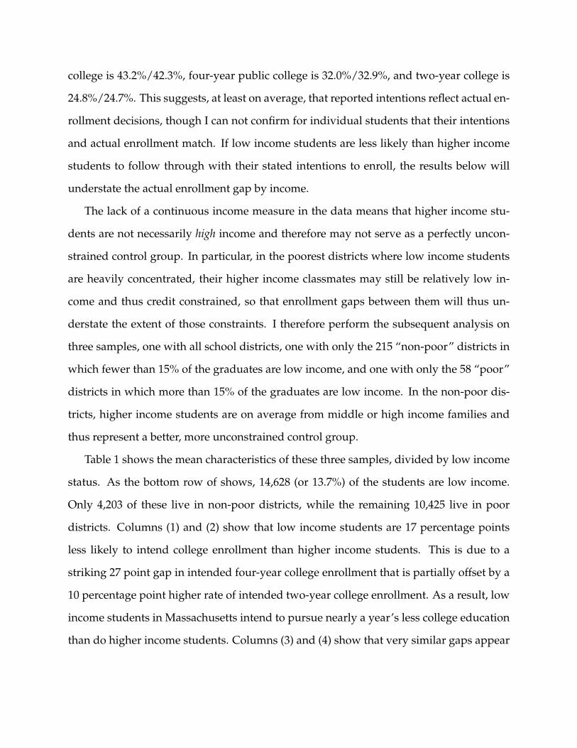
college is 43.2%/42.3%, four-year public college is 32.0%/32.9%, and two-year college is

24.8%/24.7%. This suggests, at least on average, that reported intentions reflect actual en-

rollment decisions, though I can not confirm for individual students that their intentions

and actual enrollment match. If low income students are less likely than higher income

students to follow through with their stated intentions to enroll, the results below will

understate the actual enrollment gap by income.

The lack of a continuous income measure in the data means that higher income stu-

dents are not necessarily high income and therefore may not serve as a perfectly uncon-

strained control group. In particular, in the poorest districts where low income students

are heavily concentrated, their higher income classmates may still be relatively low in-

come and thus credit constrained, so that enrollment gaps between them will thus un-

derstate the extent of those constraints. I therefore perform the subsequent analysis on

three samples, one with all school districts, one with only the 215 “non-poor” districts in

which fewer than 15% of the graduates are low income, and one with only the 58 “poor”

districts in which more than 15% of the graduates are low income. In the non-poor dis-

tricts, higher income students are on average from middle or high income families and

thus represent a better, more unconstrained control group.

Table 1 shows the mean characteristics of these three samples, divided by low income

status. As the bottom row of shows, 14,628 (or 13.7%) of the students are low income.

Only 4,203 of these live in non-poor districts, while the remaining 10,425 live in poor

districts. Columns (1) and (2) show that low income students are 17 percentage points

less likely to intend college enrollment than higher income students. This is due to a

striking 27 point gap in intended four-year college enrollment that is partially offset by a

10 percentage point higher rate of intended two-year college enrollment. As a result, low

income students in Massachusetts intend to pursue nearly a year’s less college education

than do higher income students. Columns (3) and (4) show that very similar gaps appear

between low and higher income students within the non-poor districts. Columns (5) and

(6) show gaps with the same signs but much smaller magnitudes in the poor districts.

None of this is necessarily evidence of credit constraints, given that the remainder of

Table 1 also shows that, compared to higher income students, low income students score

a full 0.8 standard deviations lower on the MCAS and are much more likely to graduate

from school districts that have lower median MCAS scores, lower incomes, and larger

graduating classes. As with the intended enrollment gaps, these gaps in characteristics

of students and their school districts persist within the set of non-poor districts and are

generally smaller in the poor districts.

To highlight the extraordinary disparity in academic skill between low income and

higher income students, panel (A) of Figure 1 shows the distribution of low income stu-

dents among the MCAS quartiles. If low income and academic skill were uncorrelated,

each quartile would contain 25% of low income students, as the dashed line shows. This

is not the case. A remarkable 53% of low income students score in the lowest quartile and

another 26% score in the second lowest quartile, whereas only 22% score in the top half

of the distribution. The results would be even more dramatic if the data included high

school dropouts, who are disproportionately low income and have low academic skills.

The remaining panels of Figure 1 give a simple sense of the extent to which low income

students’ low skills account for their low intended enrollment rates by plotting these rates

by MCAS quartile and low income status. Panel (B) shows that intended enrollment rates

and gaps vary by academic skill, with a low rate and nearly no gap for students in the

lowest quartile and higher rates and roughly 10 percentage point gaps for the upper three

quartiles. Panel (C) shows a similar pattern for the gap in intended enrollment in four

year colleges, though the gaps are slightly larger for the upper three quartiles than in

panel (A). This is offset by the fact, as shown in panel (D), that low income students in the

upper three quartiles are actually more likely to intend enrollment in two year colleges

than higher income students. In all three panels, the within-quartile gaps are smaller than

the overall gaps from Table 1. This suggests that a large part of the intended enrollment

gap can be explained by the fact that low-skilled students intend enrollment at relatively

low rates (regardless of income) and that low income students tend to have low skills.

Figures 2 and 3 replicate figure 1 with the sample divided into non-poor and poor

districts respectively. Comparing the two panels (A) from these figures shows that low

income students from non-poor districts have a less skewed skill distribution than do

low income students from poor districts, though well over two-thirds of the former still

fall into the bottom half of the distribution. Interestingly, though the intended enrollment

rates by quartile look roughly similar across the two sets of districts, the non-poor districts

show pronounced gaps while the poor districts show much smaller or non-existent gaps.

This may be due to the fact noted above that higher income students in non-poor districts

more closely resemble an unconstrained control group than do higher income students in

poor districts.

3 Regression Results

To quantify the intended enrollment gaps between low income and higher income stu-

dents more precisely, and to compare students within school districts, I use a linear prob-

ability model of the form

Collegeij =4∑

k=1

[αkQ

kij + βk

(LowIncij ×Qk

ij

)]+ γXij + Dj + εij (1)

where Collegeij indicates intended enrollment for student i in district j, LowIncij indi-

cates low income, Qkij is an indicator for the kth MCAS quartile, Xij is a vector of indi-

vidual controls (race, gender, English as a second language, limited English proficiency),

and Dj represent school district fixed effects. Given this specification, the coefficients βk

compare the enrollment decision of low income students to higher income students in the

same (kth) MCAS quartile and the same school district.9

The β’s are imperfect measures of credit constraint. As discussed above, they will

underestimate the extent of those constraints in districts where higher income students

do not come from high income, presumably unconstrained, families. Conversely, the β’s

may overestimate credit constraints if, even conditional on school district, they are cap-

turing low income families’ different tastes and information about college. Regardless of

these complications, coefficients derived from the above specification are a simple and

useful measure of credit constraint currently available to states for the purposes of finan-

cial aid policy. The question of interest to policymakers is whether giving a student aid

upon graduation from high school increases her probability of attending college. This aid

neither remedies skill gaps between students of various income levels nor does it com-

pensate for the differing qualities of the school districts students have attended. The β’s

therefore represent the best easily available estimate of the extent to which low income

students’ college enrollment patterns would change if they were provided with the same

access to credit for postsecondary education as higher income students have.

Table 2 shows the results of Equation 1, with each coefficient representing a sepa-

rate regression using various measures of intended enrollment as outcomes. Panel (A)

includes the full sample, with three specifications run on each outcome. The first spec-

ification omits skill and school district controls in order to get a “raw” measure of the

intended enrollment gap, the second specification includes skill controls, and the third

specification includes both skill controls and school district fixed effects.10 In panel (A),

9In the regressions that follow, none of the results change significantly if regressions are run separatelyby MCAS quartile or if probit specifications are used in place of linear probability models. I use linearprobability models for consistency given that the school district fixed effects specifications preclude the useof probits.

10Though not shown, the demographic controls in Table 2 are also interesting and may confirm that the

the raw gaps are quite similar to the mean differences seen in table 1, as expected. The

inclusion of skill controls more than halves all of these gaps, as figure 1 suggested would

be the case. The inclusion of school district fixed effects cuts these gaps roughly in half

again. Inclusion of school district fixed effects may be reducing the estimates of credit

constraints by controlling for the causal impact of school districts on intended enrollment

or by accentuating the comparison of low income students to their relatively low income

classmates.

To distinguish these possibilities, panels (B) and (C) separate the sample into non-poor

and poor districts respectively. A clear pattern now emerges. For non-poor districts, like

the full sample, inclusion of skill controls reduces intended enrollment gaps by half or

more. Inclusion of school district fixed effects has, however, relatively little further im-

pact, so that statistically and economically significant gaps remain between low income

students and their higher income classmates. In the poor districts, the raw intended en-

rollment gap is only five percentage points and, like in the upper two panels, is halved

by the inclusion of skill controls and then reduced only slightly by further inclusion of

school district fixed effects.11 That inclusion of school district fixed effects has little im-

pact in panels (B) and (C) suggests that their impact in panel (A) is not causal but instead

accentuates the poor districts where most low income students attend school and where

intended enrollment gaps are extremely small.

Three primary conclusions can be drawn from table 2. First, inclusion of skill controls

greatly reduces but does not eliminate the intended enrollment gap. Low income students

data are roughly accurate. For example, conditional on skill and school district, female students are morelikely to intend enrollment in every college category than male students, consistent with the increasinglydiscussed reverse gender gap in higher education. Similarly, black students are six percentage points morelikely to intend enrollment in four-year private colleges, which suggests either high returns to enrollmentor affirmative action. For recent evidence that black students have particularly high returns to college edu-cation due to its signalling value, see Arcidiacono, Bayer, and Hizmo (2008). For evidence that affirmativeaction for blacks is heavily concentrated in private four-year colleges, see Kane (1998).

11Running these regressions separately by gender yields nearly identical results for males and females.

are seven percentage points less likely to intend enrollment in any college and intend to

enroll in 0.3 fewer years of college than higher income students of the same skill. Sec-

ond, in non-poor districts where higher income students are a plausibly unconstrained

control group, inclusion of school district fixed effects has little impact on intended en-

rollment gaps, suggesting that school quality can not explain the gaps. In these districts,

low income students are nine percentage points less likely to intend enrollment in any

college and intend to enroll in 0.4 fewer years of college than higher income students of

the same skill and from the same school district. Third, in poor districts, intended enroll-

ment gaps conditional on skill and school district are extremely small, likely because the

higher income control group is itself relatively low income.

One question worth exploring is why, in panel (A) of table 2, the inclusion of school

district fixed effects greatly reduces estimates of the intended enrollment gap. To de-

termine what characteristics of school districts the fixed effects are picking up, table 3

replicates the first column of panel (A) where the outcome is intended enrollment in any

college. Columns (1) and (2) simply repeat panel (A)’s “skill controls” and “school district

fixed effects” specifications. Columns (3)-(7) omit the fixed effects and instead include

other district-level characteristics. Columns (3) and (4) show that inclusion of either the

district’s median MCAS score or the district’s low income rate has nearly the same im-

pact on the estimated gap as does inclusion of district fixed effects. Conversely, inclusion

of the fraction minority or the logarithm of the graduating class size in columns (5) and

(6) has little impact on the gap. This suggests that district-level academic skill and in-

come levels, not racial composition and size, are the most critical characteristics of school

districts affecting individual students’ intended enrollment. To see whether district-level

skill or income matters more, column (7) includes all four district-level controls, reveal-

ing that only the district’s median MCAS score retains any predictive power. Inclusion

of the other three controls barely changes the R2 when column (7) is compared to column

(3). As a whole, these results suggest that low income students’ distribution across school

districts of lower average achievement levels is the critical fact driving the results in panel

(A).

Finally, because figures 1, 2 and 3 suggest that intended enrollment gaps differ by

skill, table 4 replicates the bottom two panels of table 2 with the low income indicator

fully interacted with indicators for MCAS quartiles. In the non-poor districts, all four

quartiles show intended enrollment gaps. The largest gaps appear in the middle two

quartiles, due to a roughly 16 percentage point gap in intended four-year college enroll-

ment. Though low income students in all quartiles are less likely to intend enrollment

in four-year private colleges, only low income in the middle two quartiles are less likely

to intend enrollment in four-year public colleges. Such students do compensate by in-

tending to enroll in two-year colleges but the net result is that low income students in

the middle two quartiles intend to pursue 0.5-0.6 fewer years of education than do higher

income students of the same skill. Inclusion of school district fixed effects reduces these

gaps slightly but leaves the basic conclusions unchanged. In the poor school districts, it is

the upper two quartiles that exhibit the largest gaps, even after inclusion of school district

fixed effects. Again, gaps in intended four-year public college enrollment primarily drive

this result.

4 Conclusion

That inclusion of skill controls greatly reduces intended enrollment gaps is already a well-

established result. The persistence of such gaps within non-poor school districts is a new

finding that strengthens the argument for the existence of credit constraints, albeit for a

relatively small eight percent of the low income student population. These estimates are

remarkably similar to the roughly 10 percentage point gaps found by Ellwood and Kane

(2000) and Belley and Lochner (2007) between the lowest income quartile and the average

of the upper three quartiles.12 The lack of a continuous income measure does, however,

make it difficult to interpret the small gaps estimated in the poor school districts from

which most low income students graduate.

These numbers do suggest some good news for Massachusetts. Conditional on skill,

low income seems a relatively small constraint and more than 50% of the lowest skilled

graduates enroll in some form of college. This may be due to the fact that the state has

a highly-developed postsecondary market, with 30% more colleges per 15-19 year old

than the rest of the nation on average.13 Perhaps more importantly, it has college options

available at a wide range of price points. As of 2004, there were 15 community colleges

with an average annual tuition of $3,500, as well as 7 state colleges with an average annual

tuition of $5,400. The state spent an average of about $7,700 per full-time equivalent

student enrolled in public postsecondary institutions, the sixth highest of any state. That

credit constraints seem small is at least partially due to this extensive state support for

higher education. The overall enrollment gap would, for example, be larger if not for the

existence of inexpensive two-year community colleges, as seen in Table 4.

The bad news for Massachusetts lies in its student body’s skill distribution, where low

income is nearly a guarantee of low skill. The evidence presented here has three impli-

cations going forward. First, any further financial aid that Massachusetts plans should

target low income students with medium to high academic skills, possibly through four-

year public colleges, if the goal is to most efficiently raise postsecondary education levels.

Second, the state should consider devoting more of its budget to remedying the skill gap

present by the time low income students reach high school, a reallocation that might be

12See the third column of Table 10.4 in Ellwood and Kane (2000) and the last column of Table 3 in Belleyand Lochner (2007). Note that the estimates are not strictly comparable because those papers include highschool dropouts and measure actual attendance some time after high school graduation.

13This calculation is based on the number of colleges found in the Integrated Postsecondary EducationSystem and the number of 15-19 year olds calculated by the 2004 American Community Survey.

ultimately more effective at raising college enrollment rates than increased financial aid.

Third, given that all states now collect data on students’ academic skills, low income sta-

tus, and college enrollment, the methods employed in this paper could provide a useful

tool for each state to identify those sub-populations of students most likely to be finan-

cially constrained. This in turn might allow for the design of more effective, data-driven

financial aid programs.

REFERENCES

1. Arcidiacano, Peter, Patrick Bayer, and Aurel Hizmo, 2008. Beyond signaling andhuman capital: education and the revelation of ability. NBER Working Paper No.13951.

2. Belley, Philippe, and Lance J. Lochner, 2007. The changing role of family income andability in determining educational achievement. NBER Working Paper No. 13527.

3. Cameron, Stephen V., and James J. Heckman, 2001. The dynamics of educationalattainment for black, Hispanic, and white males. Journal of Political Economy 109:455-499.

4. Cameron, Stephen V., and Christopher Taber, 2004. Estimation of educational bor-rowing constraints using returns to schooling. Journal of Political Economy 112: 132-182.

5. Card, David, 1999. The causal effect of education on earnings. Handbook of LaborEconomics, Volume 3A, 1801-63. New York: Elsevier Science, North-Holland.

6. Carneiro, Pedro, and James J. Heckman, 2002. The evidence on credit constraints inpost-secondary schooling. Economic Journal 112: 705-734.

7. Christian, Michael S., 2007. Liquidity constraints and the cyclicality of college en-rollment in the United States. Oxford Economic Papers 59: 141-169.

8. Dynarski, Susan M., 2002. The behavioral and distributional implications of aid forcollege. American Economic Review 92: 279-85.

9. Ellwood, David T. and Thomas J. Kane, 2000. Who is getting a college education?Family background and the growing gaps in enrollment. In Securing the Future: In-vesting in Children from Birth to College, edited by Sheldon Danziger and Jane Wald-fogel. New York: The Russell Sage Foundation, pp. 283-324.

10. Goodman, Joshua S., 2008. Who merits financial aid? Massachusetts’ Adams Schol-arship. Journal of Public Economics, forthcoming.

11. Kane, Thomas J., 1994. College entry by blacks since 1970: the role of college costs,family background, and the returns to education. Journal of Political Economy 102:878-911.

12. Kane, Thomas J., 1998. Racial and ethnic preference in college admissions. InChristopher Jencks and Meredith Phillips (eds.), The Black-White Test Score Gap.Washington, DC: Brookings Institution Press.

13. Lochner, Lance J., and Alexander Monge-Naranjo, 2008. The nature of credit con-straints and human capital. NBER Working Paper No. 13912.

14. Mazumder, Bhashkar, 2003. Family resources and college enrollment. Federal Re-serve Bank of Chicago Economic Perspectives 27: 30-41.

15. Rothstein, Jesse, and Cecilia E. Rouse, 2007. Constrained after college: student loansand early career occupational choices. NBER Working Paper No. 13117.

16. Stinebrickner, Todd R., and Ralph Stinebrickner, 2007. The effect of credit con-straints on the college drop-out decision. NBER Working Paper No. 13340.

Figure 1: Skill Distribution and Intended Enrollment, All Districts

0.525

0.261

0.1460.069

0.1

.2.3

.4.5

.6%

of L

ow In

com

e St

uden

ts

1 2 3 4MCAS Quartile

(A) Distribution of Low Income Students

0.2

.4.6

.81

% In

tend

ing

Enro

llmen

t


(B) Any College

Higher incomeLow income

0.2

.4.6

.81

% In

tend

ing

Enro

llmen

t


(C) Four Year College


0.2

.4.6

.81

% In

tend

ing

Enro

llmen

t


(D) Two Year College


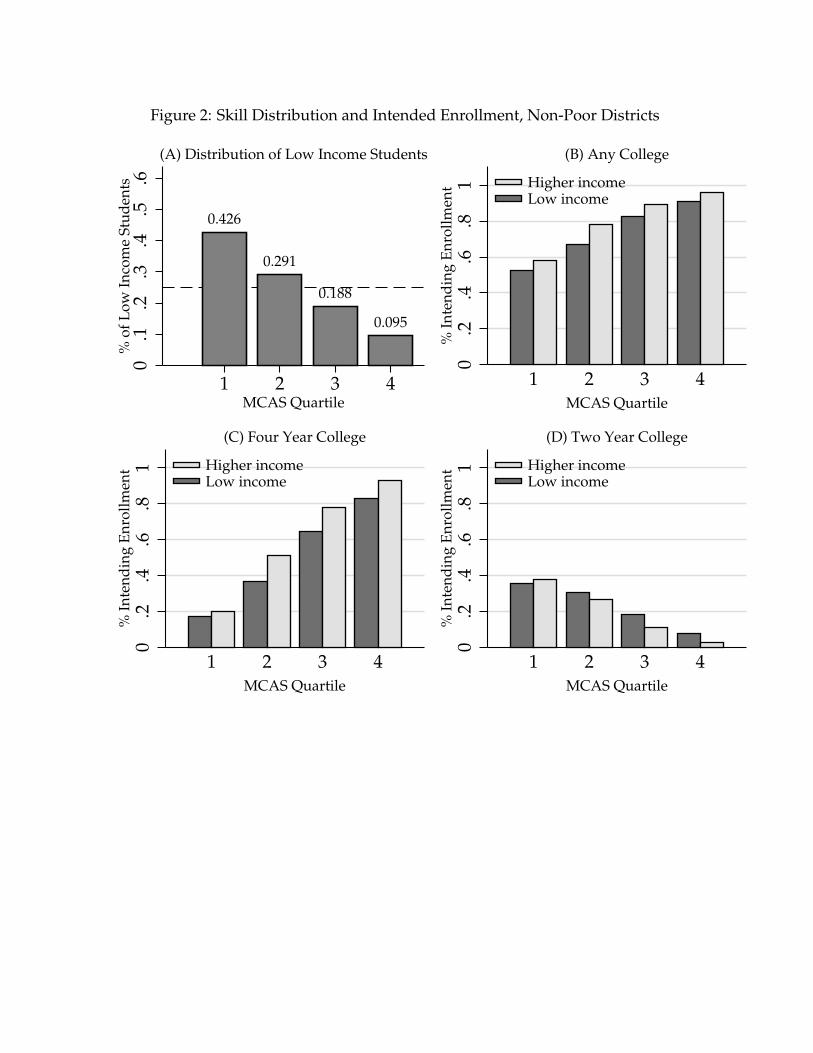
Figure 2: Skill Distribution and Intended Enrollment, Non-Poor Districts

0.426

0.291

0.188

0.095

0.1

.2.3

.4.5

.6%

of L

ow In

com

e St

uden

ts



0.2

.4.6

.81

% In

tend

ing

Enro

llmen

t


(B) Any College


0.2

.4.6

.81

% In

tend

ing

Enro

llmen

t




0.2

.4.6

.81

% In

tend

ing

Enro

llmen

t




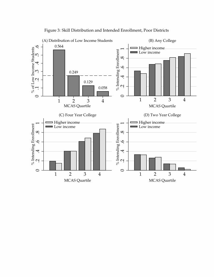
Figure 3: Skill Distribution and Intended Enrollment, Poor Districts

0.564

0.249

0.1290.058

0.1

.2.3

.4.5

.6%

of L

ow In

com

e St

uden

ts



0.2

.4.6

.81

% In

tend

ing

Enro

llmen

t


(B) Any College


0.2

.4.6

.81

% In

tend

ing

Enro

llmen

t




0.2

.4.6

.81

% In

tend

ing

Enro

llmen

t




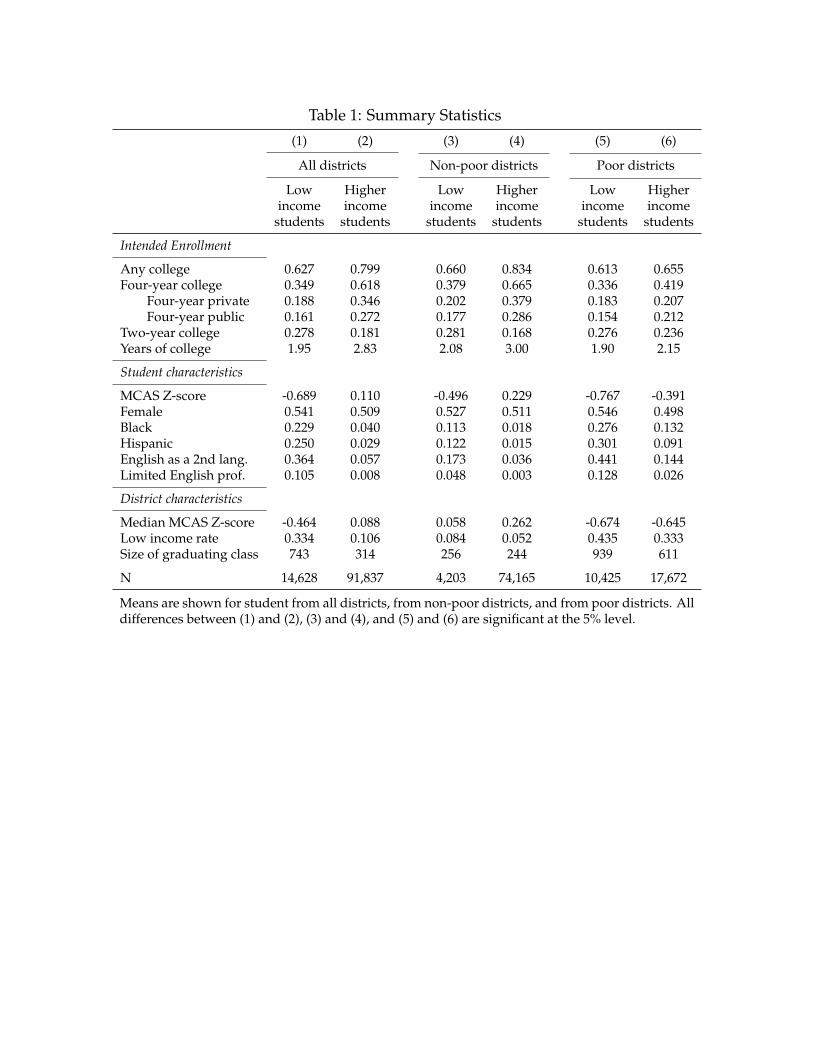
Table 1: Summary Statistics

(1) (2) (3) (4) (5) (6)

All districts Non-poor districts Poor districts

Low Higher Low Higher Low Higherincome income income income income income

students students students students students students

Intended Enrollment

Any college 0.627 0.799 0.660 0.834 0.613 0.655Four-year college 0.349 0.618 0.379 0.665 0.336 0.419

Four-year private 0.188 0.346 0.202 0.379 0.183 0.207Four-year public 0.161 0.272 0.177 0.286 0.154 0.212

Two-year college 0.278 0.181 0.281 0.168 0.276 0.236Years of college 1.95 2.83 2.08 3.00 1.90 2.15

Student characteristics

MCAS Z-score -0.689 0.110 -0.496 0.229 -0.767 -0.391Female 0.541 0.509 0.527 0.511 0.546 0.498Black 0.229 0.040 0.113 0.018 0.276 0.132Hispanic 0.250 0.029 0.122 0.015 0.301 0.091English as a 2nd lang. 0.364 0.057 0.173 0.036 0.441 0.144Limited English prof. 0.105 0.008 0.048 0.003 0.128 0.026

District characteristics

Median MCAS Z-score -0.464 0.088 0.058 0.262 -0.674 -0.645Low income rate 0.334 0.106 0.084 0.052 0.435 0.333Size of graduating class 743 314 256 244 939 611

N 14,628 91,837 4,203 74,165 10,425 17,672

Means are shown for student from all districts, from non-poor districts, and from poor districts. Alldifferences between (1) and (2), (3) and (4), and (5) and (6) are significant at the 5% level.

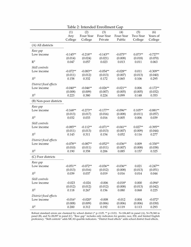
Table 2: Intended Enrollment Gap(1) (2) (3) (4) (5) (6)

Any Four-Year Four-Year Four-Year Two-Year Years ofCollege College Private Public College College

(A) All districts

Raw gapLow income -0.145** -0.218** -0.143** -0.075** 0.073** -0.727**

(0.014) (0.024) (0.021) (0.008) (0.018) (0.070)R2 0.047 0.057 0.023 0.013 0.011 0.063

Skill controlsLow income -0.072** -0.083** -0.054** -0.028** 0.011 -0.309**

(0.011) (0.012) (0.013) (0.007) (0.013) (0.040)R2 0.158 0.332 0.172 0.065 0.106 0.295

District fixed effectsLow income -0.040** -0.046** -0.026** -0.021** 0.006 -0.172**

(0.008) (0.009) (0.007) (0.005) (0.005) (0.032)R2 0.223 0.380 0.224 0.099 0.148 0.353

(B) Non-poor districts

Raw gapLow income -0.168** -0.273** -0.177** -0.096** 0.105** -0.881**

(0.013) (0.017) (0.016) (0.008) (0.011) (0.057)R2 0.032 0.033 0.016 0.005 0.006 0.039

Skill controlsLow income -0.085** -0.112** -0.071** -0.041** 0.027** -0.395**

(0.011) (0.013) (0.013) (0.007) (0.009) (0.044)R2 0.143 0.311 0.154 0.052 0.116 0.277

District fixed effectsLow income -0.078** -0.087** -0.052** -0.036** 0.009 -0.330**

(0.010) (0.011) (0.011) (0.007) (0.008) (0.038)R2 0.190 0.358 0.206 0.085 0.157 0.325

(C) Poor districts

Raw gapLow income -0.051** -0.072** -0.036** -0.036** 0.021 -0.247**

(0.013) (0.016) (0.012) (0.008) (0.013) (0.051)R2 0.039 0.037 0.019 0.016 0.014 0.044

Skill controlsLow income -0.023 -0.024 -0.006 -0.018* 0.000 -0.094*

(0.012) (0.012) (0.012) (0.008) (0.013) (0.042)R2 0.118 0.267 0.156 0.080 0.068 0.225

District fixed effectsLow income -0.016* -0.020* -0.008 -0.012 0.004 -0.072*

(0.008) (0.009) (0.006) (0.006) (0.006) (0.030)R2 0.200 0.312 0.192 0.119 0.113 0.293

Robust standard errors are clustered by school district (* p<0.05, ** p<0.01). N=106,465 in panel (A), N=78,368 inpanel (B), and N=28,097 in panel (C). “Raw gap” includes only indicators for gender, race, ESL and limited Englishproficiency. “Skill controls” adds MCAS quartile indicators. “District fixed effects” adds school district fixed effects.

Table 3: Other District-Level Controls and the Intended Enrollment Gap(1) (2) (3) (4) (5) (6) (7)

OLS FE —— Other district-level controls ——

Low income -0.072** -0.040** -0.041** -0.039** -0.058** -0.067** -0.038**(0.011) (0.008) (0.011) (0.008) (0.012) (0.012) (0.007)

District median MCAS score 0.111** 0.109**(0.017) (0.024)

District low income rate -0.270** -0.093(0.077) (0.211)

District fraction minority -0.142* 0.120(0.072) (0.136)

Ln(graduating class size) -0.019 -0.013(0.017) (0.014)

R2 0.158 0.223 0.175 0.165 0.160 0.159 0.176

Robust standard errors are clustered by school district (* p<0.05, ** p<0.01). N=106,465. Column (1) includes skill controls andindicators for gender, race, ESL and limited English proficiency. Column (2) adds school district fixed effects. The remainingcolumns omit the school district fixed effects. The outcome variable is intended enrollment in any college.

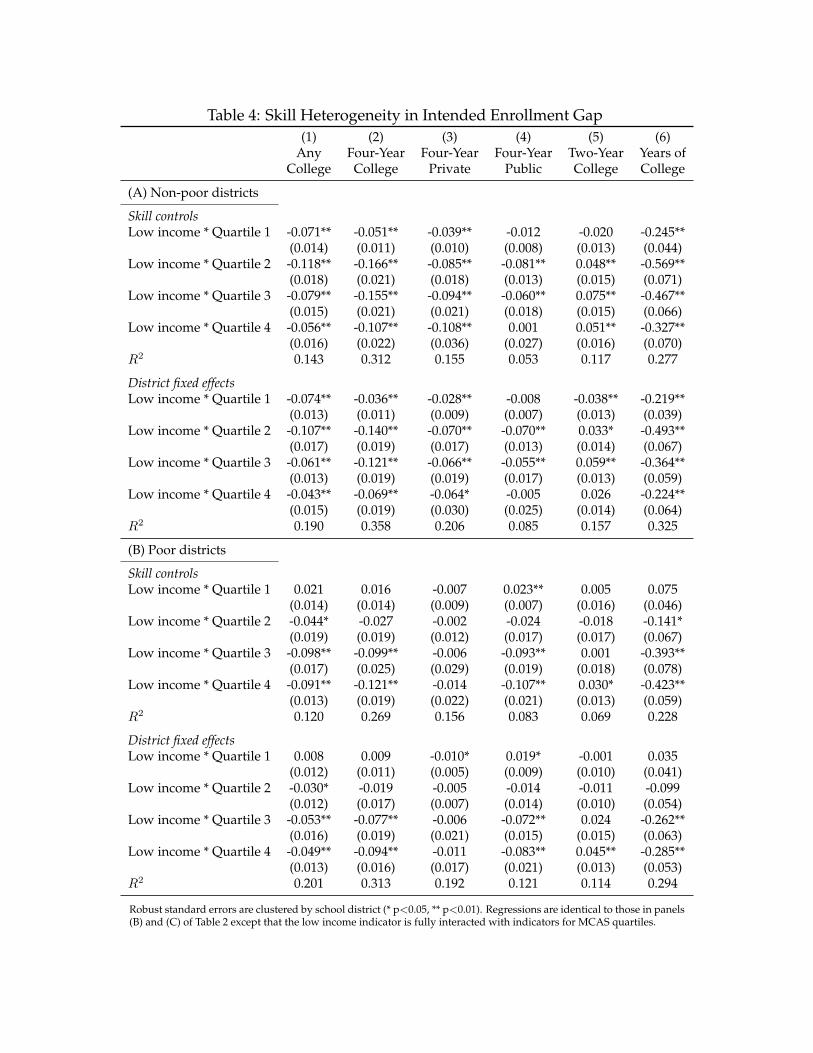
Table 4: Skill Heterogeneity in Intended Enrollment Gap(1) (2) (3) (4) (5) (6)

Any Four-Year Four-Year Four-Year Two-Year Years ofCollege College Private Public College College

(A) Non-poor districts

Skill controlsLow income * Quartile 1 -0.071** -0.051** -0.039** -0.012 -0.020 -0.245**

(0.014) (0.011) (0.010) (0.008) (0.013) (0.044)Low income * Quartile 2 -0.118** -0.166** -0.085** -0.081** 0.048** -0.569**


(0.015) (0.021) (0.021) (0.018) (0.015) (0.066)Low income * Quartile 4 -0.056** -0.107** -0.108** 0.001 0.051** -0.327**

(0.016) (0.022) (0.036) (0.027) (0.016) (0.070)R2 0.143 0.312 0.155 0.053 0.117 0.277

District fixed effectsLow income * Quartile 1 -0.074** -0.036** -0.028** -0.008 -0.038** -0.219**

(0.013) (0.011) (0.009) (0.007) (0.013) (0.039)Low income * Quartile 2 -0.107** -0.140** -0.070** -0.070** 0.033* -0.493**


(0.013) (0.019) (0.019) (0.017) (0.013) (0.059)Low income * Quartile 4 -0.043** -0.069** -0.064* -0.005 0.026 -0.224**

(0.015) (0.019) (0.030) (0.025) (0.014) (0.064)R2 0.190 0.358 0.206 0.085 0.157 0.325

(B) Poor districts

Skill controlsLow income * Quartile 1 0.021 0.016 -0.007 0.023** 0.005 0.075

(0.014) (0.014) (0.009) (0.007) (0.016) (0.046)Low income * Quartile 2 -0.044* -0.027 -0.002 -0.024 -0.018 -0.141*

(0.019) (0.019) (0.012) (0.017) (0.017) (0.067)Low income * Quartile 3 -0.098** -0.099** -0.006 -0.093** 0.001 -0.393**

(0.017) (0.025) (0.029) (0.019) (0.018) (0.078)Low income * Quartile 4 -0.091** -0.121** -0.014 -0.107** 0.030* -0.423**

(0.013) (0.019) (0.022) (0.021) (0.013) (0.059)R2 0.120 0.269 0.156 0.083 0.069 0.228

District fixed effectsLow income * Quartile 1 0.008 0.009 -0.010* 0.019* -0.001 0.035

(0.012) (0.011) (0.005) (0.009) (0.010) (0.041)Low income * Quartile 2 -0.030* -0.019 -0.005 -0.014 -0.011 -0.099

(0.012) (0.017) (0.007) (0.014) (0.010) (0.054)Low income * Quartile 3 -0.053** -0.077** -0.006 -0.072** 0.024 -0.262**

(0.016) (0.019) (0.021) (0.015) (0.015) (0.063)Low income * Quartile 4 -0.049** -0.094** -0.011 -0.083** 0.045** -0.285**

(0.013) (0.016) (0.017) (0.021) (0.013) (0.053)R2 0.201 0.313 0.192 0.121 0.114 0.294

Robust standard errors are clustered by school district (* p<0.05, ** p<0.01). Regressions are identical to those in panels(B) and (C) of Table 2 except that the low income indicator is fully interacted with indicators for MCAS quartiles.

skills, schools and credit constraints: evidence … schools and credit constraints: evidence from...

Documents