Credit Constraints, Equity Market Liberalization, andGrowth Rate Asymmetry�

Alexander Popovy

European Central Bank

Abstract

This paper provides evidence that �nancial openness is an important determinantof growth rate asymmetry in emerging markets. I exploit exogenous shocks to �nancial�ows and examine the impact of equity market liberalization on the skewness of out-put growth for 93 countries in the 1973-2009 period. I show that opening the economyto foreign portfolio investment results in a substantially higher negative skeweness ofoutput growth. This result is not driven by cross-country di¤erences in income, insti-tutional quality, domestic �nancial development, or trade. Moreover, it obtains withequal strength in the aggregate data and in the sectoral data, and it is dispropor-tionately stronger in sectors that require more external �nance. The increase in thenegative skewness of output growth after liberalization is mostly driven by an increasein the negative skewness of investment, TFP, and employment growth. The e¤ect islarger in countries that are more open to trade.JEL classi�cation: E32, F36, G15.Keywords: Financial openness, business cycle asymmetry, development.

�I thank Sandro Andrade, Geert Bekaert, Frederic Boissay, Markus Brunnermeier, Mario Crucini, SimonGilchrist, Pierre-Olivier Gourinchas, Francois Gourio, Wouter den Haan, Marie Hoerova, Jean Imbs, OlivierJeanne, Urban Jermann, Bartosz Mackowiak, Simone Manganelli, Kalina Manova, Steven Ongena, ValerieRamey, Romain Ranciere, Helene Rey, Jeremy Stein, Eric van Wincoop, Jaume Ventura, Francis Warnock,and seminar participants at the ECB, the 10th Darden International Finance Conference, the 2011 EFAConference, Stanford University, Boston University, and the 2011 Federal Reserve Bank of Chicago AnnualInternational Banking Conference for useful comments. The opinions expressed herein are those of the authorand do not necessarily re�ect those of the ECB or the Eurosystem.

yEuropean Central Bank, Financial Research Division, Kaiserstrasse 29, D-60311 Frankfurt, email:Alexander.Popov@ecb.int

1 Introduction

This paper presents evidence that credit constraints are an important determinant of growth

rate asymmetry in emerging markets. I exploit shocks to the availability of external �nance

and study the impact of equity market liberalization on the negative skewness of output

growth. Using a sample of 93 countries, I show that over the 1973-2009 period countries that

became �nancially open experienced a large increase in the negative skewness of GDP growth

relative to otherwise similar countries that remained closed to foreign portfolio investment.

Figure 1 illustrates the main result of the paper. It shows that over this period, the skewness

of GDP growth declined globally. However, while for the countries that did not liberalize

their stock markets, average GDP growth skewness declined from -0.0004 in 1991 (the median

liberalization year in the sample) to -0.1913 15 years later, for the countries that opened

their markets to foreign portfolio investment during the sample period, average GDP growth

skewness declined from -0.0930 in the liberalization year to -0.8513 15 years later.

This result is important in at least two ways. First, it is well-know that the behavior of

macroeconomic aggregates such as output and investment exhibits an asymmetric growth

pattern: booms are generally gradual and long-lasting, with growth rates not far from trend,

while downturns are generally sharp, with growth rates far below trend for a short period

of time (see Neftci, 1984; Hamilton, 1989; Diebold and Rudebusch, 1990; Morley and Piger,

2012). Most theoretical mechanisms proposed to explain this pattern rely on a learning

process in which either bad signals are more extreme than good signals, or signals are less

noisy during booms.1 This view, however, abstracts from market frictions that may arise

from agency problems, leading to an ampli�cation of fundamental shocks in the presence of

binding borrowing constraints. For example, credit frictions can amplify the e¤ects of credit

shocks on asset prices and these e¤ects can be transmitted across countries in a �nancially

integrated world (Caballero and Krishnamurthy, 2001; Gertler et al., 2007; Mendoza and

Quadrini, 2010). This mechanism implies that while growth rate asymmetry in itself may

1See Van Nieuwerburgh and Veldkamp (2006) for a thorough review.

1

be hardwired in the business cycle for reasons unrelated to properties of credit markets,

its evolution over time may be intimately related to changes in the availability of external

�nance. My paper is a �st empirical test of the empirical link between credit constraints

and business cycle asymmetry.

Second, since 1980 many emerging markets have lifted restrictions on cross-border �nan-

cial transactions. Consequently, economic research has focused intensely in recent years on

the e¤ect of �nancial openness on output growth rates. The evidence shows that �nancial

liberalization is associated, causally, with better prospects for future growth (e.g., Bekaert

et al., 2001, 2005; Quinn and Toyoda, 2008; Gupta and Yuan, 2009). However, while there is

strong evidence that shocks to trend growth are the primary source of �uctuations in emerg-

ing markets, as opposed to symmetric transitory �uctuations around the trend (Aguiar and

Gopinath, 2007), there has been no attempt to link empirically the process of �nancial

liberalization to growth rate asymmetry. My paper is a �rst attempt to bridge this gap.

While the central part of the paper relies on aggregate data, cross-country analysis is

prone to both conceptual and econometric problems. To address this issue, in the second

part of the paper I extend the analysis to the level of the industrial sector and exploit the

variation in the impact of increased availability of external �nance across sectors. Industries

that generate enough cash �ows to �nance investment should be less sensitive to changes in

access to external funds. Conversely, the availability of outside capital is crucial for sectors

which are highly dependent on external �nance for technological reasons (Rajan and Zingales,

1998). By exposing the economy to credit shocks originating abroad, �nancial globalization

should therefore disproportionately a¤ect growth rate asymmetry in �nancially vulnerable

sectors that require more external funds. Exploiting the cross sectional variation in external

�nancial dependence further helps establish a causal link from credit frictions to business

cycle asymmetry.

I �nd strong support for this prediction in a sub-sample of countries for which sectoral

data are available. I generate an interaction term of the indicator of �nancial liberalization

2

and the industry benchmark of �nancial vulnerability. As in Rajan and Zingales (1998), I use

each sector�s total capital expenditures minus cash �ow from operations, divided by capital

expenditures, for mature Compustat �rms, to de�ne external �nancial dependence. Using

this empirical strategy, I show that �nancial openness has a signi�cant negative e¤ect on

the skewness of sectoral value added growth over the same period as in the regressions using

aggregate data. Furthermore, this e¤ect is disproportionately stronger in sectors which rely

on external �nance for technological reasons. These results obtain with country, industry,

and time �xed e¤ects, which account for systematic di¤erences across countries and sectors

and capture general time trends.

I subject my main results to a battery of alternative tests. First and foremost, I address

the endogeneity of the liberalization decision. Countries tend to open their markets to

foreign portfolio investment at times of good growth opportunities (for example, before

joining and economic union such as the EU). Therefore, the treatment - �nancial openness

- is not randomly assigned. I account for this non-random choice by selecting best non-

liberalized matches for each liberalized country at each point in time. To that end, I use a

logistic regression to determine each country�s propensity score based on a number of country

characteristics, and then use the best matches as a control group in the regressions. Second,

I present robust results using measures of the comprehensiveness of liberalization. I also

address various data issues related to the number of sectors analyzed and to the choice of a

sample period. My main results remain remarkably robust to these alternative speci�cations.

Finally, I account for the fact that �nancial openness may be a part of a broader program

of development. While I �nd that wealthier economies and economies with deeper domestic

credit markets tend to have more asymmetric business cycles, the e¤ect of �nancial openness

on output skewness remains qualitatively unchanged.

The increase in the negative skewness of output growth is primarily realized through a

more negatively skewed distribution of investment, TFP, and employment growth. At the

same time, I �nd no e¤ect through the channel of new business creation. These results relate

3

to arguments about the channels through which �nancial liberalization-induced fragility

a¤ects real economic activity (Stiglitz, 2000). They also extend recent research evaluating

the welfare gain (loss) of �nancial openness (Gourinchas and Jeanne, 2006). Finally, the

negative e¤ect of equity market liberalization on growth rate asymmetry is larger in countries

that are more open to trade, suggesting that open countries may be exposed to the twin

risks of capital out�ows and terms of trade risk.

My paper contributes to a large literature on the e¤ect of �nancial openness on macroeco-

nomic volatility. Stiglitz (2000), Kose et al. (2006), and Levchenko et al. (2009) argue that

foreign capital increases volatility both in the �nancial markets and in the real economy.

Others (e.g., Easterly et al., 2001) �nd no e¤ect of �nancial openness on macroeconomic

volatility, or even a negative e¤ect on consumption volatility (Bekaert et al., 2006).2 My

contribution relative to the latter studies is to look at the e¤ect of �nancial openness on

the asymmetric (skewness) rather than the symmetric (variance) component of economic

�uctuations. In that sense, this paper is most closely related to Ranciere et al. (2008) who

study the link between �nancial liberalization, growth, and �nancial crises. In their model,

in a �nancially liberalized economy with limited contract enforcement, systemic risk taking

reduces the e¤ective cost of capital and relaxes borrowing constraints. This allows greater

investment and generates higher long-term growth, but it raises the probability of a sudden

collapse in �nancial intermediation when a crash occurs. Systemic risk thus increases mean

growth even if crises have arbitrarily large output and �nancial distress costs. While the

authors test empirically the link between long-term growth and �nancial fragility, proxied

by the skewness of credit growth, my paper presents the �rst direct test of the link between

�nancial openness and the skewness of output growth. This is a paper about the pattern of

economic �uctuations, not about �nancial crises.

In addition to being a description of business cycle asymmetry, output skewness is also

related to the concept of disaster risk. While much attention has been devoted in recent years

2For a comprehensive review of the literature on the volatility e¤ects of �nancial liberalization, see Koseet al. (2006) and Henry (2007), among others.

4

to the determinants of macroeconomic volatility - among them, credit market imperfections

- the welfare loss of higher business cycle volatility may ultimately be miniscule (Lucas,

1987). At the same time, it has recently been demonstrated that within a class of models

which replicate how asset markets price consumption uncertainty, individuals are willing

to pay a high premium in exchange for eliminating all chances for rare, large, and abrupt

macroeconomic contractions (Barro, 2006, 2009). To the extent that output risk cannot

be fully insured, the same increase in volatility would have considerably larger negative

implications for consumer welfare if it came from one single large contraction than if it came

from a series of symmetric deviations from a stable growth path.

My work is also related to a strand of literature which links �nancial openness to sudden

stops, capital �ights, and crises in emerging markets. One branch of this literature empha-

sizes the role of sovereign risk. In some of these models, strategic default - both on foreign

debt or on both foreign and domestic debt - can lead to large out�ows of capital, and that

e¤ect depends on the level of development as well as on the degree of debt enforcement

(see Eaton and Gersowitz, 1981; Atkeson, 1991; Aguiar and Gopinath, 2006; Aguiar et al.,

2009; Bai and Zhang, 2010; Broner and Ventura, 2010). Other work builds on �nancial

accelerators-type mechanisms to model international �nancial contagion. In these models,

credit constraints amplify the shocks that originate in one country and then spread to an-

other country (see Caballero and Krishnamurthy, 2001; Mendoza and Smith, 2006; Caballero

et al., 2008; Mendoza et al., 2009; Mendoza and Quadrini, 2010). In addition, various open

economy real business cycle theory models have proposed mechanisms for why opening the

country�s �nancial markets to foreign investment may increase the probability of a collapse

in domestic production following a sudden loss of access to international capital markets

(Mendoza, 1991; Calvo and Mendoza, 1996; Arellano and Mendoza, 2002). My paper can

be viewed as an empirical test of the latter models, with negative output skewness serving

as an empirical proxy for sharp and large contractions.

The paper proceeds as follows. Section 2 describes the data. Section 3 presents the

5

empirical methodology and reports the main results, alongside a battery of robustness tests.

Section 4 concludes.

2 Data

To examine the e¤ect of �nancial openness on output growth asymmetry I combine data on

equity market liberalization, output growth at the aggregate and sectoral level, and external

dependence by sector. I also employ a number of control variables. This section describes

the data I use.

2.1 Financial openness

The literature on �nancial openness uses various measures of de jure liberalization. Quinn

(1997), Bekaert et al. (2005), and Kaminsky and Schmukler (2008), among others, have

dated various liberalization events pertinent to capital accounts, credit markets, and equity

markets. In this paper, I use the Bekaert et al. (2005) classi�cation of equity market

liberalization events. In their dataset, liberalization events are available for 95 countries

starting in 1980. However, I extend the data back to 1973 using the Kaminsky and Schmukler

(2008) taxonomy of equity market liberalization events for countries which liberalized their

stock markets between 1973 and 1980 and so are treated as open by Bekaert et al. (2005).

In addition to the o¢ cial year of equity market reform, Bekaert et al. (2005) provide data

on the intensity of liberalization. This is a purely cross-sectional variable which captures the

ratio of International Finance Corporation (IFC) investable to global market capitalization.

It varies between 0 and 1 where a ratio of 1 implies no foreign ownership restrictions.

I use two main proxies for the e¤ect of �nancial openness on output growth rate asymme-

try. First, I construct a variable Liberalized, a dummy which equals 1 in the year of and all

years after an o¢ cial liberalization event. Second, I generate a variable Liberalization inten-

sity, an interaction between Liberalized (which varies across countries and over time) and the

6

IFC-related variable on foreign ownership restrictions (which only varies across countries).

This variable measures the proportion of domestic stocks that foreigners can invest in. Data

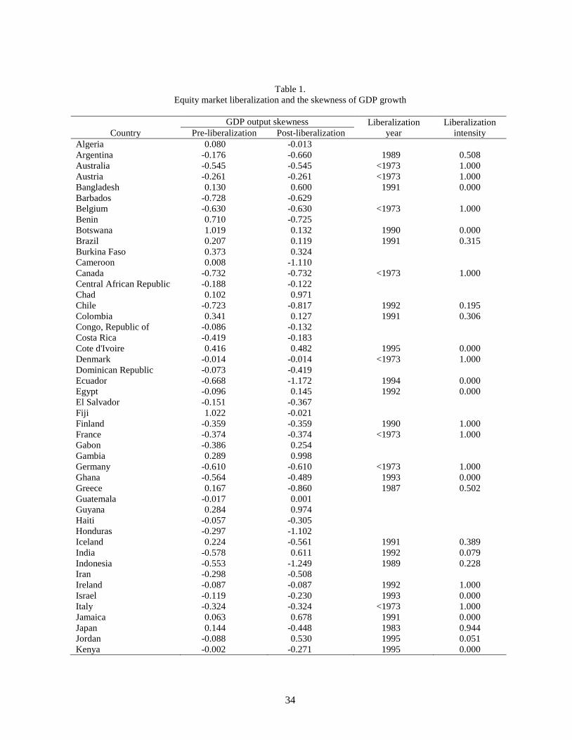
on both variables are summarized in Table 1.

2.2 Output growth

I obtain data on output growth from two sources. From the Penn World Tables, I obtain

data on real GDP growth rates (GRGDPCH) for the 95 countries in Bekaert et al. (2005)

for the period 1973-2009. I exclude Kuwait and Saudi Arabia for both of which data on

GDP growth only start in 1987. This results in a balanced panel of 93 countries. During

1973-2009, 46 countries opened to foreign equity �ows, while 13 liberalized prior to 1973,

and 34 never removed stock market restrictions (see Table 1).

Next, I obtain data on value added growth at the sector level from the 2010 UNIDO

Industrial Statistics 2 Database. I use the version that reports data according to the 2-digit

level of ISIC Revision 3 classi�cation. I restrict the sample period to 1973-2007 (2007 is the

last year with data). The dataset contains data on 21 manufacturing sectors, as well as on

total manufacturing.3 Similar to Levchenko et al. (2009), I use the data reported in current

U.S. dollars and convert them into international dollars using the Penn World Tables.4 I

require that each sector contains data on at least 30 years, to make the analysis comparable

to the one where GDP growth data are used. This results in the exclusion of a number of

countries with patchy data on value added growth for most or all industries. The resulting

dataset for the sector-level analysis consists of 37 countries relative to the 93 countries used

in the aggregate-level analysis.

Data on GDP growth skewness, both pre- and post-liberalization (for non-liberalized

countries, the cut-o¤ is set at the medium liberalization year for the sample, 1991), are

summarized in Table 1.3Data are not available for two additional industries, Motor vehicles, trailers, semi-trailers, and Recycling.4The exact mechanism is as follows. Using the variable name conventions from the Penn World Tables,

this de�ation procedure involves multiplying the nominal U.S. dollar value by (100 / P) * (RGDPL / CGDP)for output to obtain the de�ated value. See Levchenko et al. (2009) for more details.

7

2.3 External �nancial dependence

Rajan and Zingales (1998) argue that the distribution of growth rates would be most sensitive

to �nancial development in industries which are "naturally" dependent on external �nance.

Such "natural" dependence may arise due to variations in the scale of projects, gestation

period, the ratio of hard vs. soft information, the ratio of tangible vs. intangible assets,

follow-up investments, etc. In the sector-level analysis, I use the measure of external �nancial

dependence originally proposed by Rajan and Zingales (1998) for SIC 3-digit industries and

later adapted by Cetorelli and Strahan (2006) for SIC 2-digit industries. The benchmark is

de�ned as the industry median value of the sum across years of total capital expenditures

minus cash �ow from operations, divided by capital expenditures, for mature Compustat

�rms.5

The median of external �nance dependence across all 21 sectors is 0 and external de-

pendence ranges from -0.96 in industry "Leather and leather products" to 0.28 in industry

"Chemicals and allied products". In general, sectors with the greatest need for outside

capital tend to be intensive in large upfront investments, such as professional and scienti�c

equipment, electric machinery, and sectors engaged in the extraction of natural resources.

On the other hand, sectors engaged in the production of non-ferrous metals, apparel, and

foods and beverages are among the least external �nance dependent industries. Table 2

summarizes the sector-level data on external dependence.

2.4 Control variables

In addition, I employ a range of variables that control for other channels that may be

driving changes in growth rate asymmetry, both in the aggregate and in the sector-level

data. Countries with liberalized �nancial markets are usually more developed in a host

of other dimensions: they have higher income per capita, better institutions, and more

5The exact procedure involves subtracting from the sum across years of total capital expenditures (Com-pustat item #128) the cash �ow from operations, i.e., revenues minus nondepreciation costs (Compustatitem #110) for each �rm in Compustat, and then taking the median industry value as the benchmark.

8

developed domestic �nancial markets, are more open to trade, and have larger governments.

All of these parallel macroeconomic circumstances may be a¤ecting the skewness of output

growth. For example, trade openness may increase growth rate variability by exposing

the economy to terms of trade shocks (Rodrik, 1998); good institutions tend to mitigate

macroeconomic volatility (Acemoglu et al., 2003); out-of-trend credit growth may increase

the probability of crises (Kaminsly and Reinhart, 1999); a larger government sector may

stabilize the business cycle (Gali, 1994); and larger countries tend to have more diversi�ed

economies (Alesina and Wacziarg, 1998). In order to account for all these parallel factors, I

collect data on institutional quality from Polity IV, on domestic credit to private institutions

from Beck et al. (2010), and on per-capita income, government spending, population, and

trade openness from the World Penn Tables.

I also account for the fact that the impact of some of these factors will vary across

industries. For example, �nancial development and diversi�cation mechanisms should a¤ect

more strongly industries with naturally high liquidity needs (Raddatz, 2006). Analogously,

trade openness will matter less for non-tradeable sectors than for tradeable ones. To control

for these industry channels, I use Raddatz�s (2006) measure of liquidity needs6 and the ratio

of imports and exports to total output from Di Giovanni and Levchenko (2009). In both

cases, I aggregate 3-digit industry benchmarks to the SIC 2-digit level. Table 2 summarizes

these sector-level controls.

For de�nitions of all variables included in the paper, alongside variable sources, see Ap-

pendix 1.

3 Financial liberalization and growth rate asymmetry

I take two estimation approaches to establish the impact of �nancial liberalization on growth

rate asymmetry. First, I employ a panel analysis using aggregate data on GDP growth and6The exact procedure involves dividing the value of total inventories (Compustat item #3) by the value

of total sales (Compustat item #12) for each �rm in Compustat, and then taking the median industry valueas the benchmark.

9

controlling for time-variant country-level factors as well as for country �xed e¤ects and time

trends. Second, I employ a panel analysis using sector-level data on value added growth and

controlling for the di¤erential impact of time-variant country-level factors across industries,

as well as for country and industry �xed e¤ects and time trends.

3.1 Aggregate data: Econometric speci�cation

Denote the logarithmic growth in real GDP per capita for country i between year t and t+1

as gi;t+1. I de�ne the asymmetric growth rate variability, Skewi;t+10, as the skewness of the

GDP growth rate estimated over 10 years, that is, with fgi;t+j g ; j = 1; :::; 10.7 Then, I

use a generalized di¤erence-in-di¤erences approach to test for the impact of liberalization on

skewness. My primary regression is speci�ed as follows:

Skewi;t+10 = �Qi;t + �Libi;t + "i;t+10 (1)

Similar to standard growth and volatility regressions, Qi;t is a matrix of variables which

control for di¤erent levels of variability in the asymmetry of GDP growth across countries.

The coe¢ cient of interest is the e¤ect, � , of equity market liberalization (or of liberalization

intensity), denoted by Libi;t, on GDP growth asymmetry. In the main tests, all countries

whose markets are closed at time t, are used as a control group.

The empirical model is reminiscent of Bekaert et al. (2006) who estimate the impact of

liberalization on the standard deviation of consumption growth over 5-year periods. I focus

on 10-year instead of 5-year periods because higher moments can be calculated imprecisely

with too few observations, and I employ 37 years of data on GDP growth relative to the 18

7The skewness of real GDP growth in country i during period t + 1; t + 10 is de�ned as Skewi;t+10 =

19

10Xj=1

(gi;t+j�gi;t)3

0B@ 19

10Xj=1

(gi;t+j�gi;t)2

1CA32. In both cases, gi;t+j corresponds to the realization of real output growth in country i

during year t+ j (variable GRGDPCH in the Penn Tables), and gi;t is average real output growth in countryi during period t+ 1; t+ 10.

10

years in Bekaert et al. (2006).8

The speci�cation facilitates the exploration of the time-series dimension of growth rate

asymmetry, in addition to incorporating cross-country information. In particular, as in

Bekaert et al. (2006), I use overlapping data in order to maximize the time-series content of

the regression. The downside to that approach is that it introduces autocorrelation in the

residuals. In order to deal with the moving average component in the residuals by using the

Newey-West (1987) estimator. I allow for country and time �xed e¤ects, and also correct for

country-speci�c heteroskedasticity.

Interpreting the results from Eq. (1) as causal rests in part on the assumption that equity

market liberalization is an exogenous event and is not driven by the growth rate asymmetry.

This need not necessarily be the case. Countries tend to liberalize their equity markets

in times of abundant growth opportunities (Fisman and Love, 2007; Bekaert et al., 2007).

If faster-growing countries also have more negatively skewed business cycles, then higher

growth rate asymmetry may lead liberalization, not follow from it. To address this concern,

I augment my OLS panel regressions with a propensity score matching procedure. The idea

is to compare at each point in time a liberalized country with a non-liberalized one which is

closest to on observables. I explain this procedure in more detail in the next sub-section.

3.2 Aggregate data: Empirical evidence

3.2.1 Main result

The basic results on the asymmetric GDP growth variability consequences of equity market

liberalization are reported in Table 3. I estimate speci�cation Eq. (1) in the full panel of

GDP growth skewness for 93 countries for the period 1973-2005 (2005 being the last year for

which I have estimated forward-looking measures of GDP growth skewness). This results in

8In order to maximize the time-series information in the data, I also use shorter time periods for part ofthe sample. In particular, I estimate the skewness of growth in 2001 over 9 years (2001-2009), in 2002 over8 years (2002-2009), in 2003 over 7 years (2003-2009), in 2004 over 6 years (2004-2009), and in 2005 over 5years (2005-2009).

11

a maximum of 3069 data points.

In the �rst column of Table 3, I focus on the impact of �nancial liberalization on GDP

growth skewness, ignoring any time-variant country e¤ects and only controlling for country

�xed e¤ects. I �nd a signi�cant negative e¤ect of liberalization, which suggests that removing

restrictions on foreign portfolio investment increases the negative skewness of GDP growth.

Numerically, the skewness of GDP growth declines by 0.3 of a sample standard deviation

in the post-liberalization period. Alternatively, liberalization explains about 23% of the

di¤erence in growth asymmetry between a country at the 75th percentile and a country at

the 25th percentile of GDP growth skewness.

In the second column of Table 3, I replace the country �xed e¤ects with a matrix of

time-variant and time-invariant country-level controls which are typically used in growth

and volatility regressions: initial log GDP per capita, government spending to GDP, trade

openness, credit to the private sector normalized by GDP, and constraints on the execu-

tive (a measure of institutional quality). These variables are suggested by theory to matter

for the variability of growth. For example, less developed countries specialize in fewer and

more volatile sectors and they experience more severe aggregate shocks (Koren and Ten-

reyro, 2007); �nancial market development allows countries to diversify risk and reduces

growth volatility (Acemoglu and Zilibotti, 1997; Aghion et al., 2010), but it can increase the

probability of large crises (Kaminsky and Reinhart, 1999); trade openness exposes the coun-

try�s economy to global demand shocks (Rodrik, 1998); and institutional quality reduces the

probability of large crises by inducing stabler and more predictable policies (Acemoglu et al.,

2003). I �nd support for some of these theories. In particular, higher credit to the private

sector increases the negative skewness of growth which can be interpreted in the sense of

higher disaster risk. Both higher government spending and institutional quality increase the

skewness of growth (lower disaster risk), but the results are (marginally) insigni�cant. Cru-

cially, �nancial liberalization continues to be associated with a signi�cantly more negative

GDP growth skewness.

12

Finally, I explore the role of time e¤ects. I add a time trend to the regression with time-

varying and time-invariant country co-variates. There is a large literature in macroeconomics

(e.g., Stock and Watson, 2002) documenting a decrease in the volatility of real variables

such as consumption and GDP growth in the US and other OECD countries starting around

the mid-1980s. Assume that there are two types of countries in terms of their growth

pattern: low-volatility countries that have negatively skewed business cycles, and countries

that experience growth spurts and exhibit, as a result, a high-volatility right-skewed growth

pattern. Given that much of the liberalization events in our sample are concentrated in the

late 1980s and early 1990s, a period which co-incides with the onset of the Great Moderation,

I might spuriously detect a decline in GDP growth skewness which is simply a result of a

global shift towards a more stable, more negatively skewed business cycles.

In addition to that, Figure 1 implies that output skewness declined globaly in the past

30 years. The time trend I add thus controls for the world business cycle, netting out the

worldwide time e¤ect in business cycle asymmetry.

Column (3) of Table 3 shows that my main result is robust to this alternative speci�cation.

The coe¢ cient on the time trend is signi�cant and negative (not reported), implying that

the skewness of GDP growth indeed declined globally. However, the coe¢ cient on equity

market liberalization continues to be negative and signi�cant, albeit only at the 10% level.

3.2.2 Liberalization intensity

Edison and Warnock (2003) propose a measure of equity market liberalization based on the

ratio of the International Finance Corporation (IFC) investable to the global stocks in a

particular country. The IFC�s global stock index seeks to represent the local stock market,

and the investable index corrects market capitalization for foreign ownership restrictions.

A ratio of 1 implies that all stocks are available to foreign investors, a ratio of 0 implies

that no stocks are. Therefore, a country may embark on a policy of liberalization without

actually making most of the stocks available to foreign investors. Table 1 con�rms that for

13

15 countries which are classi�ed as liberalized, this ratio is indeed 0.

To address this concern, I replace the liberalization dummy with a variable equal to the

interaction of the liberalization dummy and the continuous liberalization intensity variable.

Table 4 reports the estimates from this alternative test. I con�rm that my main result -

the negative association between equity market liberalization and GDP growth skewness -

obtains regardless of whether I use an indicator variable for before and after a liberalization

episode or a measure of the intensity of the reform. Moreover, this time the negative e¤ect

of liberalization on skewness is signi�cant at the 1% level even in the speci�cation with a

time trend (Column (3)).

3.2.3 Endogeneity of liberalization

The empirical approach so far is based on a standard di¤erence-in-di¤erences analysis in

which the coe¢ cient of interest, �, measures the di¤erence in change from pre- to post-

liberalization between the treatment group and the control group, where the control group

at each point in time consists of all non-liberalized countries. This approach, however, does

not account for the possible endogeneity of liberalization: opening the country to foreign

portfolio investment may be a strategic decision correlated with a variety of alternative

developments (Bekaert et al., 2005; Bekaert et al., 2007). In other words, the treatment may

not be random.

To control for that possibility, I borrow from the propensity score literature pioneered by

Rosenbaum and Rubin (1983) and �rst run a logistic regression of liberalization choice on

a set of country level variables to determine what macro variables were correlated with the

decision to liberalize.9 Based on the propensity score, I choose for each treated country a

country that is most similar to it at that point in time, and run the second-stage regression on

a sub-sample which includes all treatment countries as well as the selected control countries.

The idea is to eliminate the potential selection bias arising from the fact that countries

9The set consists of beginning-of-period values for per capita GDP, population growth, years of schooling,life expectancy, and in�ation.

14

were not assigned the "treatment" randomly - that is, only systematically di¤erent countries

liberalized their �nancial markets, and these systematic di¤erences cannot be perfectly dealt

with through the inclusion of covariates in the OLS regression because the distribution of

the covariates does not overlap su¢ ciently across the two groups.10

Table 5 reports estimates from regressions where each liberalized country is �rst matched

with a similar non-liberalized country based on a propensity score derived from a logistic

regression. The estimates from the propensity-score matching procedure are not weakened

in a statistical sense when I restrict the control sample to the group of countries that are

pair-wise most similar to the liberalized countries. On the contrary, the main estimate is

numerically higher than in Table 3. For example, the estimate reported in Column (3) sug-

gests that a �nancial liberalization event, captured by moving the Lib variable in Eq. (1)

from 0 to 1, is associated with a decline in the skewness of GDP growth by 0.45 of a sample

standard deviation in that variable. I conclude that the negative e¤ect of �nancial liberal-

ization on growth rate asymmetry is not due to liberalizing countries being systematically

di¤erent from non-liberalizing ones.

3.2.4 Heterogeneity

There is a growing body of work arguing that institutions and macroeconomic policies in-

teract with �nancial liberalization in a¤ecting the distribution of growth rates. Theories of

�nancial fragility (Furman and Stiglitz, 1998) suggest that a good institutional framework

is essential to prevent crises. In addition, democracy can decrease economic volatility by

o¤ering stronger protection of investment (e.g., Mobarak, 2005). Economic development

and �nancial market depth can decrease output variability if more developed economies

have a larger and more diversi�ed industrial base. Finally, government spending can sta-

bilize growth and trade openness can expose the economy to external risk, mitigating and

amplifying (respectively) the e¤ect of �nancial liberalization. To address these issues, I in-

10For prior work in an international context using this approach, see Glick et al. (2006) and Levchenko etal. (2009), among others.

15

teract all country-level proxies introduced in Table 3 with the liberalization dummy and the

liberalization intensity variable, and include them in the regressions.

The estimates from these empirical tests are reported in Table 6. The evidence sug-

gests that in countries open to trade the distribution of output growth rates becomes more

negatively skewed following �nancial liberalization (columns (1) and (2)), pointing to com-

plementarities between �nancial and trade openness in determining the degree of growth rate

asymmetry. This result is related to a number of prior studies. For example, Paasche (2001)

shows that if �nancial frictions are present, a temporary terms of trade shock can trigger

capital out�ows and a decline in output. In addition, Di Giovanni and Levchenko (2009)

estimate a positive e¤ect of trade openness on aggregate volatility. At the same time, I �nd

that �nancial liberalization is associated with a less negatively skewed distribution of output

growth in countries with higher initial per capita wealth (column (2)), potentially because

industrialized economies are better able to diversify away idiosyncratic shocks (Acemoglu

and Zilibotti, 1997). Prior work has already shown that equity market liberalization is not

a one-size-�t-all policy in terms of its e¤ect on growth and volatility (Bekaert et al., 2005;

2006). My results suggest that the e¤ect of equity market liberalization on the degree of

growth rate asymmetry is also heterogeneous across countries.

3.3 Sectoral data: Econometric speci�cation

I now turn to evaluating the evidence which comes from the analysis of the sector-level

data. The evidence based on aggregate data reported in the previous sub-section may be

problematic for several reasons. Conceptually, incomplete risk-sharing may prevent the

aggregate economy from behaving like a representative agent (Attanasio and Davis, 1996).

Econometrically, both �nancial development and growth rate asymmetry could be driven

by any of a long list of common omitted variables that �nancial sector development could

merely be a proxy of, or economies with less risk-averse agents may be liberalizing �nancial

markets earlier. These issues are only imperfectly addressed by my propensity score matching

16

procedure described above which constructs control-treatment pairs based on observables.

To address these issues, empirical research has recently adopted the cross-country cross-

industry methodology �rst suggested by Rajan and Zingales (1998) to evaluate the sectoral

channels through which �nancial markets a¤ect economic performance. Using this approach,

Raddatz (2006) �nds that credit markets development decreases the severity of industry-

level recessions in sectors with high natural liquidity needs, Manova (2008) �nds that equity

market liberalization increases trade in sectors dependent on external �nance, and Levchenko

et al. (2009) �nd that �nancial openness a¤ects growth and volatility disproportionately

more in �nancially more vulnerable sectors.

In the remainder of the paper I build upon this approach by estimating the e¤ect of

equity market liberalization on the skewness of the distribution of sectoral growth rates by

taking into account natural sectoral characteristics. I use data on value added growth for

37 countries which belong to the Bekaert et al. (2005) sample and which have data on

value added growth for at least 30 years (See Section 2.2 for more details). Now denote the

logarithmic growth in real value added in country i, sector s between year t and t + 1 as

gi;s;t+1. Analogously to the previous section, I de�ne the asymmetric growth rate variability,

Skewi;s;t+10, as the skewness of value added growth in country i, sector s estimated over 10

years, that is, with fgi;s;t+jg ; j = 1; :::; 10.11 Then, I use a generalized di¤erence-in-di¤erences

approach to test for the impact of liberalization on skewness. My primary regression is

speci�ed as follows:

Skewi;s;t+10 = �1Qi;s;t + �2Sharei;s;t; + �Libi;t + ExtDepsLibi;t + "i;s;t+10 (2)

11The skewness of real value added in country i, industry j during period t + 1; t + 10 is de�ned as

Skewi;s;t+10 =

19

10Xj=1

(gi;s;t+j�gi;s;t)3

0B@ 19

10Xj=1

(gi;s;t+j�gi;s;t)2

1CA32. gi;s;t+j corresponds to the realization of real value added growth

in country i, sector s during year t+ j (data from UNIDO 2010), and gi;s;t is average value added growth incountry i, sector s during period t+ 1; t+ 10.

17

In this speci�cation Qi;s;t is a matrix of country-level variables (GDP per capita, credit

to GDP, trade openness, population), sector-level variables (external �nancial dependence,

liquidity needs, trade intensity), and the interactions thereof, which control for di¤erent levels

of variability in the asymmetry of GDP growth across countries. Sharei;s;t is industry s�s

beginning-of-period share in total manufacturing value added in country i during period t.

The coe¢ cient of interest is the e¤ect, � , of equity market liberalization (or of liberalization

intensity), denoted by Libi;t, on value added growth asymmetry, and the e¤ect, , of equity

market liberalization (or of liberalization intensity), denoted by Libi;t, on value added growth

asymmetry in industries dependent on external �nance relative to industries not dependent

on external �nance. In the main tests, all countries whose markets are closed at time t, are

used as a control group. I again deal with the moving average component in the residuals by

using the Newey-West (1987) estimator. I allow for country, sector, and time �xed e¤ects, and

the main estimator corrects for country-speci�c heteroskedasticity. The estimation strategy

is similar to that employed by Levchenko et al. (2009), however, I take advantage of the

panel element in the data rather than collapsing the data into one pre-liberalization and one

post-liberalization observation.

3.4 Sectoral data: Empirical evidence

The basic results on the asymmetric GDP growth variability consequences of equity market

liberalization are reported in Table 6. I estimate speci�cation Eq. (2) in the full panel

of value added growth skewness for 37 countries, for at most 21 industries, for the period

1973-2003 (2003 being the last year for which I have estimated forward-looking measures of

value added growth skewness). This results in a theoretical maximum of 24807 data points,

but in fact, I use at most 15363 data points as most countries have 30 years of data on fewer

than the 21 possible industries.

18

3.4.1 Main result, liberalization intensity, and endogeneity of liberalization

The results from the main test are reported in column (1) of Table 7. In this �rst test,

the control group consists of all countries that have not liberalized their equity markets

during the sample period (see Table 2 for details). I initially exclude the interaction of

liberalization and external �nancial dependence and the matrix of country and industry

controls. The evidence con�rms the results derived from the aggregate data in that �nancial

liberalization increases the negative skewness of value added sectoral growth. Numerically, a

�nancial liberalization event, captured by moving the Lib variable from 0 to 1, is associated

with a decline in sector-level skewness by 0.10 of a standard deviation of the average sector-

level skewness observed in the sample. In addition to that, I �nd that larger sectors have

considerably more negatively skewed business cycles.

The rest of the table exploits the variation across sectors in �nancial vulnerability. I focus

on the sector�s dependence on external �nance which is widely used in the literature since the

seminal contribution of Rajan and Zingales (1998). The original idea is that by lowering the

cost of external capital (Henry, 2000), �nancial liberalization should lead to higher growth

in industries that are more dependent on external �nance. At the same time, by exposing

the sector to external credit shocks, �nancial openness may lead to a more negatively skewed

distribution of output growth in �nancially vulnerable sectors.

I �nd evidence that in countries which liberalized their stock markets, the business cycle

became disproportionately more negatively skewed in industries intensive in external �nance.

This result holds after I add only the interaction term to the regression (column (2)). It

also holds after controlling for other concurrent developments (domestic credit, trade open-

ness, per capita wealth), other industry channels (trade intensity, liquidity needs), and the

interaction thereof (column (3)). Finally, it holds after I add a time trend to account for

global changes in the business cycle related to Great Moderation developments (column (4)).

However, in all those cases, the e¤ect is marginally insigni�cant (signi�cant at the 20% level

in the last column).

19

My tests con�rm that other concurrent developments have an independent impact on

the growth rate asymmetry. More developed countries (proxied by higher per capita GDP)

have more negatively skewed business cycles, potentially because they have better market

mechanisms to disperse information among economic agents so that learning asymmetries

map into business cycle asymmetry as in Van Nieuwerburgh and Veldkamp (2006). Countries

with larger markets (proxied by a bigger population) have a less negatively skewed business

cycle, potentially because larger markets extend diversi�cation bene�ts. Interestingly, private

credit on its own does not seem to be associated with more disaster risk.

Table 8 con�rms the main results for the case of liberalization intensity. Numerically, a

1 standard deviation increase in asset availability to foreign portfolio investors is associated

with a decline of the skewness of value added growth by 0.15 of a sample standard deviation.

I also �nd strong statistical evidence that liberalization intensity has di¤erential e¤ect across

sectors when those are distinguished by their �nancial vulnerability (columns (3) and (4)).

Finally, in Table 9 I repeat the propensity score matching exercise from Table 5, this time

on the sectoral data. Once again, I use a �rst-stage logistic regression to choose for each

treated country a country that is most similar to it at that point in time, and run the second-

stage regression on the treatment countries and the subset of selected control countries.

Speci�cally, I �rst focus on per capita GDP, population growth, years of schooling, life

expectancy, and in�ation in order to determine the closest non-liberalized "match" for each

liberalized country at each point in time. Then, in the second stage, I estimate Eq. (2) on this

reduced subsample of countries. As in the case of aggregate GDP growth, the main estimate

is numerically higher than in the case when all non-liberalized countries are used as a control

group at each point in time. In addition to that, there is strong evidence that in countries

which liberalized their stock markets, the business cycle became disproportionately more

negatively skewed in industries intensive in external �nance. This e¤ect is also signi�cant in

the statistical sense. The point estimate in column (4), for example, implies that liberalizing

equity markets increases the negative skewness of value added growth in the 75th percentile

20

industry by external �nancial dependence by 59% more than in the 25th percentile industry.

3.4.2 Data issues

Requiring at least 30 years of data on value added growth in order to include a particular

country-sector pair in the analysis has resulted in the reduction of the number of countries

to only 37 from the original 93. This is because the UNIDO dataset has a lot of missing

observations relative to the PENN Tables. The problem is proportionately more severe for

non-liberalizing countries. In particular, this procedure has left me with only 3 countries

which stayed closed throughout the sample period (Costa Rica, Iran, and Uruguay) relative

to the 34 in the original Bekaert et al. (2005) dataset. While the estimates of Eq. (2) in

this reduced sub-sample of countries are qualitatively similar to the estimates of Eq. (1) in

the broader sample, it is possible, for example, that at each point in time the control group

of countries is systematically very di¤erent from the treatment group of countries, even in

the matched sample.

To address this concern, I employ a less rigid sample selection strategy and perform the

analysis on country-sector pairs that have at least 20 years of data on sector value added

growth. This results in a sample of 57 countries. 34 of these countries opened to foreign

equity �ows during the sample period, while 10 liberalized prior to 1973, and fully 13 never

removed stock market restrictions. Table 10 reports the estimate of the richest version of

Eq. (1), namely, the speci�cation with the full set of country and industry controls and a

time trend. The estimates of the level e¤ect of equity market liberalization, as well as of its

di¤erential e¤ect across sectors with di¤erent levels of �nancial vulnerability, increase both

in magnitude and in signi�cance. This result obtains regardless of whether I estimate the

e¤ect on growth rate asymmetry of an equity market liberalization event (column (1)) or of

equity market liberalization intensity (column (2)). It also holds when I choose the control

group using a propensity score matching procedure (column (3)).

21

3.4.3 Empirical channels

I next turn to some of the channels through which �nancial liberalization a¤ects the growth

rate asymmetry. For example, the theoretical literature on �nance and growth argues that

�nancial markets spur GDP growth not only by raising the funds available for capital ac-

cumulation, but also by fostering productivity growth. King and Levine (1993), Beck et

al. (2000), and Bon�glioli (2008) show empirical evidence of a strong e¤ect of �nancial

development and integration on TFP growth, and only a tenuous one on physical capital

accumulation. Prior studies using disaggregated data have found that at the sector level,

�nancial liberalization tends to promote output growth through the growth of existing es-

tablishments and through higher capital accumulation (Levchenko et al., 2009; Gupta and

Yuan, 2009), and it also stimulates new business creation if adopted by countries with lower

barriers to entry (Gupta and Yuan, 2009). I wish to know how these results fair in the case

of growth rate asymmetry.

The 2010 UNIDO Industrial Statistics 2 Database contains industry data on investment,

number of establishments, and employment. In order to construct the capital series from the

investment data in the dataset, I apply the perpetual inventory method proposed by Hall and

Jones (1999) and followed by Bon�glioli (2008) and Levchenko et al. (2009), among others.

The initial stock of capital in country i in sector s is estimated as Ii;s;t0gi;s+�

, where gi;s is the

average geometric growth rate of total investment between t0 and t0+10. A depreciation rate

of � = 0:06 is assumed. t0 is the �rst year for which investment data is available in the dataset,

for each country-sector pair. Finally, the stock of capital in country i in sector s at time t

is computed as Ki;s;t = (1 � �)Ki;s;t�1 + Ii;s;t. Next, the TFP data series is constructed by

assuming for each sector s in country i a production function Yi;s;t = K�i;s;t(Ai;s;tHi;tLi;s;t)

1��,

where Yi;s;t is total output in country i in sector s at time t, Ki;s;t is the stock of physical

capital in country i in sector s at time t, Ai;s;t is labour-augmenting productivity in country

i in sector s at time t, Li;s:t is total employment in country i in sector s at time t, and Hi;t

is a measure of the average human capital of workers in country i at time t. Hi;tLi;s;t is

22

therefore the human capital-augmented labour in country i in sector s at time t. Following

Psacharopulos (1994), I de�ne labour-augmenting human capital as a function of years of

schooling (educi;t) as Hi;t = e�(educi;t), where �(educi;t) is a piecewise linear function with

coe¢ cients 0.134 for the �rst four years of education, 0.101 for the next four years, and 0.068

for all years thereafter. Finally, using data on capital constructed as above, on employment,

and on output from the 2010 UNIDO Industrial Statistics 2 Database, as well as data on

years of schooling from the Barro and Lee Database, TFP for each sector-country pair is

calculated as Ai;s;t =Yi;s;t

Hi;tLi;s;t

�Ki;s;t

Yi;s;t

� �1��, where the factor share is assumed to be constant

in each sector and across countries, and is given the value of one third, which adequately

represents national account data for developed countries.

Table 11 reports the estimates from the modi�ed Eq. (2). I use all non-liberalized

countries as a control group in the tests (the results are robust to a propensity score matching

procedure). The evidence is somewhat mixed. In column (1), I �nd that �nancial openness

increases the negative skewness of capital investment. While I do not investigate speci�c

mechanisms, this result could be driven by sudden stops as in Broner and Ventura (2010),

if �nancial openness makes the probability of a sudden large out�ow of foreign capital more

likely. The increase in negative skewness can also be attributed to the link between �nancial

liberalization and banking crises, if liberalizing countries tend to be dominated by industries

dependent on external �nance.

I also �nd that �nancial liberalization increases the negative skewness of TFP growth.

This �nding complements the results documented in Levchenko et al. (2009) and Gupta and

Yuan (2009), who �nd no robust e¤ect of liberalization on TFP growth at the sector level.

The increased skewness of TFP growth following �nancial liberalization is related to recent

evidence that R&D investment is strongly pro-cyclical (see Barlevy, 2007). If TFP growth

is the outcome of the development of new technologies, then business cycle-exacerbating

�nancial liberalization would also contribute to a more negative skewness of TFP growth as

the development of new technologies is disrupted during large and sharp contractions.

23

In column (3), I �nd that �nancial openness does not have a signi�cant e¤ect on the

skewness of the rate of new business creation, proxied by establishments growth. Finally, in

column (4) I �nd that �nancial liberalization leads to a signi�cant decline in the skewness of

employment growth. This result quali�es studies of the asymmetric behaviour of employment

over the business cycle which abstract from �nancial structure (e.g., Acemoglu and Scott,

1994). With regard to the potential mechanism involved, employment growth may become

more asymmetric if liberalization increases the likelihood of banking crises-driven recessions

in the presence of production complementarities between capital and labor. An alternative

mechanism derives from Aghion and Saint Paul (1998) who argue that recessions encourage

agents to switch away from less pro�table activities and engage in activities that contribute

to future productivity.

4 Conclusion

This paper presents novel evidence that credit constraints are an important determinant of

growth rate asymmetry. I exploit shocks to the availability of external �nance and study

the impact of equity market liberalization on the skewness of output growth. I show that

�nancially open countries experience a large increase in the negative growth skewness rela-

tive to similar countries that remain closed to foreign portfolio investment. Next, I use the

variation in reliance on external �nance across industries, and show that �nancial liberaliza-

tion is associated with an increase in the negative skewness of sectoral value added growth,

more so in industries that rely on external �nance for technological reasons. The main re-

sults of the paper are robust to accounting for the non-random nature of liberalization, to

using alternative de�nitions of �nancial openness, and to controlling for other dimensions of

development that may correlate with �nancial openness.

My results contribute to the literature on �nance and development and to the business

cycle literature in three important ways. First, I show that �nancial openness is associated

24

with a more asymmetric business cycle, and make a strong case for causal link from �nance

to growth rate asymmetry by exploiting the sectoral variation in dependence on external

�nance. My results thus imply that while growth rate asymmetry may be hardwired in

the business cycle for reasons unrelated to properties of credit markets, its evolution over

time may be intimately related to changes in the availability of external �nance over the

development cycle.

Second, the fact that I record the same e¤ect of �nancial openness on skewness in aggre-

gate and in sectoral data is one of the central results of the paper. Imbs (2007) shows that

while high-growth sectors tend to be more volatile, in the aggregate data a component of

aggregate volatility dominates which correlates negatively with growth. Consequently, an in-

crease in sectoral volatility is not inconsistent with a decrease in aggregate volatility. I show

that the negative e¤ect of �nancial openness on sectoral output skewness is a phenomenon

that is not diversi�ed away in aggregate data.

Finally, I uncover a potentially important welfare cost of �nancial openness. Most of the

�nance-and-growth literature has focused on the e¤ect of �nance on the �rst two moments of

growth, documenting a robust positive e¤ect of equity market liberalization on growth and an

ambiguous e¤ect on volatility. The increase in output skewness resulting from liberalization

that I document may have important negative implications for welfare if translated into a

consumption disaster (Barro, 2009). Estimating the combined welfare implications of higher

growth and higher negative growth skewness would, of course, require a fully speci�ed growth

model, as well as a robust empirical test of the role of the government sector in insuring away

not just excess volatility, but also excess negative skewness. Such an investigation, however,

is beyond the scope of this paper.

25

References

[1] Acemoglu, D., and A. Scott, 1994. Asymmetries in the cyclical behavior of UK labor

markets. Economic Journal 104, 1302-1323.

[2] Acemoglu, D., and F. Zilibotti, 1997. Was Prometheus unbound by chance? Risk,

diversi�cation, and growth. Journal of Political Economy 105, 709-751.

[3] Acemoglu, D., Johnson, S., Robinson, J., and Y. Thaicharoen, 2003. Institutional

causes, macroeconomic symptoms: volatility, crises and growth. Journal of Monetary

Economics 50, 49-123.

[4] Aghion, P., and G. Saint Paul, 1998. Virtues of bad times: Interaction between produc-

tivity growth and economic �uctuations. Macroeconomic Dynamics 2, 322�344.

[5] Aghion, P., Angeletos, M., Banerjee, A., and K. Manova, 2010. Volatility and growth:

Credit constraints and the composition of investment. Journal of Monetary Economics

57, 246-265.

[6] Aguiar, M., and G. Gopinath, 2006. Defaultable debt, interest rates, and the current

account. Journal of International Economics 69, 64-83.

[7] Aguiar, M., and G. Gopinath, 2007. Emerging market business cycles: The cycle is the

trend. Journal of Political Economy 115, 69-102.

[8] Aguiar, M., Amador, M., and G. Gopinath, 2009. Investment cycles and sovereign debt

overhang. Review of Economic Studies 76, 1-31.

[9] Alesina, A., and R. Wacziarg, 1998. Openness, country size and government. Journal of

Public Economics 69, 305-321.

[10] Arellano, C., and E. Mendoza, 2002. Credit frictions and �sudden stops�in small open

economies: An equilibrium business cycle framework for emerging markets crises. NBER

Working Paper 8880.

26

[11] Attanasio, O., and S. Davis, 1996. Relative wage movements and the distribution of

consumption. Journal of Political Economy 104, 1227-1262.

[12] Atkeson, A., 1991. International lending with moral hazard and risk of repudiation.

Econometrica 59, 1069-1089.

[13] Bai, Y., and J. Zhang, 2010. Solving the Feldstein-Horioka puzzle with �nancial frictions.

Econometrica 78, 603-632.

[14] Barlevy, G., 2007. On the cyclicality of research and development. American Economic

Review 97, 1131-1164.

[15] Barro, R., 2006. Rare disasters and asset markets in the twentieth century. Quarterly

Journal of Economics 121, 823-866.

[16] Barro, R., 2009. Rare disasters, asset prices, and welfare costs. American Economic

Review 99, 243-264.

[17] Beck, T., Levine, R., and N. Loayza, 2000. Finance and the sources of growth. Journal

of Financial Economics 58, 261-300.

[18] Beck, T., Demirgüç-Kunt, A., and R. Levine, 2010. Financial institutions and mar-

kets across countries and over time: The updated �nancial development and structure

database. World Bank Economic Review 24, 77-92.

[19] Bekaert, G., Harvey, C., and C. Lundblad, 2001. Emerging equity markets and economic

development. Journal of Development Economics 66, 465-504.

[20] Bekaert, G., Harvey, C., and C. Lundblad, 2005. Does �nancial liberalization spur

growth? Journal of Financial Economics 77, 3-55.

[21] Bekaert, G., Harvey, C., and C. Lundblad, 2006. Growth Volatility and Financial Lib-

eralization. Journal of International Money and Finance 25, 370-403.

27

[22] Bekaert, G., Harvey, C., Lundblad, C., and S. Siegel, 2007. Global growth opportunities

and market integration. Journal of Finance 62, 1081-1137.

[23] Bernanke, B., and M. Gertler, 1989. Agency costs, net worth, and business �uctuations.

American Economic Review 79, 14-31.

[24] Bernanke, B., Gertler, M., and S. Gilchrist, 1999. The �nancial accelerator in a quan-

titative business cycle framework. In J. Taylor and M. Woodford (Eds.), Handbook of

Macroeconomics, Vol. 1, 1341-1393 (Elsevier).

[25] Bon�glioli, A., 2008. Financial integration, productivity, and capital accumulation.

Journal of International Economics 76, 337-355.

[26] Broner, F., and J. Ventura, 2010. Rethinking the e¤ects of �nancial liberalization. CREI

mimeo.

[27] Brunnermeier, M., and Y. Sannikov, 2010. A Macroeconomic model with a �nancial

sector. Princeton University mimeo.

[28] Caballero, R., and A. Krishnamurty, 2001. International and domestic collateral con-

straints in a model of emerging market crises. Journal of Monetary Economics 48,

513�548.

[29] Caballero, R., Farhi, E., and P.-O. Gourinchas, 2008. An equilibrium model of global

imbalances and low interest rates. American Economic Review 98, 358-393.

[30] Calvo, G., and E. Mendoza, 1996. Mexico�s balance of payments crises: A chronicle of

a death foretold. Journal of International Economics 41, 235-264.

[31] Cetorelli, N., and P. Strahan, 2006. Finance as a barrier to entry: Bank competition

and industry structure in local U.S. markets. Journal of Finance 61, 437-461.

[32] Di Giovanni, J., and A. Levchenko, 2009. Trade openness and volatility. The Review of

Economics and Statistics 91, 558-585.

28

[33] Diebold, F., and G. Rudebusch, 1990. A non-parametric investigation of duration de-

pendence in the American business cycle. Journal of Political Economy 98, 596-616.

[34] Easterly, W., Islam, R., and J. Stiglitz, 2001. Shaken and stirred: Explaining growth

volatility. In B. Pleskovic and N. Stern (Eds.), Proceeding of the Annual Bank Conference

on Development Economics, 191�211 (Washington, DC: World Bank).

[35] Eaton, J., and M. Gersovitz, 1981. Debt with potential repudiation: Theory and em-

pirical analysis. Review of Economic Studies 48, 289-309.

[36] Edison, H., and F. Warnock, 2003. A simple measure of the intensity of capital controls.

Journal of Empirical Finance 10, 81-104.

[37] Fisman, R., and I. Love, 2007. Financial dependence and growth revisited. Journal of

the European Economic Association 5, 470-479.

[38] Furman, J., and J. Stiglitz, 1998. Economic crises: Evidence and insights from East

Asia. Brookings Papers on Economic Activity 29, 1-114.

[39] Gali, J., 1994. Government size and macroeconomic stability. European Economic Re-

view 38, 117-132.

[40] Glick, R., Guo, X., and M. Hutchinson, 2006. Currency crises, capital account liberal-

ization, and selection bias. The Review of Economics and Statistics 88, 698-714.

[41] Gourinchas, P.-O., and O. Jeanne, 2006. The elusive gains from international �nancial

integration. Review of Economic Studies 73, 715-741.

[42] Gupta, N., and K. Yuan, 2009. On the growth e¤ect of stock market liberalizations.

Review of Financial Studies 22, 4715-4752.

[43] Hall, R., and C. Jones, 1999. Why do some countries produce so much more output per

worker than others? Quarterly Journal of Economics 114, 83-116.

29

[44] Hamilton, J., 1989. A new approach to the econometric analysis of non-stationary time

series and the business cycle. Econometrica 57, 357-384.

[45] Henry, P., 2000. Do stock market liberalizations cause investment booms? Journal of

Financial Economics 58, 301-334.

[46] Henry, P., 2007. Capital account liberalization: Theory, evidence, and speculation. Jour-

nal of Economic Literature 45, 887-935.

[47] Imbs, J., 2007. Growth and volatility. Journal of Monetary Economics 54, 1848-1862.

[48] Kaminsky, G., and C. Reinhart, 1999. The twin crises: The causes of banking and

balance-of-payment problems. American Economic Review 89, 473-500.

[49] Kaminsky, G., and S. Schmukler, 2008. Short-run pain, long-run gain: The e¤ects of

�nancial liberalization. Review of Finance 12, 253-292.

[50] King, R., and R. Levine, 1993. Finance and growth: Schumpeter might be right. Quar-

terly Journal of Economics 108, 717-737.

[51] Kiyotaki, N., and J. Moore, 1997. Credit cycles. Journal of Political Economy 105,

211-248.

[52] Koren, M., and S. Tenreyro, 2007. Volatility and development. Quarterly Journal of

Economics 122, 243-287.

[53] Kose, A., Prasad, E., Rogo¤, K., and S.-J. Wei, 2006. Financial globalization, a reap-

praisal. IMF Working Paper 06/189.

[54] Levchenko, A., Ranciere, R., and M. Thoenig, 2009. Growth and risk at the industry

level: The real e¤ects of �nancial liberalization. Journal of Development Economics 89,

210-222.

[55] Lucas, R., 1987. Models of Business Cycles. New York: Basil Blackwell.

30

[56] Manova, K., 2008. Credit constraints, equity market liberalization, and international

trade. Journal of International Economics 76, 33-47.

[57] Mendoza, E., 1991. Real business cycles in a small open economy. American Economic

Review 81, 797-818.

[58] Mendoza, E., and K. Smith, 2006. Quantitative implications of a debt-de�ation theory

of sudden stops and asset prices. Journal of International Economics 70, 82-114.

[59] Mendoza, E., V. Quadrini, and J.-V. Ríos-Rull, 2009. Financial integration, �nancial

development, and global imbalances. Journal of Political Economy 117, 371-416.

[60] Mendoza, E., and V. Quadrini, 2010. Financial globalization, �nancial crises and con-

tagion. Journal of Monetary Economics 57, 24-39.

[61] Mitchell, W., 1927. Business cycles: The problem and its settings. New York: National

Bureau of Economic Research.

[62] Mobarak, M., 2005. Democracy, volatility, and economic development. The Review of

Economics and Statistics 87, 348-361.

[63] Morley, J., and J. Piger, 2012. The asymmetric business cycle. The Review of Economics

and Statistics 94, 208-221.

[64] Neftci, S., 1984. Are economic time series asymmetric over the business cycle? Journal

of Political Economy 92, 307-328.

[65] Newey, W., and K. West, 1987. A simple, positive, semi-de�nite, heteroskedasticity and

autocorrelation consistent covariance matrix. Econometrica 55, 703-708.

[66] Paasche, B., 2001. Credit constraints and international �nancial crises. Journal of Mon-

etary Economics 48, 623-650.

31

[67] Psacharopulos, G., 1994. Returns to investment in education: A global update. World

Development 22, 1325-1343.

[68] Quinn, D., 1997. The correlates of change in international �nancial regulation. American

Political Science Review 91, 531-551.

[69] Quinn, D., and M. Toyoda, 2008. Does capital account liberalization lead to growth?

Review of Financial Studies 21, 1403-1449.

[70] Raddatz, C., 2006. Liquidity needs and vulnerability to �nancial underdevelopment.

Journal of Financial Economics 80, 677-722.

[71] Rajan, R., and L. Zingales, 1998. Financial dependence and growth.American Economic

Review 88, 559-586.

[72] Rancière, R., Tornell, A., and F. Westermann, 2008. Systemic crises and growth. Quar-

terly Journal of Economics 123, 359-406.

[73] Rodrik, D., 1998. Why do more open economies have bigger governments? Journal of

Political Economy 106, 997-1032.

[74] Rosenbaum, P., and D. Rubin, 1983. The central role of the propensity score in obser-

vational studies for causal e¤ects. Biometrika 70, 41-55.

[75] Stiglitz, J., 2000. Capital market liberalization, economic growth and instability.World

Development 28, 1075-1086.

[76] Stock, J., and M. Watson, 2002. Has the business cycle changed and why? NBER

Chapters, in: NBER Macroeconomics Annual 17, 159-230.

[77] Van Nieuwerburgh, S., and L. Veldkamp, 2006. Learning asymmetries in real business

cycles. Journal of Monetary Economics 53, 753-772.

32

33

Figure 1. 10-year skewness of real GDP growth rate, liberalization trend

Note: The figure shows the average skewness of real GDP growth rate calculated over 10-year forward-looking rolling windows for the 1973-2009 period for two groups of countries. ‘Liberalized countries’ are countries that liberalized their equity markets after 1973. ‘Non-liberalized countries’ are countries that remained closed throughout the sample period. The time trend refers to years before/after liberalization, for liberalized countries, and to years before/after 1991 (the average liberalization year in the sample), for non-liberalized countries. The skewness of GDP growth is calculated over a 9-year period for 2001, over a 8-year period for 2002, over a 7-year period for 2003, over a 6-year period for 2004, and over a 5-year period for 2005.

34

Table 1. Equity market liberalization and the skewness of GDP growth

GDP output skewness Liberalization

year Liberalization

intensity Country Pre-liberalization Post-liberalization Algeria 0.080 -0.013 Argentina -0.176 -0.660 1989 0.508 Australia -0.545 -0.545 <1973 1.000 Austria -0.261 -0.261 <1973 1.000 Bangladesh 0.130 0.600 1991 0.000 Barbados -0.728 -0.629 Belgium -0.630 -0.630 <1973 1.000 Benin 0.710 -0.725 Botswana 1.019 0.132 1990 0.000 Brazil 0.207 0.119 1991 0.315 Burkina Faso 0.373 0.324 Cameroon 0.008 -1.110 Canada -0.732 -0.732 <1973 1.000 Central African Republic -0.188 -0.122 Chad 0.102 0.971 Chile -0.723 -0.817 1992 0.195 Colombia 0.341 0.127 1991 0.306 Congo, Republic of -0.086 -0.132 Costa Rica -0.419 -0.183 Cote d'Ivoire 0.416 0.482 1995 0.000 Denmark -0.014 -0.014 <1973 1.000 Dominican Republic -0.073 -0.419 Ecuador -0.668 -1.172 1994 0.000 Egypt -0.096 0.145 1992 0.000 El Salvador -0.151 -0.367 Fiji 1.022 -0.021 Finland -0.359 -0.359 1990 1.000 France -0.374 -0.374 <1973 1.000 Gabon -0.386 0.254 Gambia 0.289 0.998 Germany -0.610 -0.610 <1973 1.000 Ghana -0.564 -0.489 1993 0.000 Greece 0.167 -0.860 1987 0.502 Guatemala -0.017 0.001 Guyana 0.284 0.974 Haiti -0.057 -0.305 Honduras -0.297 -1.102 Iceland 0.224 -0.561 1991 0.389 India -0.578 0.611 1992 0.079 Indonesia -0.553 -1.249 1989 0.228 Iran -0.298 -0.508 Ireland -0.087 -0.087 1992 1.000 Israel -0.119 -0.230 1993 0.000 Italy -0.324 -0.324 <1973 1.000 Jamaica 0.063 0.678 1991 0.000 Japan 0.144 -0.448 1983 0.944 Jordan -0.088 0.530 1995 0.051 Kenya -0.002 -0.271 1995 0.000

35

Korea -1.240 -1.089 1992 0.067 Lesotho 0.523 -0.355 Madagascar 0.978 -1.741 Malawi -0.146 -0.102 Malaysia -1.229 -1.536 1988 0.432 Mali 0.463 -0.716 Malta 0.368 -1.137 1992 0.333 Mauritius -0.149 0.243 1994 0.000 Mexico -0.857 -0.450 1989 0.462 Morocco -0.180 -0.488 1988 0.000 Nepal -0.193 -1.200 Netherlands -0.768 -0.768 <1973 1.000 New Zealand 0.154 -0.165 1987 0.611 Nicaragua -0.740 -0.641 Niger -0.241 0.157 Nigeria 0.265 -0.052 1995 0.000 Norway 0.007 -0.138 1989 0.000 Oman -0.245 -0.573 1999 0.000 Pakistan -0.426 -0.911 1991 0.206 Paraguay 0.366 -0.533 Peru -0.474 -0.185 1992 0.300 Philippines -0.687 0.189 1991 0.292 Portugal -0.617 -0.566 1986 0.519 Rwanda 0.300 0.718 Senegal 0.761 -0.187 Sierra Leone -0.416 -0.230 Singapore -0.952 -0.952 <1973 1.000 South Africa -0.102 -0.182 1994 0.333 Spain 0.310 -0.679 1985 0.722 Sri Lanka -0.205 -1.194 1991 0.333 Swaziland 0.382 -0.256 Sweden -0.587 -0.587 1980 0.180 Switzerland -0.432 -0.432 <1973 1.000 Syria -0.657 -0.457 Thailand -0.042 -1.107 1987 0.180 Togo -0.151 -0.106 Trinidad and Tobago -0.005 0.078 1997 0.000 Tunisia -0.347 -0.953 1995 0.000 Turkey 0.022 -0.837 1989 0.675 United Kingdom -0.767 -0.767 <1973 1.000 United States -0.781 -0.781 <1973 1.000 Uruguay -0.316 -0.612 Venezuela -0.503 -0.092 1990 0.297 Zambia -0.502 1.343 Zimbabwe -0.393 -0.486 1993 0.058 Note: Output skewness is calculated over both the pre-liberalization and the post-liberalization period, for 1973-2009. For non-liberalized countries, the cut-off is at the average liberalization year for the sample, 1991. For countries that liberalized before 1973, the skewness of GDP growth is calculated over the whole sample period. Sources: Penn World Tables, Bekaert et al. (2005).

36

Table 2. Industry characteristics

Two-Digit ISIC Sector External

dependence Liquidity

needs Exports/ Output

Imports/ Output

15. Food and beverages -0.12 0.10 0.168 0.239 16. Tobacco manufacturing -0.92 0.24 0.158 0.591 17. Textile mills products -0.36 0.16 0.209 1.127 18. Wearing apparel and fur -0.61 0.20 1.047 0.797 19. Leather and leather products -0.96 0.245 0.654 2.057 20. Wood products 0.04 0.15 1.499 8.130 21. Paper and allied products 0.06 0.11 0.184 0.729 22. Printing and publishing 0.07 0.08 0.065 0.173 23. Petroleum and coal products 0.09 0.105 0.201 1.037 24. Chemicals and allied products 0.28 0.14 0.413 1.417 25. Rubber and plastic products 0.25 0.14 0.276 1.073 26. Stone, clay, glass and concrete -0.20 0.16 0.420 1.486 27. Primary metals 0.03 0.155 0.861 1.624 28. Fabricated metal products -0.24 0.18 0.183 0.577 29. Industrial machinery and equipment 0.01 0.21 3.878 12.188 30. Office, accounting, and computing 0.22 0.21 0.484 2.205 31. Electrical and electronic equipment 0.22 0.21 0.484 2.205 32. Radio, television, and communications 0.22 0.21 0.484 2.205 33. Medical, precision, and optical instruments -0.04 0.21 0.484 2.205 34. Other transportation equipment 0.01 0.15 1.499 8.130 35. Furniture; miscellaneous manufacturing 0.01 0.21 1.035 4.941 Note: The table reports summary statistics from industry-specific control variables. ‘External dependence’ is the sector’s median value of capital expenditures minus cash flows divided by capital expenditures for 1980-1990, for mature Compustat firms. ‘Liquidity needs’ is the sector’s median value of total inventories divided by total sales for 1980-1990, for mature Compustat firms. ‘Exports/Output’ is average exports in a particular sector divided by output in a particular sector. ‘Imports/Output’ is average imports in a particular sector divided by output in a particular sector. Sources: Compustat and Di Giovanni and Levchenko (2009).

37

Table 3. Financial openness and the skewness of aggregate output growth

Output skewness (1) (2) (3)

Liberalized -0.226*** -0.209*** -0.163* (0.066) (0.083) (0.089) Initial log GDP per capita -0.020 -0.035 (0.037) (0.037) Government spending / GDP 0.007 0.007 (0.005) (0.005) Trade openness 0.001 0.001 (0.001) (0.001) Private credit / GDP -0.003*** -0.003*** (0.001) (0.001) Constraints on executive 0.022 0.028 (0.029) (0.028) Time trend No No Yes Country fixed effects Yes No No Observations 3069 3069 3069 R-squared 0.25 0.07 0.07 Note: The table reports estimates from fixed effects regressions where the dependent variable is the 10-year skewness of the real GDP growth rate calculated over 1973-2009. ‘Liberalized’ is a dummy variable equal to 1 if a country is liberalized in a given period. ‘Initial log GDP per capita’ is the natural logarithm of the beginning-of-period GDP per capita. ‘Government spending / GDP’ is the ratio of government spending to GDP. ‘Trade openness’ is the sum of exports and imports normalised by the country’s GDP. ‘Private credit / GDP’ is the ratio of credit to the private sector to GDP. ‘Constraints on executive’ is the degree of strictness of the country’s constraints on the executive. Standard errors in parentheses provide a correction for cross-sectional heteroskedasticity and account for the overlapping nature of the data. *** indicates significance at the 1% level, ** at the 5% level, and * at the 10% level. All data definitions and sources in Appendix 1.

38

Table 4. Financial openness and the skewness of aggregate output growth: Liberalization intensity

Output skewness (1) (2) (3)

Liberalization intensity -0.710*** -0.301*** -0.292*** (0.130) (0.107) (0.106) Country co-variates No Yes Yes Time trend No No Yes Country fixed effects Yes No No Observations 3069 3069 3069 R-squared 0.26 0.07 0.08 Note: The table reports estimates from fixed effects regressions where the dependent variable is the 10-year skewness of the real GDP growth rate calculated over 1973-2009. ‘Liberalization intensity’ is the ratio of International Finance Corporation investable to global market capitalization after the liberalization year. All other country-level co-variates from Table 3 are included in columns (2) and (3) (coefficients not reported for brevity). Standard errors in parentheses provide a correction for cross-sectional heteroskedasticity and account for the overlapping nature of the data. *** indicates significance at the 1% level, ** at the 5% level, and * at the 10% level. All data definitions and sources in Appendix 1.

39

Table 5. Financial openness and the skewness of aggregate output growth: Propensity score matching

Output skewness (1) (2) (3)

Liberalized -0.350*** -0.357** -0.359*** (0.049) (0.049) (0.049) Country co-variates No Yes Yes Time trend No No Yes Country fixed effects Yes No No Observations 1863 1863 1863 R-squared 0.26 0.07 0.08 Note: The table reports estimates from fixed effects regressions where the dependent variable is the 10-year skewness of the real GDP growth rate calculated over 1973-2009. The control group of non-liberalized countries is selected by a propensity score matching procedure. ‘Liberalized’ is a dummy variable equal to 1 if a country is liberalized in a given period. All other country-level co-variates from Table 3 are included in columns (2) and (3) (coefficients not reported for brevity). Standard errors in parentheses provide a correction for cross-sectional heteroskedasticity and account for the overlapping nature of the data. *** indicates significance at the 1% level, ** at the 5% level, and * at the 10% level. All data definitions and sources in Appendix 1.

40

Table 6. Financial openness and the skewness of industry value added growth: Heterogeneity

Output skewness Lib = Liberalized Lib = Liberalization intensity (1) (2)

Lib× Initial log GDP per capita 0.019 0.590*** (0.074) (0.221) Lib×Government spending / GDP -0.005 -0.033* (0.017) (0.019) Lib×Trade openness -0.004*** -0.002** (0.001) (0.001) Lib×Private credit/GDP -0.002 0.001 (0.002) (0.002) Lib×Constraints on executive 0.034 0.019 (0.056) (0.066) Lib -0.062 -5.676*** (0.609) (2.013) Country co-variates Yes Yes Time trend Yes Yes Country fixed effects Yes Yes Observations 3069 3069 R-squared 0.08 0.10 Note: The table reports estimates from fixed effects regressions where the dependent variable is the 10-year skewness of the real GDP growth rate calculated over 1973-2009. ‘Lib’ corresponds to ‘Liberalized’ in columns (1) and (3) and ‘Liberalization intensity’ in columns (2) and (4). ‘Liberalized’ is a dummy variable equal to 1 if a country is liberalized in a given period. ‘Liberalization intensity’ is the ratio of International Finance Corporation investable to global market capitalization after the liberalization year. ‘Initial log GDP per capita’ is the natural logarithm of the beginning-of-period GDP per capita. ‘Government spending / GDP’ is the ratio of government spending to GDP. ‘Trade openness’ is the sum of exports and imports normalised by the country’s GDP. ‘Private credit / GDP’ is the ratio of credit to the private sector to GDP. ‘Constraints on executive’ is the degree of strictness of the country’s constraints on the executive. Standard errors in parentheses provide a correction for cross-sectional heteroskedasticity and account for the overlapping nature of the data. *** indicates significance at the 1% level, ** at the 5% level, and * at the 10% level. All data definitions and sources in Appendix 1.

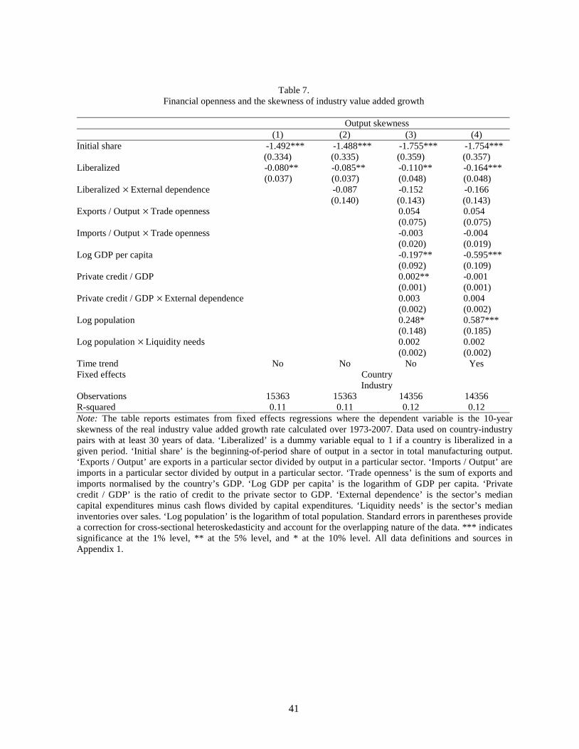
41

Table 7. Financial openness and the skewness of industry value added growth

Output skewness (1) (2) (3) (4)

Initial share -1.492*** -1.488*** -1.755*** -1.754*** (0.334) (0.335) (0.359) (0.357) Liberalized -0.080** -0.085** -0.110** -0.164*** (0.037) (0.037) (0.048) (0.048) Liberalized ×External dependence -0.087 -0.152 -0.166 (0.140) (0.143) (0.143) Exports / Output ×Trade openness 0.054 0.054 (0.075) (0.075) Imports / Output ×Trade openness -0.003 -0.004 (0.020) (0.019) Log GDP per capita -0.197** -0.595*** (0.092) (0.109) Private credit / GDP 0.002** -0.001 (0.001) (0.001) Private credit / GDP ×External dependence 0.003 0.004 (0.002) (0.002) Log population 0.248* 0.587*** (0.148) (0.185) Log population ×Liquidity needs 0.002 0.002 (0.002) (0.002) Time trend No No No Yes Fixed effects Country Industry Observations 15363 15363 14356 14356 R-squared 0.11 0.11 0.12 0.12 Note: The table reports estimates from fixed effects regressions where the dependent variable is the 10-year skewness of the real industry value added growth rate calculated over 1973-2007. Data used on country-industry pairs with at least 30 years of data. ‘Liberalized’ is a dummy variable equal to 1 if a country is liberalized in a given period. ‘Initial share’ is the beginning-of-period share of output in a sector in total manufacturing output. ‘Exports / Output’ are exports in a particular sector divided by output in a particular sector. ‘Imports / Output’ are imports in a particular sector divided by output in a particular sector. ‘Trade openness’ is the sum of exports and imports normalised by the country’s GDP. ‘Log GDP per capita’ is the logarithm of GDP per capita. ‘Private credit / GDP’ is the ratio of credit to the private sector to GDP. ‘External dependence’ is the sector’s median capital expenditures minus cash flows divided by capital expenditures. ‘Liquidity needs’ is the sector’s median inventories over sales. ‘Log population’ is the logarithm of total population. Standard errors in parentheses provide a correction for cross-sectional heteroskedasticity and account for the overlapping nature of the data. *** indicates significance at the 1% level, ** at the 5% level, and * at the 10% level. All data definitions and sources in Appendix 1.

42

Table 8. Financial openness and the skewness of industry-level value added growth: Liberalization intensity

Output skewness (1) (2) (3) (4)

Liberalization intensity -0.082* -0.091* -0.110* -0.283*** (0.045) (0.056) (0.063) (0.077) Liberalization intensity ×External dependence -0.252 -0.386** 0.393*** (0.166) (0.181) (0.171) Industry and country co-variates No No Yes Yes Time trend No No No Yes Fixed effects Country Industry Observations 15363 15363 14356 14356 R-squared 0.11 0.11 0.12 0.12 Note: The table reports estimates from fixed effects regressions where the dependent variable is the 10-year skewness of the real industry value added growth rate calculated over 1973-2007. Data used on country-industry pairs with at least 30 years of data. ‘Liberalization intensity’ is the ratio of International Finance Corporation investable to global market capitalisation after the liberalization year. ‘External dependence’ is the sector’s median capital expenditures minus cash flows divided by capital expenditures. All other industry and country variables and interactions from Table 6 are included in the regression (coefficients not reported for brevity). Standard errors in parentheses provide a correction for cross-sectional heteroskedasticity and account for the overlapping nature of the data. *** indicates significance at the 1% level, ** at the 5% level, and * at the 10% level. All data definitions and sources in Appendix 1.

43

Table 9. Financial openness and the skewness of industry value added growth: Propensity score matching

Output skewness (1) (2) (3) (4)

Liberalized -0.135*** -0.184*** -0.135*** -0.141*** (0.029) (0.045) (0.037) (0.039) Liberalized ×External dependence -0.212*** -0.225*** -0.227*** (0.024) (0.013) (0.013) Industry and country co-variates No No Yes Yes Time trend No No No Yes Fixed effects Country Industry Observations 9631 9631 8955 8955 R-squared 0.05 0.08 0.15 0.15 Note: The table reports estimates from fixed effects regressions where the dependent variable is the 10-year skewness of the real industry value added growth rate calculated over 1973-2007. Data used on country-industry pairs with at least 30 years of data. The control group of non-liberalized countries is selected by a propensity score matching procedure. ‘Liberalized’ is a dummy variable equal to 1 if a country is liberalized in a given period. ‘External dependence’ is the sector’s median capital expenditures minus cash flows divided by capital expenditures. All other industry and country variables and interactions from Table 6 are included in the regression (coefficients not reported for brevity). Standard errors in parentheses provide a correction for cross-sectional heteroskedasticity and account for the overlapping nature of the data. *** indicates significance at the 1% level, ** at the 5% level, and * at the 10% level. All data definitions and sources in Appendix 1.

44

Table 10. Financial openness and the skewness of industry value added growth: Data issues

Output skewness (1) (2) (3)

Liberalized -0.080** -0.102*** (0.040) (0.024) Liberalized ×External dependence -0.173 -0.187*** (0.111) (0.019)

Liberalization intensity -0.231*** (0.073) Liberalization intensity ×External dependence -0.381*** (0.145) Industry and country co-variates Yes Yes Yes Time trend Yes Yes Yes Fixed effects Country Industry Observations 20711 20711 20711 R-squared 0.11 0.11 0.11 Note: The table reports estimates from fixed effects regressions where the dependent variable is the 10-year skewness of the real industry value added growth rate calculated over 1973-2007. Data used on country-industry pairs with at least 20 years of data. The control group of non-liberalized countries is either all non-liberalized countries (columns (1) and (2)), or a sub-set of non-liberalized countries selected by a propensity score matching procedure (column (3)). ‘Liberalized’ is a dummy variable equal to 1 if a country is liberalized in a given period. ‘Liberalization intensity’ is the ratio of International Finance Corporation investable to global market capitalization after the liberalization year. ‘External dependence’ is the sector’s median capital expenditures minus cash flows divided by capital expenditures. All other industry and country variables and interactions from Table 6 are included in the regression (coefficients not reported for brevity). Standard errors in parentheses provide a correction for cross-sectional heteroskedasticity and account for the overlapping nature of the data. *** indicates significance at the 1% level, ** at the 5% level, and * at the 10% level. All data definitions and sources in Appendix 1.

45

Table 11. Financial openness and the skewness of industry capital, TFP, establishments, and employment growth

Capital TFP Establishments Employment (1) (2) (3) (4)

Liberalized -0.077* -0.101* 0.055 -0.161*** (0.047) (0.061) (0.074) (0.061) Liberalized ×External dependence -0.056 -0.052 -0.049 -0.352** (0.144) (0.160) (0.220) (0.147) Industry and country co-variates No No Yes Yes Time trend No No No Yes Fixed effects Country Industry Observations 11444 11141 8504 13338 R-squared 0.10 0.10 0.10 0.12 Note: The table reports estimates from fixed effects regressions where the dependent variable is the 10-year skewness of the real growth rate of industry capital (column (1)), TFP (column (2)), establishments (column (3)) and employment (column (4)), calculated over 1973-2007. ‘Liberalized’ is a dummy variable equal to 1 if a country is liberalized in a given period. ‘External dependence’ is the sector’s median capital expenditures minus cash flows divided by capital expenditures. All other industry and country variables and interactions from Table 6 are included in the regression (coefficients not reported for brevity). Standard errors in parentheses provide a correction for cross-sectional heteroskedasticity and account for the overlapping nature of the data. *** indicates significance at the 1% level, ** at the 5% level, and * at the 10% level. All data definitions and sources in Appendix 1.

46

Appendix 1. Variables and sources

GDP per capita Average of total GDP divided by the population. Source: Penn World Tables. Industry output Total output in a particular industry in a particular country in a particular year, in

constant US dollars. Source: Penn Tables and INDSTAT 2010 Rev. 3. Liberalized Dummy variable equal to 1 following the year in which the country liberalizes its stock

market. Source: Bekaert et al. (2005). Liberalization intensity The ratio of International Finance Corporation investable to global market

capitalization after the liberalization year. Source: Bekaert et al. (2005). Initial share The industry’s share of output out of total manufacturing output in this country for a

particular year. Source: INDSTAT 2010 Rev. 3. Population Total population in the respective country. Source: Penn World Tables. Trade openness Exports and imports divided by GDP. Source: Penn World Tables. Constraints on executive Average index of executive checks and balances on the executive branch of

government. Source: Polity IV. Private credit/GDP Average value of total credits by financial intermediaries to the private sector in each

country, excluding credit by central banks. Source: Beck et al. (2010). Government spending/ Average government spending as a share of total GDP. Source: Penn World Tables. GDP Years of schooling Average years of schooling for the population. Source: Barro-Lee Dataset. External dependence The sector’s median value of capital expenditures minus cash flows divided by capital

expenditures, for mature Compustat firms. Adapted for ISIC Rev. 3 from Cetorelli and Strahan (2006).

Liquidity needs The sector’s median value of total inventories divided by total sales, for mature

Compustat firms. Adapted for ISIC Rev. 3 from Raddatz (2006). Exports/Output Average exports in a particular sector divided by output in a particular sector. Adapted

for ISIC Rev. 3 from Di Giovanni and Levchenko (2007). Imports/Output Average imports in a particular sector divided by output in a particular sector. Adapted

for ISIC Rev. 3 from Di Giovanni and Levchenko (2007).