sizing design sensitivity analysis of dynamic frequency...

Choi, K.K. and Lee, J.H., "Sizing Design Sensitivity Analysis of Dynamic Frequency Response of Vibrating Structures," ASME Journal of Mechanical Design, Vol. 114, No. 1, 1992, pp. 166-173; also presented at the 15th ASME Design Automation Conference, September 1989.

Sizing Design Sensitivity Analysis

of Dynamic Frequency Response of Vibrating Structures

by

Kyung K. Choi and Jae Hwan Lee

Department of Mechanical Engineering and

Center for Computer Aided Design College of Engineering The University of Iowa

Iowa City, Iowa

ABSTRACT

A continuum design sensitivity analysis method of dynamic frequency response of structural systems is developed using the adjoint variable and direct differentiation methods. A variational approach with a non-selfadjoint operator for complex variable is used to retain the continuum elasticity formulation throughout derivation of design sensitivity results. Sizing design variables such as thickness and cross-sectional area of structural components are considered for the design sensitivity analysis. A numerical implementation method of continuum design sensitivity analysis results is developed using postprocessing analysis data of COSMIC/NASTRAN finite element code to get the design sensitivity information of displacement and stress performance measures of the structures. The numerical method is tested using basic structural component such as a plate supported by shock absorbers and a vehicle chassis frame structure for sizing design variables. Accurate design sensitivity results are obtained even in the vicinity of resonance. 1. INTRODUCTION

Dynamic frequency response of mechanical and structural systems is

of interest in design problems that are subjected to harmonically varying external loads caused by the reciprocating power train or other rotating machineries such as motors, fans, compressors, and forging hammers [1]. For example, airplane body and wing structures are subjected to a harmonic load transmitted from the propulsion system. Also, ship vibrations resulting from the propeller and engine excitation can cause noise problem, cracks, fatigue failure of tailshaft, and discomfort to crew. When a machine or any structure oscillates in some form of periodic or random motion, the motion generates alternating pressure waves that propagate from the moving surface at the velocity of sound. For instance, the interior sound pressure in an automobile compartment can occur when the input forces transmitted from road and power train excite the vehicle compartment boundary panels. These motions with frequencies between 20 Hz and 20 KHz stimulate the hearing mechanism of human [2].

1


Many of the published work related with dynamic frequency [3-6] concerns about the optimal design of structures without providing considerable information on the design sensitivity analysis even though design sensitivity is the basic ingredient for the formulation of optimality criteria. A broad review of literature for optimal structural design published from 1962 to 1968 is done by Sheu and Prager [3]. Pierson [4] surveyed the published research work on optimal structural design with dynamic constraints up to the beginning of 1970s. Olhoff [5] surveyed the literature of optimal design of one- or two-dimensional elastic structural components with constraints on the fundamental frequency. Haug [6] reviewed a substantial literature in the area of optimization of distributed parameter structures with constraints on static and dynamic responses.

A variational principle is used by Mroz in deriving necessary and sufficient conditions of optimal design [7]. Lekszycki and Olhoff [8] derived a general set of necessary conditions for an optimal design of one-dimensional, viscoelastic structures acted on by harmonic loads. A non-selfadjoint operator is used by means of variational analysis and the concept of complex stiffness modulus is adopted. Yoshimura performed [9] design sensitivity analysis of the frequency response of machine structures and presented a numerical example of design sensitivity using a simplified structural model of a lathe. Lekszycki and Mroz [10] extended their previous work [8] to find necessary conditions for optimal support reactions to minimize stress or displacement amplitudes. A variational approach with non-selfadjoint operator is used to consider a one-dimensional viscoelastic structure subjected to harmonic loads.

The objective of this paper is to create and develop a unified continuum design sensitivity analysis theory of dynamic frequency response that can be easily implemented using the postprocessing data from established finite element codes. For numerical implementation, COSMIC/NASTRAN is used. 2. VARIATIONAL FORMULATION OF DYNAMIC FREQUENCY RESPONSE PROBLEM

The equation of motion for a linear structural dynamics with viscous

damping has the form [11-12],

m(x,u)z t t(x,u, t ) + c(x,u)z t(x,u, t ) + Auz (x,u, t ) = F(x,u, t ), x ∈ Ω, t ≥ 0 (1) where Ω is the domain of the structure, z(x,u,t) is the displacement, u is the sizing design variable, Au is a linear partial differential operator, m(x,u) and c(x,u) are the mass and viscous damping effects in the structure, respectively, and F(x,u,t) is the applied harmonic load. For harmonic excitation, the forced motion is referred to as the steady-state response and the displacement and phase angle of the steady-state response are called the dynamic frequency response of the system.

To change Eq. 1 into the spatial state equation of dynamic frequency response, define the displacement z(x,u,t) and harmonic loading F(x,u,t) using complex response method [8, 12] as

z(x,u, t ) = z(x,u) e−iα(x ,u) eiωt= [ z1(x,u) − i z2(x,u) ] eiωt = z (2)

(x,u)eiωt

2


and

(3) F(x,u, t ) = f (x,u)eiωt

where z(x,u), z(x,u), f(x,u), ω, and α(x,u) are dynamic frequency response displacement magnitude, complex displacement, harmonic load magnitude, load frequency, and phase angle, respectively. It is assumed that the load frequency ω is constant.

Time-dependency can be eliminated by substituting Eqs. 2 and 3 into Eq. 1 to get the spatial state operator equation

Duz(x,u) ≡ −ω2m(x,u)z(x,u) + i ωc(x,u)z(x,u) + Auz(x,u)

= f (x,u), x ∈ Ω (4) with the appropriate boundary conditions. The corresponding variational equation with viscous damping can be derived as

(5)

bu(z, z) ≡ (Duz, z) = ∫ ∫Ω[ −ω2m(x,u)z + i ωc(x,u)z ] z

_ dΩ + au(z, z)

= ∫ ∫Ωf z_(x,u) dΩ = ” u(z), for al l z ∈ Z

where z_

is the complex conjugate of the kinematically admissible virtual displacement , Z is the space of kinematically admissible virtual displacements, and b and are the energy bilinear and load linear forms, respectively. The scalar product of two complex functions is defined as [13],

z

u(z, z) ” u(z)

(6) ( f (z) , g(z) ) = ∫ ∫Ω

f (z)g(z) dΩ

Structural damping is an example of the viscouse damping that is due

to internal friction within the material or at connections between the structural components. When the damping coefficient is small, as in the case for structures, damping is primarily effective at frequencies in the vicinity of resonance [12]. The variational equation with structural damping effect is

(7)

bu(z, z) ≡ ∫ ∫Ω[ −ω2m(x,u)z ]z

_ dΩ + (1 +i ϕ)au(z, z)

= ∫ ∫Ωf z_(x,u) dΩ = ” u(z), for al l z ∈ Z

where ϕ is the structural damping coefficient.

3


3. SIZING DESIGN SENSITIVITY ANALYSIS

In order to find the relationships between a variation of structural dynamic frequency response and a variation of sizing design variables, the design derivative of the variational governing equation is taken. Explicit design sensitivity formulas of dynamic frequency response performance measures are then obtained using the adjoint variable and direct differentiation methods. 3.1 Design Derivative of the Variational Equation

Consider a damped structural system with the variational equilibrium Eq. 5 corresponding to a given design u. The first design variation of Eq. 5 yields

(8) bu(z′, z) = ” ′δu(z) − b′δu(z, z), for al l z ∈ Zwhere

(9) b′δu(z, z) = ∫ ∫Ω

[ −ω2muz + i ωcuz ]z_

δu dΩ + a′δu(z, z)

and

” ′δu(z) = ∫ ∫Ω

f uz_

δu dΩ

(10)

In Eqs. 9 and 10, fu, mu, and cu denote the derivatives of f, m, and c with respect to the design u, respectively. 3.2 Sizing Design Sensitivity Analysis of Dynamic Performance Measure

A general performance measure representing a wide variety of structural responses can be defined as [11]

Ψ = ∫ ∫Ω

g( z, ∇z, u ) dΩ

(11)

where the function g is continuously differentiable with respect to its

arguments and ∇ . Displacement or slope at a point in a structural component can be written using the Dirac delta measure times the displacement or slope function in the integrand of Eq. 11. The variation of the performance measure with respect to the design variable becomes

z = [ z,1, z,2, z,3 ]T

(12) Ψ′ = ∫ ∫Ω

( gzz′ + g∇z∇z′ + guδu ) dΩ

The design sensitivities of the displacement magnitude and phase angle can also be obtained using the design sensitivity of the complex displacement z. For instance, using the relationship,

4


z = (z1)2+ (z2)2

⎬⎪⎪⎪

⎪⎪⎪⎭

⎫

α = tan-1 ⎝

⎛⎜⎜ z2

z1 ⎠

⎞⎟⎟

(13)

the first variations of z(x,u) and α(x,u) become

z ′ = z1(z1)′ + z2(z2)′z

⎬⎪⎪⎪

⎪⎪⎪⎭

⎫

α′ = z1(z2)′− z2(z1)′

z2

(14)

3.3 Adjoint Variable Method

To obtain an explicit expression for Ψ′ in terms of δu, it is necessary to rewrite the first two terms of Eq. 12 explicitly in terms of δu. Let Da

u be the non-selfadjoint operator corresponding to the operator Du of Eq. 4 such that

(Duz,λ) = (z,Dauλ), for al l z, λ ∈ Z (15)

Then by the definition of bu(•,•) in Eq. 5,

(16)

( z′,Da

uλ ) = bu(z′, λ) = ∫ ∫Ω [−ω2m(x,u)z′ + i ωc(x,u)z′ ]λdΩ + au(z′,λ)

An adjoint equation can be defined as

, bu(λ,λ) = ∫ ∫Ω

( gzλ + g∇z∇λ ) dΩ ≡ ” au( λ ) f or al l λ ∈ Z

(17)

where right side is an adjoint load linear form and a unique solution λ is desired. To take advantage of the adjoint equation, we may evaluate Eq. 17 at λ = z ′, since z Z, to obtain ¯ ′ ∈

bu(z′,λ) = ∫ ∫Ω

( gzz′ + g∇z∇z′ ) dΩ

(18)

which is just the first two terms on the right side of Eq. 12. Similarly, evaluating Eq. 8 at z = λ yields ¯

bu(z′,λ) = ” ′δu(λ) − b′δu(z,λ) (19)

5


Since the left sides of Eqs. 18 and 19 are equal, the desired explicit design sensitivity expression can be obtained as

(20)

Ψ ′ = ” ′δu(λ) − b′δu(z,λ) + ∫ ∫Ω

guδu dΩ

3.4 Direct Differentiation Method

Presuming that the displacement z is known as the solution of Eq. 5, Eq. 8 is a variational equation for the first variation z ′. It can be noted that stiffness matrices of Eqs. 5 and 8 are same and the right side of Eq. 8 can be considered as a pseudo load term. If one perturbs a design parameter to define δu and evaluate the right side of Eq. 8 with the solution z of Eq. 5, then Eq. 8 can be solved numerically to obtain z ′ using the finite element method. The design sensitivity Ψ′ in Eq. 12 can then be evaluated using z ′. The numerical efficiency of the adjoint variable and direct differentiation methods is discussed in Ref. 11. 4. DESIGN COMPONENT

In order to demonstrate the basic idea of implementing design sensitivity analysis results, the energy bilinear and load linear forms of the truss/beam and plane elastic solid/plate design components are derived. The design sensitivity expressions for the dynamic frequency responses such as displacement and stress are obtained using the adjoint variable and direct differentiation methods. 4.1. Truss/Beam Design Component

The energy bilinear form of the truss/beam structural component shown in Fig. 1 with structural damping is

bu(z, z) = ∫L

0−ω2

⎝⎛mzz˜

_ + mJ

hz4z˜

_

4 ⎠⎞dx1 + (1 +i ϕ)∫

L

0(Ehz1,1z˜

_

1,1

+ EI 3z2,11z˜_

2,11 + EI 2z3,11z˜_

3,11 + GJz4,1z˜_

4,1)dx1 (21) where z1, z2, z3, and z4, are an axial displacement, two orthogonal lateral displacements, and an angle of twist, respectively, and

In Eq. 21, E is Young's modulus, G is shear modulus, u=h(x1), I2, I3, and J are cross-sectional area, two moments of inertia and a torsional moment of inertia, respectively. Note that bending and torsional terms are excluded from the energy bilinear form when only the truss component is considered.

z = [z1, z2, z3, z4]T

Fig. 1 Truss/beam Structural Component

6


The load linear form of the external loads shown in Fig. 1 is

” u(z) = ∫

L

0 ⎝

⎛

⎜⎜⎜∑

3

i=1

f i z˜_

i + T1z˜_

4 + M2z˜_

3,1 + M3z˜_

2,1 ⎠

⎞

⎟⎟⎟dx1

(22)

where f1, f2, and f3 are an axial and two orthogonal lateral harmonic loads, respectively. Also, T1 is a harmonic torque and M2 and M3 are two harmonic moments. If only the truss component is considered, torsional load and bending moment are excluded.

The first variations of the energy bilinear and load linear forms of Eqs. 9 and 10 can be taken as

b'δu(z, z) = ∫

L

0−ω2

⎝⎛mhzz˜

_ + ⎝

⎛ mJh ⎠

⎞

hz4z˜

_

4 ⎠⎞δudx1

+ (1 +i ϕ)∫L

0(Ez1,1z˜

_

1,1 + EI3hz2,11z˜_

2,11

+ EI 2hz3,11z˜_

3,11 + GJhz4,1z˜_

4,1)δhdx1 (23) and

” '

δu(z) = ∫L

0 ⎝

⎛

⎜⎜⎜∑

3

i=1

f ih z_

i + T1hz_

4 + M2hz_

3,1 + M3hz_

2,1 ⎠

⎞

⎟⎟⎟δhdx1

(24)

where the subscript h denotes the derivative of terms with respect to the design variable h.

For the adjoint variable method, the design sensitivity of a complex displacement at a discrete point can be obtained from Eq. 20 using Eqs. 23 and 24 where the adjoint equation is given in Eq. 17. For the direct differentiation method, the design sensitivity z ′ of complex displacement can be obtained by solving Eq. 8. For the displacement at any point in an element, the design sensitivity can be obtained by interpolating z ′ at nodal points using the shape function.

Next consider a complex performance measure representing an averaged axial stress over a small subinterval of the beam as

(25) Ψ1 = ∫

L

0E(z1,1 + αh1/ 2z2,11 + βh1/ 2z3,11) mpdx1

where, αh1/2(x1) and βh1/2(x1) are the half-depths of the beam along x2 and x3 axes, respectively, and mp is a characteristic function that is nonzero only on a small subinterval ∆xp,

7


mp(x1) =

1

∫x p

dx1

, x1 ∈ ∆xp

⎨⎪⎪⎪⎪

⎪⎪⎪⎪

⎩

⎧

0 , x1 ∉ ∆xp

(26)

For pointwise stress performance measure, mp(x1) becomes the Dirac delta measure if the small subinterval ∆xp shrinks to a point.

The first variation of the average stress performance measure Ψ1 is

Ψ′1 = ∫L

0E(z′1,1 + αh1/ 2z′2,11 + βh1/ 2z′3,11) mpdx1

+ ∫L

0 ⎝⎛ 1

2αh−1/ 2z2,11 + 1

2βh−1/ 2z3,11 ⎠

⎞δh mpdx1

(27)

The adjoint equation is, in this case,

(28) bu(λ,λ) = ∫

L

0E(λ1,1 + αh1/ 2λ2,11 + βh1/ 2λ3,11) mpdx1

Using the adjoint variable method, the design sensitivity of the complex stress has the form

Ψ'

1 = ” 'δu(λ) − b'

δu(z,λ) + ∫L

0 ⎝⎛ 1

2αh−1/ 2z2,11 + 1

2βh−1/ 2z3,11 ⎠

⎞δhmpdx1

(29)

The design sensitivity of stress performance measure can also be obtained using the direct differentiation method. Once the solution z ′ of Eq. 8 is obtained, the first and second partial derivatives of z ′ with respect to x1 can be numerically evaluated using the shape function. Then, the integrations in Eq. 27 can be carried out to yield the design sensitivity. 4.2 Plane Elastic Solid/Plate Design Component

Consider a plane elastic solid(membrane)/plate structural component of Fig. 2. The sizing design variable u = h(x1,x2) is the thickness of the structural component. The energy bilinear form for the design component with structural damping is

8


bu(z, z) = ∫ ∫Ω−ω2mzz˜

_ dΩ + (1 +i ϕ)au(z, z)

= ∫ ∫Ω−ω2mzz˜

_ dΩ

+ (1 +i ϕ)∫ ∫Ω ⎣

⎡

⎢⎢⎢h∑

2

i, j =1

σij (v )εij (v˜_) + h

3 ∑2

i, j =1

σij (z3)εij (z˜_

3)

⎦

⎤

⎥⎥⎥dΩ

(30) where v = [z1, z2]T for the plane elastic solid component. Note that the bending terms are excluded from the energy bilinear form when only the plane elastic solid structural component is considered.

Fig. 2 Plane Elastic Solid/Plate Structural Component

The load linear form of the external loads shown in Fig. 2 is

” u(z) = ∫ ∫Ω

∑3

i=1

f i z_

i dΩ + ∫Γ2Tv

_ dΓ

(31)

where f1, f2, and f3 are two-inplane and a lateral harmonic loads, respectively, and T = [T1, T2]T is a harmonic traction load. The lateral load is excluded if only the plane elastic solid structural component is considered.

The first variations of the energy bilinear and load linear forms are

b'δu(z, z) = ∫ ∫Ω

−ω2mhzz˜_ δhdΩ

+ (1 +i ϕ)∫ ∫Ω ⎣

⎡

⎢⎢⎢ ∑

2

i, j =1

σij (v)εij (v˜_) + 1

3 ∑2

i, j =1

σij (z3)εij (z˜_

3)

⎦

⎤

⎥⎥⎥δhdΩ

(32) and

(33)

” ′δu(z) = ∫ ∫Ω

∑3

i=1

f ih z_

i δh dΩ

where the subscript h denotes the derivative of terms with respect to the design variable h.

9


As in the truss/beam structural component, for the adjoint variable method, the design sensitivity of a complex displacement at a discrete point can be obtained from Eq. 20 using Eqs. 32 and 33 where the adjoint equation is given in Eq. 17. For the direct differentiation method, the discussion given for the truss/beam component is applicable here.

Consider, unlike the truss/beam component case, a pointwise stress measure on the structural component as

Ψ2 = ∫ ∫Ω

σ11(z) δ(x−x ) dΩ

(34)

where δ is the Dirac delta measure and ˆ

σ11 = E

1 −ν2(z1,1 + νz2,2) − Eh

2 (1 −ν2) ( z3,11 + νz3,22)

(35)

The first variation of the performance measure of Eq. 34 is

Ψ′2 = ∫ ∫Ω

E

1 − ν2 ⎨⎩⎧(z′1,1 + νz′2,2) − h

2(z′3,11 + νz′3,22)

⎬⎭⎫ δ(x−x ) dΩ

− ∫ ∫Ω

E

2 (1 − ν2) (z3,11 + νz3,22)

⎬⎭⎫ δ(x−x ) δh dΩ

(36)

The adjoint equation can be defined as

bu(λ,λ) = ∫∫Ω

E

1 − ν2 ⎨⎩⎧ (λ1,1 + νλ2,2) − h

2(λ3,11 + νλ3,22)

⎬⎭⎫ δ(x−x ) dΩ

(37)

Using the adjoint variable method, the design sensitivity of the complex stress can be obtained as

Ψ′2 = ” ′δu(λ) − b′δu(z,λ) − ∫∫Ω

E

2 (1 − ν2) (z3,11 + νz3,22) δ(x−x ) δh dΩ

(38)

For the direct differentiation method, the discussion given for the truss/beam component is applicable here. 5. NUMERICAL IMPLEMENTATION WITH ESTABLISHED FINITE ELEMENT ANALYSIS CODE

For design sensitivity analysis by the adjoint variable method, the adjoint load for each performance measure needs to be computed. For the displacement performance measure, a unit harmonic load is applied at the specified node of the adjoint structure in the direction of the displacement of which the design sensitivity information is to be computed. To compute the adjoint load associated with a stress performance measure, the shape functions of the finite element method can be used. The adjoint structural

10


response; i.e., the solutions of Eqs. 17, 28, and 37 can be obtained efficiently by the restart option of the established FEM code. Using the original and adjoint structural responses, the design sensitivity information of Eqs. 20, 29, and 38 can be obtained by carrying out numerical integration. Computational procedure for continuum design sensitivity analysis can be found in Refs. 14 and 15.

When design sensitivity analysis is performed by the direct differentiation method, the pseudo load on the right of Eq. 8 is computed using the shape functions and numerical integration. The difficulties involved in numerical implementation for the two methods are the same. An efficient solution of Eq. 8 can also be obtained using the restart option as in the adjoint variable method. Note that the structural response z ′ itself is the design sensitivity information. For the design sensitivity of the stress performance measure, integrations in Eqs. 12, 27, and 36 can be evaluated numerically using the response z ′ and the shape functions. 6. NUMERICAL TEST FOR SIZING DESIGN SENSITIVITY ANALYSIS

The continuum design sensitivity analysis method developed is implemented and tested using finite element analysis code COSMIC/NASTRAN to demonstrate accuracy and efficiency of the method. 6.1 Plate Supported by Shock Absorbers

Consider a plate with shock absorbers as shown in Fig. 3. The plate is 1.02 m x 1.02 m (40 in. x 40 in.) and is loaded with a concentrated vertical dynamic harmonic load at the center. The first three natural frequencies of a plate are 10.94 Hz, 37.76 Hz, and 47.24 Hz. The load magnitude is 44.5 N (10 lb) and two cyclic frequencies ω = 10.8 and ω= 10.9 Hz are considered. Note these cyclic frequencies are very close to the fundamental frequency ωc = 10.94 Hz. Due to symmetry, only one quarter of the plate is analyzed. Young's modulus, mass density, and Poisson's ratio are E = 206.8 GPa (3.0x107 psi), ρ = 20.3 kg/m3 (7.34x10-4

lb/in3) and ν = 0.3, respectively. The spring and damping coefficients are 656.5 kN/m and 17.5 kN-s/m, respectively. The nominal design has uniform thickness 2.54 mm (0.1 in.) and the structural damping is ϕ = 0.04. The governing equation of the plate with shock absorbers can be expressed as

bu(z, z) =∫ ∫Ω

−ω2mzz˜_ dΩ + (1 +i ϕ)∫ ∫Ω

h3 ∑

2

i, j =1

σij (z3)εij (z˜_

3)dΩ

+ ∑

NS

i=1

δ(x−x s) Ki z3z_

3 + ∑ND

i=1

δ(x−x s) i ωCi z3z_

3

(39)

= ∫ ∫Ω

fz_

3dΩ = ” u(z), for al l z ∈ Z

11


Fig. 3 Plate Supported by Shock Absorbers (Coarse Model)

The finite element model consists of 25 square bending elements of COSMIC/NASTRAN QUAD2 [16], 36 nodal points and 108 degrees of freedom. The bending element QUAD2 uses two sets of overlapping basic triangular elements and stresses in the subtriangle are computed at the point of intersection of the diagonals and averaged [17]. The element has both bending and membrane capabilities. However, only the bending capability is considered here. Explicit shape functions are not used for construction of the element stiffness matrix and computation of the bending stress in NASTRAN [17].

To numerically compute design sensitivity, the original displacements and stress, and the adjoint displacements and strains are required as can be seen in Eq. 38. Since QUAD2 element strain information can not be recovered from Direct Frequency Analysis [18] of NASTRAN, the adjoint stress is used with the stress-strain relation. For numerical integration of design sensitivity expressions, it is desirable to use the same shape functions used in the finite element code to interpolate the nodal displacements and stresses at Gauss points. However, there is no explicit shape functions for QUAD2. Moreover, the element stress is recovered at the element centroid only. To alleviate this difficulty, external shape functions are used. That is, once the degrees of freedom of a finite element in NASTRAN is known, compatible shape functions that have the same degrees of freedom can be selected. By employing the external shape functions cited in Refs. 19 or 20, the original and adjoint displacements and stresses are obtained at Gauss points for numerical integration using single precision data recovery of NASTRAN nodal displacements. It is shown in Ref. 15 that design sensitivity accuracy is excellent even if external shape functions are used.

In order to demonstrate accuracy of design sensitivity results in the vicinity of resonance, the design sensitivity analysis is performed with excitation frequencies of 10.8 Hz and 10.9 Hz. Thus, frequency ratios are r = ω/ωc = 0.987 and r = 0.996, respectively. Nine-point Gauss integration is used for numerical integration of design sensitivity expressions. The design sensitivity results of real, imaginary, and maximum displacements, and phase angle for the selected nodal points are shown in Table 1 where ND and Hz denote the node number and load frequency, respectively. The real displacement z1, imaginary displacement z2, maximum displacement z, and phase angle α are denoted by R, I, D, and P, respectively in the table. In all tables, Ψ(u-δu) and Ψ(u+δu) are the values of the performance measures at the perturbed designs u-δu and u+δu, respectively, where δu is the amount of design perturbation.

The central finite difference is denoted by ∆Ψ = [Ψ(u+δu) − Ψ(u-δu)]/2 and Ψ′ is the design sensitivity prediction. The ratio between Ψ′ and ∆Ψ times 100 is used as a measure of accuracy of the design sensitivity computation. That is, the agreement 100 % means that the predicted change is exactly same as the finite difference. When ∆Ψ is too small, this accuracy measure may fail to give correct information because ∆Ψ may lose significant digits. On the other hand, if ∆Ψ is too large, the finite difference may have nonlinear terms in it. To monitor the magnitude of ∆Ψ, the ratio of |∆Ψ/Ψ|x100 (%) is given in all tables.

12


The results shown in Table 1 indicate that the agreement between the design sensitivity predictions and the finite differences for 1% design perturbation is not good due to the highly nonlinear behavior of finite differences. In order to demonstrate that the central finite difference ∆Ψ converges to the predicted change Ψ′ , 0.1% perturbation of design is taken for computation, as shown in Table 2.

Table 1. Design Sensitivity of Plate Supported by Shock Absorbers (Displacement, in.*, coarse model, 1% perturbation)

Table 2. Design Sensitivity of Plate Supported by Shock Absorbers (Displacement, in.*, coarse model, 0.1% perturbation)

Next consider the design sensitivity computation for the bending stress. Since NASTRAN provides element stress at the centroid, the pointwise stress performance is measured at the element centroid. To evaluate design sensitivity of Eq. 38, the adjoint solution of Eq. 37 is required. To compute adjoint load on the right side of Eq. 37 and the design sensitivity expression of Eq. 38, the displacement shape functions cited in Refs. 19 or 20 is used. Nine-point Gauss integration is used for numerical integration. For the pointwise stress σ11, design sensitivity analysis is carried out with 0.1% design perturbation and the results are listed in Table 3. The real, imaginary, and maximum stresses are denoted as R, I, and S, respectively and EL is the element number in the tables. As shown in Table 3, excellent agreement are obtained with |∆Ψ/Ψ| in the range of 1.0~8.5 %.

Table 3. Design Sensitivity of Plate Supported by Shock Absorbers (Stress, psi*, coarse model, 0.1% perturbation)

It is shown in Ref. 21 that, for the shape design variable, more accurate design sensitivity information can be obtained if accurate finite element analysis results are used to evaluate the continuum design sensitivity analysis results. To see whether this is the case for the sizing design variable, a refined finite element model of the quarter plate consisting of 100 square elements QUAD2, with 121 nodal points, and 363 degrees of freedom shown in Fig. 4 is used for numerical computation.

Fig. 4 Plate Supported by Shock Absorbers (refined model)

13


The design sensitivity analysis is performed with 0.1% design

perturbation for the displacement and stress performance measures and the numerical results are given in Tables 4 and 5, respectively. Note that the selected nodes in Table 4 represent the same physical points of the coarse model given in Table 1. The agreements between design sensitivity predictions and the finite differences for displacement and stress in Tables 4 and 5, are consistently improved compared to the results in Tables 2 and 3. Therefore, it can be confirmed that more accurate design sensitivity information can be obtained if accurate finite element results are used to evaluate the continuum design sensitivity analysis results.

Table 4. Design Sensitivity of Plate Supported by Shock Absorbers (Displacement, in.*, refined model, 0.1% perturbation)

Table 5. Design Sensitivity of Plate Supported by Shock Absorbers (Stress, psi*, refined model, 0.1% perturbation)

6.2 Vehicle Chassis Frame Structure A vehicle chassis frame model [22] and a finite element model used

for design sensitivity analysis are shown in Figs. 5 and 6, respectively. The structure is 7.35 m (289.37 in.) long and 0.8 m (31.5 in.) wide with 2 hollow longitudinal frames and 5 hollow cross members. Figure 5 shows the model with suspension coil springs, shock absorbers, linear springs and dampers representing the vehicle tire stiffness and damping effects, respectively, and lumped masses of suspension sprungs. The engine and body masses are attached to the frame by linear springs [23] since these masses are not connected to chassis by welding. The chassis structure is subjected to harmonic loads Fe1, Fe2, and Fe3 excited by the engine of the vehicle. Also, harmonic loads Fs1 and Fs2 are applied to the frame to simulate a sinusoidally varying road surface. Table 6 lists the design specification of mechanical properties, chassis natural frequencies, and loading conditions.

The finite element model contains 2 longitudinal and 5 transverse design components with 68 hollow rectangular beam elements (bold no. 1~68), 13 spring elements, 8 damping elements, 65 nodal points (nonbold no. 1~65), and 15 scalar points (nonbold no. 66~80) including body and engine mount spring attachments with 397 degrees of freedom, as shown in Fig. 6. The nominal design has uniform thickness t = w = 5.08 mm (0.2 in.), width b = 10.16 cm (4.0 in.), and height h = 15.24 cm (6.0 in.). Young's modulus, Poisson's ratio, mass density, and structural damping coefficient are E = 206.8 GPa (3.0x107 psi), ν = 0.3, ρ = 20.3 kg/m3

(7.34x10-4 lb/in3), and ϕ = 0.04, respectively. To prevent vehicle rigid body motion, x1- and x2- displacements at

nodes 24 and 49 are constrained and the ends of spring and damping elements representing tires are fixed on the ground. COSMIC/NASTRAN

14


Direct Frequency Response Analysis is used for the original and adjoint structural finite element analysis.

Table 6. Design Specification for Vehicle Chassis Frame

Fig. 5 Vehicle Chassis Frame Structure

Fig. 6 Finite Element Model of Vehicle Chassis Frame Structure

The variational governing equation of vehicle chassis frame built-up structure is

bu(z, z) = ∑m

i=1

bui (z, z) + ∑NS

i=1

δ(x−xs) Ki z3z_

3 + ∑ND

i=1

δ(x−xs) i ωCi z3z_

3

− ∑

NM

i=1

δ(x−xs) ω2Miz3z_

3 = ∑m

i=1

” ui (z)

= , (40) ” u(z) f or al l z ∈ Z In Eq. 40, NS, ND, and NM indicate the number of springs, dampers, and lumped masses, respectively, and the total number of the structural components is m. Using the design sensitivity analysis method for built-up structures, design sensitivity computation for the displacement with 1% design perturbations on width, height, and thickness is carried out and the results are given in Table 7 for randomly selected nodal points. The design sensitivity results for the averaged maximum bending stress for each element are given in Table 8 for randomly selected finite elements with 1% design perturbation. As seen in Tables 7 and 8, the design sensitivity results are in excellent agreement with the finite differences.

Table 7. Design Sensitivity of Vehicle Chassis Frame (Displacement, in.*)

Table 8. Design Sensitivity of Vehicle Chassis Frame (Stress, psi*)

15


6.5 Comparison of Computation Time For efficiency test, computation CPU time is checked on VAX 11/780

with VMS operating system and listed in Table 9 for the coarse and refined models of the plate supported by shock absorbers. Averaged CPU time is measured for the original structural analysis, adjoint load computation, the first adjoint structural analysis using NASTRAN restart option, additional adjoint analysis, and design sensitivity computation of a stress performance measure. It can be noted from Table 9 that the first adjoint structural analysis of dynamic frequency is not cheap even though restart option is used. However, it becomes inexpensive when the number of performance measures increases since only the first adjoint analysis is expensive. Note that CPU time spent for an additional adjoint structural analysis is quite small.

Table 9. Comparison of CPU time (seconds)

7. CONCLUSION

The continuum sizing design sensitivity analysis results for dynamic frequency response of damped structural systems are numerically implemented using postprocessing analysis data of finite element analysis code COSMIC/NASTRAN. Accurate design sensitivity results are obtained at any frequency range including neighborhood of resonance for both vibrating structures used for numerical test. As noted in Ref. 15, numerical study of the plate supported by shock absorbers indicates that external shape functions that have the same degrees of freedom can be used to evaluate adjoint loads and design sensitivity expressions. That is, use of external shape function does not affect accuracy of the resulting design sensitivities. This is very important for numerical implementation of the continuum design sensitivity analysis results with established FEM codes that do not provide shape functions.

It is found that the design sensitivity results obtained do not agree with the finite difference results near the fundamental frequency when the perturbation ratio |∆Ψ/Ψ| of the performance measure is large. However, in all tested cases, the design sensitivity results agree with the finite difference if design perturbation is reduced so that |∆Ψ/Ψ| becomes smaller. This confirms the fact that there is an uncertainty in the selection of design perturbation amount for the finite difference method in which design sensitivity information are obtained by finite differences.

In Ref. 21, it is shown that more accurate design sensitivity results can be obtained for the shape design variable if accurate finite element analysis results are used. To see whether this is the case for sizing design variables, the coarse and refined models are tested and the results are compared. As demonstrated in Tables 4 and 5 of the refined model, better design sensitivity information can be obtained if improved finite element analysis results are used to evaluate design sensitivity results.

16


REFERENCES 1. Crede, C., Shock and Vibration Concepts in Engineering Design,

Prentice-Hall, Englewood Cliffs, N.J., 1965. 2. Fahy, F., Sound and Structural Vibration, Radiation, Transmission

and Response, Academic Press, N.Y., 1985 3. Sheu, C. Y. and Prager, W., "Recent Developments in Optimal

Structural Design," Appl. Mech. Reviews, Vol. 21, 1968, pp. 985-992. 4. Pierson, B. L., "A Survey of Optimal Structural Design Under

Dynamic Constraints," International J. for Numerical Methods in Engineering, Vol. 4, 1972, pp. 491-499.

5. Olhoff, N., "A Survey of the Optimal Design of Vibrating Structural Elements," Shock and Vibration Digest, Vol. 8, No. 8, 1976, pp. 3-10.

6. Haug, E. J. and Cea, J. Eds., Optimization of Distributed Parameter Structures, Sijthoff & Noordhoff, Alphen aan den Rijn, The Netherlands, 1980.

7. Mroz, Z., "Optimal Design of Elastic Structures Subjected to Dynamic, Harmonically-varying Loads," Zeitschrift fur Angewande Mathematik und Mechanik, Vol. 50, 1970, pp. 303-309.

8. Lekszycki, T. and Olhoff, N., "Optimal Design of Viscoelastic Structures under Forced Steady-State Vibration," J. of Structural. Mech, Vol. 9, No. 4, 1981, pp. 363-387.

9. Yoshimura, M., "Design Sensitivity Analysis of Frequency Response in Machine Structures," ASME, 83-DET-50.

10. Lekszycki, T. and Mroz, Z., "On Optimal Support Reaction in Viscoelastic Vibrating Structures," J. of Structural Mechanics, Vol. 11, No. 1, 1983, pp. 67-79.

11. Haug, E. J., Choi, K. K., and Komkov, V., Design Sensitivity Analysis of Structural Systems, Academic Press, New York, N.Y., 1986.

12. Craig, R. R. Jr., Structural Dynamics, An Introduction to Computer Methods, John Wiley and Sons, N.Y., 1981.

13. Oden, J. T., Applied Functional Analysis, Prentice-Hall, Inc., Englewood Cliffs, N.J., 1979.

14. Choi, K. K., Santos, J.L.T., and Frederick, M. C., "Implementation of Design Sensitivity Analysis with Existing Finite Element Codes," ASME J. of Mechanisms, Transmissions, and Automation in Design, Vol. 109, No. 3, 1987, pp. 385-391.

15. Dopker, B. and Choi, K. K., "Sizing and Shape Design Sensitivity Analysis Using a Hybrid Finite Element Code," Finite Elements in Analysis and Design Vol. 3, 1987, pp. 315-331.

16. NASTRAN, User's Manual Vols. I and II, Cosmic, Computer Services Annex, Univ. of Georgia, Athens, Georgia, 1987.

17. NASTRAN, The NASTRAN Theoretical Manual, National Aeronautics and Space Administration, Washington, D.C., 1981.

18. NASTRAN, The NASTRAN Programmer's Manual, National Aeronautics and Space Administration, Washington, D.C., 1978.

19. Prezemieniecki, J. S., The Theory of Matrix Structural Analysis, McGraw-Hill Book Co., N.Y., 1968.

20. Zienkiewicz, O. C., The Finite Element Method, McGraw-Hill, (UK) Limited, 1979.

21. Choi, K. K. and Twu, S. L., "On Equivalence of Continuum and Discrete Methods of Shape Design Sensitivity Analysis," AIAA, to appear, 1989.

17


22. Sabana, A. and Wehage, A., "Dynamic Analysis of Large Scale Inertia-Variant Flexible Systems," Technical Report No. 82-7, Center for Computer Aided Design, The Univ. of Iowa, Sep., 1982.

23. Kamal, M. M. and Wolf, J. A. Jr, Modern Automotive Structural Analysis, Van Nostrand Reinhold Company, N.Y., 1982.

18

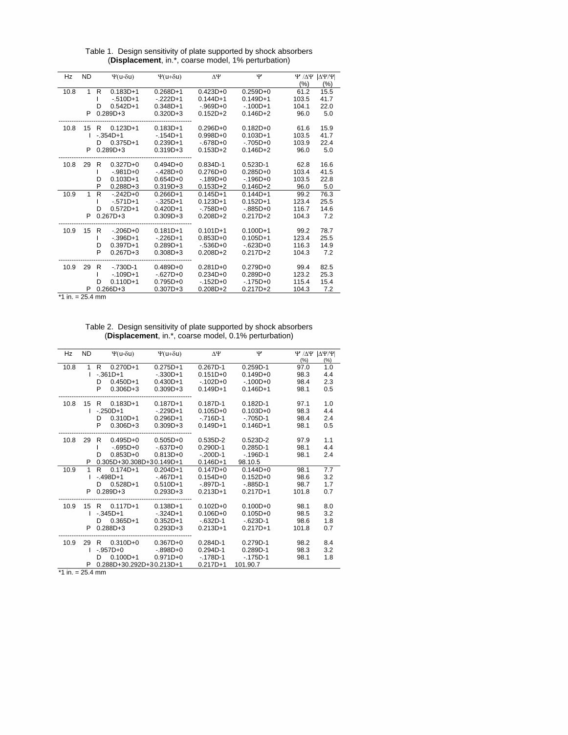
Table 1. Design sensitivity of plate supported by shock absorbers (Displacement, in.*, coarse model, 1% perturbation)

Hz ND Ψ(u-δu) Ψ(u+δu) ∆Ψ Ψ′ Ψ′ /∆Ψ |∆Ψ/Ψ| (%) (%) 10.8 1 R 0.183D+1 0.268D+1 0.423D+0 0.259D+0 61.2 15.5 I -.510D+1 -.222D+1 0.144D+1 0.149D+1 103.5 41.7 D 0.542D+1 0.348D+1 -.969D+0 -.100D+1 104.1 22.0 P 0.289D+3 0.320D+3 0.152D+2 0.146D+2 96.0 5.0 ------------------------------------------------------------- 10.8 15 R 0.123D+1 0.183D+1 0.296D+0 0.182D+0 61.6 15.9 I -.354D+1 -.154D+1 0.998D+0 0.103D+1 103.5 41.7 D 0.375D+1 0.239D+1 -.678D+0 -.705D+0 103.9 22.4 P 0.289D+3 0.319D+3 0.153D+2 0.146D+2 96.0 5.0 ------------------------------------------------------------- 10.8 29 R 0.327D+0 0.494D+0 0.834D-1 0.523D-1 62.8 16.6 I -.981D+0 -.428D+0 0.276D+0 0.285D+0 103.4 41.5 D 0.103D+1 0.654D+0 -.189D+0 -.196D+0 103.5 22.8 P 0.288D+3 0.319D+3 0.153D+2 0.146D+2 96.0 5.0 10.9 1 R -.242D+0 0.266D+1 0.145D+1 0.144D+1 99.2 76.3 I -.571D+1 -.325D+1 0.123D+1 0.152D+1 123.4 25.5 D 0.572D+1 0.420D+1 -.758D+0 -.885D+0 116.7 14.6 P 0.267D+3 0.309D+3 0.208D+2 0.217D+2 104.3 7.2 ------------------------------------------------------------- 10.9 15 R -.206D+0 0.181D+1 0.101D+1 0.100D+1 99.2 78.7 I -.396D+1 -.226D+1 0.853D+0 0.105D+1 123.4 25.5 D 0.397D+1 0.289D+1 -.536D+0 -.623D+0 116.3 14.9 P 0.267D+3 0.308D+3 0.208D+2 0.217D+2 104.3 7.2 ------------------------------------------------------------- 10.9 29 R -.730D-1 0.489D+0 0.281D+0 0.279D+0 99.4 82.5 I -.109D+1 -.627D+0 0.234D+0 0.289D+0 123.2 25.3 D 0.110D+1 0.795D+0 -.152D+0 -.175D+0 115.4 15.4 P 0.266D+3 0.307D+3 0.208D+2 0.217D+2 104.3 7.2 *1 in. = 25.4 mm

Table 2. Design sensitivity of plate supported by shock absorbers

(Displacement, in.*, coarse model, 0.1% perturbation) Hz ND Ψ(u-δu) Ψ(u+δu) ∆Ψ Ψ′ Ψ′ /∆Ψ |∆Ψ/Ψ| (%) (%) 10.8 1 R 0.270D+1 0.275D+1 0.267D-1 0.259D-1 97.0 1.0 I -.361D+1 -.330D+1 0.151D+0 0.149D+0 98.3 4.4 D 0.450D+1 0.430D+1 -.102D+0 -.100D+0 98.4 2.3 P 0.306D+3 0.309D+3 0.149D+1 0.146D+1 98.1 0.5 ------------------------------------------------------------- 10.8 15 R 0.183D+1 0.187D+1 0.187D-1 0.182D-1 97.1 1.0 I -.250D+1 -.229D+1 0.105D+0 0.103D+0 98.3 4.4 D 0.310D+1 0.296D+1 -.716D-1 -.705D-1 98.4 2.4 P 0.306D+3 0.309D+3 0.149D+1 0.146D+1 98.1 0.5 ------------------------------------------------------------- 10.8 29 R 0.495D+0 0.505D+0 0.535D-2 0.523D-2 97.9 1.1 I -.695D+0 -.637D+0 0.290D-1 0.285D-1 98.1 4.4 D 0.853D+0 0.813D+0 -.200D-1 -.196D-1 98.1 2.4 P 0.305D+30.308D+3 0.149D+1 0.146D+1 98.10.5 10.9 1 R 0.174D+1 0.204D+1 0.147D+0 0.144D+0 98.1 7.7 I -.498D+1 -.467D+1 0.154D+0 0.152D+0 98.6 3.2 D 0.528D+1 0.510D+1 -.897D-1 -.885D-1 98.7 1.7 P 0.289D+3 0.293D+3 0.213D+1 0.217D+1 101.8 0.7 ------------------------------------------------------------- 10.9 15 R 0.117D+1 0.138D+1 0.102D+0 0.100D+0 98.1 8.0 I -.345D+1 -.324D+1 0.106D+0 0.105D+0 98.5 3.2 D 0.365D+1 0.352D+1 -.632D-1 -.623D-1 98.6 1.8 P 0.288D+3 0.293D+3 0.213D+1 0.217D+1 101.8 0.7 ------------------------------------------------------------- 10.9 29 R 0.310D+0 0.367D+0 0.284D-1 0.279D-1 98.2 8.4 I -.957D+0 -.898D+0 0.294D-1 0.289D-1 98.3 3.2 D 0.100D+1 0.971D+0 -.178D-1 -.175D-1 98.1 1.8 P 0.288D+30.292D+3 0.213D+1 0.217D+1 101.90.7 *1 in. = 25.4 mm

Table 3. Design sensitivity of plate supported by shock absorbers (Stress, psi*, coarse model, 0.1% perturbation)

Hz EL Ψ(u-δu) Ψ(u+δu) ∆Ψ Ψ′ Ψ′ /∆Ψ |∆Ψ/Ψ| (%) (%) 10.8 1 R 0.327D+5 0.334D+5 0.326D+3 0.316D+3 97.1 1.0 I -.410D+5 -.376D+5 0.168D+4 0.166D+4 98.3 4.3 S 0.525D+5 0.503D+5 -.108D+4 -.106D+4 98.4 2.1 ------------------------------------------------------------- 10.8 13 R 0.177D+5 0.181D+5 0.201D+3 0.195D+3 97.1 1.1 I -.245D+5 -.225D+5 0.101D+4 0.996D+3 98.3 4.3 S 0.303D+5 0.289D+5 -.685D+3 -.674D+3 98.4 2.3 ------------------------------------------------------------- 10.8 25 R 0.386D+4 0.395D+4 0.450D+2 0.446D+2 99.0 1.2 I -.546D+4 -.501D+4 0.225D+3 0.220D+3 97.8 4.3 S 0.669D+4 0.638D+4 -.153D+3 -.149D+3 97.5 2.3 10.9 1 R 0.219D+5 0.253D+5 0.168D+4 0.165D+4 98.1 7.1 I -.566D+5 -.532D+5 0.170D+4 0.168D+4 98.5 3.1 S 0.608D+5 0.589D+5 -.900D+3 -.888D+3 98.7 1.5 ------------------------------------------------------------- 10.9 13 R 0.112D+5 0.132D+5 0.101D+4 0.998D+3 98.1 8.3 I -.339D+5 -.319D+5 0.102D+4 0.100D+4 98.6 3.1 S 0.357D+5 0.345D+5 -.603D+3 -.595D+3 98.7 1.7 ------------------------------------------------------------- 10.9 25 R 0.242D+4 0.287D+4 0.226D+3 0.222D+3 98.3 8.5 I -.754D+4 -.709D+4 0.227D+3 0.222D+3 97.9 3.1 S 0.792D+4 0.765D+4 -.136D+3 -.132D+3 97.4 1.8 *1 psi = 6894.7 Pa

Table 4. Design sensitivity of plate supported by shock absorbers (Displacement, in.*, refined model, 0.1% perturbation)

Hz ND Ψ(u-δu) Ψ(u+δu) ∆Ψ Ψ′ Ψ′ /∆Ψ |∆Ψ/Ψ| (%) (%) 10.8 1 R 0.171D+1 0.201D+1 0.148D+0 0.147D+0 99.3 7.9 I -.497D+1 -.467D+1 0.152D+0 0.151D+0 99.6 3.2 D 0.526D+1 0.508D+1 -.884D-1 -.880D-1 99.6 1.7 P 0.289D+3 0.293D+3 0.214D+1 0.212D+1 99.3 0.7 ------------------------------------------------------------- 10.8 49 R 0.116D+1 0.137D+1 0.104D+0 0.103D+0 99.3 8.2 I -.348D+1 -.327D+1 0.106D+0 0.106D+0 99.6 3.2 D 0.367D+1 0.354D+1 -.630D-1 -.628D-1 99.6 1.7 P 0.288D+3 0.292D+3 0.214D+1 0.212D+1 99.3 0.7 ------------------------------------------------------------- 10.8 97 R 0.322D+0 0.383D+0 0.304D-1 0.302D-1 99.3 8.6 I -.101D+1 -.952D+0 0.308D-1 0.307D-1 99.5 3.1 D 0.106D+1 0.102D+1 -.187D-1 -.186D-1 99.5 1.8 P 0.287D+3 0.291D+3 0.214D+1 0.212D+1 99.3 0.7 10.9 1 R -.310D+0 0.170D+0 0.240D+0 0.239D+099.5 347.4 I -.551D+1 -.549D+1 0.800D-2 0.809D-2101.1 0.1 D 0.552D+1 0.549D+1 -.110D-1 -.111D-1100.5 0.2 P 0.266D+3 0.271D+3 0.249D+1 0.249D+1100.0 0.9 ------------------------------------------------------------- 10.9 49 R -.256D+0 0.807D-1 0.168D+0 0.167D+099.5 193.0 I -.386D+1 -.385D+1 0.538D-2 0.543D-2100.9 0.1 D 0.386D+1 0.385D+1 -.920D-2 -.922D-2100.1 0.2 P 0.266D+3 0.271D+3 0.249D+1 0.249D+1100.0 0.9 ------------------------------------------------------------- 10.9 97 R -.912D-1 0.678D-2 0.490D-1 0.487D-199.5 116.4 I -.112D+1 -.111D+1 0.136D-2 0.135D-299.3 0.1 D 0.112D+1 0.111D+1 -.320D-2 -.318D-299.2 0.3 P 0.265D+3 0.270D+3 0.250D+1 0.250D+1100.1 0.9 *1 in. = 25.4 mm

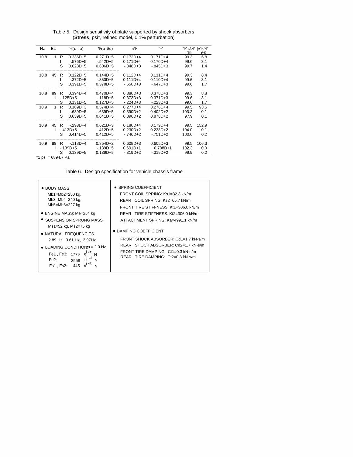
Table 5. Design sensitivity of plate supported by shock absorbers (Stress, psi*, refined model, 0.1% perturbation)

Hz EL Ψ(u-δu) Ψ(u+δu) ∆Ψ Ψ′ Ψ′ /∆Ψ |∆Ψ/Ψ| (%) (%) 10.8 1 R 0.236D+5 0.271D+5 0.172D+4 0.171D+4 99.3 6.8 I -.576D+5 -.542D+5 0.171D+4 0.170D+4 99.6 3.1 S 0.623D+5 0.606D+5 -.848D+3 -.845D+3 99.7 1.4 ------------------------------------------------------------- 10.8 45 R 0.122D+5 0.144D+5 0.112D+4 0.111D+4 99.3 8.4 I -.372D+5 -.350D+5 0.111D+4 0.110D+4 99.6 3.1 S 0.391D+5 0.378D+5 -.650D+3 -.647D+3 99.6 1.7 ------------------------------------------------------------- 10.8 89 R 0.394D+4 0.470D+4 0.380D+3 0.378D+3 99.3 8.8 I -.125D+5 -.118D+5 0.373D+3 0.371D+3 99.6 3.1 S 0.131D+5 0.127D+5 -.224D+3 -.223D+3 99.6 1.7 10.9 1 R 0.189D+3 0.574D+4 0.277D+4 0.276D+4 99.5 93.5 I -.639D+5 -.639D+5 0.390D+2 0.402D+2 103.2 0.1 S 0.639D+5 0.641D+5 0.896D+2 0.878D+2 97.9 0.1 ------------------------------------------------------------- 10.9 45 R -.298D+4 0.621D+3 0.180D+4 0.179D+4 99.5 152.9 I -.413D+5 -.412D+5 0.230D+2 0.238D+2 104.0 0.1 S 0.414D+5 0.412D+5 -.746D+2 -.751D+2 100.6 0.2 ------------------------------------------------------------- 10.9 89 R -.118D+4 0.354D+2 0.608D+3 0.605D+3 99.5 106.3 I -.139D+5 -.139D+5 0.691D+1 0.708D+1 102.3 0.0 S 0.139D+5 0.139D+5 -.319D+2 -.319D+2 99.9 0.2 *1 psi = 6894.7 Pa

Table 6. Design specification for vehicle chassis frame

FRONT SHOCK ABSORBER: Cd1=1.7 kN-s/m REAR SHOCK ABSORBER: Cd2=1.7 kN-s/m

FRONT TIRE STIFFNESS: Kt1=306.0 kN/mREAR TIRE STIFFNESS: Kt2=306.0 kN/m

SPRING COEFFICIENT

DAMPING COEFFICIENT

FRONT COIL SPRING: Ks1=32.3 kN/mREAR COIL SPRING: Ks2=65.7 kN/m

ATTACHMENT SPRING: Ka=4991.1 kN/m

FRONT TIRE DAMPING: Ct1=0.3 kN-s/mREAR TIRE DAMPING: Ct2=0.3 kN-s/m

BODY MASSMb1=Mb2=250 kg, Mb3=Mb4=340 kg,Mb5=Mb6=227 kg

ENGINE MASS: Me=254 kg

SUSPENSION SPRUNG MASSMs1=52 kg, Ms2=75 kg

NATURAL FREQUENCIES

= 2.0 Hz

2.89 Hz, 3.61 Hz, 3.97Hz

LOADING CONDITION:

N

Fs1 , Fs2:

Fe1 , Fe3:

445Fe2: 3558 ei tω

N

ω

1779N

ei tω

ei tω

Table 7. Design sensitivity of vehicle chassis frame (Displacement, in.*) ND Ψ(u-δu) Ψ(u+δu) ∆Ψ Ψ′ Ψ′ /∆Ψ (%) 5 D 0.599D+1 0.609D+1 0.472D-1 0.472D-1 99.8 P 0.310D+3 0.313D+3 -.478D+0 -.478D+0 99.9 10 D 0.410D+1 0.417D+1 0.369D-1 0.368D-1 99.6 P 0.311D+3 0.310D+3 -.467D+0 -.466D+0 99.7 15 D 0.202D+1 0.207D+1 0.228D-1 0.227D-1 99.5 P 0.304D+3 0.303D+3 -.480D+0 -.479D+0 99.7 20 D 0.501D+0 0.510D+0 0.445D-2 0.443D-2 99.6 P 0.193D+3 0.194D+3 0.485D+0 0.487D+0 100.3 25 D 0.288D+1 0.291D+1 0.172D-1 0.170D-1 99.1 P 0.144D+3 0.144D+3 -.273D+0 -.271D+0 99.4 52 D 0.712D+1 0.723D+1 0.519D-1 0.519D-1 100.0 P 0.315D+3 0.314D+3 -.489D+0 -.489D+0 100.0 55 D 0.528D+1 0.537D+1 0.438D-1 0.436D-1 99.7 P 0.313D+3 0.312D+3 -.473D+0 -.472D+0 99.8 58 D 0.289D+1 0.295D+1 0.289D-1 0.288D-1 99.6 P 0.308D+3 0.307D+3 -.471D+0 -.469D+0 99.7 61 D 0.118D+1 0.121D+1 0.167D-1 0.166D-1 99.6 P 0.295D+3 0.295D+3 -.483D+0 -.482D+0 99.7 64 D 0.184D+1 0.186D+1 0.956D-2 0.947D-2 99.0 P 0.149D+3 0.149D+3 -.200D+0 -.198D+0 99.1 *1 in. = 25.4 mm

Table 8. Design sensitivity of vehicle chassis frame (Stress, psi*)

EL Ψ(u-δu) Ψ(u+δu) ∆Ψ Ψ′ Ψ′ /∆Ψ (%) 4 S 0.334D+4 0.318D+4 -.842D+2 -.841D+2 99.9 8 S 0.304D+4 0.286D+4 -.876D+2 -.874D+2 99.7 12 S 0.183D+4 0.172D+4 -.561D+2 -.560D+2 99.8 16 S 0.893D+3 0.843D+3 -.246D+2 -.246D+2 99.7 20 S 0.240D+3 0.243D+3 0.142D+1 0.136D+1 96.2 50 S 0.714D+3 0.677D+3 -.183D+2 -.201D+2 109.5 *1 psi = 6894.7 Pa

Table 9. Comparison of CPU time (seconds)

Original Structural Analysis

Adjoint Load Computation

1st Adjoint Analysis

An Additional Adjoint Analysis

Sensitivity Computation

251 425

0.9 2.1

152 207

9.7 19.2

5.0 20.0

Coarse Model Refined Model

Figure 1

x 2

x3, z3

, z 2

x 1, z 10 L

iωtx13f e( )iωtx11f e( )

iωtx12f e( )

iωtx11T e( )

iωtx1 e( )3M

iωtx1 e( )2Mz4

Figure 2

x 2, z 2

x 3, z 3

2Γ

x1, z 1

Γ

iωtx2x 1 e( , )iωtx2x 13f e( , )

f 2

iωtx2x 1 e( , )f1

iωtx2x 1 e( , )T

Figure 3

x2

x 3

x1ck

17

1319

25

•1

••

•

•8

2229

36

15•

kk

k

k k k

cc

c

c c c

40 in.

40 in.

0

iωtx2x 13f e( , )

Figure 4

k

k c

cx 1

x 3

•

•

•

•

•

•

25

1

49

73

97

1

23

45

67

89

121

x2

20 in.

20 in.

iωt

0

x2x 13f e( , )

Figure 5

t = 0

.2"

h =

6"

b =

4"

w =

0.2

" Cro

ss s

ectio

n of

fram

e

Mb1

Mb2

Mb5

Mb6

Mb3

Mb4

Ms1

Ks1

Cd1

Ct1

Kt1

Cd1

Me

Ms2

Ks2

Cd2

Ct2

Kt2

Ms2

Ks2

Cd2

Fe1

Fe3

Fe2

Fs2

Fs2

Fs1

Fs1

Ka

x 3

x1

x2

Figure 6

5

15

25

52

58

64

30

50

48

1216

501

26

•

•

•

•

•

•

•

•

•

•

•x

x

x

o1

2

3

20

•

•

•

66

67

68

69

•

•

24

49•

•

20

10 •

• 55

61

sizing design sensitivity analysis of dynamic frequency...

Documents