site characteristics associated with conventional and
TRANSCRIPT
Graduate Theses, Dissertations, and Problem Reports
2016
Site Characteristics Associated with Conventional and Site Characteristics Associated with Conventional and
Unconventional Petroleum Development in West Virginia Unconventional Petroleum Development in West Virginia
Frederick Christian Zinkhan Jr.
Follow this and additional works at: https://researchrepository.wvu.edu/etd
Recommended Citation Recommended Citation Zinkhan Jr., Frederick Christian, "Site Characteristics Associated with Conventional and Unconventional Petroleum Development in West Virginia" (2016). Graduate Theses, Dissertations, and Problem Reports. 7056. https://researchrepository.wvu.edu/etd/7056
This Thesis is protected by copyright and/or related rights. It has been brought to you by the The Research Repository @ WVU with permission from the rights-holder(s). You are free to use this Thesis in any way that is permitted by the copyright and related rights legislation that applies to your use. For other uses you must obtain permission from the rights-holder(s) directly, unless additional rights are indicated by a Creative Commons license in the record and/ or on the work itself. This Thesis has been accepted for inclusion in WVU Graduate Theses, Dissertations, and Problem Reports collection by an authorized administrator of The Research Repository @ WVU. For more information, please contact [email protected].
Site Characteristics Associated with Conventional and Unconventional Petroleum Development in West Virginia
Frederick Christian Zinkhan Jr.
Thesis submitted to the Davis College of Agriculture, Natural Resources and Design at West Virginia
University
in partial fulfillment of the requirements for the degree of
Master of Science in Forestry
Shawn Grushecky, Ph.D. Ben Spong, Ph.D.
Michael Strager, Ph.D. Nicolas Zegre, Ph.D.
Division of Forestry and Natural Resources
Morgantown, West Virginia 2016
Keywords: Conventional Unconventional Natural Gas Development
Copyright 2016 Frederick Christian Zinkhan Jr.
ii
Abstract
Site Characteristics Associated with Conventional and Unconventional Petroleum Development in West Virginia
Frederick Christian Zinkhan Jr.
Little research has been done on the characteristics of surface disturbance between conventional
(C) and unconventional (UC) wells in West Virginia. To understand the impacts of petroleum
development in West Virginia, a total of 296 conventional wells and 206 unconventional wells were
digitized for the purposes of this study. Using a combination of spatial and resource-related data, the total
land area impacted, forest fragmentation characteristics, and forest resource impacts were investigated
between conventional and unconventional wells. A metric was developed to understand natural gas
production per land area disturbed for both conventional and unconventional wells. The absolute
magnitude of the footprint associated with the disturbed area of WV forestland in conjunction with four
years (2009 to 2012) of gas-production activity was rather modest. An estimated 2,358 hectares were
disturbed, of which 1,341 hectares were forested. About 73.3% of the estimated forest area removed was
the result of unconventional production and 26.7% was the result of conventional production. The results
indicate that the volume of gas production per unit of area disturbed was much greater for unconventional
wells than conventional wells. The potential for greater production per unconventional well and the
possibility of multiple unconventional wells per pad can be more beneficial to overall surface disturbance,
than the conventional development needed to equal the same amount of unconventional production.
Thus, public policies and regulations limiting the expansion of unconventional wells may have negative
consequences associated with the magnitude of surface disturbance. Interestingly, in contrast to C wells
and studies of UC wells in other regions, the findings for WV suggest that UC wells were most frequently
on already-perforated forests, not on core forests. Thus, the impact on forest fragmentation in WV may
be less than generally anticipated in other regions by some scientists.
iii
Table of Contents Abstract .......................................................................................................................................... ii
Tables: ........................................................................................................................................... iv
Figures: .......................................................................................................................................... v
List of Acronyms: ........................................................................................................................ vii
Introduction: ................................................................................................................................. 1 - Hypotheses ............................................................................................................................... 6
Methodology: ................................................................................................................................. 7 - Spatial methods ....................................................................................................................... 7 - Land Cover .............................................................................................................................. 9 - ELUs ....................................................................................................................................... 10 - Forest Cover .......................................................................................................................... 11 - Forest Fragmentation ........................................................................................................... 12 - Natural Gas Production ....................................................................................................... 13 - Analyses ................................................................................................................................. 14
Results: ......................................................................................................................................... 15 - Relative Impacts on Surface Conditions ............................................................................. 21 - Relative Gas Production per Unit of Area Disturbed ........................................................ 32
Discussion: ................................................................................................................................... 34
Bibliography: ............................................................................................................................... 39
iv
Tables:
Table 1 - Area (ha) for various disturbances for both conventional and unconventional wells in WV, between 2009 and 2012. .............................................................................................................................23 Table 2 - Production and calculated metrics for conventional and unconventional gas wells, from 2009-2012 in WV. .......................................................................................................................................32 Table 3 - Number of sampled drilling sites in WV with multiple wells on a single well pad, 2009-2012..............................................................................................................................................................33
v
Figures:
Figure 1 – Extent and depth to the Marcellus Shale in WV and Pennsylvania (MCOR, 2016). ..........2 Figure 2 - An example of pre- natural gas development of a well site used in this study in WV. The black line denotes the post- development extent of the well site. The orange line denotes the 15-ha buffer zone. ...................................................................................................................................................9 Figure 3 – An example of post- natural gas development of a well site used in this study in WV. The black line denotes the extent of the well site. The orange line denotes the 15-ha buffer zone. ............9 Figure 4 - Total number of unconventional wells spudded from 2009-2012 in WV. ...........................15 Figure 5 - Total number of conventional wells spudded from 2009-2012 in WV. ...............................16 Figure 6 - Mean horizontal well bore length for unconventional gas wells spudded from 2009-2012 in WV (WVGES, 2014). .............................................................................................................................17 Figure 7 - Mean total well bore length conventional gas wells spudded from 2009-2012 in WV (WVGES, 2014). .........................................................................................................................................17 Figure 8 - Mean natural gas production in thousand cubic feet per day (MCF/day) for unconventional gas wells spudded from 2009-2012 in WV. ...................................................................18 Figure 9 - Mean natural gas production in thousand cubic feet per day (MCF/day), per conventional and unconventional gas well spudded from 2009-2012 in WV. ......................................18 Figure 10 - Mean oil production in BOPD for unconventional gas wells spudded from 2009-2012 in WV. ..............................................................................................................................................................19 Figure 11 - Total number of gas wells digitized and included in the analysis of conventional and unconventional well surface impacts in WV. ..........................................................................................19 Figure 12 - Sample of conventional gas wells used in this study, from 2009-2012 in WV. .................20 Figure 13 - Sample of unconventional gas wells used in this study, from 2009-2012 in WV. .............21 Figure 14 - Overview of disturbed areas for conventional gas wells, from 2009-2012 in WV. ...........22 Figure 15 - Overview of disturbed areas for unconventional gas wells, from 2009-2012 in WV. ......22 Figure 16 - Compositions of the ecological land unit percentages found for conventional and unconventional gas wells, from 2009-2012 in WV. .................................................................................25 Figure 17 - Percent forest fragmentation class of conventional and unconventional wells from 2009-2012 in WV. ................................................................................................................................................26 Figure 18 - Total CM disturbed per well type (conventional and unconventional), from 2009-2012 in WV. ..............................................................................................................................................................27 Figure 19 - Total CM disturbed per county for conventional and unconventional gas wells, from 2009-2012 in WV. .......................................................................................................................................27 Figure 20 - Total BM (short tons) disturbed per county for conventional and unconventional gas wells, from 2009-2012 in WV. ...................................................................................................................28 Figure 21 - Total BM (short tons) disturbed per well type (conventional and unconventional), from 2009-2012 in WV. .......................................................................................................................................28 Figure 22 - Monetary value (USD) of the disturbed timber per county for conventional and unconventional gas wells, from 2009-2012 in WV. .................................................................................30 Figure 23 - Monetary value (USD) of the disturbed timber per species for conventional and unconventional gas wells, from 2009-2012 in WV. .................................................................................30

vi
Figure 24 – Total monetary value (USD) of the disturbed timber for conventional and unconventional gas wells, from 2009-2012 in WV. .................................................................................31 Figure 25 - Percent of combined total production (MCF)/overall disturbed (ha) for conventional and unconventional gas wells, from 2009-2012 in WV. ..........................................................................33
vii
List of Acronyms:
AHC Appalachian Hardwood Center
API American Petroleum Institute
BCG Boston Consulting Group
BF Board Feet
BM Biomass
C Conventional
CM Cubic Meter
ELUs Ecological Land Units
FIA Forest Inventory and Analysis
FIDO Forest Inventory Data Online
ha Hectare
HBS Harvard Business School
MBF Thousand Board Feet
MCF Thousand Cubic Feet
MCOR Marcellus Center for Outreach & Research
MMCF Million Cubic Feet
SAMB Statewide Addressing and Mapping Board
UC Unconventional
US United States
USD United States Dollar
USDA-NAIP
United States Department of Agriculture-National Agriculture Imagery Program
USEIA United States Energy Information Administration
WV West Virginia
WVDEP West Virginia Department of Environmental Protection
WVGES West Virginia Geological and Economic Survey
WVGISTCD West Virginia Geographic Information System Technical Center Database
WVSORO West Virginia Surface Owners’ Rights Organization
1
Introduction:
Natural gas represents an important component of national energy supply. In 2015, natural gas
accounted for about 32.7% of primary energy consumed in the US (USEIA, 2016a). Its increase in
relative importance is attributable to the expansion of shale-gas production. Withdraws of natural gas
from shale reserves in the US increased by 6.9 times from 2007 to 2014 (1,990,145 MMCF to 13,754,150
MMCF) (USEIA, 2016b). Over the same period, the proportion of gross natural gas withdraws sourced
from shale-gas wells jumped from 8.1% to 34.9% (USEIA, 2014a).
Conventional (C) wells only use a vertical drilling method to extract resources, whereas
unconventional (UC) wells use a combination of vertical and horizontal drilling methods to extract
resources. According to West Virginia Department of Environmental Protection (WVDEP) well reports,
there are have been a total, both C and UC, of 115,301 wells drilled in WV since 1935. In contrast,
Pennsylvania has had a total of 266,903 wells drilled since at least 1800 (Pennsylvania DEP, 2016).
Much of West Virginia (WV) is included in the Marcellus Shale Formation (Messer, 2008). The
Marcellus Shale is the most expansive shale opportunity being explored in the US (Kargbo et al., 2010).
WV also sits upon the Utica shale formation and upper Devonian resources, which will be explored in the
very near future (Downing, 2014). The Marcellus Shale Formation is considered one of the principal
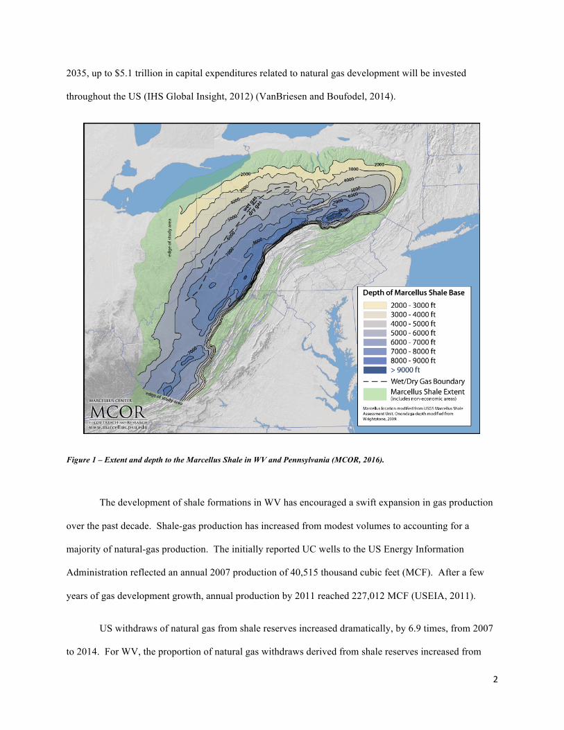
plays in the United States. As shown in Figure 1, the Marcellus Shale Formation natural gas deposit
covers a region ranging from WV on the southern end to upstate New York on the northern end (Soeder
and Kappel, 2009). Its economic potential for the region could be significant (Higginbotham et al., 2010).
For WV alone, Considine et al. (2010) estimated that the value added, or contribution to state domestic
product, will range from $1 billion to $3 billion by 2020, with $1.8 billion representing a medium-
development scenario. With respect to employment impact, the latter study indicated that the range in
jobs created by 2020 would be approximately 15,000 to 44,000, with 26,000 reflecting the medium-
development scenario. In Pennsylvania between 2007 and 2012, the Commonwealth gained over 15,000
jobs in the oil and gas business (Cruz et al., 2014). More recent research estimates that between 2012 and
2
2035, up to $5.1 trillion in capital expenditures related to natural gas development will be invested
throughout the US (IHS Global Insight, 2012) (VanBriesen and Boufodel, 2014).
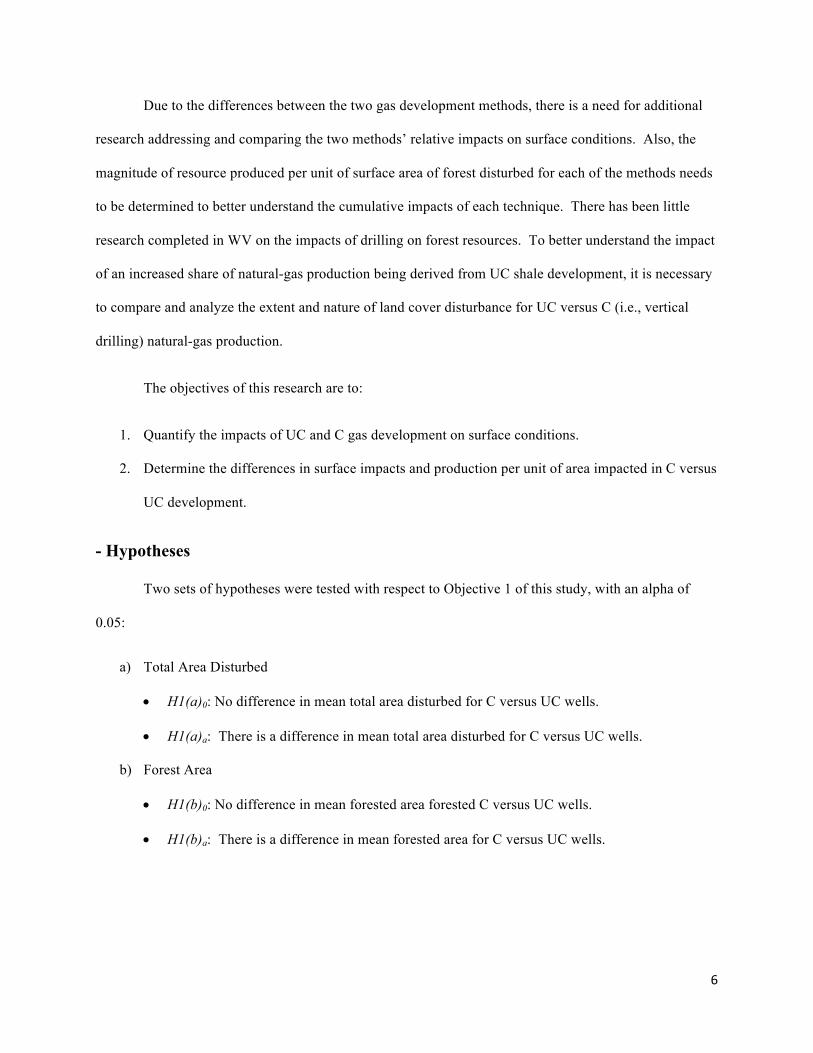
Figure 1 – Extent and depth to the Marcellus Shale in WV and Pennsylvania (MCOR, 2016).
The development of shale formations in WV has encouraged a swift expansion in gas production
over the past decade. Shale-gas production has increased from modest volumes to accounting for a
majority of natural-gas production. The initially reported UC wells to the US Energy Information
Administration reflected an annual 2007 production of 40,515 thousand cubic feet (MCF). After a few
years of gas development growth, annual production by 2011 reached 227,012 MCF (USEIA, 2011).
US withdraws of natural gas from shale reserves increased dramatically, by 6.9 times, from 2007
to 2014. For WV, the proportion of natural gas withdraws derived from shale reserves increased from
3
17.5% to 76.6% during the same time period. With its faster pace of growth, WV’s share of national
shale-gas production increased from 2% in 2007 to 5.8% in 2014 (USEIA, 2014a).
Utilization of shale reserves through directional drilling and hydraulic fracturing has contributed
to the substitution of natural gas for coal in the generation of electricity in the US. The proportion of
national electricity generation fueled by coal decreased from about half in 2005 to just more than a third
by 2013 (McElroy and Lu, 2013). Since coal produces about twice as much carbon dioxide (CO2) as
natural gas per unit of electricity generated (Kargbo et al., 2010), this change in relative consumption
contributed to lower-than-otherwise CO2 emissions (USEIA, 2014b).
Other emission benefits relative to burning coal include lower levels of sulfur dioxide (SO2),
nitrogen oxide (NOx), carbon monoxide (CO), and mercury (Hg) (Kargbo et al., 2010). However, other
concerns regarding the potential negative environmental impacts associated with hydraulic fracturing are
well documented (Zoback et al., 2010; Mckay et al., 2011) such as methane contamination of drinking
water (Osborn et al. 2011; Rahm and Riha, 2012; Hatzenbuhler et al., 2012), seismic risks (Zobac et al.,
2010), unintended release of methane into the atmosphere (Lavelle, 2012; McElroy and Lu, 2013),
intensive consumption of water (Kargbo et al., 2010; Rozell and Reaven, 2012), and hazards associated
with both formation chemicals and introduced chemicals (Kargbo et al., 2010; Hatzenbuhler et al., 2012).
There has been some research indicating that fracking is safe and can be good for the environment. A
recent collaborative report, between the Harvard Business School (HBS) and the Boston Consulting
Group (BCG) (Porter et al., 2015; HBS and BCG 2015), states that natural gas development is the only
viable chance the US has to reduce its greenhouse gas emissions by 2030, while still allowing some
renewable energy sources to penetrate into the industry.
The unintended release of methane into the atmosphere due to leaking pipelines or wells creates
an issue with respect to gas development. Methane typically comprises 95% of natural gas (Union Gas,
2016). During the lifetime of a shale gas well, through venting and leaks, anywhere between 3.6% and
4
7.9% of the methane produced can escape into the atmosphere (Howarth et al., 2011). Methane gas is a
greenhouse gas, and lasts for up to 9.6 years (residence time) in the atmosphere (USEPA and ERG, 2010).
The residence time would be longer if there was a large release of methane into the atmosphere.
Increased natural gas exploration and production also has the potential to impact land cover and
forest resources. These effects are mainly due to the development of pads, roads, and pipelines. In their
analysis of shale-gas development in Pennsylvania, Drohan et al. (2012a) estimated that permits as of
mid-2011 would result in conversion of up to 1,072 hectares of agricultural land and up to 894 hectares of
forestland. Given the differential in forest cover between WV (79%) and Pennsylvania (58.6%) (US
Forest Service, 2012), it is likely that a given gas-production project would impact more forestland in WV
versus those reported by Drohan et al. (2012a) in Pennsylvania.
In a preliminary research project in WV, Grushecky and Wang (2013) found more surface
disturbance per pad (3.0 hectares) than the maximum presumed by Drohan et al. (2012a) (2.0 hectares per
pad) in Pennsylvania. Of the impacted area in WV, almost 63% had been in forest cover. Given the
greater proportion of forested area in WV, Grushecky and Wang’s results also suggested a higher
likelihood of pads in forested area than estimated by Drohan et al. (2012a) in Pennsylvania. While the
Grushecky and Wang (2013) research documented surface impacts, it reported results from only 35 sites
in four counties in WV.
Research has documented that development has affected the level of forest fragmentation in the
Eastern US (Riitters et al., 2012). Caused principally by land-use changes, such fragmentation can yield
lower biodiversity values (Abrahams et al., 2015). Fragmentation potentially impacts ecological and
hydrological processes and thus affects such outcomes as pollution, wildlife movement, and distribution
of invasive species (Riitters et al., 2002). Natural gas development has the potential to disrupt natural
contiguous areas with various land breaks, so it is important to determine where and to what extent forest
fragmentation is occurring (Klaiber et al., 2016). UC shale-gas development has been shown as a
5
process that can impact forest fragmentation (Abrahams et al., 2015). In a simulation study in Quebec,
Racicot et al. (2014) found that shale-gas exploitation would not materially contribute to the loss of forest
cover (i.e., less than 1% loss of forest cover in that case). However, they did find that this development
activity would impact the nature of core forests, increasing the number of forest patches by 13 – 21%.
They found that the pipeline network associated with the projects impacted land cover more than
incremental access roads. Their study area, however, was highly fragmented by roads even prior to the
shale-gas development.
Understanding that some of the areas disturbed by gas development were once forestland, it is
important to determine the value and quantity of what was removed. As noted earlier, forests account for
almost 80% of the land cover in WV (Widmann, 2013). The forests are dominated by hardwood species,
such as yellow-popular, chestnut oak, red maple, white oak, northern red oak, sugar maple, black oak,
American beech, black cherry, and pignut hickory. This is important, because most forests in WV are
made up of older trees and not just smaller stems such as saplings. Most of the forestland in the state is
privately owned. Private ownership accounts for 87% of the forestland area, with public ownership
representing just 13% of the area (Widmann, 2013).
Conventional petroleum development in WV has been around since the early 19th century
(Thoenen, 1964). Some of the first petroleum producing wells were bored near Burning Springs, WV.
The petroleum was a byproduct related to salt production (WVGES, 2004). In 1815, natural gas was first
extracted from a salt well located in Charleston, WV (Callahan, 1923). The first well to be drilled solely
for petroleum was permitted in 1859 (WVGES, 2004). UC wells typically use larger development
equipment and impact more area than C wells. According to WVDEP permit data, UC petroleum
development consisting of horizontal boreholes initiated in WV in the late 1990s to early 2000s. This
drilling technology expanded greatly after 2007 in WV and now has become the dominant form of
drilling in the state.
6
Due to the differences between the two gas development methods, there is a need for additional
research addressing and comparing the two methods’ relative impacts on surface conditions. Also, the
magnitude of resource produced per unit of surface area of forest disturbed for each of the methods needs
to be determined to better understand the cumulative impacts of each technique. There has been little
research completed in WV on the impacts of drilling on forest resources. To better understand the impact
of an increased share of natural-gas production being derived from UC shale development, it is necessary
to compare and analyze the extent and nature of land cover disturbance for UC versus C (i.e., vertical
drilling) natural-gas production.
The objectives of this research are to:
1. Quantify the impacts of UC and C gas development on surface conditions.
2. Determine the differences in surface impacts and production per unit of area impacted in C versus
UC development.
- Hypotheses
Two sets of hypotheses were tested with respect to Objective 1 of this study, with an alpha of
0.05:
a) Total Area Disturbed
• H1(a)0: No difference in mean total area disturbed for C versus UC wells.
• H1(a)a: There is a difference in mean total area disturbed for C versus UC wells.
b) Forest Area
• H1(b)0: No difference in mean forested area forested C versus UC wells.
• H1(b)a: There is a difference in mean forested area for C versus UC wells.
7
In addition, one hypothesis will be tested with respect to Objective 2 of this study, with an alpha
of 0.05:
• H20: No difference in mean production per ha of total area disturbed for C versus UC wells.
• H2a: There is a difference in mean production per ha of total area disturbed for C versus UC
wells.
Methodology:
- Spatial methods
Presently, there are no state- or federal-level databases that track pad size magnitudes or other
disturbance types in the Marcellus region. However, permitting of gas development in WV is done
through the WVDEP, and there is a requirement that all well locations are to be recorded and submitted
under the 2011 WV Horizontal Well Control Act. This act sets in place a number of regulations as well
as permits that must be completed before a petroleum development well can be drilled. Part of this permit
includes a fee calculated based on the number of planned wells. In addition to the fee, an application is
submitted to the state, which includes various plans, forms, and waivers regarding topics such as,
environmental impacts, roads, safety, locational surveys, bonds, additives to be used in the cement and
fracking operations, the well operator, and both surface and mineral owner information (WVDEP, 2016).
Once these records are sent to the WVDEP, the information is sorted and catalogued into a database by
the WV Geological and Economic Survey (WVGES). Through this database the location of wells that
were permitted in WV during the period of 2009-2012 was determined (WVGES, 2014). Only wells that
had been drilled and produced gas during the time period were incorporated into the study. The WVGES
dataset included both UC and traditional C wells. It should be noted that some of the UC wells were
noted as vertical wells and did not contain a horizontal bore. These wells were parsed from the data so
that only those wells that included a horizontal bore into a shale formation were included in the ensuing
8
analyses. C wells included all of those wells determined by the WVGES to be traditional vertical wells
into shallow formations.
A total of 957 C and 559 UC wells remained after downloading, filtering, and removing
duplications, the original data to include only those wells that were drilled and producing (WVGES,
2014). Each well was then given a random identification number, and an approximate 30% subsample
was selected from each population (C and UC). A total of 206 UC wells and 296 C wells were kept in the
final dataset; additional wells beyond the 30% subsample were retained in the event of data issues were
discovered during subsequent analysis.
Once all locations meeting the developed criteria were located and referenced in GIS (ESRI,
2012), a 15-ha area circular buffer was created around each well bore. Due to the similar conditions
between the development in both PA and WV, this buffer size was selected because it would have
included the majority of all surface disturbances, i.e., roads, ponds, pipelines, and pads, involved with any
development discovered in comparable studies (Drohan et al., 2014a) (Entrekin et al., 2011). The 15-ha
buffer represented an area at least five times the magnitude of the average pad sizes, 2 ha and 1.5 - 3.0 ha,
respectively, found by Drohan et al. (2014a) and Entrekin et al. (2011). Thus, it was likely that the
majority of disturbance related to the drilling and completion portion of development would be visible
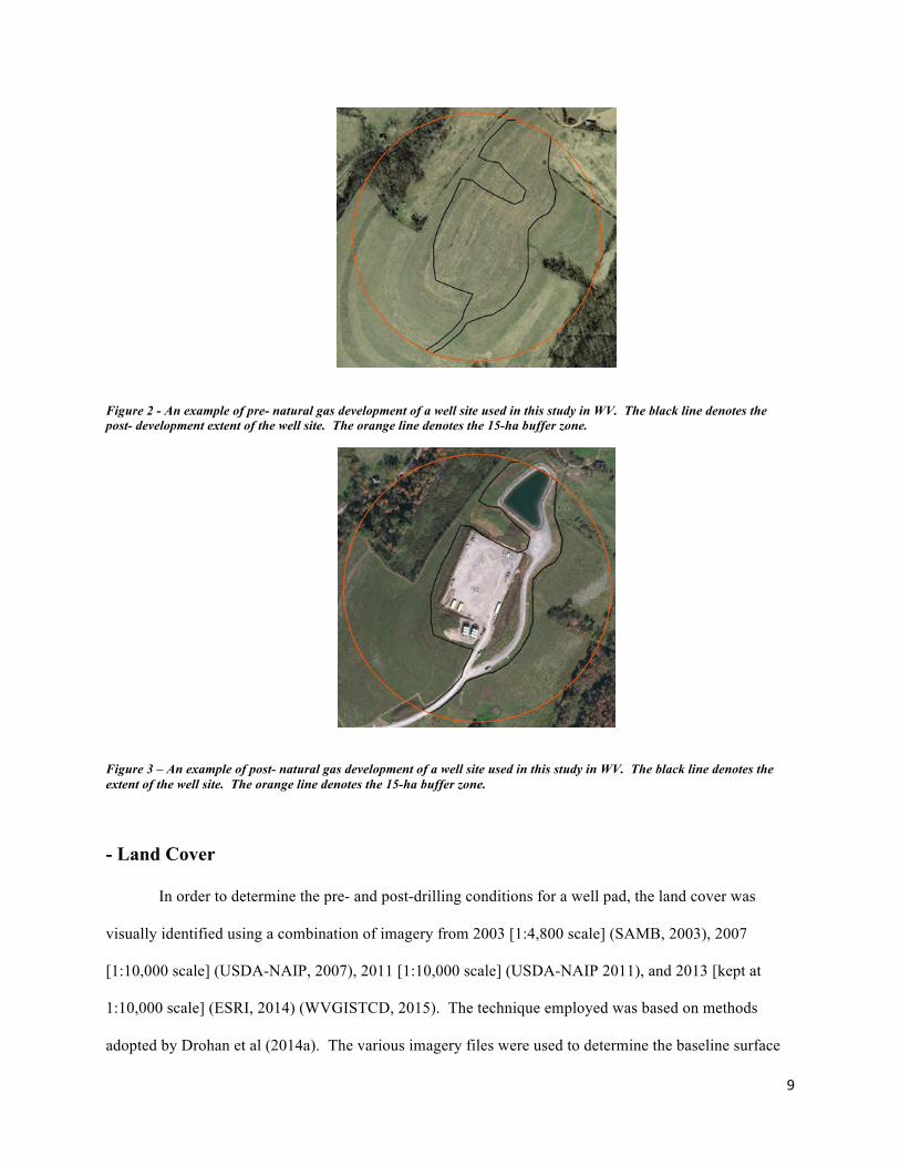
within the buffered area. Examples of pre- and post- natural gas development can be observed in Figure 2
and Figure 3.
9
Figure 2 - An example of pre- natural gas development of a well site used in this study in WV. The black line denotes the post- development extent of the well site. The orange line denotes the 15-ha buffer zone.
Figure 3 – An example of post- natural gas development of a well site used in this study in WV. The black line denotes the extent of the well site. The orange line denotes the 15-ha buffer zone.
- Land Cover
In order to determine the pre- and post-drilling conditions for a well pad, the land cover was
visually identified using a combination of imagery from 2003 [1:4,800 scale] (SAMB, 2003), 2007
[1:10,000 scale] (USDA-NAIP, 2007), 2011 [1:10,000 scale] (USDA-NAIP 2011), and 2013 [kept at
1:10,000 scale] (ESRI, 2014) (WVGISTCD, 2015). The technique employed was based on methods
adopted by Drohan et al (2014a). The various imagery files were used to determine the baseline surface
10
conditions for a well prior to natural gas development, and then the surface conditions after natural gas
development had taken place. For example, a well developed in 2010 would use the 2003 and 2007
imagery files to determine the surface conditions pre-development and the 2011 and 2013 imagery files to
determine the surface conditions post-development. The imagery for both C and UC wells were kept at a
set scale of 1:10,000 during any digitization.
The analysis involved the addition and removal of various temporal images for each well site, and
then the observation of any surface change. Pre-drilling conditions were recognized for each well after
selecting the imagery where there was no evidence of gas development within each 15-ha buffer. After
pre-drilling conditions were established for each well, the post-drilling imagery and conditions were
obtained using a comparable approach. The extent of surface disturbance within each 15-ha buffer,
around the time drilling had occurred, was determined and used for the post-development imagery.
After the best and most appropriate pre- and post-imagery had been selected for each well
through visual inspection, the extent of disturbance was digitized within each 15-ha buffer by overlaying
the well locations and post-drilling imagery. The extent of disturbance area for each well was then
subdivided and digitized by disturbance type, e.g., roads, pads, ponds, and pipelines. The methods
employed for digitizing were the same for both C and UC gas development types.
Forest cover was determined by overlaying the well locations and extent of disturbance with the
pre-drilling imagery and then heads-up digitizing all forest cover within each extent of disturbance.
Heads-up digitizing involves using a drawing tool to digitize a shapefile, over a map, within a GIS
environment. Areas within each zone were either deemed forested or non-forested with each being
digitized into its own coverage type.
- ELUs
Ecological land unit (ELU) models were used to quantify the landscape characteristics within the
overall disturbance for each well. The ELUs were formulated by creating a composite of landforms,
11
geology, soils, and elevation. The ELUs are categorized into the following classes: cliff, steep slope,
slope crest, upper slope, flat summit, sideslope, cove, dry flat, moist flat, wet flat, and slope bottom. The
various categories are based on their location as different landforms in regards to elevation, slope, and soil
type. These landforms can give rise to specific ecological land classifications, and so they’re used to
estimate biodiversity (McNab, 1992). The ELU information was created by the Natural Resource
Analysis Center at WVU and the dataset was downloaded from the WV GIS technical center
(WVGISTCD, 2015). The elevation data used for the ELU model originated from a digital elevation
model (DEM) created by the 2003 WV SAMB, which had a resolution of 3 m. The ELU model used a
final resolution of 9 m.
- Forest Cover
To gain better insight into the characteristics of the forest cover impacts during development,
Forest Inventory and Analysis (FIA) data were downloaded for each county represented within the
drilling regions of this study. The US Forest Service collects FIA data at the county level across the
country. FIA data are gathered to act as a census of US forests and are used to determine if the present
management practices are sustainable long term, how well policies are working to maintain forests for the
next generations, and gauge how the forests will appear in 10 to 50 years. The FIA data are stored in an
online database and can be manipulated using Forest Inventory Data Online (FIDO). Using the FIDO
(2012), volume (board feet)/biomass (short tons) and area data can be selected for a given region/county.
The following dataset types from 2012 were selected and downloaded using FIDO:
• Biomass (BM) - All live tree and sapling aboveground biomass on forest land, oven-dry, by
species group and diameter class (in short tons, equal to 2000 lbs.)
• Volume - All live gross sawtimber volume on forest land by species group and diameter class (in
board feet [BF], equal to 1 ft x 1 ft x 1 in)
• Acreage - Area of forest land by forest type group and ownership group (in acres)
12
The data were then compiled and summarized into a database for further analysis, and then used
to determine biomass per acre and volume per acre for each county. The biomass per acre and volume
per acre for each county were calculated by dividing the total county volume (biomass) by the total
forestland acreage. These values were then recorded, assembled, and converted to ha into a database for
each county. The volume data was converted from BF to cubic meters (CM). This information was used
as part of the process to estimate, on average at the county level, the composition of the forest areas that
was removed, and the value of the associated timber.
The comparison and analysis of the differences between C and UC gas development methods
were based on the various surface impacts and their related areas. The surface impacts were observed,
recorded, and analyzed in a GIS environment. Using a combination of these analyses, the various surface
impacts for C and UC gas development methods were determined and their associated ha were then
recorded. The FIA county-level database was then used to determine the forest volume per ha and
biomass per ha.
- Forest Fragmentation
A preassembled forest fragmentation GIS layer (Strager and Maxwell, 2012) was used to
determine the extent of what was impacted from the C and UC wells of this study. The forest
fragmentation GIS layer was generated using 2011 forest cover conditions. The layer was created using a
9m land cover dataset. The dataset was reclassified into forest and non-forest areas, using a 15-pixel
aggregation input. This allowed for the areas of less than 15 pixels of contiguous area to be absorbed by
its surrounding layer class, which was used to remove small canopy gaps and breaks in the dataset. The
subsequent dataset was then analyzed using morphological image processing, which uses mathematical
morphology to determine the shape and form of objects and areas (Strager and Maxwell, 2012) (Soille,
2003). The forest fragmentation classifications (core, patch, perforated, and edge) were similar to those
described in Vogt et al. (2007). The final forest fragmentation layer was classified into six different
13
types, with no-data relating to non-forested areas: patch, edge, perforated, core (<101.17 ha), core
(101.17-202.34 ha), and core (>202.34 ha).
Since the forest fragmentation layer was developed using 2011 data, many of the C and UC wells
sampled in this project were already represented as completely non-forested area. Wells with preexisting
gaps were removed from the analysis because they did not provide any insight about what forest
fragmentation type existed prior to development.
A statewide subsample of 58 C wells, taken from the 296 C wells, and 52 UC wells, taken from
the 191 UC wells, remained after removing those wells that were already identified as gaps in the
fragmentation layer. Using ArcGIS, the forest fragmentation classification layer was laid over the
subsample wells’ overall disturbed area shapefiles. The classifications within the shapefiles were
tabulated and summed for analysis.
- Natural Gas Production
In order to develop metrics for natural gas production and surface disturbance, production
information was acquired for each well included in the study. Operators are required by state law to
report their production information. According to WV Legislative Rules Title 35 Series 4 section 15.1
and Title 35 Series 8 Section 11 (WVDEP-OOG 2010), “an annual report of oil, gas, and natural gas
liquids production shall be filed with the Chief of the Office of Oil and Gas on or before the succeeding
March 31st.” The reports contain information about the operator and the monthly amount of oil and gas
produced over the course of the prior calendar year. The WVDEP Office of Oil and Gas controls the
production data and manages its disbursement.
The production data were downloaded from the WVDEP website for the years 2009 - 2012 and
matched to those wells included in the analyses using a unique identifier termed the American Petroleum
Institute (API) number. Data downloaded from the WVDEP included the individualized code for each
well, the name of the operator, and information about each well’s monthly gas and oil production. The oil
14
and gas operators for each well report their own data to the WVDEP Office of Oil and Gas once per
calendar year.
A metric was then generated to determine how the alternative drilling methods differ in their gas
production per unit of disturbed area. Even though most UC wells have a production success rate of
nearly 100%, well production can vary. Also, most of these wells show a rapid decline in their
production after the first year of operations. To properly characterize how much gas is being produced
per unit of area disturbed, the production values needed to be weighted by their time in production.
Therefore, production was scaled by taking the total amount of gas produced, in MCF, for the months the
well produced gas during the 2009 - 2012 time period and dividing it by the total number of months. The
values were then divided by the disturbed area, yielding the metric.
- Analyses
Normality assumptions for total disturbed area were tested using the Shapiro-Wilk test statistic
for individual well types as well as aggregated data. Data collected for the total disturbed area were
normal for C wells but were positively skewed for UC wells. This was due to a limited number of
samples that had extremely large impacts on surface parcels. Since the aggregated data did not meet
normality assumptions (P<0.0001), and the extreme observations were not considered outliers, non-
parametric statistical methods were used. The Wilcoxon rank-sum method was used to test for
differences in the total disturbed area between C and UC wells. Further, Spearman’s rank correlation was
used to measure the statistical dependence between the total disturbed area and the year the well was
originally spudded. These non-parametric tests were also used for both the forested area and production
per disturbed area hypothesis tests.
15
Results:
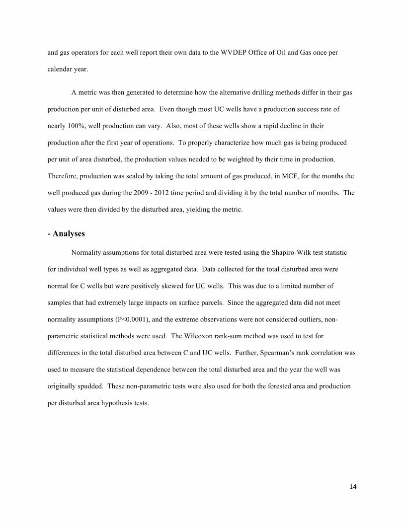
A total of 559 UC wells were spudded during the period of 2009 - 2012 (WVGES, 2014). The
number of wells increased rapidly between 2009 and 2011, then declined in 2012 (Figure 4). The
majority of the UC wells were drilled with the purpose of producing natural gas (79%) or natural gas and
oil (21%). Only three UC wells drilled during this period were recorded as dry.
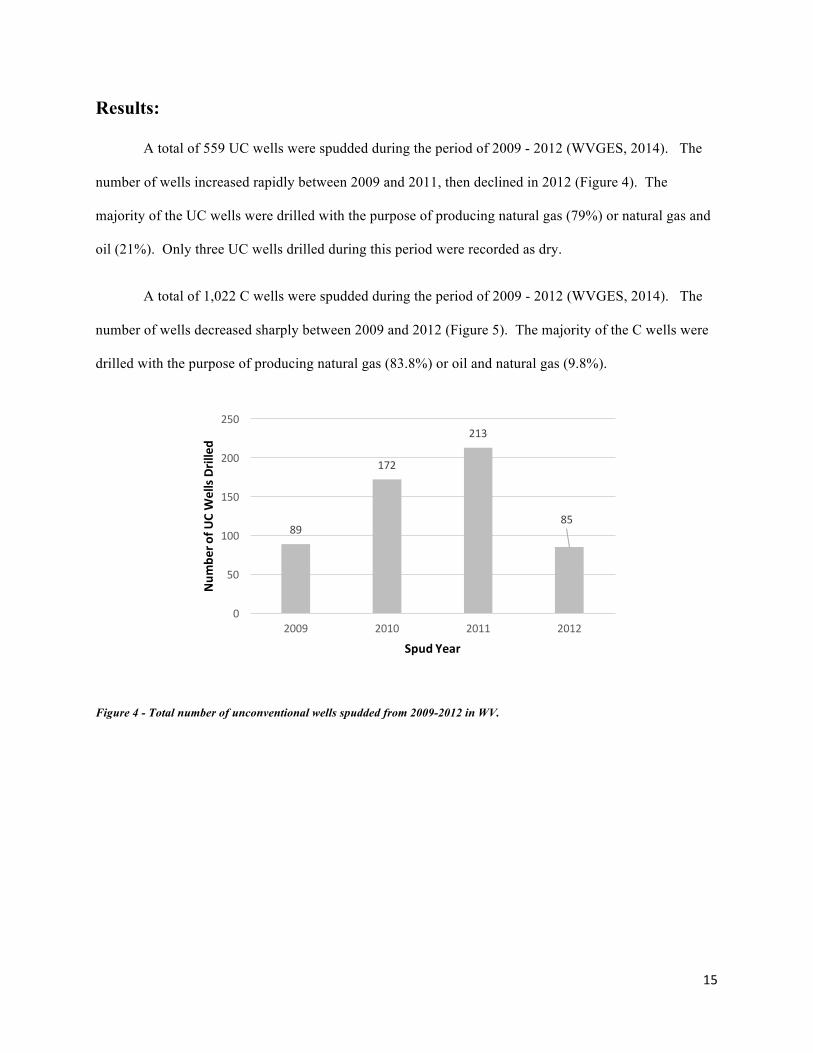
A total of 1,022 C wells were spudded during the period of 2009 - 2012 (WVGES, 2014). The
number of wells decreased sharply between 2009 and 2012 (Figure 5). The majority of the C wells were
drilled with the purpose of producing natural gas (83.8%) or oil and natural gas (9.8%).
Figure 4 - Total number of unconventional wells spudded from 2009-2012 in WV.
89
172
213
85
0
50
100
150
200
250
2009 2010 2011 2012
Num
bero
fUCWellsDrilled
SpudYear
16
Figure 5 - Total number of conventional wells spudded from 2009-2012 in WV.
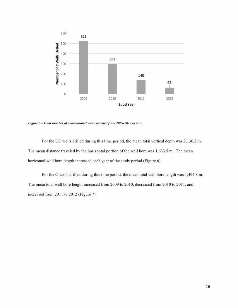
For the UC wells drilled during this time period, the mean total vertical depth was 2,136.2 m.
The mean distance traveled by the horizontal portion of the well bore was 1,633.5 m. The mean
horizontal well bore length increased each year of the study period (Figure 6).
For the C wells drilled during this time period, the mean total well bore length was 1,494.8 m.
The mean total well bore length increased from 2009 to 2010, decreased from 2010 to 2011, and
increased from 2011 to 2012 (Figure 7).
525
295
140
62
0
100
200
300
400
500
600
2009 2010 2011 2012
Num
bero
fCW
ellsDrilled
SpudYear
17
Figure 6 - Mean horizontal well bore length for unconventional gas wells spudded from 2009-2012 in WV (WVGES, 2014).
Figure 7 - Mean total well bore length conventional gas wells spudded from 2009-2012 in WV (WVGES, 2014).
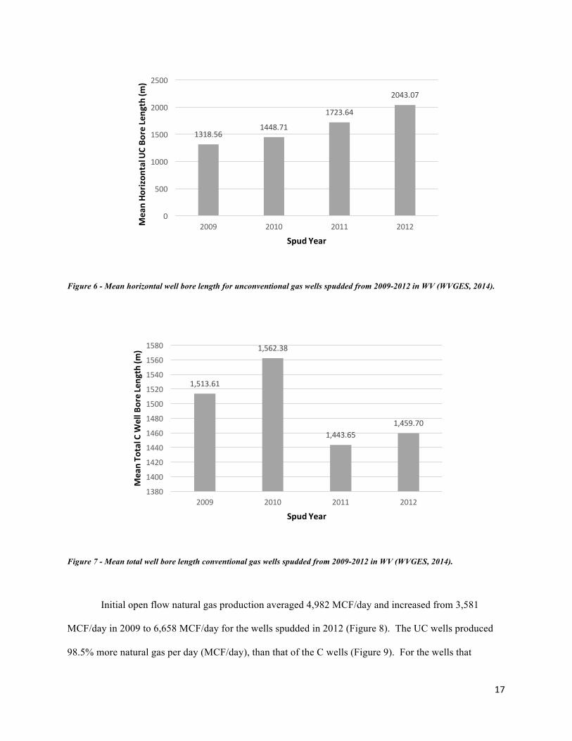
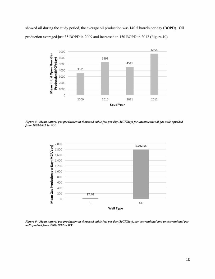
Initial open flow natural gas production averaged 4,982 MCF/day and increased from 3,581
MCF/day in 2009 to 6,658 MCF/day for the wells spudded in 2012 (Figure 8). The UC wells produced
98.5% more natural gas per day (MCF/day), than that of the C wells (Figure 9). For the wells that
1318.561448.71
1723.64
2043.07
0
500
1000
1500
2000
2500
2009 2010 2011 2012MeanHo
rizon
talU
CBo
reLe
ngth(m
)
SpudYear
1,513.61
1,562.38
1,443.651,459.70
1380
1400
1420
1440
1460
1480
1500
1520
1540
1560
1580
2009 2010 2011 2012
MeanTo
talCW
ellB
oreLeng
th(m
)
SpudYear
18
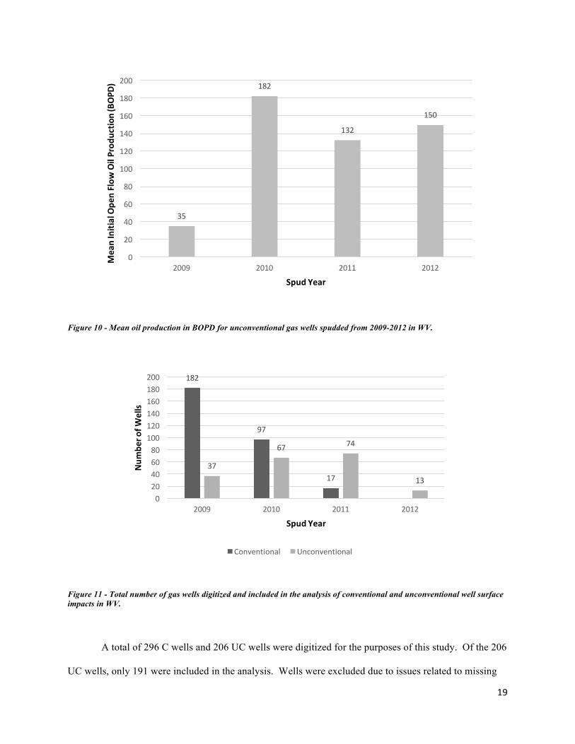
showed oil during the study period, the average oil production was 140.5 barrels per day (BOPD). Oil
production averaged just 35 BOPD in 2009 and increased to 150 BOPD in 2012 (Figure 10).
Figure 8 - Mean natural gas production in thousand cubic feet per day (MCF/day) for unconventional gas wells spudded from 2009-2012 in WV.
Figure 9 - Mean natural gas production in thousand cubic feet per day (MCF/day), per conventional and unconventional gas well spudded from 2009-2012 in WV.
3581
52914541
6658
0
1000
2000
3000
4000
5000
6000
7000
2009 2010 2011 2012
MeanInitialOpe
nFlow
Gas
Prod
uctio
n(M
CF/day)
SpudYear
27.40
1,792.55
0
200
400
600
800
1,000
1,200
1,400
1,600
1,800
2,000
C UCMeanGa
sProdu
tionpe
rDay(M
CF/day)
WellType
19
Figure 10 - Mean oil production in BOPD for unconventional gas wells spudded from 2009-2012 in WV.
Figure 11 - Total number of gas wells digitized and included in the analysis of conventional and unconventional well surface impacts in WV.
A total of 296 C wells and 206 UC wells were digitized for the purposes of this study. Of the 206
UC wells, only 191 were included in the analysis. Wells were excluded due to issues related to missing
35
182
132
150
0
20
40
60
80
100
120
140
160
180
200
2009 2010 2011 2012
MeanInitialOpe
nFlow
OilProd
uctio
n(BOPD
)
SpudYear
182
97
1737
67 74
13
020406080
100120140160180200
2009 2010 2011 2012
Num
bero
fWells
SpudYear
Conventional Unconventional
20
data (API numbers/permit numbers or locational information) and incorrect data (API numbers/permit
numbers, locational information, or imagery related issues). Some wells were missing or had incorrect
locational information, so the wells could not be found and mapped for analysis. Each well has a unique
associated API number, which is needed to delineate that well from all others. The API number was also
needed to determine production information. Figure 11 displays the number of wells per spud year for
each well type, C and UC. The growth in shale-gas activity from 2009 to 2011 and its increasing share of
overall activity are evident. The lack of C wells and the decline in UC wells in 2012 was due to a
combination of factors, including the sheer number of wells from the previous years, the lack of
completed well data for 2012, and the random selection process of the study.
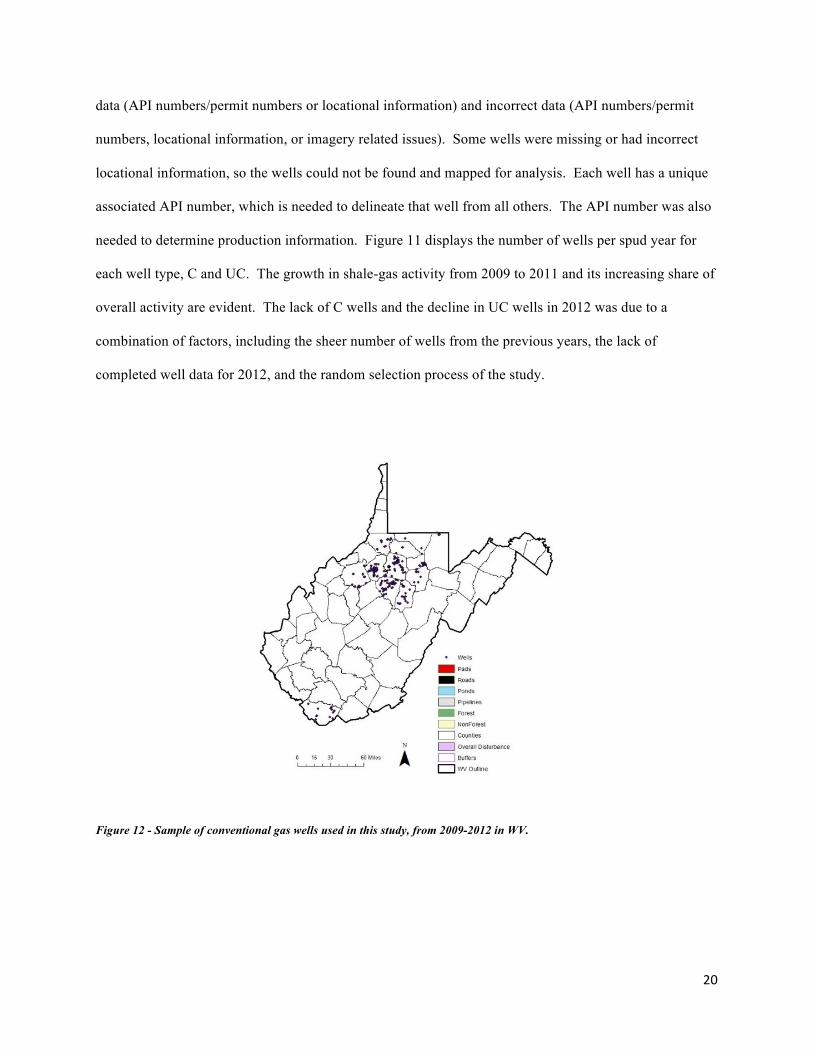
Figure 12 - Sample of conventional gas wells used in this study, from 2009-2012 in WV.
21
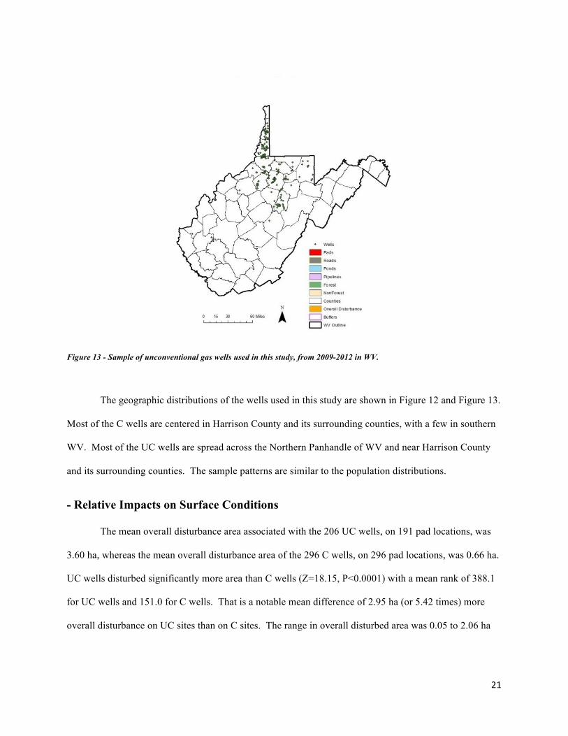
Figure 13 - Sample of unconventional gas wells used in this study, from 2009-2012 in WV.
The geographic distributions of the wells used in this study are shown in Figure 12 and Figure 13.
Most of the C wells are centered in Harrison County and its surrounding counties, with a few in southern
WV. Most of the UC wells are spread across the Northern Panhandle of WV and near Harrison County
and its surrounding counties. The sample patterns are similar to the population distributions.
- Relative Impacts on Surface Conditions
The mean overall disturbance area associated with the 206 UC wells, on 191 pad locations, was
3.60 ha, whereas the mean overall disturbance area of the 296 C wells, on 296 pad locations, was 0.66 ha.
UC wells disturbed significantly more area than C wells (Z=18.15, P<0.0001) with a mean rank of 388.1
for UC wells and 151.0 for C wells. That is a notable mean difference of 2.95 ha (or 5.42 times) more
overall disturbance on UC sites than on C sites. The range in overall disturbed area was 0.05 to 2.06 ha
22
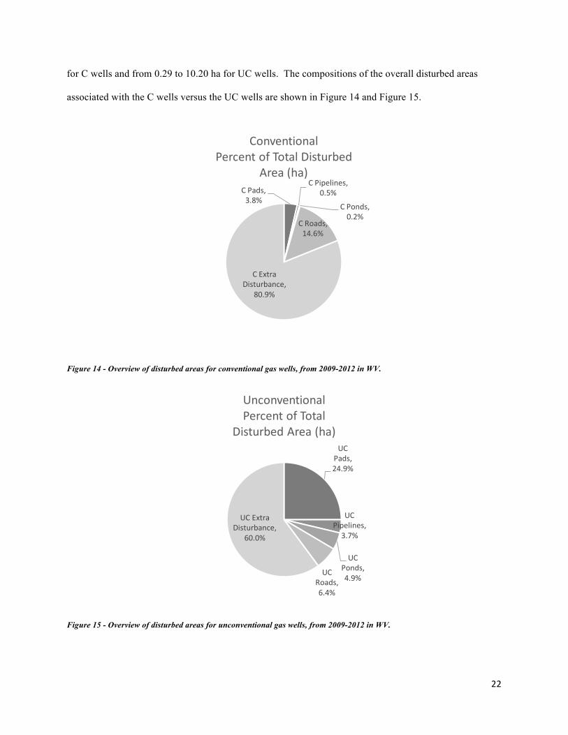
for C wells and from 0.29 to 10.20 ha for UC wells. The compositions of the overall disturbed areas
associated with the C wells versus the UC wells are shown in Figure 14 and Figure 15.
Figure 14 - Overview of disturbed areas for conventional gas wells, from 2009-2012 in WV.
Figure 15 - Overview of disturbed areas for unconventional gas wells, from 2009-2012 in WV.
CPads,3.8%
CPipelines,0.5%
CPonds,0.2%
CRoads,14.6%
CExtraDisturbance,
80.9%
ConventionalPercentofTotalDisturbed
Area(ha)
UCPads,24.9%
UCPipelines,3.7%
UCPonds,4.9%
UCRoads,6.4%
UCExtraDisturbance,
60.0%
UnconventionalPercentofTotal
DisturbedArea(ha)
23
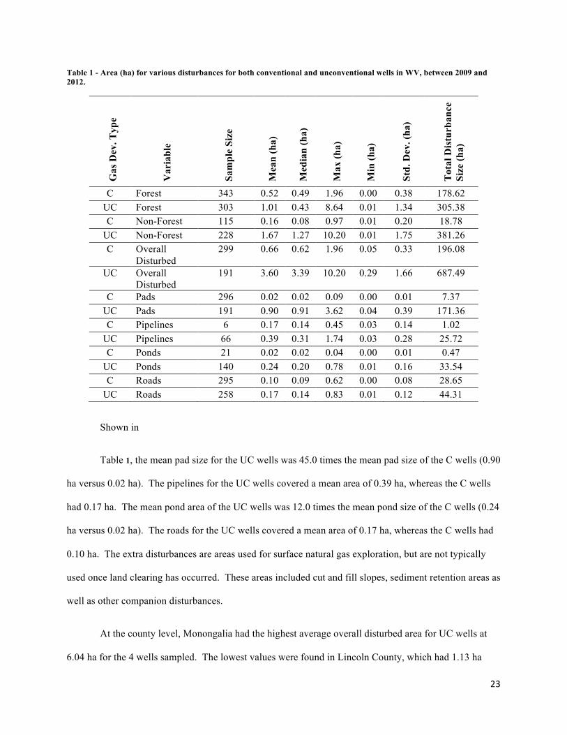
Table 1 - Area (ha) for various disturbances for both conventional and unconventional wells in WV, between 2009 and 2012.
Gas
Dev
. Typ
e
Var
iabl
e
Sam
ple
Size
Mea
n (h
a)
Med
ian
(ha)
Max
(ha)
Min
(ha)
Std.
Dev
. (ha
)
Tot
al D
istu
rban
ce
Size
(ha)
C Forest 343 0.52 0.49 1.96 0.00 0.38 178.62 UC Forest 303 1.01 0.43 8.64 0.01 1.34 305.38 C Non-Forest 115 0.16 0.08 0.97 0.01 0.20 18.78
UC Non-Forest 228 1.67 1.27 10.20 0.01 1.75 381.26 C Overall
Disturbed 299 0.66 0.62 1.96 0.05 0.33 196.08
UC Overall Disturbed
191 3.60 3.39 10.20 0.29 1.66 687.49
C Pads 296 0.02 0.02 0.09 0.00 0.01 7.37 UC Pads 191 0.90 0.91 3.62 0.04 0.39 171.36 C Pipelines 6 0.17 0.14 0.45 0.03 0.14 1.02
UC Pipelines 66 0.39 0.31 1.74 0.03 0.28 25.72 C Ponds 21 0.02 0.02 0.04 0.00 0.01 0.47
UC Ponds 140 0.24 0.20 0.78 0.01 0.16 33.54 C Roads 295 0.10 0.09 0.62 0.00 0.08 28.65
UC Roads 258 0.17 0.14 0.83 0.01 0.12 44.31
Shown in
Table 1, the mean pad size for the UC wells was 45.0 times the mean pad size of the C wells (0.90
ha versus 0.02 ha). The pipelines for the UC wells covered a mean area of 0.39 ha, whereas the C wells
had 0.17 ha. The mean pond area of the UC wells was 12.0 times the mean pond size of the C wells (0.24
ha versus 0.02 ha). The roads for the UC wells covered a mean area of 0.17 ha, whereas the C wells had
0.10 ha. The extra disturbances are areas used for surface natural gas exploration, but are not typically
used once land clearing has occurred. These areas included cut and fill slopes, sediment retention areas as
well as other companion disturbances.
At the county level, Monongalia had the highest average overall disturbed area for UC wells at
6.04 ha for the 4 wells sampled. The lowest values were found in Lincoln County, which had 1.13 ha
24
disturbed for its single well. Barbour County had the highest overall disturbed area for C wells at 0.89 ha
for the 8 wells sampled. Preston County had the lowest values for C wells, with an average of 0.45 ha
disturbed across 9 wells. There was no relationship between the total disturbed area and the year the well
was spudded for UC wells (r=0.06000, P=0.2980) and C wells (r=0.12941, p=0.0744). Likewise, there
was no relationship between total disturbed area and drilling year (r=0.06070, p=0.2980).
The 296 pads for the 296 C wells had a minimum area of less than 0.01 ha and a maximum pad
area of 0.09 ha. The 191 pads for the 206 UC wells had a minimum area of 0.04 ha and a maximum pad
area of 3.62 ha. This indicates that the UC wells have much larger pads (and also disturbed areas),
compared to the C wells. The UC wells have a mean of 0.90 ha of pad area compared to the C wells
mean of 0.03 ha of pad area.
Pad areas represent 24.9% of the mean overall disturbance for UC wells and just 3.8% of the
mean overall disturbance for C wells. Therefore, pads on UC sites utilize a greater share of the overall
disturbed area than do pads on C sites.
The mean disturbed forested area for the C wells was 0.52 ha, with a standard deviation of 0.38.
The mean disturbed forested area for the UC wells was 1.01 ha, with a standard deviation of 1.34. The
UC mean disturbed forest area was nearly twice the size of the C mean disturbed forest area.
With respect to hypothesis testing, both H1(a)0 and H1(b)0 were rejected and the corresponding
alternative hypotheses, H1(a)a and H1(b)a, were adopted. That is, UC wells had both a greater total
disturbed area and a mean disturbed forest area than C wells.
C wells had a significantly greater portion of their disturbed area before development in forest
cover versus UC wells (Z =-13.55, P<0.0001). The mean rank score for C wells was 310.9 versus 139.3
for UC wells. There was no relationship in the proportion of disturbed area in forest and spud year for C
wells; however, there was a relationship found for UC wells. It was found that as spud year increased
25
from 2009 through 2012, the amount of forest cover in the disturbed area decreased (r=-0.15781,
p=0.0292).
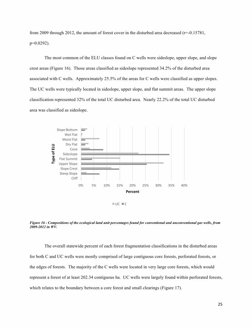
The most common of the ELU classes found on C wells were sideslope, upper slope, and slope
crest areas (Figure 16). Those areas classified as sideslope represented 34.2% of the disturbed area
associated with C wells. Approximately 25.5% of the areas for C wells were classified as upper slopes.
The UC wells were typically located in sideslope, upper slope, and flat summit areas. The upper slope
classification represented 32% of the total UC disturbed area. Nearly 22.2% of the total UC disturbed
area was classified as sideslope.
Figure 16 - Compositions of the ecological land unit percentages found for conventional and unconventional gas wells, from 2009-2012 in WV.
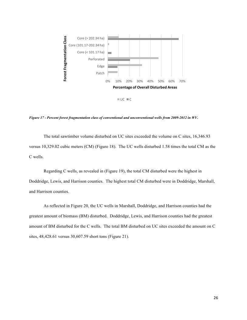
The overall statewide percent of each forest fragmentation classifications in the disturbed areas
for both C and UC wells were mostly comprised of large contiguous core forests, perforated forests, or
the edges of forests. The majority of the C wells were located in very large core forests, which would
represent a forest of at least 202.34 contiguous ha. UC wells were largely found within perforated forests,
which relates to the boundary between a core forest and small clearings (Figure 17).
0% 5% 10% 15% 20% 25% 30% 35% 40%
CliffSteepSlopeSlopeCrestUpperSlopeFlatSummitSideslope
CoveDryFlat
MoistFlatWetFlat
SlopeBottom
Percent
Type
ofELU
UC C
26
Figure 17 - Percent forest fragmentation class of conventional and unconventional wells from 2009-2012 in WV.
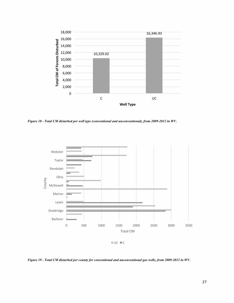
The total sawtimber volume disturbed on UC sites exceeded the volume on C sites, 16,346.93
versus 10,329.02 cubic meters (CM) (Figure 18). The UC wells disturbed 1.58 times the total CM as the
C wells.
Regarding C wells, as revealed in (Figure 19), the total CM disturbed were the highest in
Doddridge, Lewis, and Harrison counties. The highest total CM disturbed were in Doddridge, Marshall,
and Harrison counties.
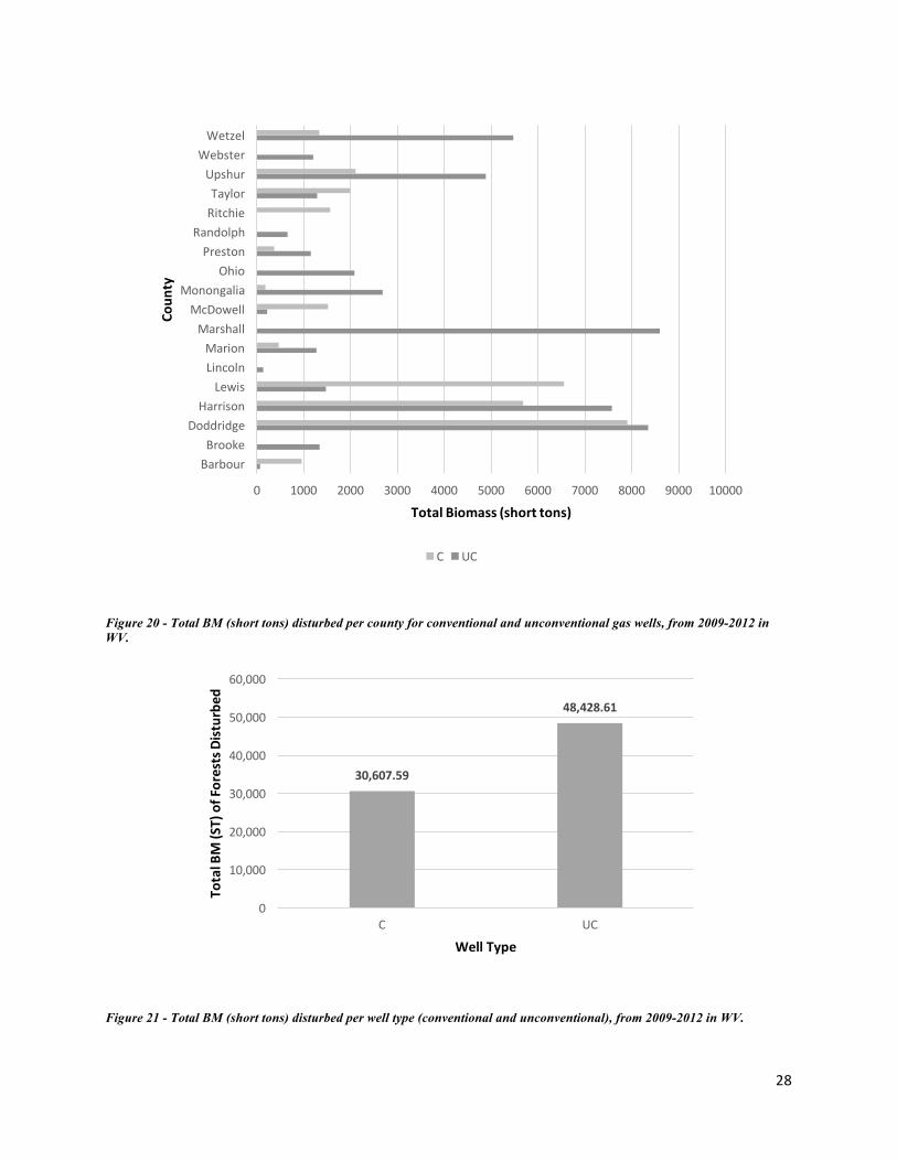
As reflected in Figure 20, the UC wells in Marshall, Doddridge, and Harrison counties had the
greatest amount of biomass (BM) disturbed. Doddridge, Lewis, and Harrison counties had the greatest
amount of BM disturbed for the C wells. The total BM disturbed on UC sites exceeded the amount on C
sites, 48,428.61 versus 30,607.59 short tons (Figure 21).
0% 10% 20% 30% 40% 50% 60% 70%
Patch
Edge
Perforated
Core(<101.17ha)
Core(101.17-202.34ha)
Core(>202.34ha)
PercentageofOverallDisturbedAreas
ForestFragmen
tatio
nClass
UC C
27
Figure 18 - Total CM disturbed per well type (conventional and unconventional), from 2009-2012 in WV.
Figure 19 - Total CM disturbed per county for conventional and unconventional gas wells, from 2009-2012 in WV.
10,329.02
16,346.93
0
2,000
4,000
6,000
8,000
10,000
12,000
14,000
16,000
18,000
C UC
TotalCMofForestsDisturbe
d
WellType
0 500 1000 1500 2000 2500 3000 3500
Barbour
Doddridge
Lewis
Marion
McDowell
Ohio
Randolph
Taylor
Webster
TotalCM
Coun
ty
UC C
28
Figure 20 - Total BM (short tons) disturbed per county for conventional and unconventional gas wells, from 2009-2012 in WV.
Figure 21 - Total BM (short tons) disturbed per well type (conventional and unconventional), from 2009-2012 in WV.
0 1000 2000 3000 4000 5000 6000 7000 8000 9000 10000
BarbourBrooke
DoddridgeHarrison
LewisLincolnMarion
MarshallMcDowell
MonongaliaOhio
PrestonRandolph
RitchieTaylorUpshur
WebsterWetzel
TotalBiomass(shorttons)
Coun
ty
C UC
30,607.59
48,428.61
0
10,000
20,000
30,000
40,000
50,000
60,000
C UC
TotalBM(ST)ofForestsDisturbe
d
WellType
29
The estimated values of the forests disturbed during gas development for C and UC wells were
determined using per-MBF stumpage prices found in the West Virginia University Appalachian
Hardwood Center quarterly stumpage price report from December 2012 (AHC, 2015). The regional
stumpage data was converted into county level information. The BM and CM values were determined for
each county. The site specific total disturbed forest area data for the C and UC wells were then used to
calculate and quantify the overall disturbed forest valuations.
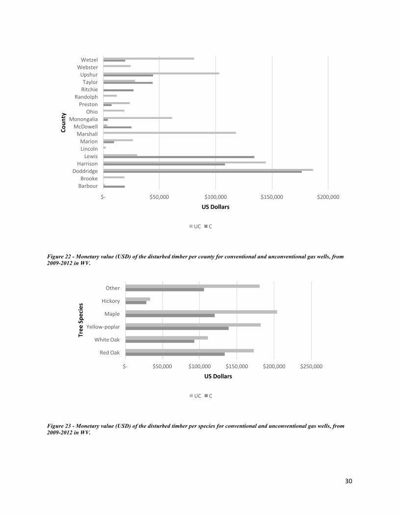
Figure 22 shows the value of the timber removed during gas development for C and UC wells for
each county represented in the study. Figure 23 offers insight into the values of the disturbed timber
decomposed by the species on both C and UC sites. Yellow-poplar represented the highest share of the
value of timber disturbed on C sites ($138,801), while maple accounted for the greatest share of the value
of timber disturbed on UC sites ($203,937). The timber disturbed on C sites had a total value of
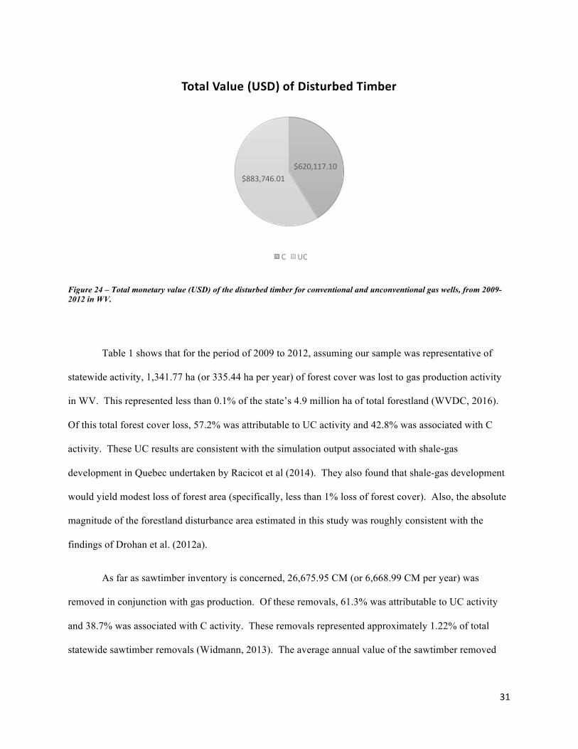
$620,117, while the timber disturbed on UC wells had a total value of $883,746 (Figure 24). This yielded
an overall value of $1,503,863 with respect to timber disturbed for the period of 2009-2012.
30
Figure 22 - Monetary value (USD) of the disturbed timber per county for conventional and unconventional gas wells, from 2009-2012 in WV.
Figure 23 - Monetary value (USD) of the disturbed timber per species for conventional and unconventional gas wells, from 2009-2012 in WV.
$- $50,000 $100,000 $150,000 $200,000
BarbourBrooke
DoddridgeHarrison
LewisLincolnMarion
MarshallMcDowell
MonongaliaOhio
PrestonRandolph
RitchieTaylorUpshur
WebsterWetzel
USDollars
Coun
ty
UC C
$- $50,000 $100,000 $150,000 $200,000 $250,000
RedOak
WhiteOak
Yellow-poplar
Maple
Hickory
Other
USDollars
TreeSpe
cies
UC C
31
Figure 24 – Total monetary value (USD) of the disturbed timber for conventional and unconventional gas wells, from 2009-2012 in WV.
Table 1 shows that for the period of 2009 to 2012, assuming our sample was representative of
statewide activity, 1,341.77 ha (or 335.44 ha per year) of forest cover was lost to gas production activity
in WV. This represented less than 0.1% of the state’s 4.9 million ha of total forestland (WVDC, 2016).
Of this total forest cover loss, 57.2% was attributable to UC activity and 42.8% was associated with C
activity. These UC results are consistent with the simulation output associated with shale-gas
development in Quebec undertaken by Racicot et al (2014). They also found that shale-gas development
would yield modest loss of forest area (specifically, less than 1% loss of forest cover). Also, the absolute
magnitude of the forestland disturbance area estimated in this study was roughly consistent with the
findings of Drohan et al. (2012a).
As far as sawtimber inventory is concerned, 26,675.95 CM (or 6,668.99 CM per year) was
removed in conjunction with gas production. Of these removals, 61.3% was attributable to UC activity
and 38.7% was associated with C activity. These removals represented approximately 1.22% of total
statewide sawtimber removals (Widmann, 2013). The average annual value of the sawtimber removed
$620,117.10$883,746.01
TotalValue(USD)ofDisturbedTimber
C UC
32
was $375,966. There can be limitations using county-level resolution FIA data. The resolution is not at a
site specific level, so there could be some discrepancy using the county-level resolution as an estimate.
A general tendency regarding ELUs was that most wells were not located in flat areas. This
could be due to a combination of factors, including, the natural topography of the state of WV, the below-
ground conditions affecting gas development site establishment on flat areas, and the geographic
distribution of the shale (most prevalent in the Appalachian plateau and ridge-valley areas) (Enomoto et
al., 2012).
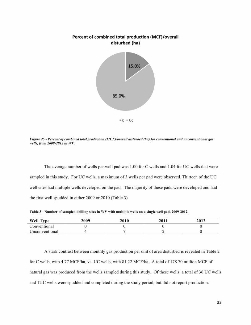
- Relative Gas Production per Unit of Area Disturbed
The production data were incorporated into SAS software and analyzed for the previously
specified metrics. As shown in Table 2, the C wells had a total overall disturbance area of 196.66 ha,
whereas the UC wells had more than three times that amount, or 687.49 ha. The total production values
for the C and UC wells were 8,542,345 MCF and 170,148,007 MCF, respectively. The C wells
represented only 15% of the combined production per overall disturbed area in the study. UC wells
demonstrated much greater productivity, with approximately 85% of the combined total production per
unit of disturbed area (Figure 25).
Table 2 - Production and calculated metrics for conventional and unconventional gas wells, from 2009-2012 in WV.
Wel
l Typ
e
Ove
rall
Dis
turb
ance
(ha)
Tot
al P
rodu
ctio
n (M
CF)
Mon
ths o
f Pr
oduc
tion
Tot
al P
rodu
ctio
n/
Mon
th (M
CF)
Tot
al P
rodu
ctio
n (M
CF)
/Mon
th/
Ove
rall
Dis
turb
ed (h
a)
Tot
al P
rodu
ctio
n (M
CF)
/Ove
rall
Dis
turb
ed (h
a)
C 196.66 8,542,345.00 9,102.00 938.51 4.77 43,436.90 UC 687.49 170,148,007.00 3,047.00 55,841.16 81.22 247,492.31
33
Figure 25 - Percent of combined total production (MCF)/overall disturbed (ha) for conventional and unconventional gas wells, from 2009-2012 in WV.
The average number of wells per well pad was 1.00 for C wells and 1.04 for UC wells that were
sampled in this study. For UC wells, a maximum of 3 wells per pad were observed. Thirteen of the UC
well sites had multiple wells developed on the pad. The majority of these pads were developed and had
the first well spudded in either 2009 or 2010 (Table 3).
Table 3 - Number of sampled drilling sites in WV with multiple wells on a single well pad, 2009-2012.
Well Type 2009 2010 2011 2012 Conventional 0 0 0 0 Unconventional 4 7 2 0
A stark contrast between monthly gas production per unit of area disturbed is revealed in Table 2
for C wells, with 4.77 MCF/ha, vs. UC wells, with 81.22 MCF/ha. A total of 178.70 million MCF of
natural gas was produced from the wells sampled during this study. Of these wells, a total of 36 UC wells
and 12 C wells were spudded and completed during the study period, but did not report production.
15.0%
85.0%
Percentofcombinedtotalproduction(MCF)/overalldisturbed(ha)
C UC
34
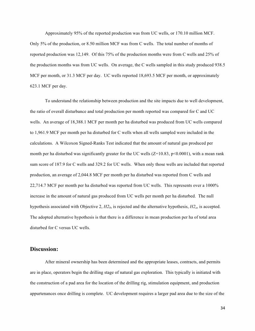
Approximately 95% of the reported production was from UC wells, or 170.10 million MCF.
Only 5% of the production, or 8.50 million MCF was from C wells. The total number of months of
reported production was 12,149. Of this 75% of the production months were from C wells and 25% of
the production months was from UC wells. On average, the C wells sampled in this study produced 938.5
MCF per month, or 31.3 MCF per day. UC wells reported 18,693.5 MCF per month, or approximately
623.1 MCF per day.
To understand the relationship between production and the site impacts due to well development,
the ratio of overall disturbance and total production per month reported was compared for C and UC
wells. An average of 18,388.1 MCF per month per ha disturbed was produced from UC wells compared
to 1,961.9 MCF per month per ha disturbed for C wells when all wells sampled were included in the
calculations. A Wilcoxon Signed-Ranks Test indicated that the amount of natural gas produced per
month per ha disturbed was significantly greater for the UC wells (Z=10.83, p<0.0001), with a mean rank
sum score of 187.9 for C wells and 329.2 for UC wells. When only those wells are included that reported
production, an average of 2,044.8 MCF per month per ha disturbed was reported from C wells and
22,714.7 MCF per month per ha disturbed was reported from UC wells. This represents over a 1000%
increase in the amount of natural gas produced from UC wells per month per ha disturbed. The null
hypothesis associated with Objective 2, H20, is rejected and the alternative hypothesis, H2a, is accepted.
The adopted alternative hypothesis is that there is a difference in mean production per ha of total area
disturbed for C versus UC wells.
Discussion:
After mineral ownership has been determined and the appropriate leases, contracts, and permits
are in place, operators begin the drilling stage of natural gas exploration. This typically is initiated with
the construction of a pad area for the location of the drilling rig, stimulation equipment, and production
appurtenances once drilling is complete. UC development requires a larger pad area due to the size of the
35
drilling rigs needed as well as the equipment needed during well stimulation. In order to build a level
drilling location in the mountainous terrain of WV, a larger area must be disturbed to account for the fill
and cut slope areas needed to develop the pad. As part of this overall disturbance, operators must also
have a large road to the pad area to handle the large volumes of truck traffic as well as water
impoundments so that water can be supplied for well stimulation. Once the well is completed and
production starts, gathering lines must also be developed to transport natural gas from the well site to the
closest transmission lines. An objective of this research was to determine and quantify the relative
impacts of C and UC gas development on surface conditions in WV. This development includes the
overall area disturbed by the exploration process as well as portion of this area that can be attributed to
the well pad, road network, water holding structures, and natural gas pipelines.
With more intensive infrastructure (more equipment, larger footprints, etc.) and the possibility for
multiple wells per pad, one would expect the mean total disturbance area associated with UC wells to be
greater than the comparable area associated with C wells. The results found in conjunction with
Hypotheses 1(a) and 1(b) were consistent with this expectation. With respect to Hypothesis H2, the
results indicated that the volume of gas production per unit of area disturbed was much greater for UC
wells than C wells. As time has passed, more and more wells have been drilled per UC pad area in WV,
which is due to advancements in technology and a further understanding of other targeted formations.
The potential for greater production per UC well and the possibility of multiple UC wells per pad (Drohan
et al., 2012a) outweighed the greater surface disturbance associated with UC wells. Thus, public policies
and regulations limiting the expansion of UC wells could have negative consequences associated with the
surface impacts during energy development activities. Although we found that there was not a
relationship between overall disturbed area and year (2009-2012) or in the gas production per ha
disturbed and year, the total acreage of disturbance related to UC development is expected to continue to
get larger with time. Likewise, gas production per unit of disturbed area will continue to increase rapidly
as more wells are added per site. Increased well density on developed pads can benefit both mineral and
36
surface owners through increased production and royalties as well as reduced surface disturbance. As
reported, the average number of wells per well pad was 1.00 for C wells and 1.04 for UC wells that were
sampled. These results support the actual development timeline of UC wells in West Virginia and
surrounding states. It was common in the early years of shale development to drill a single well on a pad
and then move to additional sites to secure acreage. As the play progressed we have started seeing the
drilling rigs stay on an individual pad and continue drilling multiple wells. In this case we did not see
more multiple wells in the 2011 and 2012 data because of the time-lag between the drilling of multiple
wells on a pad.
As far as the source of disturbance is concerned, the findings suggest a marked difference between
UC and C wells. With UC wells and ignoring the “other category” of disturbed area, pads
overwhelmingly represented the major land use in the disturbed area. In contrast, a comparable analysis
in conjunction with C wells indicates that roads were the major land use within the disturbed area. With
C wells, pad sizes do not need to be as large as those used for UC wells.
The relative environmental and ecological impacts of alternative gas production approaches are
not limited to absolute areas disturbed. Drohan et al. (2012b) reported that the roads and pipelines needed
for new gas wells would fragment forest cover and potentially impact runoff into streams, rivers, and
other bodies of water. Furthermore, roads can facilitate the spread of invasive species (Mortensen et al.,
2009) and can negatively influence wildlife habitat (Cushman, 2006). Interestingly, the overlay of C and
UC wells relative to forest fragmentation classification yielded different outcomes.
The C wells were dominated by the core forest fragmentation classification type, whereas the UC
wells’ majority forest fragmentation classification type was perforated. Thus, despite their greater
absolute disturbance footprint, these UC wells may have less relative impact on forest integrity. This
relates to the different relative positioning of the two well types. The UC wells were more likely to be
sited near roadways to reduce the cost of construction of intensive road infrastructure. These results are
37
in contrast to the simulated findings of Racicot et al. (2014), who projected a high degree of disturbance
on core forests in Quebec by UC wells. The empirical findings here were that UC wells were most
frequently on already perforated forests, not on core forests. Thus, the impact on forest fragmentation in
some regions may be less than generally anticipated by some scientists.
Much of the area associated with both C and UC wells was the result of unaccounted for
disturbances, which represents areas that did not fall within any other category. The magnitude of surface
disturbance per pad (3.60 ha) on UC sites was slightly greater than the preliminary estimates of
Grushecky and Wang (2013) (3.0 ha) in WV.
The absolute magnitude of the footprint associated with the disturbed area of WV forestland in
conjunction with four years (2009 to 2012) of gas-production activity was rather modest. An estimated
2,358 hectares were disturbed, of which 1341 hectares were forested. About 73.3% of the estimated
forest area removed was the result of UC production and 26.7% was the result of C production. The total
estimated disturbance of forest due to the natural gas development between 2009 and 2012 represented
less than 0.1% of the state’s forestland. The absolute magnitude of the forestland disturbance area
estimated in this study was roughly consistent with the findings of Drohan et al. (2012a). Interestingly, in
contrast to C wells and studies of UC wells in other regions, the findings for WV suggest that UC wells
were most frequently on already-perforated forests, not on core forests. Thus, the impact on forest
fragmentation in WV may be less than generally anticipated in other regions by some scientists.
In this project, the focus was on the relative loss of forest cover for C versus UC gas wells in WV.
Although UC gas production fared favorably on volume of output per unit of area disturbed, other
variables need to be addressed in future studies. The impact of gas-production methodology on surface
cover and ecological attributes is a complex topic. Refined spatial analysis should be applied to better
assess the impact of gas production approach on forest fragmentation (see, for example, Drohan et al.’s
2012a analysis in Pennsylvania). Another important extension would be the comparison of impacts of

38
alternative gas production systems on CO2 emissions associated with forest loss. Finally, other potentially
negative consequences associated with hydraulic fracking on the local environment—such as methane
contamination of water and hazards associated with both formation chemicals and introduced
chemicals—were not considered in this analysis. More comprehensive ecological analyses of UC activity
in WV will need to incorporate these potential impacts.
39
Bibliography:
Abrahams, L. S., Griffin, W. M., & Matthews, H. S. (2015). Assessment of polices to reduce core forest fragmentation from
Marcellus shale development in Pennsylvania. Ecological Indicators. 52, 153-160.
AHC (2015). WV Timber Market Report. AHC Resources. http://ahc.wvu.edu/ahc-resources-mainmenu-45/timber-market-
report-mainmenu-62
Callahan, J.M. (1923). History of West Virginia, old and new. Chicago, IL: The American Historical Society.
Considine, T. J., Watson, R., & Blumsack, S. (2010). The Economic Impacts of the Pennsylvania Marcellus Shale Natural Gas
Play: An Update. Penn State. 1-77.
http://energy.wilkes.edu/PDFFiles/Library/The%20economic%20impacts%20of%20the%20PA%20marcellus%20shale%20natur
al.pdf
Cruz, J., Smith, P., & Stanley, S. (2014). The Marcellus Shale gas boom in Pennsylvania: employment and wage trends. Mon.
Labor Rev. http://www.bls.gov/opub/mlr/2014/article/the-marcellus-shale-gas-boom-in-pennsylvania.htm
Cushman, S. A. (2006). Effects of habitat loss and fragmentation on amphibians: A review and prospectus. Biological
Conservation, 128(2), 231-240. doi: 10.1016/j.biocon.2005.09.031
Downing, B. (2014). Stone Energy to spud first Utica shale well in West Virginia. Akron Beac. J.
http://www.ohio.com/blogs/drilling/ohio-utica-shale-1.291290/stone-energy-to-spud-first-utica-shale-well-in-west-virginia-
1.486082
Drohan, P. J., Brittingham, M., Bishop, J., & Yoder, K. (2012a). Early Trends in Landcover Change and Forest Fragmentation
Due to Shale-Gas Development in Pennsylvania: A Potential Outcome for the Northcentral Appalachians. Environ. Manage. 49,
1061-1075.
Drohan, P. J., Finley, J. C., Roth, P., Schuler, T. M., Stout, S. L., Brittingham, M.C., & Johnson N. C. (2012b). PERSPECTIVES
FROM THE FIELD: Oil and Gas Impacts on Forest Ecosystems: Findings Gleaned from the 2012 Goddard Forum at Penn State
University. Environ. Pract. 14, 394-6.
Enomoto, C.B., Coleman, Jr. J. L., Haynes, J. T., Whitmeyer, S. J., McDowell, R. R., Lewis, J. E., Spear, T. P., & Swezey, C. S.
(2012). Geology of the Devonian Marcellus Shale—Valley and Ridge province, Virginia and West Virginia—A field trip
guidebook for the American Association of Petroleum Geologists Eastern Section Meeting, September 28–29, 2011: U.S.
40
Geological Survey Open-File Report. 2012-1194, 55 p.
Entrekin, S., Evans-White, M., Johnson, B., & Hagenbuch, E. (2011). Rapid expansion of natural gas development poses a threat
to surface waters. Frontiers in Ecology and the Environment. 9, 503-511.
ESRI (2012). Guerra, Lucy. Now that ArcGIS 10.1 is shipping…. ArcGIS Resource Center Blog. ESRI.
http://blogs.esri.com/esri/arcgis/2012/06/19/now-that-arcgis-10-1-is-shipping/
ESRI (2014). World Imagery.
http://www.arcgis.com/home/item.html?id=10df2279f9684e4a9f6a7f08febac2a9&_ga=1.35432166.612546602.1401725571
FIDO (2014). US Forest Service, FIA Program. Welcome to FIDO!. http://apps.fs.fed.us/fia/fido/index.html
Grushecky, S. T., & Wang, J. (2013). 2013 Council on Forest Engineering Annual Meeting (Missoula, Montana, 2013). 1-8.
Hatzenbuhler, H., & Centner, T. (2012). Regulation of Water Pollution from Hydraulic Fracturing in Horizontally-Drilled Wells
in the Marcellus Shale Region, USA. Water. 4, 983-994.
HBS, & BCG (2015). Innovative Strategy Would Allow U.S. to Capitalize on America’s New Energy Advantage While
Protecting the Environment and Speeding the Transition to a Lower-Carbon Energy Future. Harvard Business School Newsroom.
http://www.hbs.edu/news/releases/Pages/innovative-strategy-low-carbon-energy.aspx
Higginbotham, A., Pellillo, A., Gurley-Calvez, T., & Witt, T. S. (2010). The Economic Impact of the Natural Gas Industry and
the Marcellus Shale Development in West Virginia in 2009. 1-57.
Howarth, R. W., Santoro, R., & Ingraffea, A. (2011). Methane and the greenhouse-gas footprint of natural gas from shale
formations. Climatic Change. 106, 679. doi: 10.1007/s10584-011-0061-5
IHS Global Insight (2012). America’s new energy future: The unconventional oil and gas revolution and the US economy. IHS
Markit. www.ihs.com/info/ecc/a/americas-new-energy-future.aspx
Kargbo, D. M., Wilhelm, R. G., & Campbell, D. J. (2010). Natural gas plays in the Marcellus Shale: Challenges and potential
opportunities. Environ. Sci. Technol. 44, 5679-5684.
Klaiber, H. A., Gopalakrishnan, S., & Hasan, S. (2016). Missing the Forest for the Trees: Balancing Shale Exploration and
Conservation Goals through Policy. Conservation Letters. doi: 10.1111/conl.12238
41
Lavelle, M. (2012). Good Gas, Bad Gas. Natl. Geogr. Mag., http://ngm.nationalgeographic.com/2012/12/methane/lavelle-text
McElroy, M. B., & Lu, X. (2013). Fracking’s Future. Harvard Magazine. Natural gas, the economy, and America’s energy pro.
http://harvardmagazine.com/2013/01/frackings-future
Mckay, L. K., Johnson, R. H., & Salita, L. A. (2011). SCIENCE AND THE REASONABLE DEVELOPMENT OF
MARCELLUS SHALE NATURAL GAS RESOURCES IN PENNSYLVANIA AND NEW YORK. ENERGY LAW J. 32, 125-
143.
McNab, H. W. (1992). A topographic index to quantify the effect of mesascale landform on site productivity. Can. J. For. Res.
23, 1100-1107.
MCOR (2016). http://www.marcellus.psu.edu/images/Wet-Dry_Line_with_Depth.gif
Messer, A. (2008). Unconventional natural gas reservoir could boost U.S. supply. Penn State News.
http://news.psu.edu/story/191364/2008/01/17/unconventional-natural-gas-reservoir-could-boost-us-supply.
Mortensen, D. A., Rauschert, E. S. J., Nord, A. N., & Jones, B. P. (2009). Forest Roads Facilitate the Spread of Invasive Plants.
Invasive Plant Science and Management. 2(3) 191-199.
Osborn, S. G., Vengosh, A., Warner, N. R., & Jackson, R. B. (2011). Methane contamination of drinking water accompanying
gas well drilling and hydraulic fracturing. Proc. Natl. Acad. Sci. U. S. A. 108, 8172-8176.
Pennsylvania DEP (2016). OIL AND GAS REPORTS. Rep. Oil and Gas Operator Well Inventory.
http://www.dep.pa.gov/Business/Energy/OilandGasPrograms/OilandGasMgmt/Oil-and-Gas-
Reports/Pages/default.aspx#.VpeOvTZSi-J
Porter, M. E., Gee, D. S., & Pope, G. J. (2015). America’s UC Energy Opportunity: A Win-Win Plan for the Economy, the
Environment, and a Lower-Carbon, Cleaner-Energy Future. U.S. Competitiveness Research.
http://www.hbs.edu/competitiveness/research/Pages/research-details.aspx?rid=68
Racicot, A., Babin-Roussel, V., Dauphinais, J. F., Joly, J. S., Noël, P., & Lavoie, C. (2014). A framework to predict the impacts
of shale gas infrastructures on the forest fragmentation of an agroforest region. Environ. Manage. 53, 1023-33.
Rahm, B. G., & Riha, S. J. (2012). Toward strategic management of shale gas development: Regional, collective impacts on
water resources. Environ. Sci. Policy. 17, 12-23.
42
Riitters, K. H., Coulston, J. W., & Wickham, J. D. (2012). Fragmentation of forest communities in the eastern United States.
Forest Ecology and Management. 263(1), 85-93.
Riitters, K. H., Wickham, J. D., O’Neill, R. V., Jones, K. B., Smith, E. R., Coulson, J. W., Wade, T. G., & Smith, J. H. (2002).
Fragmentation of continental US forests. Ecosystems. 5(8), 815-822.
Rozell, D. J., & Reaven, S. J. (2012). Water pollution risk associated with natural gas extraction from the Marcellus Shale. Risk
Anal 32, 1382-93.
SAMB (2003). Imagery - Aerial 2-ft Color Orthophotos. http://wvgis.wvu.edu/data/dataset.php?ID=254
Soeder, B. D. J., & Kappel, W. M. (2009). Water resources and natural gas production from the Marcellus Shale: U.S. Geological
Survey Fact Sheet 2009-3032, 6 p.
Soille, P. (2003). Morphological image analysis: principles and applications. Berlin, Germany. Springer-Verlag Berlin
Heidelberg. 2, 392. doi: 10.1007/978-3-662-05088-0
Strager, M., & Maxwell, A. (2012). NRAC415: West Virginia Wetland Inventory and Modeling Project Phase III.
http://wvgis.wvu.edu/data/dataset.php?ID=453
Thoenen, E. D. (1964). History of the Oil and Gas Industry in West Virginia. Education Foundation. 429.
Union Gas (2016). Chemical Composition of Natural Gas. https://www.uniongas.com/about-us/about-natural-gas/Chemical-
Composition-of-Natural-Gas
United States Environmental Protection Agency (USEPA), & Eastern Research Group (ERG), Inc. (2010). Methane and Nitrous
Oxide Emissions from Natural Sources. Washington DC, 2010. 1-194.
US Forest Service (2012). 2012 Forest Resources Review Tables-Forest Inventory and Analysis. Arlington, VA.
USDA-NAIP (2007). Imagery - Aerial 1-m color Orthophotos (2007) NAIP. U.S. Department of Agriculture
Farm Service Agency. http://wvgis.wvu.edu/data/dataset.php?ID=302
USDA-NAIP (2011). Imagery - Aerial 1-m color Orthophotos (2011) NAIP. US Department of Agriculture
Farm Service Agency. http://wvgis.wvu.edu/data/dataset.php?ID=441
43
USEIA (2011). Natural Gas - Annual 2011. Washington DC, 2011. 1-209.
USEIA (2014a). West Virginia Gross Natural Gas Production, from Shale Gas Wells (Million Cubic Feet).
http://www.eia.gov/dnav/ng/NG_PROD_SUM_DC_SWV_MMCF_A.htm.
USEIA (2014b). Recent trends in energy-related CO2 emissions vary across regions and trends. TODAY IN ENERGY. June 3. 2-
14. http://www.eia.gov/todayinenergy/detail.cfm?id=16531#
USEIA (2016a). Electricity Data Browser. http://www.eia.gov/electricity/data/browser/
USEIA (2016b). Natural Gas Gross Withdrawals and Production.
http://www.eia.gov/dnav/ng/ng_prod_sum_a_EPG0_FGS_mMCF_a.htm
VanBriesen, J., & Boufadel, M. (2014). Special Issue on Environmental Impacts of Shale Gas Development. J. Environ. Eng.
doi: 10.1061/(ASCE)EE.1943-7870.0000843.
Vogt, P., Riitters, K. H., Estreguil, C., Kozak, J., Wade, T.G., & Wickham, J. D. (2007) Mapping spatial patterns with
morphological image processing. Landscape Ecol. 22, 171-177. doi: 10.1007/s10980-006-9013-2
Widmann, R. H. (2013). West Virginia’s forest resources, 2012. Res. Note NRS-192. Newtown Square, PA. U.S. Department of
Agriculture, Forest Service, Northern Research Station. 1-4.
WVDC (2016). West Virginia Forests. natural resources.
http://www.wvcommerce.org/(S(3hfjui55dcurvkuxpo3wbr55))/resources/forestry/default.aspx
WVDEP (2016). §22-6A Horizontal Well Permit Packet - Application Page. Horizontal drilling. http://www.dep.wv.gov/oil-and-
gas/Horizontal-Permits/Horizontal%20Well%20Permit%20Packet/Pages/default.aspx
WVDEP-OOG (2010). WV TITLE 35 LEGISLATIVE RULE. 1–32. http://www.dep.wv.gov/oil-and-
gas/Impoundments/Documents/Impoundment%20Refernces/WV%20Code%2035-04.pdf
WVGES (2004). History of WV Mineral Industries - Oil and Gas. WVGES Geology: History of West Virginia Oil and Gas
Industry. http://www.wvgs.wvnet.edu/www/geology/geoldvog.htm
WVGES (2014). Pipeline Plus System Overview. http://www.wvgs.wvnet.edu/pipe2/OGWISHelp.aspx
WVGISTCD (2015). WV State GIS Technical Center. WVU Department of Geology & Geography.

44
http://wvgis.wvu.edu/data/data.php
Zoback, M., Kitasei, S., & Copithorne, B. (2010). Addressing the Environmental Risks from Shale Gas Development. World
Watch Institute: Natural Gas and Sustainable Energy Initiative. Washington DC, 2010. 1-18.