1

Single Source Modeling with Photochemical Models

Kirk Baker

U. S. Environmental Protection Agency,Research Triangle Park, NC

Presented at the 2008 9th Modeling Conference

2

Basic Components of Air Quality Modeling SystemBasic Components of Air Quality Modeling System

3

• 1st-generation AQM (1970s - 1980s)– Dispersion Models (e.g., Gaussian Plume Models)– Photochemical Box Models (e.g. OZIP/EKMA)

• 2nd-generation AQM (1980s - 1990s)– Photochemical grid models (e.g., UAM, REMSAD)

• 3rd-generation AQM (1990s - 2000s)– Community-Based “One-Atmosphere” Modeling

System (e.g., U.S. EPA’s Models-3/CMAQ)

Evolution of Air Quality Models

4

Air Toxics

PM

Acid Rain

Visibility

Ozone

One-Atmosphere ApproachMobile Mobile SourcesSources

Industrial Industrial SourcesSources

Area Area SourcesSources

(Cars, trucks, planes,boats, etc.)

(Power plants, refineries/chemical plants, etc.)

(Residential, farmingcommercial, biogenic, etc.)

NOx, VOC,NOx, VOC,PM, ToxicsPM, Toxics

NOx, VOC, NOx, VOC, SOx, PM,SOx, PM,ToxicsToxics

NOx, VOC,NOx, VOC,PM, ToxicsPM, Toxics

Chemistry

Meteorology

Atmospheric DepositionClimate Change

5

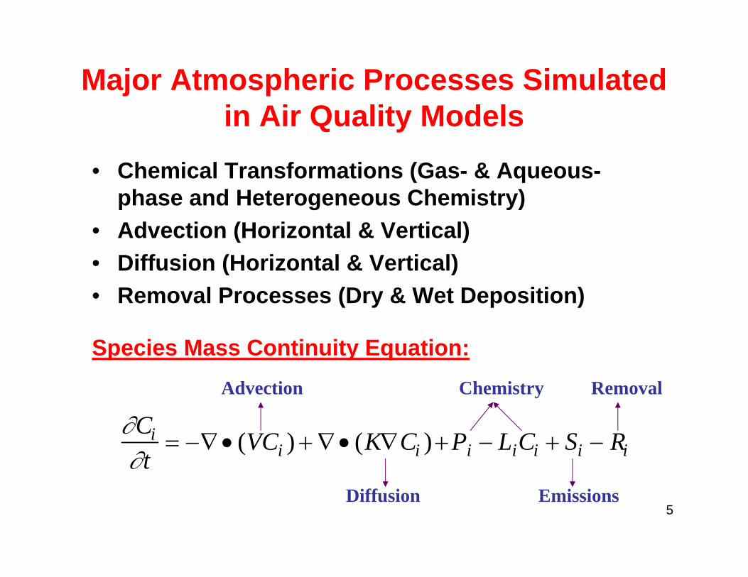
∂Ci

∂t= −∇• (VCi ) + ∇• (K∇Ci )+Pi − LiCi + Si − Ri

Advection Chemistry Removal

Diffusion Emissions

• Chemical Transformations (Gas- & Aqueous-phase and Heterogeneous Chemistry)

• Advection (Horizontal & Vertical)• Diffusion (Horizontal & Vertical)• Removal Processes (Dry & Wet Deposition)

Species Mass Continuity Equation:

Major Atmospheric Processes Simulated in Air Quality Models

6

Gaussian Dispersion ModelGaussian Dispersion Model

ISC3, CALPUFF, AERMOD CMAQ, CAMx(for primary pollutant) (multi-pollutant one-atmosphere)

FirstFirst--Generation Air Quality ModelsGeneration Air Quality Models

Photochemical Grid ModelPhotochemical Grid Model

7

PCM/Source Apportionment Advantages

• Full state of the science gas-phase chemistry– Ability to estimate realistic ozone concentrations– No need for a constant ozone background value for PM

• Advanced aqueous phase chemistry provides realistic sulfate estimates; wet and dry deposition processes included

• Photochemical models generally have good temporal and spatial estimates of ammonia concentrations

• Spatial/temporal representation of ammonia and nitric acid concentrations and state of the science inorganic chemistry (ISORROPIA) allow for realistic nitrate partitioning between gas and particle phase

• Source apportionment tools allow for tracking of single emissions sources or groups of emissions sources

8

PCM Source Apportionment Background

• Photochemical models estimate [single] source contribution with source apportionment routines

• Source apportionment tracks the formation and transport of PM2.5/ozone from emissions sources and allows the calculation of contributions at receptors

• Chemically speciated PM2.5 contribution can be converted to light extinction for visibility applications

• Precursor emissions tracked to chemically speciated PM2.5, ozone, toxics

NOX NO3-

SOX SO4=

NH3 NH4+

Primary OC POCPrimary EC PECPrimary Other POTHVOC SOA

NOX O3VOC O3

9

Particulate Source Apportionment

• Particle and Precursor Tagging Methodology (PPTM) has been implemented in CMAQ v4.6

• Particulate Source Apportionment Technology (PSAT) has been implemented in CAMx v4.5

• Tracks contribution to mercury and PM sulfate, nitrate, ammonium, secondary organic aerosol, and inert species

• Estimates contributions from emissions source groups, emissions source regions, and initial and boundary conditions to PM2.5 by adding duplicate model species for each contributing source

• These duplicate model species (tags) have the same properties and experience the same atmospheric processes as the bulk chemical species

• The tagged species are calculated using the regular model solver for processes like dry deposition and advection as bulk species

• Non-linear processes like gas and aqueous phase chemistry are solved for bulk species and then apportioned to the tagged species

10

Ozone Source Apportionment

• Ozone source apportionment has been implemented in CAMx v4.5 (OSAT & APCA) and CMAQ v4.6 (OPTM)

• Tracks ozone contribution from sources similarly to PM with reactive tracers

• July maximum ozone contribution from a source shown at right

• OSAT is simulated separately from particulate source apportionment

11

Total Light Extinction

Annual Maximum Light Extinction (1/Mm)

Ammonium Nitrate Ammonium Sulfate

Elemental CarbonPrimary Organic CarbonOther: Metals/Soil/Etc

12

Qualitative comparison to screening metric Emissions/Distance

Total Light ExtinctionEmissions/Distance

13

Issues using PCM for Single Source Apps.

• Photochemical models resource intensive (computational, disk space, staff) for multi-year applications, especially at grid resolutions <= 12km

• Additional level of staff expertise

• Existing community emissions inputs (from States, RPOs, etc) for photochemical models are actual emissions and may need to be modified if more conservative emissions estimates are necessary

• Useful for near-field applications?

14

Near Field & Long Range Transport

• Further research is necessary to determine how useful PCMs are for near-field modeling (<50 km)

• Currently, some photochemical models support full science sub-grid plume treatment, sub-cell receptor locations, and 2-way nesting capability

• Review existing near-field applications using PCMs, evaluate tracer studies

15

Other Work

• Midwest RPO did some preliminary testing (not an evaluation of CAMx PSAT or CALPUFF) of single source modeling with CAMx PSAT to compare with CALPUFF visibility estimates

• Several States did single source visibility modeling for sources less than 50 km from Class I areas; used sub-grid plume treatment

16

MRPO: CALPUFF (left) and CAMx PSAT (right)

• Annual 2002 Simulations using latest version of CALPUFF (incl. POSTUTIL and CALPOST)

• Meteorological input data is hourly and from an annual 2002 MM5 simulation

• Grid is consistent with photochemical model grid: 97 X 90 x 16 (36km grid cells) over Eastern U.S.

• Results show the number of timeseach grid cell exceeds the 24hr average .5 DV degradation over “background” visibility

• Results are the combined visibility degradation from sulfate and nitrate

• These runs were facility total actual emissions

• Applied CAMx4 PSAT sulfate for April-Sept 2002

• These results do not show the impact from nitrate; Assume that visibility degradation is dominated by summer sulfate

• Results for each facility are shown similar to CALPUFF results: counts of > .5 DV change over natural background conditions

• fRH values derived using daily average relative humidity in the grid cell as predicted by MM5 and calculated using the exact same look-up table that is used in CALPOST; the maximum daily average RH is 90

17

Total 24hr avg .5 DV ExceedancesCALPUFF (top) CAMx4 PSAT (bottom)

*CALPUFF includes sulfate+nitrate and CAMx4 includes sulfate

18*CALPUFF includes sulfate+nitrate and CAMx4 includes sulfate

Total 24hr avg .5 DV ExceedancesCALPUFF (top) CAMx4 PSAT (bottom)

19

MRPO Conclusions

• CAMx4 PSAT results do not show visibility degradation as far downwind as CALPUFF

• Need to consider nitrate PSAT runs for better comparison although visibility degradation is expected to be dominated by summer sulfate

• The tools agree qualitatively for certain facilities but not all of them

20

Final Remarks

• Photochemical grid models provide an opportunity for credible single source modeling with source apportionment methodology

• These models have the advantage of state of the science chemistry, but that comes with increased resource burden

• These models are routinely used for other regulatory purposes like O3/PM2.5/Regional Haze State Implementation Plans

21

END OF PRESENTATION

22

Post-Processing

• Estimate .5 DV changes over natural background conditions

• Methodology equivalent to CALPOST visibility post-processing

• A natural background value of 18 1/Mm is used for the Eastern U.S. (see CALPUFF manual)

• A count of > .5 DV change over natural background is kept for each grid cell and compared to Class I areas

• Bext Total = Bext Modeled + Bext Background• Delta DV = 10*ln(Bext Total/10) – 10*ln(Bext

Background/10)

23

Daily avg RH

PSAT Results:fRH calc from 24-hr RH v monthly gridded fRH values

Monthly avg fRH

Monthly avg fRH

Daily avg RH

24

Soil EC

Primary OC

Anthropogenic Biogenic

VOC

VOC, NOx

O3, OH, NO3

Secondary OC

OC

PM2.5 Chemical Composition

Sulfate

SO2

OH, H2O2, O3

VOC, NOx

O2, Fe, Mn

Oxidizing Agent

H2SO4

NOx O3 and OH

HNO3

VOC, NOx

NH3

Nitrate Others

•PM2.5 Nitrate formation depends on temperature, humidity, and the concentration of other nearby species

•PM2.5 Nitrate formation is favored by lower temperatures and higher humidity (winter and night-time)

•PM2.5 Sulfate and Organic Carbon is higher during the summer when there is higher availability of by-products of photochemical activity

25

SURFACE

TOPRegional Photochemical Models:

Tool for O3, PM2.5 (and Haze)

~ 9 miles

26

CALPUFF Sensitivity

• Sensitivity simulation for visibility calculation parameter BCKNH3

• Background ammonia concentrations (same value for entire domain for entire year)

• Important parameter in CALPUFF estimation of PM2.5 nitrate

27

CALPUFF Sensitivity:

BCKNH3 = 1.0 (basecase/default)

BCKNH3 = 0.5 and 1.5

Difference Plot SENS-BASE Difference Plot SENS-BASE