simulation of thermoacoustics with discontinuous …€¦ · simulation of thermoacoustics with...

Simulation of thermoacoustics withdiscontinuous Galerkin method

Michael Gineste

Kongens Lyngby 2006

Summary

This project concerns the simulation of thermoacoustical system. The aim is tohave a numerical method capable of doing broadband analysis of such systemthrough time-domain simulation. The numerical scheme used to the spatialdiscretization of the governing equations is the discontinuous Galerkin method.The acoustic theory is presented, and parts of this is used to include heat effectsinto the numerical scheme. The resulting method is then investigated throughsome experiments.

Resume

Dette projekt omhandler simulering af termoakustiske systemer. Malet er athave en numerisk metode i stand til at foretage bredbands analyse af sadannesystemer gennem simulering i tids-domænet. Til diskretisering af den akustiskemodel i rummet anvendes den diskontinuerte Galerkin metode. Teorien om-handlende lyd i forbindelse med varme-udveksling er præsenteret. Nogle fy-siske betragtninger bruges til at indkorporere en flukturerende varmekilde somakustiske kilde i den numeriske metode. Den resulterende metode er da un-dersøgt ved nogle eksperimenter.

Contents

Summary i

Resume iii

1 Introduction 1

2 Governing Equations 5

2.1 Introduction . . . . . . . . . . . . . . . . . . . . . . . . . . . . . . 5

2.2 The Euler Equations . . . . . . . . . . . . . . . . . . . . . . . . . 6

2.3 The Linearized Euler Equations . . . . . . . . . . . . . . . . . . . 10

2.4 Heat Release . . . . . . . . . . . . . . . . . . . . . . . . . . . . . 13

2.5 Elaboration on the different considerations . . . . . . . . . . . . . 22

2.5.1 Constant Mean Pressure . . . . . . . . . . . . . . . . . . . 22

2.5.2 Isentropicity . . . . . . . . . . . . . . . . . . . . . . . . . 25

3 Discontinuous Galerkin Method 29

vi CONTENTS

3.1 Discontinuous Galerkin Formulation . . . . . . . . . . . . . . . . 30

3.2 Numerical flux . . . . . . . . . . . . . . . . . . . . . . . . . . . . 34

3.3 Inclusion of sources . . . . . . . . . . . . . . . . . . . . . . . . . . 37

3.4 Post processing . . . . . . . . . . . . . . . . . . . . . . . . . . . . 41

4 Results 43

4.1 The Reference Solution . . . . . . . . . . . . . . . . . . . . . . . 43

4.2 Results . . . . . . . . . . . . . . . . . . . . . . . . . . . . . . . . . 44

4.3 Conclusion . . . . . . . . . . . . . . . . . . . . . . . . . . . . . . 54

CONTENTS vii

viii CONTENTS

Chapter 1

Introduction

This thesis concerns the derivation of a numerical framework, which can beused as a tool for preliminary analysis of thermoacoustic systems. As such,the numerical method has to provide the flexibility to represent a variety ofdifferent physical scenarios, and this without the need to modify the numericalscheme significantly. Such an tool can be useful to investigate the stability ofthe acoustical system under consideration, and eventually in an initial phase ofproduction.

The method is used to simulate the acoustics in the time-domain, whichallows for broadband excitation and following frequency analysis. So in theend, a larger picture of the model characteristics can be obtained.

The project crosses a variety of disciplines. On one hand it concerns the acous-tics within a combustor (a chamber in which combustion takes place), and onthe other, the use of numerical methods to solve the equation system describingthe sound field in the combustor. It was based on a wish to do a project on com-putational aeroacoustics (CAA), a field which has many interesting challenges.

New is the field of thermoacoustics, which is the theory regarding the inter-action between sound and heat. The theory is applicable to phenomena thatcan take place in many different devices, such as gas boilers or aeroengines.It considers the generation of pressure waves through fluctuating heat release,e.g when a combustion process has a fluctuating part. In this project, the sur-roundings for the sound field is a closed system, so that the chamber acts as a

2 Introduction

resonator and standing waves (modes) are possible. The heat input then actsas a source in this system, and this can eventually lead to acoustic instabilitiesunder certain circumstances, where the sound pressure levels reaches very highlevels and can cause structural damage or other unwanted effects. The Rijketube phenomenon is a good example of such an thermoacoustic instability, seee.g. [3].

The theory of acoustics can be thought separated into nonlinear and linearacoustics. In this project only linear acoustics is considered so that the soundfield is considered small amplitude perturbations on top of stationary values,which results in a linearization of the equations. In reality, when instabilitiesoccur these are damped by nonlinear effects, but these are not taken into con-siderations here.

The numerical scheme used for the simulation is the discontinuous Galerkin(abbreviated dG) method. This is a relatively new method for solving (partial)differential equations, and was chosen because of interest and because it hassome properties that makes it well-suited for aeroacoustic problems. A muchused method in CAA is a dispersion-relation preserving finite difference method(Tam & Webb), but has the drawback (in my opinion) of being a low-ordermethod. The dG method is a high-order method based on spatial discretiza-tion onto finite elements, thus it is possible to reduce the problem of inherent”numerical noise” polluting the sound field calculation. Additionally, it hasgood (low) dispersion error, so that it is well-suited for wave propagation. Sincethe goal is to use the time-domain simulation to do frequency analysis, suchproperties are welcome.

The justification of such a numerical tool contrary to the analytic treatment,hinges on the complexity of the acoustics, when the medium is moving, and theproperties of the medium changes with temperature, and a coupling betweenthe acoustic wave and the fluctuating heat release is present. All this affectsthe sound field, and closed expression is hard to obtain. Often mean flow effectsare neglected by assumption of low speed flows, but might lead to expressionsinadequate when also the heat release is included. Dowling showed in [1] howdifferent (analytic) calculation methods would give different results for resonancefrequencies, since especially the form of the sound-heat fluctuation coupling isdifficult to incorporate. In the numerical treatment of the model, this is not aproblem.

So the idea is to make a numerical ”wave tank” where the sound wavesare generated by a driver mechanism and a fluctuating heat release source isincluded. The calculations are performed in the time-domain as mentioned,thus allowing for frequency analysis over a larger spectrum, contrary to solvingthe wave equation in the frequency domain as a eigenvalue problem.A key issue, both mathematically and numerically, is how to include the heatrelease when this is considered a compact source.

3

The derived method is then used to investigate some comparison cases, basedon the modelling of the system.

The first chapter concerns the acoustic theory, in which the governing equationsare presented and the thermoacoustic theory described. This is follow by achapter on the numerical scheme, where the dG method is described and howthe inclusion of source term is done. This is to a large extent based on themodel being a hyperbolic equation system and the numerical scheme allowingdiscontinuities.At last, the results of the numerical experiments is presented and conclusionsof the project.

This text has been written with neither acousticians nor numerical analysists inmind, so it has been tried to explain things in a descriptive way. The notationsused are sought to be standard notations within their respective framework.The mathematical theory of hyperbolicity, which is closely related to the acous-tics, is not presented although this property is used and mentioned alot. Thereason being that an adequate explanation of this property would be a bit ex-aggeration, relative to the use of it. So it is assumed known.

4 Introduction

Chapter 2

Governing Equations

2.1 Introduction

Here, the acoustical framework and the resulting model is presented.It will start out with the fundamental equations concerning compressible gas dy-namics, from which are derived the governing equations for the linear acousticsframework through linearization.

The modelling of the gas dynamics will be presented in one space dimension only,since the cross-sectional dimension of the chamber is considered much smallerthan the acoustical wavelength. So the wave propagation is one dimensional,known as plane waves.

The equations describing the fluid motion are the conservation laws in differ-ential form, neglecting viscosity and heat-conduction. These three conservationlaws will simply be stated without derivation, which can be found in numeroustextbooks.

The linearized equations are known to support three kinds of waves, referred toas acoustic waves, entropy waves, and – in higher spatial dimensions – vorticitywaves. In the one dimensional case no vorticity wave exists, and will not bementioned.

6 Governing Equations

When the combustion effects comes into the acoustics, it is based on theory fromthermodynamics and this theory is to a large extent not explained. So the lawsof thermodynamics and the differently connections between thermodynamicalstate variables are used implicitly in the derivation, but not commented on.

To describe to medium in which the acoustic perturbations travel, terms like”the gas”, or ”the medium” are used interchangeably. Also the combustionprocess is called different thing; heat release, heat input or heat source are used,but all refers to the addition of energy in the form of heat.

2.2 The Euler Equations

Initially, the governing equations are presented without any source terms, whichwill be included later. This is done in order to make the resulting equations morephysically founded

The first is conservation of mass, given as

∂ρ

∂t+

∂

∂x(ρu) = 0 (2.1)

where ρ is density and u velocity. This simply states that no mass is createdwithin the medium.

The second equation is the Navier-Stokes equation for conservation of momen-tum in a compressible Newtonian fluid, neglecting viscosity and heat-conduction.

∂

∂t(ρu) +

∂

∂x(ρuu+ p) = 0 (2.2)

which is an representation of Newton’s second law applied to the fluid controlvolume in regard.

The third is the energy equation, which is an application of the first law ofthermodynamics to the medium. The time rate of change of total energy isequal to the rate of change in internal energy, caused by heat input to the gas,and the work done on the system. In this inviscid fluid, the only work done isby the pressure (and eventually body forces).

∂

∂t(ρE) +

∂

∂x(ρEu+ pu) = 0 (2.3)

where the total energy E, the sum of internal energy and kinetic energy of thegas, is given as

E = e+ 12u

2 . (2.4)

2.2 The Euler Equations 7

The internal energy is a function of temperature alone, again by the ideal gasassumption, and with assumed constant thermal properties (i.e. temperatureindependent heat capacities), gives the expression

e = cV T . (2.5)

The conservation law for total energy (2.3) can be rewritten in terms of internalenergy by use of (2.4) and the momentum equation, giving

∂

∂t(ρe) +

∂

∂x(ρue) + p

∂u

∂x= ρeheat (2.6)

The internal energy equation could be the appropriate place to include theeffects of additional heat release, ρeheat being this source. This would dependenton the physics being considered, and in the subject considered here, the heatrelease is entered differently.

The three equations – (2.1),(2.2) and (2.3) – needs a fourth relation to close thesystem which will be the thermodynamic equation of state. By the ideal gasassumption, this is given as

p = (γ − 1)ρe (2.7)

= ρRT

where γ = cP/cV is the ratio of specific heats and has the additional relationships

R = cP − cV , cV =R

γ − 1, cP =

γR

γ − 1. (2.8)

Finally, the three equations form the system of conservation laws, which ishow the Euler equations usually are presented. If this system was to containadditional terms (source terms), it would be called a system of balance laws orgeneral conservation laws instead.

∂U

∂t+∂F

∂x= 0 (2.9)

with

U =

ρρuρE

, F = F (U) =

ρuρuu+ pu (ρE + p)

(2.10)

These nonlinear partial differential allows for a variety of different phenomena,even ones which looses uniqueness and develops shocks. Therefore a solution isoften sought as a weak solution to the system.In addition, later when heat release is introduced, it enters as a Dirac’s deltafunction, which introduces an discontinuity in the solution.


Interlude on weak solutions. The theory regarding weak solutions is alarge mathematical area and quite complicated. So this short section is by faran adequate coverage of the theory, but more some principles regarding weaksolutions and introduction of some conditions used throughoutly in this project.

A solution that somehow becomes discontinuous, can not fulfill the equation(2.9). Which is why we will seek an less restrictive formulation, the weak for-mulation. This formulation allows for the real solution (or the classic solution)to (2.9), but also for discontinuous solution.

The reasoning towards it can be expressed in different ways, but in abstractterms it tries to solve for a limit function, a function in the vicinity of the ”real”function in the respective function space. A weak formulation can be defined indifferent ways, but one is to use test functions. This one relates to the numericalscheme presented later.Another is presented here, to introduce some conditions used often in dealingwith both the mathematical model and the numerical scheme.The PDE in a weak formulation is defined as

∮

C

F dt− U dx = 0 (2.11)

with C a positively oriented, piecewise-smooth, and closed curve in (x, t). If Uand F are continuous and differentiable, the Green’s formula in the plane gives

∮

C

F dt− U dx =

∫ ∫

S

(∂U

∂t+∂F

∂x

)dx dt = 0 (2.12)

so it is a solution to the original equation and vice versa.Now consider the solution being discontinuous across some line in (x, t)-

space, and denoting subscript ± as the limit state in front and after this shock.Using the contour C to evaluate the integral (2.11) around the shock, this canbe expressed as

∫ t2

t1

[F ]+− dt− [U ]+− dx =

∫ t2

t1

([F ]+− − σ [U ]+−

)dt = 0 (2.13)

with σ = dx/ dt being the shock speed. This should hold for arbitrary t1, t2,which leads to that the integrand should vanish. This is known as the Rankine-Hugoniot (abbreviated RH) conditions,

[F ]+− = σ [U ]

+− (2.14)

which has to hold across a shock, if it is to conserve mass, momentum andenergy.

The weak solution is not necessarily unique. In order to ensure a unique solu-tion, the weak formulation is usually supplemented by an appropriate entropy

2.2 The Euler Equations 9

condition. In the dG method used to find a weak solution, this is incorporatedin the method.

In addition, the system is hyperbolic, i.e. were (2.9) expressed in a quasi-linearform Ut + A(U)Ux = 0, where A(U) is the jacobian matrix. Then the latterwill have real and distinct eigenvalues. These eigenvalues reflects the speed atwhich information travels in the system. This property of hyperbolicity is quiteessential in some aspects of the numerical modelling.

These conserved quantities (mass, momentum and energy) are less ”physical”or natural in regard of what we hear and can measure, so the original conser-vation laws are formulated in a non-conservative form in terms of the primitivevariables; density ρ, velocity u and pressure p. No information is lost from theequations during this change of variables.The mass equation remains unchanged, the momentum equation in terms ofvelocity is derived from (2.2) by subtracting the continuity/mass conservationequation (2.1). At last, the equation describing the pressure evolution is de-rived from conserved internal energy equation (2.6) and the equation of state(2.7). So the system of conservation equations (2.10) in a non-conservative form,expressed in primitive quantities, is

∂ρ

∂t+ u

∂ρ

∂x+ ρ

∂u

∂x= 0 (2.15a)

∂u

∂t+ u

∂u

∂x+

1

ρ

∂p

∂x= 0 (2.15b)

∂p

∂t+ u

∂p

∂x+ γp

∂u

∂x= 0 (2.15c)

This change of variables does change the elements in the coefficient matrix ofthe system (2.15), but not its structure, since this coefficient matrix and thejacobian matrix mentioned earlier are conjugate.

The eigenvalues of this system are

λ1 = u− c , λ2 = u , λ3 = u+ c (2.16)

which reflects two sound waves travelling at their characteristic speeds λ1 andλ3 down- and upstream respectively, and one convective-acoustic wave λ2 in thesystem.


2.3 The Linearized Euler Equations

In order to simplify things and to decouple the acoustics from the aerodynam-ics, the variables describing the gas dynamics are considered separated into astationary, equilibrium field and a much smaller time-dependent, acoustic per-turbation.

pressure : p(x, t) = p(x) + p′(x, t) , density : ρ(x, t) = ρ(x) + ρ′(x, t)

velocity : u(x, t) = u(x) + u′(x, t) , temperature : T (x, t) = T (x) + T ′(x, t)

entropy : s(x, t) = s(x) + s′(x, t)

which can be justified if the perturbations are small relative to the stationaryvalues e.g. p′/p 1, which is the case as long as we’re considering soundpressure levels below human threshold ∼ 140dB. These stationary fields are thefields generally refered to when the term ’mean’ is used, e.g. mean flow velocityis u.

Inserting these separated quantities into the equations (2.15), neglecting higher-order terms, and subtracting the equations (2.15) for the mean values, results inthe so-called linearized Euler equations (LEE) for the acoustic field. Note thatthis procedure implies that the mean flow satisfies the original equations.This results in the system

ρ′

u′

p′

t

+

u ρ 00 u 1/ρ0 γp u

ρ′

u′

p′

x

+

ux ρx 0uux/ρ ux 0

0 px γux

ρ′

u′

p′

=

000

(2.17)

Hence the mean flow gradients, if present, will act as additional source terms inthe system.

When the medium is at rest (stagnant), the linearized mass and momentumequation, along with the energy equation ∂s′/∂t = 0, gives the equations thatdescribes the acoustics in the medium

[u′

p′

]

t

+

[0 1/ργp 0

] [u′

p′

]

x

=

[00

], (2.18)

which is the equation system used as limit of a vanishing flow. Mean pressureis constant in absence of flow and obviously there is no convected entropy wave.

Along these linearized equations are the linearized state equations/thermodynamic

2.3 The Linearized Euler Equations 11

relations

p′ =p

ρρ′ +

p

TT ′ = c2ρ′ +

ρc2

cPs′ (2.19)

s′ =cVp

(p′ − c2ρ′

)= cP

(T ′

T− (γ − 1)p′

γp

)(2.20)

and variations of these.

The squared sound speed is defined as ∂p/∂ρ|s, which for a perfect gas givesthe usual expression

c2 =γp

ρ(2.21)

The linearization gives, in principle, fluctuations in this sound speed, but theseare ignored, and thus c2 = c2 = γp/ρ is the definition of the sound speed usedthroughoutly.

The linearization evidently removes the nonlinearity, but also makes the fluxcoefficient matrix (locally) constant in contrast to earlier, while the mathemat-ical structure/wave nature remains the same (i.e. it is still hyperbolic), so theeigenvalues are the same, although given by the mean flow values only.

Thus the equations (2.17) (or (2.18) for stagnant medium) constitutes the gov-erning equations for the sound field in this project. This system of PDEs isconsidered over the domain (x, t) ∈ [0, L]×R+ by the plane waves assumption,along with appropriate boundary conditions. The number of conditions imposedat a boundary is determined by whether the boundary is an inlet or an outlet.In the following u(x) > 0, so nu(0) < 0 and xIN = 0 is the inlet and xOUT = Lthe outlet.Additionally, the flow is considered subsonic throughout the domain, so the localMach number M(x) = u(x)/c(x) is always <1.

The system requires boundary conditions in order to be well-posed and to des-cribe the physical surroundings. The number of required boundary conditionsare prescribed by the number of entering characteristics, with respect to theboundary normal. The mean flow enters at the left boundary, so two character-istics are incoming (λ2 = u and λ3 = u+ c), hence two boundary conditions areneeded here. While at the outlet, only one characteristic is incoming λ1 = u− c,so here only one boundary condition is required.

The simplest conditions are those describing open and closed ends of the duct.These are still idealised describtions but sufficient for the purpose.Later in this report, the condition imposed at the outlet is that of being an openend (also called pressure release), which is represented by requiring the pressure


fluctuation to vanish.p′(xOUT, t) = 0 (2.22)

Were this considered a closed end, this is equivalent to requiring the fluctuationvelocity to vanish

u′(xOUT, t) = 0 (2.23)

Such conditions give rise to reflections, the open end gives an acoustic wavereflection in antiphase of the incoming, while the closed end reflects the incom-ing wave in phase. A third possibility (in term of reflection) is obviously noreflection, which can be expressed by stating that the boundary impedance isthe characteristic impedance of the medium. Imposing boundary conditions ina numerical scheme in term of impedance conditions is a study for itself, and ifnon-reflecting boundaries were needed, the boundary formulation would dependon other aspects of the model i.e. its hyperbolicity.

Another condition used is that of the flow being choked. This can be expressedin the form of a zero fluctuating mass-flux

uρ′ + u′ρ = 0 (2.24)

This kind of boundary condition implies something about the inlet geometry.A boundary conditions of this kind is used to describe that the incoming flowpasses through a nozzle.

Another used condition at the inlet is that the inflow is isentropic. If no entropyfluctuation exists at the inlet, the sound field will be isentropic until it passessome source (explained later). So if we want the incoming sound field withrespect to the flame to be isentropic, the boundary condition has to ensureisentropicity. The approach taken here is to use the relation p′ = c2ρ′ in someway.

Nondimensional Equations

The linearized Euler equation can be put into nondimensional form, where themean flow influence is characterized by the Mach number. The following scalingsare introduced

ρ =ρ′

ρ0, u =

u′

c0, p =

p′

ρ0c20, x =

x

L, t =

t

L/c0(2.25)

where the subscript ’0’ refers to mean flow values at the inlet. Inserting anddividing through with the diagonal matrix

S = diag

(L

ρ0c0,L

c20,

L

ρ0c30

)(2.26)

2.4 Heat Release 13

results in the system of non-dimensional equations

ρup

t

+

M 1 00 M 10 1 M

ρup

x

+L

c0

ux c0ρx/ρ0 0Mux/ρ ρ0ux/c0 0

0 px/ρ0c0 γux

ρup

=

000

(2.27)where M = u(x)/c0 is the local Mach-number.Such an nondimensionalization is useful to reduce the different scalings in thesystem, and can be appropriate in many cases when a physical problem is dealtwith numerically, since it reduces the potential scale disparities. For the purposehere, where the acoustics are simulated in time to obtain time-series, this wouldbe benificial if a low-order numerical scheme was used, where the low scalesof acoustic perturbations might drown in numerical noise (round-off errors andsuch). But such an nondimensionalization also scales the frequency (by thetime scaling), and most importantly the resulting wavelength. A general rule-of-thumb in numerical analysis is that the domain discretization should allowfor at least 5 grid-points per wavelength in order to resolve a wave, and thusthe spatial discretization becomes very fine and hence computationally moreexpensive. So later when then governing equations are discretized, they willbe in dimensional form, although the scaling presented above are used in someaspects of the method.

When the heat release is introduced in the equations, an appropriate scalingcould be taken as energy density per time.

2.4 Heat Release

The acoustical theme of this project is thermoacoustics, a term implying thatwe consider the conversion of energy in form of heat into acoustic energy.In general, the medium is considered a premixed gas of reactants, which isignited at some point in the domain, so that the combustion will raise the tem-perature downstream of the combustion zone. The combustion process itselfis not taken into account. It is assumed that the unburnt and burnt gas bothbehaves as perfect gases, and that no molecular weight change occurs in the com-bustion process. If the combustion process were to be included more carefully,a model describing the chemical reaction along with evolution equations for thegas components would be needed. Here, the combustion is treated as kind ofblack-box process, the only outcome being heat addition and its consequences.

A portion of the gas in thermodynamic equilibrium will not have its temperatureaffected be the passing through of a sound wave i.e. a compression wave. Thismeans that the compression acts as an adiabatic process, so that the entropy


remains constant (no entropy fluctuation). Which is why the acoustic field gen-erally is considered isentropic.Contrary, an unsteady heat release will cause temperature fluctuations unre-lated to the pressure wave, which are convected by the flow. Therefore down-stream of the flame there will also be an entropy waves present in the system,which is the mentioned convective wave with speed u in the Euler equations innon-conservative form. These entropy fluctuations will appear in the densityfluctuation, which can have different effects.

The energy equation would be the most natural place to consider the heatrelease, since it is an energy source.However, the path towards inclusion of the heat release source term presentedbelow is the same as in [1]. This derivation is chosen, because it is based onthermodynamic considerations rather than just adding an energy source, andmore clearly presents the deviation from the usual assumption of isentropicityin acoustics.The heat input will affect the thermodynamics of the gas, so if the density isconsidered a state function of both pressure and entropy ρ = ρ(p, s), the chainrule will give

Dρ

Dt=

1

c2Dp

Dt+∂ρ

∂s

∣∣∣∣p

Ds

Dt(2.28)

since ∂ρ/∂p|s = 1/c2.Since the gas is considered inviscid and non heat-conducting, the change inentropy is given by the second law of thermodynamics

ρTDs

Dt= q(x, t) (2.29)

where q(x, t) is the heat input per unit volume.The gas is considered perfect, hence ∂ρ/∂s|p = −ρ/cp = −ρT (γ − 1)/c2, andthe expression (2.28) results in

Dρ

Dt=

1

c2

(Dp

Dt− (γ − 1)q

). (2.30)

Combined with the continuity equation (2.1), this results in a evolution operatoron the pressure similar to the previous derived expression (2.15c), but now withthe sought source term caused by the heat release

∂p

∂t+ u

∂p

∂x+ γp

∂u

∂x= (γ − 1)q . (2.31)

This heat release is considered the cause of temperature changes in the medium.So a change in the stationary temperature field is the consequence of a stationary

2.4 Heat Release 15

heat release, which changes the properties of the medium but does not act as asource of sound.

However, if the heat release has an unsteady component, this will in turn actas an acoustic source. So when the heat input enters the linearized equations,the source term will consist of the unsteady part, while the steady part is enteredimplicitly through the mean values.

When the axial extent d of the combustion zone is very small compared to theacoustic wavelength – i.e. kd 1, k being the wavenumber ω/c – it is said tobe acoustical compact. Thus this energy source can be viewed as a source ontoa plane, represented by a Dirac δ-function. Although the stationary heat releasecould be distributed, the unsteady part is only considered non-zero at the flameposition. If distributed steady heat release is part of the model, one would haveto consider the conservation laws across this distribution. But here, the generalexpression used for the heat release is

q(x, t) =(q(x) + q′(x, t)

)δ(x− β) (2.32)

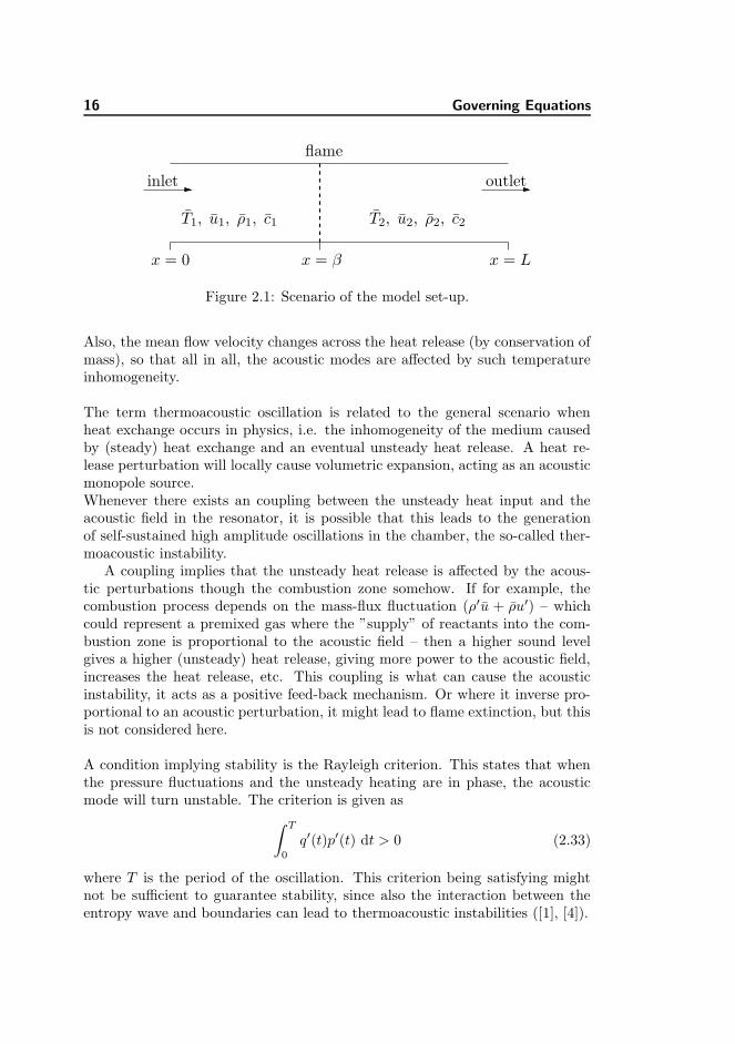
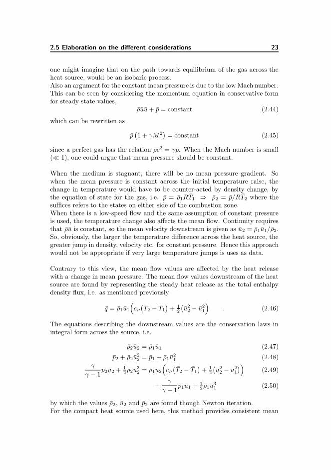
where x = β is the position of the flame. The steady heat release q hence isdiscontinuous at the flame position, reflecting a sudden temperature change. Ifisothermal walls are considered, the steady heat release represents the energynecessary to divide the domain up- and downstream of x = β, into regions withdifferent but uniform mean flow values. If losses due to cooling by the ductwalls was included, this could be modelled by a smoothly varying steady heatrelease downstream of the combustion zone. A schematic representation of themodel and the notations used is presented in Figure 2.1.

Note that the use of compactness is based on the acoustical wavelength, soin terms of the sound field it is well-founded. But the convective wave has awavelength dependent on the mean flow velocity, and for low Mach number, theassumption of compactness ωd/u 1 for the entropy wave is valid for very verylow frequencies.

When the source enters the system, mathematical and numerical, it doesso through balance of fluxes across the source, and as such on assumption ofcompactness. The entropy wave can have a strong influence on the acousticsunder certain circumstances, and as such this lack of compactness is a factorthat should be considered, since it might affect the numerical simulations.

The steady heat release changes the temperature, which in turn changes theproperties of the gas regarding sound propagation. The characteristic impedanceof the medium has a jump at the flame position, which causes an incomingsound wave to be partially transmitted and reflected. Considering the mass andmomentum equation in a small volume around the impedance jump, it can beseen that the jump in pressure and velocity perturbations vanishes, as one couldexpect.


x = 0 x = β x = L

inlet outlet

flame

T1, u1, ρ1, c1 T2, u2, ρ2, c2

Figure 2.1: Scenario of the model set-up.

Also, the mean flow velocity changes across the heat release (by conservation ofmass), so that all in all, the acoustic modes are affected by such temperatureinhomogeneity.

The term thermoacoustic oscillation is related to the general scenario whenheat exchange occurs in physics, i.e. the inhomogeneity of the medium causedby (steady) heat exchange and an eventual unsteady heat release. A heat re-lease perturbation will locally cause volumetric expansion, acting as an acousticmonopole source.Whenever there exists an coupling between the unsteady heat input and theacoustic field in the resonator, it is possible that this leads to the generationof self-sustained high amplitude oscillations in the chamber, the so-called ther-moacoustic instability.

A coupling implies that the unsteady heat release is affected by the acous-tic perturbations though the combustion zone somehow. If for example, thecombustion process depends on the mass-flux fluctuation (ρ′u + ρu′) – whichcould represent a premixed gas where the ”supply” of reactants into the com-bustion zone is proportional to the acoustic field – then a higher sound levelgives a higher (unsteady) heat release, giving more power to the acoustic field,increases the heat release, etc. This coupling is what can cause the acousticinstability, it acts as a positive feed-back mechanism. Or where it inverse pro-portional to an acoustic perturbation, it might lead to flame extinction, but thisis not considered here.

A condition implying stability is the Rayleigh criterion. This states that whenthe pressure fluctuations and the unsteady heating are in phase, the acousticmode will turn unstable. The criterion is given as

∫ T

0

q′(t)p′(t) dt > 0 (2.33)

where T is the period of the oscillation. This criterion being satisfying mightnot be sufficient to guarantee stability, since also the interaction between theentropy wave and boundaries can lead to thermoacoustic instabilities ([1], [4]).

2.4 Heat Release 17

Modelling the combustion reaction can be a tricky affair, and many differ-ent suggestion can be found in the literature. This often involves combustionchemistry, with the medium composition and more complex combustion reac-tion expressions. In this project, the unsteady heat release model serves thepurpose of creating the coupling and thus amplifying the resonant modes in thechamber, i.e. as the phase-locking mechanism so that the fundamental modesare the most dominant. The flame model primarily used here is that of thereference solution, since it is against this that the varying factors are comparedand the method evaluated.

Balance conditions

Consider the source term the equation (2.31) and let this be represented by adelta function q(x) = q(x)(x − β), so that the solution is discontinuous acrossthe source position. Hence the equation are not valid across the source, since thesolution is not continuous nor differentiable across the source. But this is not ofgreat concern, since a weak solution is sought. So instead, the physical principlesare supposed to hold, by requiring the flux of basic conservation quantities,expressed in integral formulation (or equivalently, a weak formulation), to beconserved or balanced in the limit over the source position. These are theRankine-Hugoniot conditions across this imposed, stationary shock. For theheat release, this reads

[ρu]β+

β− = 0 (2.34a)

[ρuu+ p]β+

β− = 0 (2.34b)

[u(ρE + p

)]β+

β−= q (2.34c)

where the factor (γ−1) has been dropped with respect to (2.31). When dealingwith gas dynamics, these conditions tells something about the state on eitherside of a shock and here they express the differences in fluxes caused by a sourceterm.

The energy balance (2.34c) tells us something about the scale of the heat release.The model has the temperature as a tunable parameter, so it would be naturalto look at the total enthalpy density flux ρu(e+ p/ρ+u2/2). For a perfect gas,this gives

u(ρE + p

)= ρu

(cPT + 1

2u2)

(2.35)

so it is a bit intuitive to take q ∝ ρ1u1

(cP(T2 − T1

)+ 1

2

(u2

2 − u21

))considering

in/out of the combustion zone.


The governing equations for the acoustics are linearized, so the Rankine-Hugoniotconditions above is not used as presented, but in a linearized form. The steady-unsteady splitting is introduced in these expressions (2.34), and the steady stateform of the conditions is subtracted, again by the steady field implicitly havingconservation of mass and momentum, and balanced energy, for the heat release.These RH-conditions for acoustic perturbations are presented here, and theiruse is described in later section on the numerical scheme.

[ρ′u+ ρu′]β+

β− = 0 (2.36a)

[p′ + ρ′u2 + 2ρuu′

]β+

β−= 0 (2.36b)

[(cP T + 1

2 u2)(ρ′u+ ρu′

)+ ρu

(cPT

′ + uu′)]β+

β−= q′ (2.36c)

The energy flux can also be describes in term of the used dependent variables.Either by the reformulation u

(ρE + p

)=(

γγ−1pu + 1

2ρu3)

and linearizing, or

equivalently by use of (2.36c) and the relation cPT′ = p′/ρ + T s′ and cP T =

γp/ρ(γ − 1). This results in the equation

[γ

γ − 1

(up′ + pu′

)+ u2

(12 uρ

′ + 32 ρu

′)]x+

x−= q′ (2.37)

which also is the used form in the implementation. The case of a stagnantmedium (i.e. no flow) is also considered. The RH-conditions on the conservedquantities are not directly applicable in this case. The jump conditions, whenthe medium is at rest reduces significantly (see [1] for derivation), such that forunsteady heat release, the conditions becomes

[p′]x+

x− = 0 and [u′]x+

x− =(γ − 1)

ρ1c21q′ . (2.38)

These jump conditions hence describes the coupling between the variables acrossa source, which is how they are used when a numerical model of the problem isconstructed. As mentioned, the unsteady heat release is a sound source throughvolumetric expansion, and as such, the jump in primitive variables are expectedto be largest (relatively) in the density fluctuations.When a mean flow is present, the density fluctuation downstream of the pointof application of these conditions will carry an ”excess density” (deviation fromρ′ − p′/c2), which is the entropy wave.

Driving sources

As mentioned, the unsteady heat release acts as an acoustic source, but only inpresence of an acoustic field by the coupling of these. So there is need for an

2.4 Heat Release 19

extra source in order to generate the sound field.

Maybe the most simple way to generate an acoustic perturbation in the chamberis to let an inflow boundary condition (at x = xIN) act as an abstraction of apiston, still allowing a mean flow to pass through i.e. an inlet boundary conditionon the form u(xIN, t) = u(xIN) + u0e

−iωt with ω being the frequency and u0 theamplitude of this acoustic perturbation.

In this project, again, the specific type of boundary condition is importantfor the resonator and it seemed reasonable not to start mixing a driver signal andthe more physical boundary conditions. It might even deteriote the simulation,since incoming waves would ”feel” the piston as well.

A modification of this approach, still in order to generate an acoustic field, is touse the hyperbolicity of the system, decomposing the system into its character-istics, and then imposing the driving source as the incoming wave and lettingthe outgoing passing through. If the model had non-reflecting boundaries as arequirement, this method would be more appropriate.

The inclusion of driving sources is done by adding source terms to either the massor momentum conservation equation, which corresponds1 to either externallymass-injection or force representation ([3, p. 28]). So for an external mass-injection, the inhomogeneous conservation law becomes

∂ρ

∂t+

∂

∂x(ρu) =

∂ρfρ∂t

(2.39)

where the right hand side is the rate of injected mass by volume fraction fρ.And for an external force source per unit volume

∂

∂t(ρu) +

∂

∂x(ρuu+ p) = fu (2.40)

These two sources are fixed in space and considered compact (δ-sources), andare used to drive the system with a broadband signal. The exact expression ofthis signal is given later.During the linearization process, the momentum source does not change (andhence is considered small-scale), while the mass-injection term results in ρ dfρ/dt,again with fρ being small.

The inclusion of a mass term in (2.39) affects the formulation of the momen-tum conservation in non-conservative form (2.15b) by adding a term−u∂ (ρfρ) /∂tor in linearized form −uρ∂fρ/∂t. However, when the source is included in thenumerical scheme, it enters through considerations about the conservative formof the system. So the term does not matter as such, and is ignored here.

1these are simplifications, the actual physical process can be rather complicated


Either one of these source terms can be applied through the appropriate jumpconditions (2.36a) or (2.36b), and be included into the numerical method in thesame way as the unsteady heat release, as will be explained later.

By considering the conservation laws (2.39) and (2.40) in a integral formula-tion, one can arrive at more simple jump conditions/estimates for such externalsources [3, p.84]. For the mass injection at instant time this reads

[u′]+− = fρ and [ρ′]

+− = [p′]

+− = 0 (2.41)

with the superscripts ± denoting either side of the source position. Very similar,the jumps describing an external force are

[p′]+− = fu and [u′]

+− = [ρ′]

+− = 0 . (2.42)

The jump expression (2.41) is used in stagnant medium to represent a mountedloud-speaker with some volume velocity fρ, and when an isentropic model withmean flow is considered (presented in later section), these are the conditionsused to enter the driver in the numerical scheme.The signal used to drive the chamber is considered in greater detail in thefollowing section

The placement of the acoustic drivers for the stagnant medium is not impor-tant, this just creates an acoustic disturbance. But when there is a flow, theplacement matters. The driver is imposed via jump conditions, so the solutionis discontinuous across the driver. This discontinuity creates entropy fluctua-tions since entropy cannot be conserved across a shock. This entropy fluctuationconvects with the flow, so this has to taken into account if the model expectsthat the acoustic wave entering the combustion zone is isentropic. Placing thedriver downstream of the heat release source removes this particular problemwith respect to the heat source.

Some of the forms for including a driver source generates stronger entropy wavesthan others. The simple velocity jump condition (2.41) generates only weakerentropy waves. Hence, if outlet boundary conditions would have an effect bythe impinging entropy wave, it would be more appropriate to use the simpler(2.41) in order not to add to this boundary effect unnecessarily..

Driving signal

The reason for solving this acoustic problem in the time-domain, relies on itsnon-restriction (in regard of formulation) to single frequency perturbations. Sothe idea is to excite the chamber with a signal which covers some frequency band,

2.4 Heat Release 21

so that the unknown, and possibly more, resonance frequencies are excited. Alinear broadband signal is chosen here. In principle, a block signal (or binarysignal) would have a broader spectrum, but the propagation of such a signalis more complex in regard of the numerical treatment. Besides, it is expectedthat the different conditions under consideration, will shift the fundamental,geometric eigenfrequency, but not with large jumps. So the excitation spectrumcan be set thereafter, and a signal with a relatively narrow spectrum would stillexcite the sought instability frequencies, and give, in the end of the process,spectras just as good. So occam’s razor applies, and the simpler, linear drivingsignal is used.The expression for the driver signal, also known as a sweep signal, is given as

y(t) = A sin((∆ω t+ ωmin) t

)(2.43)

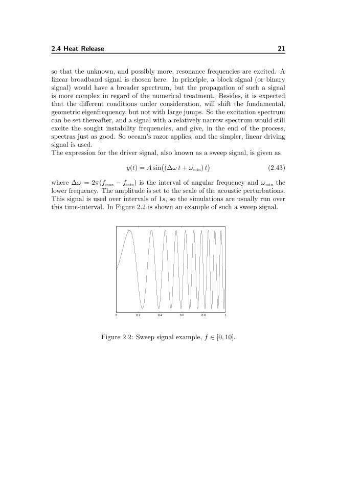
where ∆ω = 2π(fmax − fmin) is the interval of angular frequency and ωmin thelower frequency. The amplitude is set to the scale of the acoustic perturbations.This signal is used over intervals of 1s, so the simulations are usually run overthis time-interval. In Figure 2.2 is shown an example of such a sweep signal.

0 0.2 0.4 0.6 0.8 1

Figure 2.2: Sweep signal example, f ∈ [0, 10].


2.5 Elaboration on the different considerations

The reason for the definition of the numerical experiments is twofold. Oneis to set up some different considerations that could have an acoustical effectand use the numerical simulations to investigate this. And secondly, to havesome different perspective regarding the numerical method itself. The subjectof comparison are thus chosen as to describe not too different model set up inregard of physics, in order to see how this influences both the sound field itselfand the simulation of it.

In terms of the acoustics, the question is, does some assumptions or aspects inregard of the model affect the system in terms of possible resonant modes, andif this is the case, how much. Or can a simpler model be used without losing theeffects of whatever phenomenon is taking place or can an deviation be predictedand ”corrected” for.

Here, the two assumption in question, are the constant mean pressure assump-tion although a temperature change being present, and the very general assump-tion of an isentropic medium.

The combustion that takes place might raise the gas temperature signifi-cantly, and that this change in temperature should solely be balanced by den-sity change even in the low Mach limit, is less likely. This is a question that isrelated to the (given) stationary flow values in the model and especially relatedto modelling the stationary heat release.

The assumption of isentropicity is related to the fluctuating quantities. Theunsteady heat release can cause convected temperature perturbations not as-sociated with the pressure fluctuations (the entropy waves) which can have aneffect on the resulting sound field. This is thought to have an effect for lowfrequencies only.So this ”versus”-case is meant to indicate whether the full system of equationsshould be used or if a reduced (appropriate) model is satisfactory.

2.5.1 Constant Mean Pressure

Although the differential equations are invalid across the flame position, theconservation laws still tells something about the inter-dependency of the steadystate values. And if the mean velocity change, so should the mean pressure.

A constant mean pressure is sometimes assumed for small temperature gradientin a relatively narrow geometry. Here the temperature changes abruptly, and

2.5 Elaboration on the different considerations 23

one might imagine that on the path towards equilibrium of the gas across theheat source, would be an isobaric process.Also an argument for the constant mean pressure is due to the low Mach number.This can be seen by considering the momentum equation in conservative formfor steady state values,

ρuu+ p = constant (2.44)

which can be rewritten as

p(1 + γM2

)= constant (2.45)

since a perfect gas has the relation ρc2 = γp. When the Mach number is small( 1), one could argue that mean pressure should be constant.

When the medium is stagnant, there will be no mean pressure gradient. Sowhen the mean pressure is constant across the initial temperature raise, thechange in temperature would have to be counter-acted by density change, bythe equation of state for the gas, i.e. p = ρ1RT1 ⇒ ρ2 = p/RT2 where thesuffices refers to the states on either side of the combustion zone.When there is a low-speed flow and the same assumption of constant pressureis used, the temperature change also affects the mean flow. Continuity requiresthat ρu is constant, so the mean velocity downstream is given as u2 = ρ1u1/ρ2.So, obviously, the larger the temperature difference across the heat source, thegreater jump in density, velocity etc. for constant pressure. Hence this approachwould not be appropriate if very large temperature jumps is uses as data.

Contrary to this view, the mean flow values are affected by the heat releasewith a change in mean pressure. The mean flow values downstream of the heatsource are found by representing the steady heat release as the total enthalpydensity flux, i.e. as mentioned previously

q = ρ1u1

(cP(T2 − T1

)+ 1

2

(u2

2 − u21

). (2.46)

The equations describing the downstream values are the conservation laws inintegral form across the source, i.e.

ρ2u2 = ρ1u1 (2.47)

p2 + ρ2u22 = p1 + ρ1u

21 (2.48)

γ

γ − 1p2u2 + 1

2 ρ2u32 = ρ1u2

(cP(T2 − T1

)+ 1

2

(u2

2 − u21

))(2.49)

+γ

γ − 1p1u1 + 1

2 ρ1u31 (2.50)

by which the values ρ2, u2 and p2 are found though Newton iteration.For the compact heat source used here, this method provides consistent mean


flow values, although one could question the use of an enthalpy jump for theheat release for larger temperature change, since the change in pressure becomessignificant

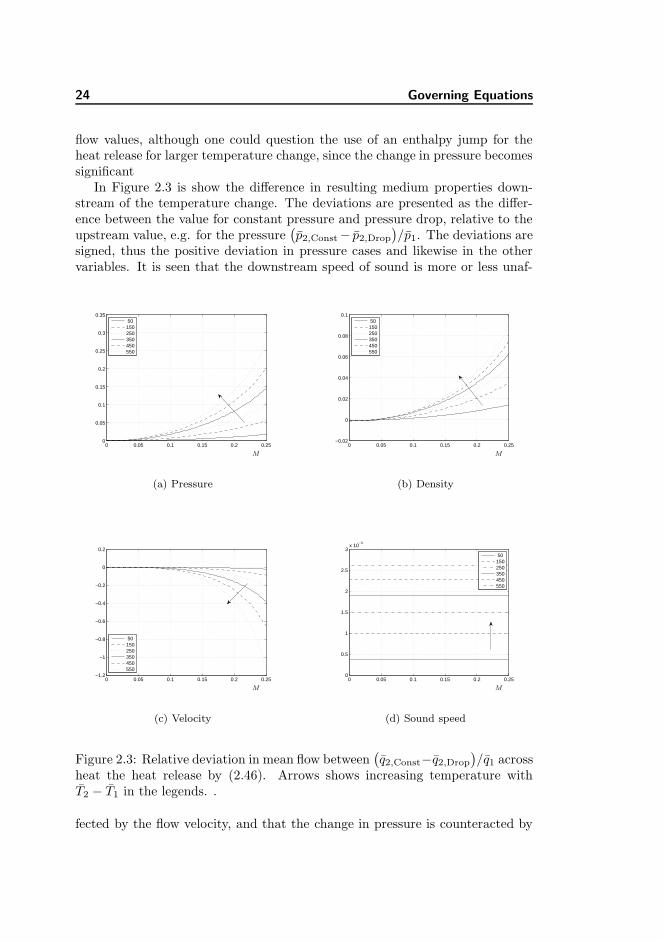
In Figure 2.3 is show the difference in resulting medium properties down-stream of the temperature change. The deviations are presented as the differ-ence between the value for constant pressure and pressure drop, relative to theupstream value, e.g. for the pressure

(p2,Const− p2,Drop

)/p1. The deviations are

signed, thus the positive deviation in pressure cases and likewise in the othervariables. It is seen that the downstream speed of sound is more or less unaf-

0 0.05 0.1 0.15 0.2 0.250

0.05

0.1

0.15

0.2

0.25

0.3

0.35

50150250350450550

M

(a) Pressure

0 0.05 0.1 0.15 0.2 0.25−0.02

0

0.02

0.04

0.06

0.08

0.1

50150250350450550

M

(b) Density

0 0.05 0.1 0.15 0.2 0.25−1.2

−1

−0.8

−0.6

−0.4

−0.2

0

0.2

50150250350450550

M

(c) Velocity

0 0.05 0.1 0.15 0.2 0.250

0.5

1

1.5

2

2.5

3x 10

−3

50150250350450550

M

(d) Sound speed

Figure 2.3: Relative deviation in mean flow between(q2,Const−q2,Drop

)/q1 across

heat the heat release by (2.46). Arrows shows increasing temperature withT2 − T1 in the legends. .

fected by the flow velocity, and that the change in pressure is counteracted by


density change, with respect to the resulting sound speed. And that the meanvelocity is significantly higher for the pressure drop case, at large temperaturejumps and higher inlet velocity.

Based on this, and since the comparison is meant for low-speed mean flow, theupper mean velocity limit is taken so that 0 ≤ M1 ≤ 0.15, otherwise the meanvelocity downstream differs to considerably for the used temperature changes.

2.5.2 Isentropicity

What if we can formulate the problem, such that no entropy wave can be present,but still considers the acoustic source effect of the heat release.

Over the flame, isentropicity can not be assumed, but it does not matter, sincehere other equations (the Rankine-Hugoniot conditions) describes the behaviorof the gas. So the above system in a linearized form is used on either side of theheat release, such that no entropy wave should be present downstream of theheat source, but the unsteady heat still acting as a source of sound

The entropy wave/mode is carried by the density fluctuation, and can generateacoustic perturbations by a coupling between boundaries and the presence ofthese temperature fluctuations. For instance a choked outlet can give pressurereflections. Here the outlet is an open end, which just convects the entropy wave.So it is the effect of its presence (or ”allowed” presence) that is questioned fora certain case of physical setup.

The isentropicity starts with ds = 0, or in term of total derivative

Ds

Dt= 0 (2.51)

This is a general form of the energy conservation equation when a non-heatconducting and inviscid medium is considered. In view of (2.28), this gives theoften used equation of state for isentropic flow

Dp

Dt= c2

Dρ

Dt(2.52)

in deriving the equations of linear acoustics. If (2.51) has to hold with noentropy fluctuations, the flow has to be homentropic as well i.e. s is constant.So the temperature is considered uniform on either side of the heat release.

The isentropic version of the Euler equations in nonconservative form can bereduced to the momentum equation and – using the energy equation as (2.52)and the mass conservation equation (2.1) to eliminate for ρ – an equation for


the pressure evolution. These are of course the same used previously, repeatedhere for convenience.

∂u

∂t+ u

∂u

∂x+

1

ρ

∂p

∂x= 0 (2.15b)

∂p

∂t+ u

∂p

∂x+ γp

∂u

∂x= 0 (2.15c)

These two equations are usually used to linearize and form the acoustic waveequation. Under the simplifying assumptions of no mean flow gradient and ho-mogeneous medium, the acoustics are described by the modified wave equation

∂2p′

∂t2+(u2 − c2

)∂2p′

∂x2+ 2u

∂2p′

∂t∂x= 0 (2.53)

Through reducing the system order by explicitly expressing isentropicity, we seethat the solution, in term of invariants/characteristic waves/ travelling waves,now only consist of two waves, travelling at speed u± c.

Previously, when the entropy wave was considered present in the solution,this could not be seen directly from the governing equations, since neither tem-perature fluctuations nor entropy fluctuations occurred in the equations as such.Nevertheless, the entropy wave was considered there and carried in the densityfluctuation through convection. It was the characteristic travelling at mean flowspeed.The unsteady temperature caused by unsteady heat release, enters through theRankine-Hugoniot conditions for the acoustic perturbations, and it is throughthe coupling here, that the entropy wave starts and is convected. Even if isen-tropicity is assumed everywhere, it can not be assumed across the heat source,and if the equations allow for the wave to exists, it will ”propagate” by convec-tion.

Now, we consider equations which do not allow for entropy waves as such, thesystem being reduced. But the RH conditions were imposed in order to respectthe conservation laws, and as such should still apply when the heat source isthere. The source is still sought included in the same way as described previ-ously, so there is one equation to many, since when included in the numericalscheme, the number of equations needed is the number of dependent variables.

This is overcome by using the RH conditions for the acoustic fluctuation(2.36), by eliminating for the downstream density fluctuation and using thefluctuating mass flux condition. This provides the two equations


p′2 + ρ2u2u′2 − p′1 − ρ′1u1(u1 − u2)− ρ1(2u1 − u2)u′1 = 0 (2.54a)

γ

γ − 1

(u2p′2 + p2u

′2

)− γ

γ − 1

(u1p′1 + p1u

′1

)+ ρ1u1u2u

′2

− ρ1u21u′1 − (ρ′1u1 + ρ1u

′1)

1

2

(u2

1 − u22

)= (γ − 1)q′ (2.54b)

The density fluctuation immediately upstream of the source is present in theequations, but the sound field here is assumed isentropic with isentropic bound-ary conditions, so it is tempting to take ρ′1 = p′1/c

21, so these equations solely

are described by p′ and u′.

This case is meant to investigate if the reduced system along with the aboveconditions gives the same acoustic behavior when simulated. Naturally, this onlyapplies for some specific cases of model. It would, for example, be rather difficultto express non-isentropic boundary conditions with such a reduced system.

Chapter 3

Discontinuous GalerkinMethod

In this chapter is presented used numerical method, the discontinuous Galerkinmethod.The discontinuous Galerkin method can be seen as a hybrid method between thefinite element and the finite volume method. It shares the geometric flexibilityof both the FEM and FVM in regard to unstructured meshes, and has theconservation properties of the FVM and the higher-order property of FEM. Ithas been applied to a large variety of problems now, and is generally consideredto be quite flexible.

The Matlab codes used in this project are based on codes presented in [2], andhow all the necessary parts of the scheme are set up, will not be a subject in thefollowing. The principles of the method will be presented, with emphasis on theproperties this particular scheme holds, and are ”appropriate” for the model inregard.

The equations will be semi-discretized i.e. the spatial operators are to be ap-proximated with the dG method, while the temporal integration is handled withsome Runge-Kutta method.

In this chapter, the first couple of sections concern a very general description ofthe dG method. Then follows the details which are relevant to the problems in

30 Discontinuous Galerkin Method

this thesis. At last is the part regarding inclusion of sources.

Regarding notation, the style will be adapted from [2], since this book has servedas textbook on the subject.

The model concerns 1D in space, so the presentation of the numerical schemeis restricted to the 1D case. By this in mind, the scheme is fully extendable tohigher dimensions.

3.1 Discontinuous Galerkin Formulation

Consider the system (2.17), expressed as

∂u

∂t+∂Au

∂x+Bu = 0 (3.1)

where u = (ρ′, u′, p′)T being the primitive variables. This is a system of coupledadvection equations with constant matrices A and B, given as

A =

u ρ 00 u 1/ρ0 γp u

, B =

0 0 0uux/ρ 2ux −ρx/ρ2

0 (1 + γ)px (1 + γ)ux

(3.2)

where the matrix B ≡ 0, if the mean flow is uniform on either side of the heatsource. In the following presentation, such a uniform flow is assumed, becauseit corresponds to the main situation in the acoustic model, and because it doesnot have change the derivation of the numerical scheme. Hence, the equation(3.1) is presented in a general conservation form

∂u

∂t+∂f(u)

∂x= 0 (3.3)

with f(u) = Au

In the following presentation of the scheme, the equation to be discretized is ascalar equation. This is only to make the notation easier, it is directly applicableon each equation in the system (3.3).

So the problem equation is

∂u

∂t+∂f(u)

∂x= 0 (3.4)

along with some initial condition u(x, 0) = u0(x) and boundary conditions.

3.1 Discontinuous Galerkin Formulation 31

The solution is sought in the spatial domain Ω : x ∈ [0, L], initially by a fi-nite element formulation. The finite element formulation consists of dividingthe spatial domain in non-overlapping and not necessarily uniform elementsDk =

[xk−, x

k+

], such that Ω =

⋃Kk=1 D

k, and expressing the solution u on eachelement as a local polynomial approximation ukh. The N ’th order polynomialrepresentation can be either on a modal or a nodal basis, such that the localelement-wise solution for x ∈ Dk is represented as

ukh(x, t) =

N∑

n=0

ukn(t)ψn(x) =

N∑

i=0

ukh(xki , t)li(x) (3.5)

where the ukn are the modal expansion coefficients, while the ukh(xki , t) are thenodal values. The basis considered here, of which different choices could bemade, are the Legendre polynomials ψn and the Lagrange interpolating poly-nomials li(x). The order of the approximation is one of the parameters tocontrol the discretization error, the other being the number of elements cover-ing the domain. This polynomial approximation is what gives the scheme thenice property of having spectral convergence, i.e. for polynomial projectionsand smooth solutions u ∈ Hp with p large – which denotes solutions with p− 1continuous derivatives and bounded p’th derivative – the approximation error‖u− uh‖ is O(N−p), which is a very fast convergence.

The solution to the equation is then the sum of these local solutions

u(x, t) ≈ uh(x, t) =

K∑

k=1

ukh(x, t) . (3.6)

The ”approximation error” by this polynomial representation is the quantity,that is wanted minimized, or more precisely, wanted to be a zero-function, inthe weak sense of a L2-norm (the inner product). This is done by expressinga residual R(uh) by the polynomial approximation inserted into the equation,then multiplying with a test function φ, locally defined on each element andcontinuous on this, and then taking the inner product. In the Galerkin frame-work, these test functions are chosen from the same function space as the oneused to express the polynomial approximation (the trial functions).So on each element, the problem is defined as

∀k, l∫

DkR(ukh)φl(x) dx =

∫

Dk

(∂ukh∂t

+∂fh(ukh)

∂x

)φl(x) dx = 0 (3.7)

where

ukh =

N∑

n=0

ukn(t)φn(x) (3.8)


is a general representation used henceforth, where the test function φ could beeither the Legendre basis functions ψ or the Lagrange basis l, as given in (3.5).

Performing integration by parts on the spatial derivative once, gives the weakform of the scheme

∀k, l∫

Dk

(∂ukh∂t

φl − f(ukh)dφldx

)dx = − [f∗φl]

xk+xk−

(3.9)

The flux evaluation at the element edge f(ukh)∣∣∂Dk

is the place where the dG-method separates itself from the finite element formulation. In the finite elementformulation, the basis usually vanishes at element edges, such that the right handside in (3.9) is zero.

Since the trial space, onto which the numerical solution is decomposed, hasno requirement of continuity across elements, this flux can be multiply definedas both f(uh(xk+, t)) and f(uh(xk+1

− , t)), since xk+ = xk+1− . This ambiguity is the

reason for introducing the so-called numerical flux or trace f ∗ in (3.9), whichis a key concept in the dG-method. How this is defined and what function itserves, will be adressed later. But from the above expression it is apparent, thatsomething having to do with an element edge, comes into the scheme by thisnumerical flux.

This deficiency of continuity requirement in-between elements is also a reasonwhy the dG method has efficiency advantages. The elements decouple in a sense,so that for large problems (in terms of grid), each element can be solved for, onits own i.e. the scheme is parallizable, a valuable property when dealing withlarge time-dependent problems.

The dG scheme has a second form, called the strong form, which results fromthe weak form (3.9) by re-doing integration by parts

∀k, l∫

Dk

(∂ukh∂t

+∂f(ukh)

∂x

)φl dx =

[(f(ukh)− f∗

)φl]xk+xk−

(3.10)

These two forms are mathematically the same, although the strong form shouldhave a tendency of better convergence. Also it is the form used in the imple-mentation, although no difference was found between using the weak and thestrong form.

Inserting the polynomial representation (3.8), and of course a similar representa-tion of the flux function, into the weak form (3.9), and interchanging summationand integration yields for each element

N∑

n=0

∂ukn∂t

∫

Dkφnφk dx−

N∑

n=0

fkn

∫

Dkφndφkdx

dx = − [f∗φl]xk+xk−

(3.11)

3.1 Discontinuous Galerkin Formulation 33

or equivalently expressed in matrix-vector notation, with ukh =(uk0 , . . . , u

kN

)T

being the vector of solution coefficients, and the same for fk

h:

Mk dukh

dt−(Sk)Tfk

h = − [f∗φl]xk+xk−

(3.12)

where the matrices are being defined as

Mkij =

∫

Dkφiφj dx , Skij =

∫

Dkφidφjdx

dx (3.13)

The strong form results in a similar form, as

Mk dukh

dt+ Skf

k

h =[(f(ukh)− f∗

)φl]xk+xk−

(3.14)

The matrices Mk and Sk are local operators, since they depends on the basisdefined on each element and in principle should be defined for each element.Without going into details with the implementation, this is overcome by definingthe basis on a reference element, such that these matrix operators operate onthe reference element and then mapped onto the physical, spatial element. Thisis however more of an efficiency concern.The independency of each element equation system – (3.9) or (3.10) – withrespect to each other, adds the property of being hp-adaptive to the scheme.This means that adjacent local solutions can be approximated in different orderand/or over elements of different lengths. So the grid spacing and approximationorder can be adjusted to parts of the problem, if needed. This can also be doneduring the calculations, with an extra computational effort of course, so thatparts of the solution can be discretized ”at a smaller scale” or eventually tracked.

This above form are reduced even further, again without considering the detailsabout construction etc. such that e.g. for the strong form

dukhdt

+ Dkfk

h =(Mk)−1 [(

f(ukh)− f∗)φl]xk+xk−

(3.15)

where the matrix Dk acts as a differentiation matrix (or a interpolation form ofthe derivative), in much the same way as in spectral methods.

This is the sought semi-discretization of the PDE, now we can apply anintegrator for the time-derivative, where the right hand side of this ”ODE” isthe spatial discretization, i.e.

dukhdt

= F (ukh, t) (3.16)

F (ukh, t) = −Dkfk

h +(Mk)−1 [(

f(ukh)− f∗)φl]xk+xk−

(3.17)


The integrator used is the 4’th order, 5 stage Low Storage Runge-Kutta methodpresented in [2]. Alternatives have been tried in form of a 4’th order, 6 stageLow Dispersion Low Dissipation Runge-Kutta (also in low storage form), butwithout distinct differences. So the cheaper 5 stage scheme was used.

The discretization in space sets a bound on the time-step, in a CFL-sense.The time-stepping should ensure that the domain of dependence (regarding thehyperbolicity of the problem) is respected. So a bound on time-step involvesthe minimum spatial discretization length, but it also has to take into accountthe speed of the propagating waves in the system. A bound can be formulatedas ([2, p.62]),

∆t ≤ Cmin ∆x

ρ(A)(3.18)

with ρ(A) being the (global) spectral radius of the flux coefficient matrix in(3.1). When frequency analysis is performed on recorded time-series, the time-step (or sampling rate) is small enough to guarantee that waves in the frequencyrange considered are represented.

3.2 Numerical flux

xk−xk−1+ xk+

x

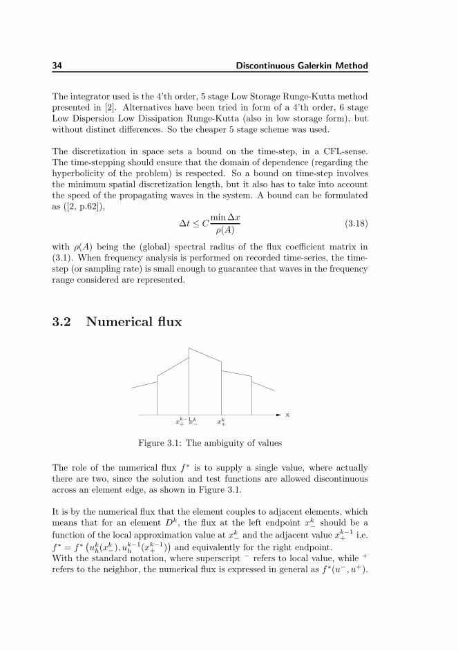
Figure 3.1: The ambiguity of values

The role of the numerical flux f∗ is to supply a single value, where actuallythere are two, since the solution and test functions are allowed discontinuousacross an element edge, as shown in Figure 3.1.

It is by the numerical flux that the element couples to adjacent elements, whichmeans that for an element Dk, the flux at the left endpoint xk− should be a

function of the local approximation value at xk− and the adjacent value xk−1+ i.e.

f∗ = f∗(ukh(xk−), uk−1

h (xk−1+ )

)and equivalently for the right endpoint.

With the standard notation, where superscript − refers to local value, while +

refers to the neighbor, the numerical flux is expressed in general as f ∗(u−, u+).

3.2 Numerical flux 35

This also means, that for boundary elements i.e. elements with edges coincidingwith ∂Ω, the boundary condition enters the scheme through the flux, wherethe condition is imposed weakly by setting the external value to an appropriatevalue e.g. for the left endpoint of the domain f ∗ = f∗

(u1h(x1−), uh,BC)

). To

impose boundary conditions in this way seems a good way to treat ”the imposingboundaries problem”, since it is done the exact same way in the interior domain.No special treatment of the boundary conditions is required as such, which canbe quite a challenge in some numerical schemes.

A proper choice of numerical flux is what ensures stability of the scheme. Sta-bility of the scheme is analyzed by use of the energy method, a method thataims at proving a stability condition in the form ‖uh(t)‖Ω ≤ c(t∗) , t ∈ [0, t∗].The details of this analysis can be found in [2, chap. 4], which also includeconsistency and convergence analysis. In brief, if the scheme is consistent andstable, convergence follows by the Lax equivalence theorem.

The choice of numerical flux, assuming that it renders the dG method stable,is somewhat arbitrary. The theory regarding the use of such fluxes stems fromthe finite volume method, since it is a crucial part of this numerical scheme.In the finite volume method, cells (or control volumes) are considered, and thesolution averaged over these cells1. At the interface between two such cells, aflux evaluation is needed.

When a homogeneous conservation law is considered, this can be expressedas a Riemann problem at the cell interface (a very simple description). Muchwork has been put into deriving exact and approximate Riemann solvers in theform of such numerical fluxes. Note that in the finite volume context, the choiceof numerical flux is essential since it plays a major part in the scheme. In the dGcontext, the numerical flux is merely used to provide stability and connectionbetween elements, by defining the intermediate flux between the local solutions.It is still a Riemann problem in this context, but an exact solution is muchless necessary. So the computational complexity of the flux evaluation is also afactor to be taken into account.

The formulation of the numerical flux has to fulfill some basic properties,some more intuitive than others. It has to be consistent, so that f(uh) =f∗(uh, uh). And it has to be monotone, following results from the finite-volumetheory. A monotone scheme is highly stable, and more important, recovers thecorrect physical solution in form of the entropy solution.

A simple and widely used flux is the Lax-Friedrich flux, defined as

fLF (u−, u+) =f(u−) + f(u+)

2+C

2

(u− − u+

)(3.19)

1when the polynomial approximation in the dG method is zero i.e. a constant representa-tion, the two methods more or less coincide


where the constant C, which reflects the largest speed, is defined as

C ≥ max

∣∣∣∣∂f

∂u

∣∣∣∣Ω

(3.20)

or defined locally

C ≥ max

∣∣∣∣∂f

∂u

∣∣∣∣Dk

(3.21)

When it is a system of equations, the constant C is chosen as the maximumeigenvalue of the flux Jacobian, which in this case is u + c, either globally orlocally. The global constant results in a generally more dissipative flux.

Without the term C2 (u− − u+), the flux is simply the average of the two fluxes,

known as the central flux. The central flux is energy conserving.Adding this extra term introduces artificial dissipation into the flux, propor-tional to the jump value, which is the stabilization mechanism of the scheme.Considering the strong form of the scheme (3.10), one sees that the flux jumphas a connection with the residual integral over the element. Thus the higher anapproximation within the element, the smaller the jump over element interfaces.

The local Lax-Friedrich (LLF) flux is the one used everywhere in the domain.The reason is that the scheme, in space and time, is used to let the resonancemodes develop and propagate. For this, a flux which is cheap to calculate andstabilizes the scheme is sufficient, so the Lax-Friedrich (global or local) will workfine. If other problems were considered, e.g. the scattering effect of a jump inmaterial properties, other flux formulations could be more appropriate.A derived upwind flux was tried in order to see if this change of flux would affectthe propagation through the material interface (where the medium changes itsproperties). This upwind flux is supposed to have an less dissipative effect atsuch discontinuous material properties, but with respect to the excited resonancefrequencies, no difference was found.

What is more important in this context, is that the waves propagate at thecorrect phase, since in the numerical experiments, the spectras are used asdata. When simulating acoustics, a ”correct” wave propagation is a highlyappreciated property of a numerical scheme. This requires the scheme to repre-sent the dispersion relation of the solution well, or said otherwise the phase errorintroduced by the scheme should be minimal. In this regard, the dG method

does well, the dispersion error behaves as O((hk)2p+3

) when waves are wellresolved (h representing the spatial discretization and k the wavenumber). Andthis error is independent2 of the choice of numerical flux.

2independent in the sense that this error is not affected much by different fluxes

3.3 Inclusion of sources 37

3.3 Inclusion of sources

The equations presented so far have been without the source terms, and notinghave been said about how to handle these terms.

These sources, whether it be the unsteady heat release or the drivers, are ex-pressed as δ-functions, with the condition that some jump relation is balancedacross the source. The one condition being inhomogeneous (depending on thesource in regard) will cause a shock at this point and the solution is discontin-uous. Since the dG method allows for discontinuous solutions across elementinterfaces, it is quite natural to place an element interface at the source locationand imposing the source weakly through the numerical flux.

So, by the balance condition, the values of each dependent variable will havedifferent values on each side of the interface, and therefore different fluxes. Theapproach taken in this project is to calculate the wanted states on either side ofthe interface, and then imposing this state as if it were the solution adjacent tothe element.

The calculation of these wanted interface states should take into account the RH-constraints and also the present waves passing through the flame zone. So theidea is to set up a system of equation for the six unknowns (the three dependentvariables on each side of the source) describing this. The three linearized RH-conditions gives half the required equations, and the rest is used to connect theunknowns states to the surrounding solution.

This is where the hyperbolicity comes in. Because of this property, we knowthat the solution consists of three waves, travelling at different speeds in differentdirections. And that these waves follows some characteristic lines along whichthey are constant.

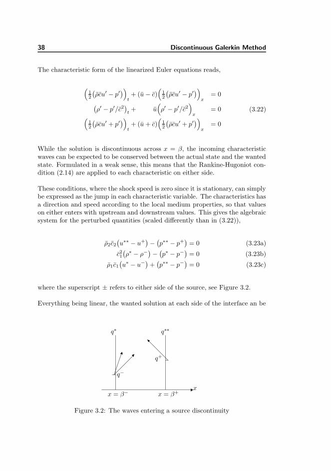
The characteristic invariants are not constant across the sources though,where also the characteristic speeds jump across the heat source, by the mediuminhomogeneity. But between the wanted state and the actual state on eitherside, we can demand the waves entering the wanted state, to be conserved, seeFigure 3.2 for a schematic representation. So on either side the conditions arewritten in terms of these propagating directions i.e. two equations from theupstream side and one from the downstream.

The weak formulation for the solution and the known hyperbolicity provides away to express the contribution to the wanted states, from the ingoing waves.


The characteristic form of the linearized Euler equations reads,

(12

(ρcu′ − p′

))t

+ (u− c)(

12

(ρcu′ − p′

))x

= 0

(ρ′ − p′/c2

)t

+ u(ρ′ − p′/c2

)x

= 0(

12

(ρcu′ + p′

))t

+ (u+ c)(

12

(ρcu′ + p′

))x

= 0

(3.22)

While the solution is discontinuous across x = β, the incoming characteristicwaves can be expected to be conserved between the actual state and the wantedstate. Formulated in a weak sense, this means that the Rankine-Hugoniot con-dition (2.14) are applied to each characteristic on either side.

These conditions, where the shock speed is zero since it is stationary, can simplybe expressed as the jump in each characteristic variable. The characteristics hasa direction and speed according to the local medium properties, so that valueson either enters with upstream and downstream values. This gives the algebraicsystem for the perturbed quantities (scaled differently than in (3.22)),

ρ2c2(u∗∗ − u+

)−(p∗∗ − p+

)= 0 (3.23a)

c21(ρ∗ − ρ−

)−(p∗ − p−

)= 0 (3.23b)

ρ1c1(u∗ − u−

)+(p∗∗ − p−

)= 0 (3.23c)

where the superscript ± refers to either side of the source, see Figure 3.2.

Everything being linear, the wanted solution at each side of the interface an be

q−

q+

q∗ q∗∗

x = β−x

x = β+

Figure 3.2: The waves entering a source discontinuity

3.3 Inclusion of sources 39

expressed, with α = γγ−1 , as a linear equation system Ax = b, with

A =

− 12 u

31

12 u

32 −

(32 ρ1u

21 + αp1

) (32 ρ2u

22 + αp2

)−αu1 αu2

−u21 u2

2 −2ρ1u1 2ρ2u2 −1 1−u1 u2 −ρ1 ρ2 0 0c21 0 0 0 −1 00 0 ρ1c2 0 1 00 0 0 ρ2c2 0 −1

(3.24a)

b =

q′

00

c21ρ− − p−

ρ1c1u− + p−

ρ2c2u+ − p+

(3.24b)

with the solution vector arranged as

x =[ρ∗ ρ∗∗ u∗ u∗∗ p∗ p∗∗

]T. (3.24c)

This system is ill-conditioned with respect to inversion because of the largeelement scale disparity. In order to avoid this ill-conditioning, the equations arerewritten in terms of nondimensional quantities. The scalings used for this arethose presented in the section 2.3 i.e. the inlet values, and this results in thefollowing system

A =

− 12M

31

12

(u2

c1

)3

−(

32M

21 + α p1

ρ1c21

) (32ρ2

ρ1

(u2

c1

)2

+ α p2

ρ1 c21

)−αM1 α u2

c1

−M21

(u2

c1

)2

−2M1 2 ρ2u2

ρ1 c1−1 1

−M1u2

c1−1 ρ2

ρ10 0

1 0 0 0 −1 00 0 c2

c10 1 0

0 0 0 ρ2 c2ρ1 c1

0 −1

(3.25a)

b =

q′/ρ1c31

00

ρ− − p−u− + p−

ρ2c2ρ1c1

u+ − p+

(3.25b)

with the tildes denoting nondimensional values. The wanted solution is thenfound in nondimensional scaling, and at each step, scaled back and fourth. This


scaling reduces the condition number significantly, from O(106) for M1 = 0.1 toO(1).

The Matlab built-in direct solver (the backslash operator) is used to solve thislinear system, which has to be done at each Runge-Kutta stage. An efficiencyimprovement would involve the factorization of the coefficient matrix A.For the inclusion of driver, a linear system is set up in the same way, althoughthe mean flow values do not differ across the source and the right hand sidevector has the source term differently. This system is also nondimensionalized.

When the unknowns are solved for, they are used to impose a state solution.This is done the same ways as with boundary conditions, such that the exterior,neighbor solution to the left of the flame is set as q+

β− = q∗ and equivalently forthe right side, where q denotes either of the three variables.

When a source is zero, the setup system is supposed to give continuous wantedstate (no source, no discontinuity). While this is the case for application ofthe driver system, the heat release calculation does not give continuous wantedstates when q′ = 0. The difference in mean flow states on either side gives, thatif the system (3.24) is used for no unsteady heat release, the wanted states arediscontinuous. On the other hand, one can argue that if no source is present,why calculate wanted states at all? So in experiments with no unsteady heatrelease, the numerical flux is applied is its usual fashion.

For the reduced isentropic system (2.15b), only the acoustic waves are present.So the conditions describing their conservation – (3.23a) and (3.23c) – are used,along with the two equations describing the heat input (2.54). These four equa-tions are set up exactly like above.

Validation of basic numerical model

Here the credibility of the scheme is sought validated. The word credibility isused on purpose, since with the used sources and an inhomogeneous medium, acorrect spatial convergence test is hard to set up. I should mention that a test onthe code for the stagnant medium for spatial convergence has been performed,the setup was a homogeneous medium without any sources, with an acousticclosed end at the left boundary and open at the right. The system was startedwith a quarter of the fundamental mode and spatial convergence was verified.This test is not included here, primarily the case of a stagnant medium is notreally used, except for calculating a reference mode frequency for the frequencydrift when a mean flow is included.The code for the moving medium was sought verified by much the same ap-

3.4 Post processing 41

proach. In a homogeneous medium without sources, the codes was run with aninitial values as the fundamental mode, e.g. for the pressure

p′(x, t = 0) = Re(A exp(−ık+x) +A exp(ık−x)

)exp(ıωt)

(3.26)

where the Doppler shifted wavenumbers are known k± = k/1 ±M . And thenumerical and the analytic solution followed each other during many periods.But the measured maximum error was not as expected, since it was dominatedby the error when the analytic solution has its rapid phase change. So I did notincluded it here.

The overall implementation is still sought validated, in the sense that it givesthe correct mode frequency with respect to the analytic frequency when thesimulation is post processed. The reference solution used later also has nounsteady heat release as an case. The method has been applied to the sametemperature distributions considered with a heat release fluctuation, and theseresults are presented in the next section.

3.4 Post processing

During the time-simulation, the primitive variables are recorded at each time-step in different positions. These time-series constitutes the data for the fre-quency analysis. The positions of these series are placed approximately halfwaysbetween left boundary and the heat source, halfways between the latter and thedriving source, and the last between the driver and the right boundary. Allin all 3 times the number of variables. In order to reduce eventual variationbetween readings at different posistions, the chosen driver is the simpel jumpcondition for velocity perturbation (2.41), so that minimal entropy fluctuationsare generated

At the end of the process, what is wanted is a frequency spectrum, representativefor the acoustics in the combustor. In order to do comparison with the analyticalsolutions, and preferably this being automatized, this spectrum should revealthe main resonance modes present in the overall domain.

So the information from all the time series are sought collected somehow. Theseseries are Hanning windowed before the FFT, not as much to render the signalperiodic, but to reduce leakage.Then a overview of ”resonance-behavior” for each spectrum is sought. This isdone by searching each spectrum for local maxima, and a sort of hit score iscollected, as the number of coinciding maxima.If a frequency has a local maximum in ≥ 2m+ 1 where m is number of system


variables, then it is treated as found in all spectra and this particular frequencystored. The number of system variables are either 2 or 3. For hits in the interval2m+1 > x ≥ m, adjacent hits (local maxima) are taken along and a mean valueis used as the found resonance frequency. And finally, in the interval m > x ≥ 1the same action is performed, except that hits in the surrounding four frequencybins are searched for hits and used to form a mean.

This process will give some uncertainty in the comparison between the numeri-cally and the analytically found resonance frequency, whenever a mean frequencyis found. Besides, the numerical found spectras have a certain frequency dis-cretization, dependent on the timestep. So finding the exact frequency downto some decimals is unrealistic. But in general, when the spectra are not to”incoherent”, a good estimate of the resonance frequency is found.

Chapter 4

Results

4.1 The Reference Solution

The results from the simulation is analysed in the frequency domain and theresonance frequencies are compared to the ”analytic” found resonance frequen-cies. These latter are found through a derivation, presented in [1], where thesound fields on either side of the flame are set up, isentropic on the upstreamside while the downstream sides carries an entropy wave in the density andtemperature fluctuations. Along with boundary conditions and the coupling ofthe fields across the heat source through the RH conditions (2.36), this can becombined into a linear system for the amplitudes of the different waves. Forwhich non-trivial solutions only exists if the determinant is zero.So this determinant expression (or characteristic polynomial), which has com-plex entries, is used to find a root in the form of a frequency, so that the systemhas a solution.

The roots are found by Newton’s method, which requires a good startingpoint in order to converge. This is less optimal in the sense of automation, sinceit is hard to know in advance what the resonance frequency are. So the startvalues are given by user by inspection of this complex function when an analyticfrequency is sought. The script doing this is not included in the Matlab codesappendix. The characteristic polynomial was found with Mathematica and isquite large, the derivative even worse.

44 Results

For the stagnant medium, the possible thermoacoustic oscillations reduced tothe roots of tan(ωβ/c1) tan(ω(L−β)/c2) = ρ1c1/ρ2c2 for the case of no unsteadyheat, and tan(ωβ/c1) tan(ω(L − β)/c2) = c1/c2 for the type of unsteady heatrelease, which the author calls ’no unsteady heat input per unit mass’ q′ =cP(T2− T1

)ρ1u′1. The suffices again refers the upstream and downstream values.

The same kind of heat sources is used when a mean flow exists i.e. no unsteadyheat (at all) and no unsteady heat input per unit mass

q′ =(cP(T2 − T1

)+ 1

2

(u2

2 − u21

))(ρ′1u1 + ρ1u

′1

). (4.1)

4.2 Results

The boundary conditions used in this reference solution is that the outlet is anopen end, while the inlet is choked and isentropic, i.e. the condition (2.24) ands′ = 0. The derivation of this solution includes this assumption of isentropicsound field upstream of the flame, so this must be fulfilled in the numericalsimulation in order to do comparison.

The hyperbolicity of the system tells us that two boundary conditions areneeded at the inflow boundary, so the zero fluctuation mass flux and isentropicityare imposed by setting the velocity and pressure fluctuations as

u′(xIN, t) = − u(xIN)

ρ(xIN)ρ′(xIN, t) and p′(xIN, t) = c2(xIN)ρ′(xIN, t) (4.2)

These imposed states will ensure that no entropy fluctuations are present up-stream of the heat release.In principle, other combinations of used variables could be used to ensure theconditions e.g. ρ′ and p′. But then the zero fluctuating mass-flux would give themean flow in the denominator, and make it less usable for low Mach numbers.This was tried, and it required the time-step to be extremely small in order tohave stability at the boundary, and therefore considered useless.

The reduced system (2.15b) only requires one boundary condition at theinlet. Isentropicity is implicitly satisfied, thus the zero fluctuation mass-fluxcondition is imposed as

u′Isentropic(xIN, t) = − u(xIN)

ρ(xIN)c2(xIN)p′(xIN, t) = − u(xIN)

γp(xIN)p′(xIN, t) (4.3)

while at the outlet, the same, single condition (pressure release) is used.

So the different tests from section 2.4 are set up with these boundary conditions,and a default geometry. The domain length was take to be a quarter of a

4.2 Results 45

wavelength, the wavelength being determined by the inlet sound speed andthe choice of 20 Hz. Inlet temperature is set to around zero degrees Celsius,or T1 = 273 K. The inlet pressure is set to 105 Pa, by which the density isfound. The mean velocity scales with the inlet Mach number, which is one ofthe tunable parameters. When simulating with a mean flow, this is taken inthe interval 1.5 · 10−4 ≤M1 ≤ 0.15. And the other parameter, the downstreamtemperature is taken in the interval T1 + 50 K ≤ T2 ≤ T1 + 550 K.

The discretization used in the experiments is 16 elements of 4’th order approx-imation, which is more than enough to resolve the waves in the system. Whenall the simulations were run, this was chosen to absolutely guarantee a sufficientresolution. When used as a simulation to get an estimate of the thermoacousticmodes, a lower discretization is sufficient, of course considering the frequencyrange.

The chamber is driven by the sweep signal in the range 10-110 Hz, and after asignal-period (1s), the recorded time-series are Fourier transformed to get thepower spectra. The resonance frequencies are then identified and compared.The reference solution does, to the best of my knowledge, not assume a con-stant mean pressure. The equations are solely described by mean velocities anddensities, sound speeds and temperatures. Of course, the mean pressure has animplicitness, but if the mean flow values are consistent, this should not do anydifference.

While for the reduced system, hopefully there is no difference. The unsteadyheat release effect is included through the reduced RH conditions (2.54), whichshould describe the influence just as well for this reduced system. As long asthe entropy wave does not interact with boundary conditions and such, the twocases should be equal.

The data are presented as the shift in frequency with respect to that particularfrequency in the stagnant medium. This is to show the mean flow effects, andscale down the results. In a figure, the x-axis is the inlet Mach number, whilethe y-axis is divided into bands. Each band represent a temperature differenceacross the heat input, where the middle of these bands is the reference no flowfrequency (a dotted line), and the full lines surrounding this is a deviation of ±5Hz. The lines with square markers is the deviation of exact frequency, while the’x’ markers denotes the numerically found resonances. If no frequency is foundfrom the simulations near that particular frequency, this case of

(M,∆T

)is left

out.

The presented figures are unfortunately not very precise in terms of exact devia-tion, but it is possible to distinguish between deviations of 2 and 4 Hz. Besides,the exact numbers are less useful, it is tendencies that are interesting.

46 Results

Starting with the comparison between the two cases of mean pressure dis-tribution in Figure 4.1 which is without the unsteady heat source . It can befaintly seen that there is a small deviation in drift frequency, also in the an-alytic frequency, but it is for larger Machs and temperature jumps only. It isnot much, but if the frequency range was broadened, it would probably be morevisible.In addition to that, the numerical method simulates the oscillations rather well,there is no sign as such of bad wave propagation. It should be mentioned thatthe third resonance frequency ∼ 160 Hz, lies outside the frequency range of theexcitation signal, but is nevertheless well excited.

Then is looked at the reduced system. In Figure 4.3 and Figure 4.4 is com-pared the reduced system with the full, without and with unsteady heat releaserespectively and both with a constant mean pressure distribution. From theseit is clear that the reduced system in this particular setup does equally well.There is a small deviation from the exact frequency in the first resonance modewhen the heat source is present, but this applies to both the reduced and the fullsystem. So it could be justified to settle with the computationally less expensivereduced system.

Finally, inspecting Figure 4.2, Figure 4.5 and Figure 4.6 reveals a surprise. Thatthe drop in mean pressure has an negative effect when the heat source is present,whether it be the full or the reduced system. The reduced system is affectedin higher frequencies even without having the heat source included. Figure 4.2which shows the full system with heat source and constant versus changingpressure reveals quite large deviation, in all the resonances considered and evenfor the smallest temperature change. And even more strange is that this effectdoes not get smaller for M → 0, where the mean flow distributions coincides.

I don’t think it is question of a flaw in the numerical model, there is no signs ofodd computations as such, all matrices to be inverted are very well conditionedand no spurious oscillations or something like that has been noticed. And thatit shows an influence on the reduced system without heat release, where nocomputations as such are performed over the material interface, is even moremystifying.It could be the data collecting, if the spectra had resonances distributed overa small interval, and hence find mean values not really representative. But thesearching of the spectra has been ”monitored”, i.e. the found frequencies wasindicated in the spectra and inspected, and no deviation was found that couldexplain this. Or else it is the expression that is used to calculate the pressurechange which is unphysical, but this also seems unreasonable. An issue forfurther study, must be the conclusion for now.

Finally a short example of the mentioned acoustic instability is presented. This

4.2 Results 47

is generate simply by changing the inlet boundary conditions, so that these arefixed mass flux along with pressure release. The outlet is still open. These inletconditions does not ensure isentropicity in the upstream field, and an entropywave is present. This affects the unsteady heat release, since this is dependenton the density fluctuation. The resulting spectrum only contains this unstablemode which can be seen in Figure 4.2 along the spectrum resulting from requir-ing isentropic boundary conditions. The inlet Mach number is set to 0.05 and∆T = 200. The spectra are normalized, so it is not evident that it really is aninstability, but after 0.3s the pressure levels were > 104. The stable spectrumalso shows the different signals, while the unstable only has this all-dominatingpeak.

48 Results

0 0.05 0.1 0.15

50

150

250

350

450

550

∆T

M

(a) 1. resonance frequency

0 0.05 0.1 0.15

50

150

250

350

450

550

∆T

M

(b) 1. resonance frequency

0 0.05 0.1 0.15

50

150

250

350

450

550

∆T

M

(c) 2. resonance frequency

0 0.05 0.1 0.15

50

150

250

350

450

550

∆T

M

(d) 2. resonance frequency

0 0.05 0.1 0.15

50

150

250

350

450

550

∆T

M

(e) 3. resonance frequency

0 0.05 0.1 0.15

50

150

250

350

450

550

∆T

M

(f) 3. resonance frequency

Figure 4.1: Full system, no unsteady heat, constant pressure in left column,pressure drop in right

4.2 Results 49

0 0.05 0.1 0.15

50

150

250

350

450

550

∆T

M


0 0.05 0.1 0.15

50

150

250

350

450

550

∆T

M


0 0.05 0.1 0.15

50

150

250

350

450

550

∆T

M


0 0.05 0.1 0.15

50

150

250

350

450

550

∆T

M


0 0.05 0.1 0.15

50

150

250

350

450

550

∆T

M


0 0.05 0.1 0.15

50

150

250

350

450

550

∆T

M


Figure 4.2: Full system, Unsteady heat, constant pressure in left column, pres-sure drop in right

50 Results

0 0.05 0.1 0.15

50

150

250

350

450

550

∆T

M


0 0.05 0.1 0.15

50

150

250

350

450

550

∆T

M


0 0.05 0.1 0.15

50

150

250

350

450

550

∆T

M


0 0.05 0.1 0.15

50

150

250

350

450

550

∆T

M


0 0.05 0.1 0.15

50

150

250

350

450

550

∆T

M


0 0.05 0.1 0.15

50

150

250

350

450

550

∆T

M


Figure 4.3: Reduced system in left, Full in right, No unsteady heat, constantpressure

4.2 Results 51

0 0.05 0.1 0.15

50

150

250

350

450

550

∆T

M


0 0.05 0.1 0.15

50

150

250

350

450

550

∆T

M


0 0.05 0.1 0.15

50

150

250

350

450

550

∆T

M


0 0.05 0.1 0.15

50

150

250

350

450

550

∆T

M


0 0.05 0.1 0.15

50

150

250

350

450

550

∆T

M


0 0.05 0.1 0.15

50

150

250

350

450

550

∆T

M


Figure 4.4: Reduced system in left, Full in right, Unsteady heat, constant pres-sure

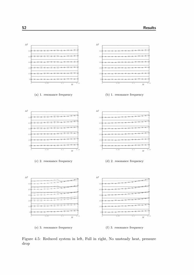
52 Results

0 0.05 0.1 0.15

50

150

250

350

450

550

∆T

M


0 0.05 0.1 0.15

50

150

250

350

450

550

∆T

M


0 0.05 0.1 0.15

50

150

250

350

450

550

∆T

M


0 0.05 0.1 0.15

50

150

250

350

450

550

∆T

M


0 0.05 0.1 0.15

50

150

250

350

450

550

∆T

M


0 0.05 0.1 0.15

50

150

250

350

450

550

∆T

M


Figure 4.5: Reduced system in left, Full in right, No unsteady heat, pressuredrop

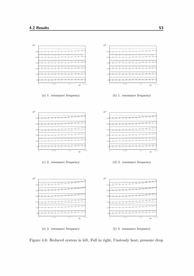
4.2 Results 53

0 0.05 0.1 0.15

50

150

250

350

450

550

∆T

M


0 0.05 0.1 0.15

50

150

250

350

450

550

∆T

M


0 0.05 0.1 0.15

50

150

250

350

450

550

∆T

M


0 0.05 0.1 0.15

50

150

250

350

450

550

∆T

M


0 0.05 0.1 0.15

50

150

250

350

450

550

∆T

M


0 0.05 0.1 0.15

50

150

250

350

450

550

∆T

M


Figure 4.6: Reduced system in left, Full in right, Unsteady heat, pressure drop

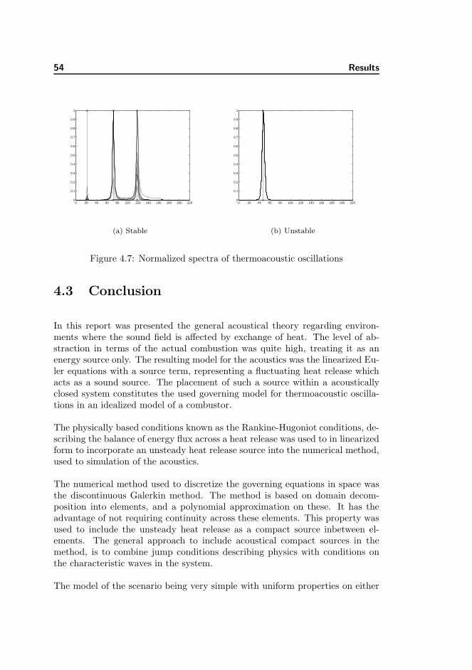
54 Results

0 20 40 60 80 100 120 140 160 180 200 2200

0.1

0.2

0.3

0.4

0.5

0.6

0.7

0.8

0.9

1

(a) Stable

0 20 40 60 80 100 120 140 160 180 200 2200

0.1

0.2

0.3

0.4

0.5

0.6

0.7

0.8

0.9

1

(b) Unstable

Figure 4.7: Normalized spectra of thermoacoustic oscillations

4.3 Conclusion

In this report was presented the general acoustical theory regarding environ-ments where the sound field is affected by exchange of heat. The level of ab-straction in terms of the actual combustion was quite high, treating it as anenergy source only. The resulting model for the acoustics was the linearized Eu-ler equations with a source term, representing a fluctuating heat release whichacts as a sound source. The placement of such a source within a acousticallyclosed system constitutes the used governing model for thermoacoustic oscilla-tions in an idealized model of a combustor.

The physically based conditions known as the Rankine-Hugoniot conditions, de-scribing the balance of energy flux across a heat release was used to in linearizedform to incorporate an unsteady heat release source into the numerical method,used to simulation of the acoustics.

The numerical method used to discretize the governing equations in space wasthe discontinuous Galerkin method. The method is based on domain decom-position into elements, and a polynomial approximation on these. It has theadvantage of not requiring continuity across these elements. This property wasused to include the unsteady heat release as a compact source inbetween el-ements. The general approach to include acoustical compact sources in themethod, is to combine jump conditions describing physics with conditions onthe characteristic waves in the system.

The model of the scenario being very simple with uniform properties on either

4.3 Conclusion 55

side of the heat source, was used to validate that the numerical model is capableof representing such a resonator model and the possible modes. A sound fieldwas generate through included driver sources, and the acoustic fluctuations wasrecorded in order to do frequency analysis. Comparison with analyticly foundresonance frequencies showed that within the overall method, including datacollecting, the method was able to capture the thermoacoustic modes within afew hertz.The advantage of using numerical simulations in the time-domain relies on thepossible excitation of many modes simultaneously.

The implementation of the analysis method in this project is a start, but far fromsufficient to be used a diagnostic tool. Although some different boundary con-ditions used frequently in the modelling of such system is included, it does notdeal with more realistic scenarios. Also the searching algorithm for resonances inthe time-series could be improved or done otherwise. But the numerical schemeitself with the source inclusion, has shown to an effective method, and since itis quite flexible, it can surely be applied to more complicated thermoacousticproblems.

56 Results

Bibliography

[1] A.P. Dowling. The calculations of thermoacoustic oscillations. Journal ofSound and Vibration, 180(4):557–581, 1995.

[2] Jan S. Hesthaven and Tim Warburton. Nodal Discontinous Galerkin Meth-ods: Algorithms, Analysis and Applications. Springer, To Appear.

[3] S.W. Rienstra and A. Hirschberg. An Introduction to Acoustics.http://www.win.tue.nl/~sjoerdr/papers/boek.pdf, 15th April 2005.

[4] O.M. Umurhan. Exploration of fundamental matters of acoustic instabilitiesin combustion chambers. Center for Turbulence Research, Stanford, AnnualResearch Briefs, 1999. http://ctr.stanford.edu/ARB99.html.

http://www.win.tue.nl/~sjoerdr/papers/boek.pdf

http://ctr.stanford.edu/ARB99.html

simulation of thermoacoustics with discontinuous …€¦ · simulation of thermoacoustics with...

Documents